An adaptive approach to real-time estimation of vehicle sideslip, road bank angles and sensor bias

Yi-Wen Liao and Francesco Borrelli Yi-Wen Liao and Francesco Borrelli are with the Department of Mechanical Engineering, University of California, Berkeley, 94720, USA. e-mail: ywliao@berkeley.edu, fborrelli@berkeley.edu.
Abstract

Robust estimation of vehicle sideslip angle is essential for stability control applications. However, the direct measurement of sideslip angle is expensive for production vehicles. This paper presents a novel sideslip estimation algorithm which relies only on sensors available on passenger and commercial vehicles. The proposed method uses both kinematics and dynamics vehicle models to construct extended Kalman filter observers. The estimate relies on the results provided from the dynamics model observer where the tire cornering stiffness parameters are updated using the information provided from the kinematics model observer. The stability property of the proposed algorithm is discussed and proven. Finally, multiple experimental tests are conducted to verify its performance in practice. The results show that the proposed approach provides smooth and accurate sideslip angle estimation. In addition, our novel algorithm provides reliable estimates of bank angles and lateral acceleration sensor bias.

Index Terms:
sideslip angle estimation, bank angle estimation, extended Kalman filter, recursive robust least square

I Introduction

Anumber of active safety features have been introduced in the automotive industry in the past 30 years to prevent accidents such as braking assistance, traction and electronic stability control systems [1, 2, 3, 4]. The main goals of these systems are to maintain vehicle stability and to improve vehicle handling. To implement these functions, vehicle states, parameters and road conditions need to be measured or estimated. Among all of these, sideslip angle, the angle between the longitudinal direction of the vehicle and the velocity vector, is one of the most important variables which heavily influences vehicle dynamics and is required by a number of active safety controllers. Although it can be directly measured by sensors such as optical sensors [5] or GPS sensors [6, 7], these solutions are not implemented by OEMs because of cost and reliability. Therefore, the estimation of sideslip angle based on the sensors available in production vehicles is an important topic that has been widely discussed in the literature [8, 9, 10, 11, 12, 13, 14, 15, 16, 17, 18, 19, 20, 21, 22, 23, 24]. Most of the approaches in the literature are model-based and can be classified into three main categories: kinematics model-based, dynamics model-based and a combination of the two.

The kinematics model-based approach proposed in [8, 9] constructs an observer based on the longitudinal and lateral translation kinematics of a point mass model. This method has the advantage of not requiring the vehicle parameters, tire model and road friction coefficient. It can provide an accurate sideslip estimate in a number of cases. However, it suffers from a drifting issue in small yaw rate maneuvers and the estimated result is sensitive to disturbance and measurement noise such as bank angles or sensor bias when the longitudinal and lateral accelerations are small. The dynamics model-based approach constructs an advanced state observer (i.e. an extended Kalman filter or an unscented Kalman filter) by using a bicycle model or its variations [10, 11, 12, 13, 14, 15, 16]. These models consider the effect of forces applied to vehicle mass and rotation inertia which provides a relatively robust estimate to acceleration measurement noise compared to the one from the kinematics model. However, an estimation bias is often observed due to the model uncertainties associated to variations of vehicle mass and the tire cornering stiffnesses. Existing literature has also focused on developing algorithms for estimating the sideslip angle and vehicle model system parameters simultaneously. In [14, 15, 16, 17], Lyapunov-based observers have been proposed for the tire cornering stiffness identification. Although these techniques can improve the estimation results, they require persistent input excitations and the adaptation performance becomes worse beyond the linear tire model region. Alternative studies have proposed learning-based techniques to assist the traditional adaptation methods [18, 19, 20]. However, the estimated performance is hard to validate in the region when data is limited. The third category of algorithms tries to merge kinematics and dynamics models into a hybrid solution [21, 22, 23, 24]. The concept is to switch between these two estimators and to exploit their respective advantages. This method might look attractive, however the switching will cause a discontinuity in the sideslip estimation. Motivated by the idea of the hybrid solution [21, 22, 23, 24] and parameter adaptation, in this paper, we develop a novel sideslip estimation algorithm which only relies on the dynamics model for the estimation but utilizes the strength of the kinematics observer to adapt the front and rear tire cornering stiffnesses. In this way, we maintain the advantage of the dynamics model-based observer and further improve the estimator performance in the nonlinear tire region. In addition, the proposed approach does not need rich input excitation as required in traditional adaptation methods.

The paper is organized as follows. We first introduce commonly used models for kinematics and dynamics-based observer designs. Then, modifications with bank angle and sensor bias effects are considered and included into each of the models. A recursive adaptation algorithm is derived and the stability property is discussed afterwards. Finally, the performance is validated with different scenario tests and compared with existing methods.
Refer to caption
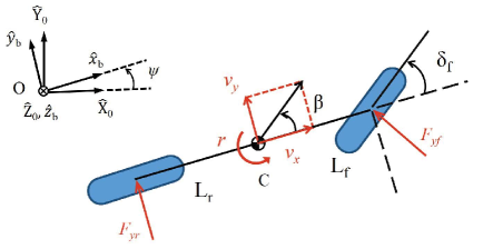
Figure 1: Lateral dynamics for bicycle model.

II Models for estimation design

Many of the conventional sideslip angle estimation methods are model-based. In this section, we are going to introduce two different models which have been frequently used in the literature [19]: a 2-DOF point mass rigid body kinematics model and a bicycle dynamics model. Each of them has its own strengths and weaknesses in the observer design. Details are discussed in the following sections.

II-A Kinematics model

Kinematics is the study of motion which treats the movement of components without considering the forces. To describe the general motion of a rigid body, we first introduce two coordinate systems followed by the ISO convention: one is fixed in the inertial space {X^0,Y^0.Z^0}formulae-sequencesubscript^𝑋0subscript^𝑌0subscript^𝑍0\{\hat{X}_{0},\hat{Y}_{0}.\hat{Z}_{0}\} and the other one is fixed to the body {x^b,y^b,z^b}subscript^𝑥𝑏subscript^𝑦𝑏subscript^𝑧𝑏\{\hat{x}_{b},\hat{y}_{b},\hat{z}_{b}\} (see Fig. 1). Then, considering the vehicle as a single rigid body constrained to move in the X^0Y^0subscript^𝑋0subscript^𝑌0\hat{X}_{0}\hat{Y}_{0}-plane, the translation motion is described as:

ax=v˙xrvyay=v˙y+rvxsubscript𝑎𝑥subscript˙𝑣𝑥𝑟subscript𝑣𝑦subscript𝑎𝑦subscript˙𝑣𝑦𝑟subscript𝑣𝑥\displaystyle\begin{split}a_{x}=\dot{v}_{x}-rv_{y}\\ a_{y}=\dot{v}_{y}+rv_{x}\end{split} (1)

where ψ𝜓\psi is the yaw angle, r=Δψ˙𝑟Δ˙𝜓r\overset{\Delta}{=}\dot{\psi} is the yaw rate of the vehicle. axsubscript𝑎𝑥a_{x} and vxsubscript𝑣𝑥v_{x} denote the inertial acceleration and velocity resolved in the longitudinal x^bsubscript^𝑥𝑏\hat{x}_{b}-direction. aysubscript𝑎𝑦a_{y} and vysubscript𝑣𝑦v_{y} denote the same physical quantities but resolved in the lateral y^bsubscript^𝑦𝑏\hat{y}_{b}-direction. Define the sideslip angle as

β=tan1(vy/vx).𝛽superscript1subscript𝑣𝑦subscript𝑣𝑥\displaystyle\beta=\tan^{-1}(v_{y}/v_{x}).

We write the system (1) into a standard state space form as:

𝐱˙k=Ak(t)𝐱k+Bk(t)𝐮k𝐲k=Ck(t)𝐱ksubscript˙𝐱𝑘subscript𝐴𝑘𝑡subscript𝐱𝑘subscript𝐵𝑘𝑡subscript𝐮𝑘subscript𝐲𝑘subscript𝐶𝑘𝑡subscript𝐱𝑘\displaystyle\begin{split}\dot{\mathbf{x}}_{k}&=A_{k}(t)\mathbf{x}_{k}+B_{k}(t)\mathbf{u}_{k}\\ \mathbf{y}_{k}&=C_{k}(t)\mathbf{x}_{k}\end{split} (2)

where 𝐱k=[vx,vy]Tsubscript𝐱𝑘superscriptdelimited-[]subscript𝑣𝑥,subscript𝑣𝑦𝑇\mathbf{x}_{k}=[v_{x}\text{,}~{}v_{y}]^{T} is the state vector, 𝐮k=[ax,ay]Tsubscript𝐮𝑘superscriptsubscript𝑎𝑥subscript𝑎𝑦𝑇\mathbf{u}_{k}=[a_{x},~{}a_{y}]^{T} is the control input vector, 𝐲k=vxsubscript𝐲𝑘subscript𝑣𝑥\mathbf{y}_{k}=v_{x} is the measurement output vector and the system, input and output matrices are

Ak(t)=[0r(t)r(t)0],Bk(t)=[1001]Ck(t)=[10].formulae-sequencesubscript𝐴𝑘𝑡matrix0𝑟𝑡𝑟𝑡0subscript𝐵𝑘𝑡matrix1001subscript𝐶𝑘𝑡matrix10\displaystyle\begin{split}A_{k}(t)&=\begin{bmatrix}0&~{}r(t)\\ -r(t)&~{}0\end{bmatrix},~{}~{}B_{k}(t)=\begin{bmatrix}1&0\\ 0&1\end{bmatrix}\\ C_{k}(t)&=\begin{bmatrix}1~{}~{}0\end{bmatrix}.\end{split} (3)

As explained in [25], using the kinematics model is advantageous as it allows a sideslip angle estimation without requiring vehicle parameters. All we need is r𝑟r, axsubscript𝑎𝑥a_{x}, aysubscript𝑎𝑦a_{y} and vxsubscript𝑣𝑥v_{x} which can be directly obtained from sensors available in commercial vehicles. However, the estimation is sensitive to sensor noise which is substantial for axsubscript𝑎𝑥a_{x} and aysubscript𝑎𝑦a_{y}. Moreover, the convergence of the estimation error can be guaranteed only when yaw rate is not equal to zero. In fact, the system (2) is not observable when the yaw rate is equal to zero and the poor conditioning of the observability matrix causes a drifting problem. This can be avoided by resetting the estimated states to zero every time when yaw rate is less than a threshold value.

II-B Dynamics model

A variety of dynamics models have appeared in the literature. The so-called lateral bicycle model shown in Fig. 1 is a widely used and rather simple model that neglects the coupling of the roll, pitch and longitudinal dynamics. By using Newton’s law of motion, the lateral dynamics of the bicycle model is described as follows [26]:

may=m(v˙y+vxr)=Fyfcosδf+FyrIzr˙=LfFyfcosδfLrFyr𝑚subscript𝑎𝑦𝑚subscript˙𝑣𝑦subscript𝑣𝑥𝑟subscript𝐹𝑦𝑓subscript𝛿𝑓subscript𝐹𝑦𝑟subscript𝐼𝑧˙𝑟subscript𝐿𝑓subscript𝐹𝑦𝑓subscript𝛿𝑓subscript𝐿𝑟subscript𝐹𝑦𝑟\displaystyle\begin{split}ma_{y}&=m(\dot{v}_{y}+v_{x}r)=F_{yf}\cos\delta_{f}+F_{yr}\\ I_{z}\dot{r}&=L_{f}F_{yf}\cos\delta_{f}-L_{r}F_{yr}\end{split} (4)

where m𝑚m is the vehicle mass, Izsubscript𝐼𝑧I_{z} is the equivalent yaw moment of inertia, δfsubscript𝛿𝑓\delta_{f} is the front steering angle and Lfsubscript𝐿𝑓L_{f}, Lrsubscript𝐿𝑟L_{r} are the distance from the vehicle center of gravity (COG) to the front and rear axles. To further simplify the model, we assume small tire slip and front steering angles. Then, the front and the rear lateral tire forces Fyfsubscript𝐹𝑦𝑓F_{yf}, Fyrsubscript𝐹𝑦𝑟F_{yr} can be approximated by a linear function:

FyfcosδfFyf=Cf(δfvy+Lfrvx)Fyr=Cr(vy+Lrrvx)subscript𝐹𝑦𝑓subscript𝛿𝑓subscript𝐹𝑦𝑓subscript𝐶𝑓subscript𝛿𝑓subscript𝑣𝑦subscript𝐿𝑓𝑟subscript𝑣𝑥subscript𝐹𝑦𝑟subscript𝐶𝑟subscript𝑣𝑦subscript𝐿𝑟𝑟subscript𝑣𝑥\displaystyle\begin{split}F_{yf}\cos\delta_{f}\approx F_{yf}&=C_{f}\left(\delta_{f}-\frac{v_{y}+L_{f}r}{v_{x}}\right)\\ F_{yr}&=C_{r}\left(\frac{-v_{y}+L_{r}r}{v_{x}}\right)\end{split} (5)

where Cfsubscript𝐶𝑓C_{f} and Crsubscript𝐶𝑟C_{r} are the front and rear tire cornering stiffnesses. Substituting (5) into (4), we then obtain a nonlinear model. Assume that the vehicle is traveling with slowly varying longitudinal velocity. At each step, a linearization process will be applied to approximate the nonlinear system (4)-(5) with a linear time varying system shown as follows:

𝐱˙d=Ad(t)𝐱d+Bd(t)𝐮d𝐲d=Cd(t)𝐱d+Dd(t)𝐮dsubscript˙𝐱𝑑subscript𝐴𝑑𝑡subscript𝐱𝑑subscript𝐵𝑑𝑡subscript𝐮𝑑subscript𝐲𝑑subscript𝐶𝑑𝑡subscript𝐱𝑑subscript𝐷𝑑𝑡subscript𝐮𝑑\displaystyle\begin{split}\dot{\mathbf{x}}_{d}&=A_{d}(t)\mathbf{x}_{d}+B_{d}(t)\mathbf{u}_{d}\\ \mathbf{y}_{d}&=C_{d}(t)\mathbf{x}_{d}+D_{d}(t)\mathbf{u}_{d}\end{split} (6)

where 𝐱d=[vy,r]Tsubscript𝐱𝑑superscriptsubscript𝑣𝑦𝑟𝑇\mathbf{x}_{d}=[v_{y},~{}r]^{T} is the state vector, 𝐮d=δfsubscript𝐮𝑑subscript𝛿𝑓\mathbf{u}_{d}=\delta_{f} is the control input vector and 𝐲d=[ay,r]Tsubscript𝐲𝑑superscriptsubscript𝑎𝑦𝑟𝑇\mathbf{y}_{d}=[a_{y},~{}r]^{T} is the measurement output vector.

Ad(t)=[CfCrmvx(t)vx(t)LfCfLrCrmvx(t)LfCf+LrCrIzvx(t)Lf2CfLr2CrIzvx(t)],Cd(t)=[CfCrmvx(t)LfCfLrCrmvx(t)01],Bd(t)=[CfmLfCfIz],Dd(t)=[Cfm0].formulae-sequencesubscript𝐴𝑑𝑡matrixsubscript𝐶𝑓subscript𝐶𝑟𝑚subscript𝑣𝑥𝑡subscript𝑣𝑥𝑡subscript𝐿𝑓subscript𝐶𝑓subscript𝐿𝑟subscript𝐶𝑟𝑚subscript𝑣𝑥𝑡subscript𝐿𝑓subscript𝐶𝑓subscript𝐿𝑟subscript𝐶𝑟subscript𝐼𝑧subscript𝑣𝑥𝑡superscriptsubscript𝐿𝑓2subscript𝐶𝑓superscriptsubscript𝐿𝑟2subscript𝐶𝑟subscript𝐼𝑧subscript𝑣𝑥𝑡formulae-sequencesubscript𝐶𝑑𝑡matrixsubscript𝐶𝑓subscript𝐶𝑟𝑚subscript𝑣𝑥𝑡subscript𝐿𝑓subscript𝐶𝑓𝐿𝑟subscript𝐶𝑟𝑚subscript𝑣𝑥𝑡01formulae-sequencesubscript𝐵𝑑𝑡matrixsubscript𝐶𝑓𝑚subscript𝐿𝑓subscript𝐶𝑓subscript𝐼𝑧subscript𝐷𝑑𝑡matrixsubscript𝐶𝑓𝑚0\displaystyle\begin{split}A_{d}(t)&=\begin{bmatrix}\frac{-C_{f}-C_{r}}{mv_{x}(t)}&-v_{x}(t)-\frac{L_{f}C_{f}-L_{r}C_{r}}{mv_{x}(t)}\\ \frac{-L_{f}C_{f}+L_{r}C_{r}}{I_{z}v_{x}(t)}&\frac{-L_{f}^{2}C_{f}-L_{r}^{2}C_{r}}{I_{z}v_{x}(t)}\end{bmatrix},\\ C_{d}(t)&=\begin{bmatrix}\frac{-C_{f}-C_{r}}{mv_{x}(t)}~{}&~{}-\frac{L_{f}C_{f}-LrC_{r}}{mv_{x}(t)}\\ 0~{}&~{}1\end{bmatrix},\\ B_{d}(t)&=\begin{bmatrix}\frac{C_{f}}{m}\\ \frac{L_{f}C_{f}}{I_{z}}\end{bmatrix},~{}~{}~{}D_{d}(t)=\begin{bmatrix}\frac{C_{f}}{m}\\ 0\end{bmatrix}.~{}~{}~{}~{}~{}\end{split} (7)

Using the dynamics bicycle model to estimate the sideslip angle has several advantages. First, the estimator can be tuned to be less sensitive to acceleration measurement noise compared to the one based on the kinematics model. Also, drifting and observability issues of the kinematics model are not present. However, the estimated accuracy is affected by the vehicle parameters in the matrices (7). First, since we use a linear tire model, the sideslip estimate will be accurate only in the linear tire region. Second, compared to m𝑚m, Izsubscript𝐼𝑧I_{z}, Lfsubscript𝐿𝑓L_{f} and Lrsubscript𝐿𝑟L_{r}, it is hard to find a good initial condition for the tire cornering stiffness coefficients. To mitigate this issue, on-line adaptation algorithms have been introduced to identify the cornering stiffness [15, 16]. We will also use this idea in our method.

III New sideslip estimation method

The method proposed in this paper relates to the idea of [22] which merges the kinematics and dynamics model observers into a hybrid solution. Since the estimated state from the kinematics model is unaffected by the parameter uncertainties, in [22], the observer is built to mainly rely on it but will switch to the dynamics model when the absolute value of the yaw rate is less than a threshold value rtsubscript𝑟𝑡r_{t} to avoid unobservability and the drifting issue. Although this method addresses the drifting issue, relying on the kinematics model leads to noisy estimates. Moreover, the switch between the kinematics and dynamics models for the observer often introduces a discontinuous estimate during the transition.

To overcome these issues and keep the benefits of hybrid models, we propose a new method which is based on a dynamics model but adapts on-line the front and rear tire cornering stiffnesses using information derived from the kinematics model. Compared with the traditional adaptation algorithm proposed in [15, 16], the proposed approach does not need persistent excitation in the control input and also improves the adaptation performance in the nonlinear tire region. For the observer design, we further include the road bank angle disturbance and lateral acceleration sensor bias into the system model in order to minimize possible modeling and estimation errors. This is discussed in next.

III-A Augmented Models

III-A1 Dynamics model augmented with the road bank angle and sensor bias

We consider the bicycle model and include the gravitational force to the lateral dynamics:

m(v˙y+vxr)=Fyfcosδf+Fyrmgsinϕ𝑚subscript˙𝑣𝑦subscript𝑣𝑥𝑟subscript𝐹𝑦𝑓subscript𝛿𝑓subscript𝐹𝑦𝑟𝑚𝑔italic-ϕ\displaystyle m(\dot{v}_{y}+v_{x}r)=F_{yf}\cos\delta_{f}+F_{yr}-mg\sin\phi (8)

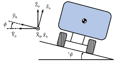
where ϕitalic-ϕ\phi is the road bank angle with the sign convention shown in Fig. 2. Then, combining the yaw dynamics in (4) with (8), we rewrite the first equation of (6) as:

v˙y=(Cf+Cr)mvxvy(vx+\displaystyle\dot{v}_{y}=\frac{-(C_{f}+C_{r})}{mv_{x}}v_{y}-(v_{x}+ LfCfLrCrmvx)r\displaystyle\frac{L_{f}C_{f}-L_{r}C_{r}}{mv_{x}})r
gsinϕ+Cfmδf.𝑔italic-ϕsubscript𝐶𝑓𝑚subscript𝛿𝑓\displaystyle~{}~{}~{}~{}~{}-g\sin\phi+\frac{C_{f}}{m}\delta_{f}. (9)

The measurement model should also be corrected with the bank disturbance and sensor bias as well. Note that the lateral accelerometer measures the right hand side of (8) divided by m𝑚m and plus the component of gravity in y^bsubscript^𝑦𝑏\hat{y}_{b} direction. We obtain the measurement model of the lateral acceleration as:

aysensuperscriptsubscript𝑎𝑦𝑠𝑒𝑛\displaystyle a_{y}^{sen} =ay+gsinϕ+d=v˙y+vxr+gsinϕ+dabsentsubscript𝑎𝑦𝑔italic-ϕ𝑑subscript˙𝑣𝑦subscript𝑣𝑥𝑟𝑔italic-ϕ𝑑\displaystyle=a_{y}+g\sin\phi+d=\dot{v}_{y}+v_{x}r+g\sin\phi+d (10)
=(Cf+Cr)mvx(t)vyLfCfLrCrmvx(t)r+d+Cfmδf.absentsubscript𝐶𝑓subscript𝐶𝑟𝑚subscript𝑣𝑥𝑡subscript𝑣𝑦subscript𝐿𝑓subscript𝐶𝑓subscript𝐿𝑟subscript𝐶𝑟𝑚subscript𝑣𝑥𝑡𝑟𝑑subscript𝐶𝑓𝑚subscript𝛿𝑓\displaystyle=\frac{-(C_{f}+C_{r})}{mv_{x}(t)}v_{y}-\frac{L_{f}C_{f}-L_{r}C_{r}}{mv_{x}(t)}r+d+\frac{C_{f}}{m}\delta_{f}.

where d𝑑d is the sensor bias. By augmenting the system with a constant bank angle disturbance and the sensor bias, the state vector and measurement output are 𝐱d=[vy,r,sinϕ,d]Tsubscript𝐱𝑑superscriptsubscript𝑣𝑦𝑟italic-ϕ𝑑𝑇\mathbf{x}_{d}=[v_{y},~{}r,~{}\sin\phi,~{}~{}d]^{T} and 𝐲d=[aysen,r]Tsubscript𝐲𝑑superscriptsuperscriptsubscript𝑎𝑦𝑠𝑒𝑛𝑟𝑇\mathbf{y}_{d}=[a_{y}^{sen},~{}r]^{T}. The system state space matrices which replace the one in (7) are

Ad(t)subscript𝐴𝑑𝑡\displaystyle A_{d}(t) =[CfCrmvx(t)vx(t)LfCfLrCrmvx(t)g0LfCf+LrCrIzvx(t)Lf2CfLr2CrIzvx(t)0000000000],absentmatrixsubscript𝐶𝑓subscript𝐶𝑟𝑚subscript𝑣𝑥𝑡subscript𝑣𝑥𝑡subscript𝐿𝑓subscript𝐶𝑓subscript𝐿𝑟subscript𝐶𝑟𝑚subscript𝑣𝑥𝑡𝑔0subscript𝐿𝑓subscript𝐶𝑓subscript𝐿𝑟subscript𝐶𝑟subscript𝐼𝑧subscript𝑣𝑥𝑡superscriptsubscript𝐿𝑓2subscript𝐶𝑓superscriptsubscript𝐿𝑟2subscript𝐶𝑟subscript𝐼𝑧subscript𝑣𝑥𝑡0000000000\displaystyle=\begin{bmatrix}\frac{-C_{f}-C_{r}}{mv_{x}(t)}&-v_{x}(t)-\frac{L_{f}C_{f}-L_{r}C_{r}}{mv_{x}(t)}&-g&0\\ \frac{-L_{f}C_{f}+L_{r}C_{r}}{I_{z}v_{x}(t)}&\frac{-L_{f}^{2}C_{f}-L_{r}^{2}C_{r}}{I_{z}v_{x}(t)}&0&0\\ 0&0&0&0\\ 0&0&0&0\end{bmatrix},
Cd(t)subscript𝐶𝑑𝑡\displaystyle C_{d}(t) =[CfCrmvx(t)LfCfLrCrmvx(t)010100],absentmatrixsubscript𝐶𝑓subscript𝐶𝑟𝑚subscript𝑣𝑥𝑡subscript𝐿𝑓subscript𝐶𝑓subscript𝐿𝑟subscript𝐶𝑟𝑚subscript𝑣𝑥𝑡010100\displaystyle=\begin{bmatrix}\frac{-C_{f}-C_{r}}{mv_{x}(t)}&-\frac{L_{f}C_{f}-L_{r}C_{r}}{mv_{x}(t)}&0&1\\ 0&1&0&0\end{bmatrix}, (11)
Bd(t)subscript𝐵𝑑𝑡\displaystyle B_{d}(t) =[CfmLfCfIz00],Dd(t)=[Cfm0].formulae-sequenceabsentmatrixsubscript𝐶𝑓𝑚subscript𝐿𝑓subscript𝐶𝑓subscript𝐼𝑧00subscript𝐷𝑑𝑡matrixsubscript𝐶𝑓𝑚0\displaystyle=\begin{bmatrix}\frac{C_{f}}{m}\\ \frac{L_{f}C_{f}}{I_{z}}\\ 0\\ 0\end{bmatrix},~{}~{}~{}~{}~{}~{}D_{d}(t)=\begin{bmatrix}\frac{C_{f}}{m}\\ 0\end{bmatrix}.~{}~{}~{}~{}~{}

To implement the extended Kalman filter using a digital controller, we further discretized model (11) using a forward Euler method as:

𝐱^d[k+1]subscript^𝐱𝑑delimited-[]𝑘1\displaystyle\hat{\mathbf{x}}_{d}[k+1] =(Ad[k]Δt+I4)𝐱^d[k]+Bd[k]Δt𝐮d[k]+𝐰d[k]absentsubscript𝐴𝑑delimited-[]𝑘Δ𝑡subscriptI4subscript^𝐱𝑑delimited-[]𝑘subscript𝐵𝑑delimited-[]𝑘Δ𝑡subscript𝐮𝑑delimited-[]𝑘subscript𝐰𝑑delimited-[]𝑘\displaystyle=(A_{d}[k]\Delta t+\text{I}_{4})\hat{\mathbf{x}}_{d}[k]+B_{d}[k]\Delta t\mathbf{u}_{d}[k]+\mathbf{w}_{d}[k]
𝐲d[k]subscript𝐲𝑑delimited-[]𝑘\displaystyle\mathbf{y}_{d}[k] =Cd[k]𝐱^d[k]+Dd[k]𝐮d[k]+𝐯d[k]absentsubscript𝐶𝑑delimited-[]𝑘subscript^𝐱𝑑delimited-[]𝑘subscript𝐷𝑑delimited-[]𝑘subscript𝐮𝑑delimited-[]𝑘subscript𝐯𝑑delimited-[]𝑘\displaystyle=C_{d}[k]\hat{\mathbf{x}}_{d}[k]+D_{d}[k]\mathbf{u}_{d}[k]+\mathbf{v}_{d}[k] (12)

where ΔtΔ𝑡\Delta t is the sampling period and [\cdot] represent the discrete time instant. 𝐰d[]subscript𝐰𝑑delimited-[]\mathbf{w}_{d}[\cdot] and 𝐯d[]subscript𝐯𝑑delimited-[]\mathbf{v}_{d}[\cdot] are the process and measurement noises satisfying the typical assumptions of the extended Kalman filter.
Refer to caption
Figure 2: Sign convention for bank angle.
Algorithm 1 Sideslip Angle Estimation
1:initialize
2:      𝐱^k[0][vx[0]vy[0]0]Tsubscript^𝐱𝑘delimited-[]0superscriptdelimited-[]subscript𝑣𝑥delimited-[]0subscript𝑣𝑦delimited-[]00𝑇\hat{\mathbf{x}}_{k}[0]\leftarrow[v_{x}[0]~{}v_{y}[0]~{}0]^{T},  𝐱^d[0][vy[0]r[0]00]Tsubscript^𝐱𝑑delimited-[]0superscriptdelimited-[]subscript𝑣𝑦delimited-[]0𝑟delimited-[]000𝑇\hat{\mathbf{x}}_{d}[0]\leftarrow[v_{y}[0]~{}r[0]~{}0~{}~{}0]^{T},   θ~00subscriptsuperscript~𝜃00\tilde{\theta}^{*}_{0}\leftarrow 0,   R00subscript𝑅00R_{0}\leftarrow 0,  θ0θ++θ~0superscriptsubscript𝜃0superscript𝜃subscriptsuperscript~𝜃0\theta_{0}^{*}\leftarrow{\theta}^{+}+\tilde{\theta}^{*}_{0},
3:    Pk[0]Pk,0subscript𝑃𝑘delimited-[]0subscript𝑃𝑘0P_{k}[0]\leftarrow P_{k,0},  Pd[0]Pd,0subscript𝑃𝑑delimited-[]0subscript𝑃𝑑0P_{d}[0]\leftarrow P_{d,0}                     // initialize prior means and estimate error covariance matrices for EKF
4:for i = 1 to k+1 do
5:     𝐱^d[i]subscript^𝐱𝑑delimited-[]𝑖absent\hat{\mathbf{x}}_{d}[i]\leftarrow EKFupdate(𝐱^d[i1],𝐮d[i1],𝐮d[i],𝐲d[i],Pd[i1],θi1subscript^𝐱𝑑delimited-[]𝑖1subscript𝐮𝑑delimited-[]𝑖1subscript𝐮𝑑delimited-[]𝑖subscript𝐲𝑑delimited-[]𝑖subscript𝑃𝑑delimited-[]𝑖1subscriptsuperscript𝜃𝑖1\hat{\mathbf{x}}_{d}[i-1],\mathbf{u}_{d}[i-1],\mathbf{u}_{d}[i],\mathbf{y}_{d}[i],P_{d}[i-1],\theta^{*}_{i-1})      // EKF update with model (12)
6:     𝐱^k[i]subscript^𝐱𝑘delimited-[]𝑖absent\hat{\mathbf{x}}_{k}[i]\leftarrow EKFupdate(𝐱^k[i1],𝐮k[i1],𝐲k[i],Pk[i1]subscript^𝐱𝑘delimited-[]𝑖1subscript𝐮𝑘delimited-[]𝑖1subscript𝐲𝑘delimited-[]𝑖subscript𝑃𝑘delimited-[]𝑖1\hat{\mathbf{x}}_{k}[i-1],\mathbf{u}_{k}[i-1],\mathbf{y}_{k}[i],P_{k}[i-1]))                  // EKF update with model (15)
7:     if |ri|rtsubscript𝑟𝑖subscript𝑟𝑡|r_{i}|\geq r_{t} then
8:         Ri=λRi1+ΦiΦiTsubscript𝑅𝑖𝜆subscript𝑅𝑖1subscriptΦ𝑖superscriptsubscriptΦ𝑖𝑇R_{i}=\lambda R_{i-1}+\Phi_{i}\Phi_{i}^{T}                           // obtain the input measurement ΦisubscriptΦ𝑖\Phi_{i} from (18)
9:         θiθ++subscriptsuperscript𝜃𝑖limit-fromsuperscript𝜃\theta^{*}_{i}\leftarrow{\theta}^{+}+ AdaptationUpdate(Ri,θ~i1subscript𝑅𝑖subscriptsuperscript~𝜃𝑖1R_{i},\tilde{\theta}^{*}_{i-1})      // apply the recursive update law (21) for the tire cornering stiffnesses
10:     else
11:         θiθi1subscriptsuperscript𝜃𝑖subscriptsuperscript𝜃𝑖1\theta^{*}_{i}\leftarrow\theta^{*}_{i-1}
12:         𝐱^k[i][vx[i]v^y,d[i]sinϕ^d[i]]Tsubscript^𝐱𝑘delimited-[]𝑖superscriptdelimited-[]subscript𝑣𝑥delimited-[]𝑖subscript^𝑣𝑦𝑑delimited-[]𝑖subscript^italic-ϕ𝑑delimited-[]𝑖𝑇\hat{\mathbf{x}}_{k}[i]\leftarrow[v_{x}[i]~{}\hat{v}_{y,d}[i]~{}\sin\hat{\phi}_{d}[i]]^{T}             // update the state estimates of the EKF for model (15)
13:         Pk[i]diag(0,Pd[i](1,1),Pd[i](3,3))subscript𝑃𝑘delimited-[]𝑖diag0subscript𝑃𝑑delimited-[]𝑖11subscript𝑃𝑑delimited-[]𝑖33P_{k}[i]\leftarrow\text{diag}(0,P_{d}[i](1,1),P_{d}[i](3,3))      // update error covariance matrix of the EKF for model (15)
14:     end if
15:     β[i]tan1(v^y,d[i]/vx[i])𝛽delimited-[]𝑖superscript1subscript^𝑣𝑦𝑑delimited-[]𝑖subscript𝑣𝑥delimited-[]𝑖\beta[i]\leftarrow\tan^{-1}(\hat{v}_{y,d}[i]/v_{x}[i])                       // calculate sideslip angle
16:end for

III-A2 Kinematics model augmented with the road bank angle

For the kinematics model, we only include the bank angle disturbance into the lateral motion by noting that the system is not observable if the model of the sensor bias is added. The model becomes:

axsubscript𝑎𝑥\displaystyle a_{x} =v˙xrvyabsentsubscript˙𝑣𝑥𝑟subscript𝑣𝑦\displaystyle=\dot{v}_{x}-rv_{y}
aysensuperscriptsubscript𝑎𝑦𝑠𝑒𝑛\displaystyle a_{y}^{sen} =v˙y+rvx+gsinϕ.absentsubscript˙𝑣𝑦𝑟subscript𝑣𝑥𝑔italic-ϕ\displaystyle=\dot{v}_{y}+rv_{x}+g\sin\phi. (13)

Then, having the same extended Kalman filter structure shown in (12), we re-define the state vector 𝐱k=[vx,vy,sinϕ]Tsubscript𝐱𝑘superscriptsubscript𝑣𝑥subscript𝑣𝑦italic-ϕ𝑇\mathbf{x}_{k}=[v_{x},~{}v_{y},~{}\sin\phi]^{T}, the output vector 𝐮k=[ax,aysen]Tsubscript𝐮𝑘superscriptsubscript𝑎𝑥superscriptsubscript𝑎𝑦𝑠𝑒𝑛𝑇\mathbf{u}_{k}=[a_{x},~{}a_{y}^{sen}]^{T} and the system state space matrices as

Ak(t)=[0r(t)0r(t)0g000],Bk(t)=[1001],Ck(t)=[100].formulae-sequencesubscript𝐴𝑘𝑡matrix0𝑟𝑡0𝑟𝑡0𝑔000formulae-sequencesubscript𝐵𝑘𝑡matrix1001subscript𝐶𝑘𝑡matrix100\displaystyle\begin{split}A_{k}(t)&=\begin{bmatrix}~{}0&r(t)&0\\ -r(t)&0&-g\\ ~{}0&0&0\end{bmatrix},~{}~{}~{}B_{k}(t)=\begin{bmatrix}~{}1&0~{}\\ ~{}0&1~{}\end{bmatrix},\\ C_{k}(t)&=\begin{bmatrix}~{}1~{}&~{}0~{}&~{}0~{}\end{bmatrix}.\end{split} (14)

The above model is, again, discretized into:

𝐱^k[k+1]subscript^𝐱𝑘delimited-[]𝑘1\displaystyle\hat{\mathbf{x}}_{k}[k+1] =(Ak[k]Δt+I3)𝐱^k[k]+Bk[k]Δt𝐮k[k]+𝐰k[k]absentsubscript𝐴𝑘delimited-[]𝑘Δ𝑡subscriptI3subscript^𝐱𝑘delimited-[]𝑘subscript𝐵𝑘delimited-[]𝑘Δ𝑡subscript𝐮𝑘delimited-[]𝑘subscript𝐰𝑘delimited-[]𝑘\displaystyle=(A_{k}[k]\Delta t+\text{I}_{3})\hat{\mathbf{x}}_{k}[k]+B_{k}[k]\Delta t\mathbf{u}_{k}[k]+\mathbf{w}_{k}[k]
𝐲k[k+1]subscript𝐲𝑘delimited-[]𝑘1\displaystyle\mathbf{y}_{k}[k+1] =Ck[k+1]𝐱^k[k+1]+𝐯k[k+1].absentsubscript𝐶𝑘delimited-[]𝑘1subscript^𝐱𝑘delimited-[]𝑘1subscript𝐯𝑘delimited-[]𝑘1\displaystyle=C_{k}[k+1]\hat{\mathbf{x}}_{k}[k+1]+\mathbf{v}_{k}[k+1]. (15)

III-B Adaptation for the tire cornering stiffness

In the previous section, we have introduced two observer models (12) and (15). Next, we will show how we merge both observers by using v^y,ksubscript^𝑣𝑦𝑘\hat{v}_{y,k}, the lateral velocity estimated from (15), to adapt the front and rear tire cornering stiffnesses in the dynamics model (12). The sideslip estimation will then calculate by using this updated dynamics model.

III-B1 Regression model

The adaptation is formulated as a regularized weighted least square (RWLS) problem [27, 28]. To build up the adaptation algorithm, we first specify the regression model as

Y=ΦTθ𝑌superscriptΦ𝑇𝜃\displaystyle Y=\Phi^{T}\theta (16)

where θ𝜃\theta is the parameter to be estimated; ΦΦ\Phi and Y𝑌Y are the input and output measurements. Substituting equation (13) into (9), the aysubscript𝑎𝑦a_{y} measurement can be expressed as follows:

aysensuperscriptsubscript𝑎𝑦𝑠𝑒𝑛\displaystyle a_{y}^{sen} =v˙y+vxr+gsinϕabsentsubscript˙𝑣𝑦subscript𝑣𝑥𝑟𝑔italic-ϕ\displaystyle=\dot{v}_{y}+v_{x}r+g\sin\phi
=(Cf+Cr)mvxvyLfCfLrCrmvxr+Cfmδf.absentsubscript𝐶𝑓subscript𝐶𝑟𝑚subscript𝑣𝑥subscript𝑣𝑦subscript𝐿𝑓subscript𝐶𝑓subscript𝐿𝑟subscript𝐶𝑟𝑚subscript𝑣𝑥𝑟subscript𝐶𝑓𝑚subscript𝛿𝑓\displaystyle=\frac{-(C_{f}+C_{r})}{mv_{x}}v_{y}-\frac{L_{f}C_{f}-L_{r}C_{r}}{mv_{x}}r+\frac{C_{f}}{m}\delta_{f}. (17)

Then, combining (17) with the yaw rate dynamics, we define the regression model as:

ΦT=[Lf2rLfv^y,kvx+LfδfLr2r+Lrv^y,kvxLfrv^y,kvx+δfLrrv^y,kvx],Y=[Izr˙maysen],θ=[CfCr]\displaystyle\begin{split}\Phi^{T}&=\begin{bmatrix}\frac{-L_{f}^{2}r-L_{f}\hat{v}_{y,k}}{v_{x}}+L_{f}\delta_{f}&~{}\frac{-L_{r}^{2}r+L_{r}\hat{v}_{y,k}}{v_{x}}\\ \frac{-L_{f}r-\hat{v}_{y,k}}{v_{x}}+\delta_{f}&~{}\frac{L_{r}r-\hat{v}_{y,k}}{v_{x}}\end{bmatrix},\\ Y&=\begin{bmatrix}I_{z}\dot{r}\\ ma_{y}^{\text{sen}}\end{bmatrix},~{}~{}~{}~{}~{}\theta=\begin{bmatrix}C_{f}\\ C_{r}\end{bmatrix}\end{split} (18)

where the unknown lateral velocity is replaced by v^y,ksubscript^𝑣𝑦𝑘\hat{v}_{y,k} estimated from the kinematics model. Observe that all the other time-varying variables in the input and output measurements can be directly obtained from the standard sensors for yaw stability control system. The angular acceleration is obtained by differentiating the yaw rate: (r[k]r[k1])/Δt𝑟delimited-[]𝑘𝑟delimited-[]𝑘1Δ𝑡(r[k]-r[k-1])/\Delta t with a low-pass filter.

III-B2 Adaptation algorithm

Considering all the input and output data sampled at time instant iΔt𝑖Δ𝑡i\Delta t, where i=1,2,k𝑖12𝑘i=1,2,...k is the time step, we want to minimize the sum of the squared prediction errors:

J(θk)=i=1kλ(ki)YiΦiTθk22+δθkθ+22𝐽subscript𝜃𝑘superscriptsubscript𝑖1𝑘superscript𝜆𝑘𝑖superscriptsubscriptnormsubscript𝑌𝑖superscriptsubscriptΦ𝑖𝑇subscript𝜃𝑘22𝛿superscriptsubscriptnormsubscript𝜃𝑘superscript𝜃22\displaystyle J(\theta_{k})=\sum_{i=1}^{k}\lambda^{(k-i)}\left\|Y_{i}-\Phi_{i}^{T}\theta_{k}\right\|_{2}^{2}+\delta\left\|\theta_{k}-{\theta}^{+}\right\|_{2}^{2} (19)

where 0λ<1much-less-than0𝜆10\ll\lambda<1 is the forgetting factor and θ+=[Cf+Cr+]Tsuperscript𝜃superscriptdelimited-[]superscriptsubscript𝐶𝑓superscriptsubscript𝐶𝑟𝑇{\theta}^{+}=[{C}_{f}^{+}~{}{C}_{r}^{+}]^{T} is the nominal values of the front and rear tire cornering stiffnesses. Comparing (19) with a standard least square problem, we have included an additional 2-norm regularized term with δ>0𝛿0\delta>0 in order to improve the estimate robustness when the data is less informative or too noisy. By setting the partial derivative of J(θk)𝐽subscript𝜃𝑘J(\theta_{k}) with respect to θksubscript𝜃𝑘\theta_{k} to zero, the optimal solution, θksuperscriptsubscript𝜃𝑘\theta_{k}^{*}, can be derived as follows:

θk=(i=1kλkiΦiΦiT+δI2)1(δθ++i=1kλkiΦiYi)superscriptsubscript𝜃𝑘superscriptsuperscriptsubscript𝑖1𝑘superscript𝜆𝑘𝑖subscriptΦ𝑖superscriptsubscriptΦ𝑖𝑇𝛿subscriptI21𝛿superscript𝜃superscriptsubscript𝑖1𝑘superscript𝜆𝑘𝑖subscriptΦ𝑖subscript𝑌𝑖\displaystyle\theta_{k}^{*}=\left(\sum_{i=1}^{k}\lambda^{k-i}\Phi_{i}\Phi_{i}^{T}+\delta\text{I}_{2}\right)^{-1}\left(\delta\theta^{+}+\sum_{i=1}^{k}\lambda^{k-i}\Phi_{i}Y_{i}\right)

which implies

θ~k=subscriptsuperscript~𝜃𝑘absent\displaystyle\quad\tilde{\theta}^{*}_{k}= (i=1kλkiΦiΦiT+δI2)1i=1kλkiΦiY~isuperscriptsuperscriptsubscript𝑖1𝑘superscript𝜆𝑘𝑖subscriptΦ𝑖superscriptsubscriptΦ𝑖𝑇𝛿subscriptI21superscriptsubscript𝑖1𝑘superscript𝜆𝑘𝑖subscriptΦ𝑖subscript~𝑌𝑖\displaystyle\left(\sum_{i=1}^{k}\lambda^{k-i}\Phi_{i}\Phi_{i}^{T}+\delta\text{I}_{2}\right)^{-1}\sum_{i=1}^{k}\lambda^{k-i}\Phi_{i}\tilde{Y}_{i} (20)
where θ~i:=θiθ+,θ~k:=θkθ+formulae-sequenceassignsubscript~𝜃𝑖subscript𝜃𝑖superscript𝜃assignsuperscriptsubscript~𝜃𝑘superscriptsubscript𝜃𝑘superscript𝜃\displaystyle\tilde{\theta}_{i}:=\theta_{i}-{\theta}^{+},~{}~{}~{}~{}\tilde{\theta}_{k}^{*}:=\theta_{k}^{*}-{\theta}^{+}
Y~i:=YiΦiTθ+=ΦiTθ~i.assignsubscript~𝑌𝑖subscript𝑌𝑖superscriptsubscriptΦ𝑖𝑇superscript𝜃superscriptsubscriptΦ𝑖𝑇subscript~𝜃𝑖\displaystyle\tilde{Y}_{i}:=Y_{i}-\Phi_{i}^{T}{\theta}^{+}=\Phi_{i}^{T}\tilde{\theta}_{i}.

The expression in (20) is called the batch formulation since it processes the available data set all at once. For simplicity, we can further rewrite the solution in a recursive way as:

θ~k=θ~k1+(Rk\displaystyle\tilde{\theta}^{*}_{k}=\tilde{\theta}^{*}_{k-1}+(R_{k} +δI2)1[δ(λ1)θ~k1+Φkek].\displaystyle+\delta\text{I}_{2})^{-1}\left[\delta(\lambda-1)\tilde{\theta}^{*}_{k-1}+\Phi_{k}e_{k}\right]. (21)
where Rk=i=1kwhere subscript𝑅𝑘superscriptsubscript𝑖1𝑘\displaystyle\text{where~{}~{}~{}~{}}R_{k}=\sum_{i=1}^{k} λkiΦiΦiT=λRk1+ΦkΦkTsuperscript𝜆𝑘𝑖subscriptΦ𝑖superscriptsubscriptΦ𝑖𝑇𝜆subscript𝑅𝑘1subscriptΦ𝑘superscriptsubscriptΦ𝑘𝑇\displaystyle\lambda^{k-i}\Phi_{i}\Phi_{i}^{T}=\lambda R_{k-1}+\Phi_{k}\Phi_{k}^{T} (22)
ek=Y~ksubscript𝑒𝑘subscript~𝑌𝑘\displaystyle e_{k}=\tilde{Y}_{k} ΦkTθ~k1subscriptsuperscriptΦ𝑇𝑘superscriptsubscript~𝜃𝑘1\displaystyle-\Phi^{T}_{k}\tilde{\theta}_{k-1}^{*}

and k=1,2,,𝑘12k=1,2,...,\infty. Notice that (Rk+1+δI2)1superscriptsubscript𝑅𝑘1𝛿subscriptI21(R_{k+1}+\delta\text{I}_{2})^{-1} in (21) is a simple 2-by-2 matrix inversion and the existence of the solution is guaranteed by the regularization term. The recursive formula in (22) of the adaptation gain Rksubscript𝑅𝑘R_{k} will help us better understand the stability properties of the adaptation algorithm [29]. More details will be discussed in Section 5. In the next section, we summarize the new proposed algorithm for the sideslip angle estimation.

III-C Proposed sideslip angle estimation algorithm

We have presented the discrete-time dynamics and kinematics observer models in (12) and (15), respectively. At each time step, both of the estimated states will be updated using the extended Kalman filters [30]. The dynamics model is used for estimating the sideslip angle and the kinematics model is used for estimating the tire cornering stiffnesses by applying the adaptation law (21). Notice that we will enable the adaptation process only when the absolute value of the yaw rate is greater than a certain threshold, rtsubscript𝑟𝑡r_{t}, in order to have a valid estimated v^y,ksubscript^𝑣𝑦𝑘\hat{v}_{y,k} from the kinematics model. The pseudo code of the estimation algorithm is provided in Algorithm 1.
Refer to caption
Figure 3: Nonlinear feedback system.

IV Stability and convergence analysis

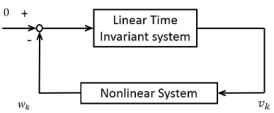
In this section, we study the stability of the proposed adaptation algorithm. In other words, we want to study the convergence property of the tire cornering stiffness estimation error. The energy-based hyperstability approach [31] is used as it addresses the problem nonlinearity. The analysis will follow three steps.

  1. A.

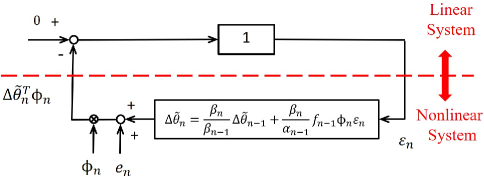
    Formulate the adaptation algorithm (21) as a nonlinear feedback systems shown in Fig. 3 where vksubscript𝑣𝑘v_{k} will be linked to the error between the measured output Yksubscript𝑌𝑘Y_{k} listed in (18) at time k𝑘k and the one predicted according to the adaptation law ΦkTθksuperscriptsubscriptΦ𝑘𝑇subscriptsuperscript𝜃𝑘\Phi_{k}^{T}\theta^{*}_{k}.

  2. B.

    Prove that vksubscript𝑣𝑘v_{k} converges to 00 for k𝑘k\rightarrow\infty by using the sufficient conditions of the hyperstability listed in Appendix A.

  3. C.

    Use the previous results to prove the convergence of the estimated tire cornering stiffnesses to a neighbourhood of the true ones.

IV-A Nonlinear feedback formulation of the adaptation algorithm

We start by formulating the adaptation algorithm (21) as a nonlinear feedback system. We first derive a recursive law for the adaptation gain, (Rk+δI2)1superscriptsubscript𝑅𝑘𝛿subscriptI21(R_{k}+\delta\text{I}_{2})^{-1}. Define Fk=(Rk+δI2)1subscript𝐹𝑘superscriptsubscript𝑅𝑘𝛿subscriptI21F_{k}=(R_{k}+\delta\text{I}_{2})^{-1} and substitute Rksubscript𝑅𝑘R_{k} as defined in (22). We obtain:

Fksubscript𝐹𝑘\displaystyle F_{k} =[λFk11+δ(1λ)I2+ΦkΦkT]1.absentsuperscriptdelimited-[]𝜆superscriptsubscript𝐹𝑘11𝛿1𝜆subscriptI2subscriptΦ𝑘superscriptsubscriptΦ𝑘𝑇1\displaystyle=[\lambda F_{k-1}^{-1}+\delta(1-\lambda)\text{I}_{2}+\Phi_{k}\Phi_{k}^{T}]^{-1}. (23)

Then, denote (σ1,k,𝒖2,k)subscript𝜎1𝑘subscript𝒖2𝑘(\sigma_{1,k},\bm{u}_{2,k}), (σ2,k,𝒖2,k)subscript𝜎2𝑘subscript𝒖2𝑘(\sigma_{2,k},\bm{u}_{2,k}) as the first and the second pairs of the singular value and the left singular vector of the matrix ΦksubscriptΦ𝑘\Phi_{k}. We can rewrite ΦkΦkTsubscriptΦ𝑘superscriptsubscriptΦ𝑘𝑇\Phi_{k}\Phi_{k}^{T} as

ΦkΦkTsubscriptΦ𝑘superscriptsubscriptΦ𝑘𝑇\displaystyle\Phi_{k}\Phi_{k}^{T} =j=12σj,k2𝒖j,k𝒖j,kT=j=12ϕj,kϕj,kTabsentsuperscriptsubscript𝑗12superscriptsubscript𝜎𝑗𝑘2subscript𝒖𝑗𝑘superscriptsubscript𝒖𝑗𝑘𝑇superscriptsubscript𝑗12subscriptbold-italic-ϕ𝑗𝑘superscriptsubscriptbold-italic-ϕ𝑗𝑘𝑇\displaystyle=\sum_{j=1}^{2}\sigma_{j,k}^{2}\bm{u}_{j,k}\bm{u}_{j,k}^{T}=\sum_{j=1}^{2}\bm{\phi}_{j,k}\bm{\phi}_{j,k}^{T}

and further represent δ(1λ)I2+ΦkΦkT𝛿1𝜆subscriptI2subscriptΦ𝑘superscriptsubscriptΦ𝑘𝑇\delta(1-\lambda)\text{I}_{2}+\Phi_{k}\Phi_{k}^{T} as:

δ(1λ)I2+ΦkΦkT=j=12μj,kϕj,kϕj,kT𝛿1𝜆subscriptI2subscriptΦ𝑘superscriptsubscriptΦ𝑘𝑇superscriptsubscript𝑗12subscript𝜇𝑗𝑘subscriptbold-italic-ϕ𝑗𝑘superscriptsubscriptbold-italic-ϕ𝑗𝑘𝑇\displaystyle\delta(1-\lambda)\text{I}_{2}+\Phi_{k}\Phi_{k}^{T}=\sum_{j=1}^{2}\mu_{j,k}\bm{\phi}_{j,k}\bm{\phi}_{j,k}^{T} (24)
with μj,k=σj,k2+δ(1λ)σj,k21for j=1,2.formulae-sequencesubscript𝜇𝑗𝑘superscriptsubscript𝜎𝑗𝑘2𝛿1𝜆superscriptsubscript𝜎𝑗𝑘21for 𝑗12\displaystyle\quad\mu_{j,k}=\frac{\sigma_{j,k}^{2}+\delta(1-\lambda)}{\sigma_{j,k}^{2}}\geq 1\quad\text{for }j=1,2.

Here, μj,ksubscript𝜇𝑗𝑘\mu_{j,k} is guaranteed to be finite and always exist because σj,k>0subscript𝜎𝑗𝑘0\sigma_{j,k}>0. From the expression of ΦkTsubscriptsuperscriptΦ𝑇𝑘\Phi^{T}_{k} in (18), we observe that ΦkTsubscriptsuperscriptΦ𝑇𝑘\Phi^{T}_{k} is always full rank with exception of singular cases which can be easily discarded in real applications. Combing (23) and (24), we obtain a measurement updated law of the adaptation gain by applying the matrix inverse lemma:

Fksubscript𝐹𝑘\displaystyle F_{k} =[λFk11+μ1,kϕ1,kϕ1,kT+μ2,kϕ2,kϕ2,kT]1absentsuperscriptdelimited-[]𝜆superscriptsubscript𝐹𝑘11subscript𝜇1𝑘subscriptbold-italic-ϕ1𝑘superscriptsubscriptbold-italic-ϕ1𝑘𝑇subscript𝜇2𝑘subscriptbold-italic-ϕ2𝑘superscriptsubscriptbold-italic-ϕ2𝑘𝑇1\displaystyle=[\lambda F_{k-1}^{-1}+\mu_{1,k}\bm{\phi}_{1,k}\bm{\phi}_{1,k}^{T}+\mu_{2,k}\bm{\phi}_{2,k}\bm{\phi}_{2,k}^{T}]^{-1}
=FkFkϕ2,kϕ2,kTFkμ2,k1+ϕ2,kTFkϕ2,kabsentsuperscriptsubscript𝐹𝑘superscriptsubscript𝐹𝑘subscriptbold-italic-ϕ2𝑘superscriptsubscriptbold-italic-ϕ2𝑘𝑇superscriptsubscript𝐹𝑘superscriptsubscript𝜇2𝑘1superscriptsubscriptbold-italic-ϕ2𝑘𝑇superscriptsubscript𝐹𝑘subscriptbold-italic-ϕ2𝑘\displaystyle=F_{k}^{\prime}-\frac{F_{k}^{\prime}\bm{\phi}_{2,k}\bm{\phi}_{2,k}^{T}F_{k}^{\prime}}{\mu_{2,k}^{-1}+\bm{\phi}_{2,k}^{T}F_{k}^{\prime}\bm{\phi}_{2,k}} (25)
whereFkwheresuperscriptsubscript𝐹𝑘\displaystyle\text{where}\quad F_{k}^{\prime} =1λ(Fk1Fk1ϕ1,kϕ1,kTFk1λμ1,k1+ϕ1,kTFk1ϕ1,k).absent1𝜆subscript𝐹𝑘1subscript𝐹𝑘1subscriptbold-italic-ϕ1𝑘superscriptsubscriptbold-italic-ϕ1𝑘𝑇subscript𝐹𝑘1𝜆superscriptsubscript𝜇1𝑘1superscriptsubscriptbold-italic-ϕ1𝑘𝑇subscript𝐹𝑘1subscriptbold-italic-ϕ1𝑘\displaystyle=\frac{1}{\lambda}\left(F_{k-1}-\frac{F_{k-1}\bm{\phi}_{1,k}\bm{\phi}_{1,k}^{T}F_{k-1}}{\lambda\mu_{1,k}^{-1}+\bm{\phi}_{1,k}^{T}F_{k-1}\bm{\phi}_{1,k}}\right). (26)

Notice that the updated law of the adaptation gain (25)-(26) contains two parts. First, Fk1subscript𝐹𝑘1F_{k-1} is updated with the first singular vector of the input measurement data, ϕ1,ksubscriptitalic-ϕ1𝑘\phi_{1,k} to yield Fksuperscriptsubscript𝐹𝑘F_{k}^{\prime}. Then Fksuperscriptsubscript𝐹𝑘F_{k}^{\prime} is updated based on the second singular vector, ϕ2,ksubscriptitalic-ϕ2𝑘\phi_{2,k}. For this reason, the original sampling time k=1,,T𝑘1𝑇k=1,...,T is now converted into n=1,,2T𝑛12𝑇n=1,...,2T, where k=n2𝑘𝑛2k=\lceil\frac{n}{2}\rceil. This will allow us to use the hyperstability theorem which is formulated for SISO systems (Appendix A). Substitute (25) into (21) to obtain:

θ~nsubscriptsuperscript~𝜃𝑛\displaystyle\tilde{\theta}^{*}_{n} =θ~n1βn𝒇nϕnϕnTθ~n1+𝒇nϕny~nabsentsubscriptsuperscript~𝜃𝑛1subscript𝛽𝑛subscript𝒇𝑛subscriptbold-italic-ϕ𝑛superscriptsubscriptbold-italic-ϕ𝑛𝑇subscriptsuperscript~𝜃𝑛1subscript𝒇𝑛subscriptbold-italic-ϕ𝑛subscript~𝑦𝑛\displaystyle=\tilde{\theta}^{*}_{n-1}-\beta_{n}\bm{f}_{n}\bm{\phi}_{n}\bm{\phi}_{n}^{T}\tilde{\theta}^{*}_{n-1}+\bm{f}_{n}\bm{\phi}_{n}\tilde{y}_{n}
=θ~n1+𝒇nϕn(y~nβnϕnTθ~n1)absentsubscriptsuperscript~𝜃𝑛1subscript𝒇𝑛subscriptbold-italic-ϕ𝑛subscript~𝑦𝑛subscript𝛽𝑛superscriptsubscriptbold-italic-ϕ𝑛𝑇superscriptsubscript~𝜃𝑛1\displaystyle=\tilde{\theta}^{*}_{n-1}+\bm{f}_{n}\bm{\phi}_{n}(\tilde{y}_{n}-\beta_{n}\bm{\phi}_{n}^{T}\tilde{\theta}_{n-1}^{*}) (27)
where 𝒇n1where superscriptsubscript𝒇𝑛1\displaystyle\text{where }\quad\bm{f}_{n}^{-1} =αn𝒇n11+βnϕnTϕn,𝒇01=0formulae-sequenceabsentsubscript𝛼𝑛superscriptsubscript𝒇𝑛11subscript𝛽𝑛subscriptsuperscriptitalic-ϕ𝑇𝑛subscriptitalic-ϕ𝑛superscriptsubscript𝒇010\displaystyle=\alpha_{n}\bm{f}_{n-1}^{-1}+\beta_{n}\phi^{T}_{n}\phi_{n},~{}~{}~{}~{}\bm{f}_{0}^{-1}=0
𝒇nsubscript𝒇𝑛\displaystyle\bm{f}_{n} =1αn(𝒇n1𝒇n1ϕnϕnT𝒇𝒏𝟏αnβn1+ϕnT𝒇n1ϕn)absent1subscript𝛼𝑛subscript𝒇𝑛1subscript𝒇𝑛1subscriptbold-italic-ϕ𝑛superscriptsubscriptbold-italic-ϕ𝑛𝑇subscript𝒇𝒏1subscript𝛼𝑛superscriptsubscript𝛽𝑛1superscriptsubscriptbold-italic-ϕ𝑛𝑇subscript𝒇𝑛1subscriptbold-italic-ϕ𝑛\displaystyle=\frac{1}{\alpha_{n}}\left(\bm{f}_{n-1}-\frac{\bm{f}_{n-1}\bm{\phi}_{n}\bm{\phi}_{n}^{T}\bm{f_{n-1}}}{\alpha_{n}\beta_{n}^{-1}+\bm{\phi}_{n}^{T}\bm{f}_{n-1}\bm{\phi}_{n}}\right) (28)
y~nsubscript~𝑦𝑛\displaystyle\tilde{y}_{n} =ϕnTθ~n,θ~0=0,α1=1.formulae-sequenceabsentsuperscriptsubscriptitalic-ϕ𝑛𝑇subscript~𝜃𝑛formulae-sequencesuperscriptsubscript~𝜃00subscript𝛼11\displaystyle=\phi_{n}^{T}\tilde{\theta}_{n},~{}~{}~{}~{}~{}\tilde{\theta}_{0}^{*}=0,~{}~{}~{}~{}~{}\alpha_{1}=1.
ϕn={ϕ1,n2,ϕ2,n2,βn={μ1,n2,μ2,n2,αn={λ,if n is odd1,if n is even.formulae-sequencesubscriptbold-italic-ϕ𝑛casessubscriptbold-italic-ϕ1𝑛2otherwisesubscriptbold-italic-ϕ2𝑛2otherwisesubscript𝛽𝑛casessubscript𝜇1𝑛2otherwisesubscript𝜇2𝑛2otherwisesubscript𝛼𝑛cases𝜆if 𝑛 is odd1if 𝑛 is even.\displaystyle\begin{split}\bm{\phi}_{n}&=\begin{cases}\bm{\phi}_{1,\lceil\frac{n}{2}\rceil},&\\ \bm{\phi}_{2,\lceil\frac{n}{2}\rceil},&\end{cases}~{}~{}~{}~{}~{}\beta_{n}=\begin{cases}\mu_{1,\lceil\frac{n}{2}\rceil},&\\ \mu_{2,\lceil\frac{n}{2}\rceil},&\end{cases}\\ \alpha_{n}&=\begin{cases}\lambda,&\quad\text{if }n\text{ is odd}\\ 1,&\quad\text{if }n\text{ is even.}\end{cases}\end{split} (29)

Notice that y~nsubscript~𝑦𝑛\tilde{y}_{n} is the measured output and ϕnTθ~n1superscriptsubscriptbold-italic-ϕ𝑛𝑇superscriptsubscript~𝜃𝑛1\bm{\phi}_{n}^{T}\tilde{\theta}_{n-1}^{*} is the predicted one according to (27). We then define

εnsubscript𝜀𝑛\displaystyle\varepsilon_{n} =y~nβnϕnTθ~nabsentsubscript~𝑦𝑛subscript𝛽𝑛superscriptsubscriptbold-italic-ϕ𝑛𝑇superscriptsubscript~𝜃𝑛\displaystyle=\tilde{y}_{n}-\beta_{n}\bm{\phi}_{n}^{T}\tilde{\theta}_{n}^{*} (30)
εnosubscriptsuperscript𝜀𝑜𝑛\displaystyle\varepsilon^{o}_{n} =y~nβnϕnTθ~n1absentsubscript~𝑦𝑛subscript𝛽𝑛superscriptsubscriptbold-italic-ϕ𝑛𝑇superscriptsubscript~𝜃𝑛1\displaystyle=\tilde{y}_{n}-\beta_{n}\bm{\phi}_{n}^{T}\tilde{\theta}_{n-1}^{*}
Refer to caption
Figure 4: Block diagram of the adaptation algorithm for stability analysis.

as a “scaled” a-posteriori and a “scaled” a-priori predicted measurement errors, respectively. Right multiplying ϕn+1subscriptbold-italic-ϕ𝑛1\bm{\phi}_{n+1} to 𝒇nsubscript𝒇𝑛\bm{f}_{n} in equation (28), we obtain

𝒇nϕn=𝒇n1ϕnαn+βnϕnT𝒇n1ϕnsubscript𝒇𝑛subscriptitalic-ϕ𝑛subscript𝒇𝑛1subscriptbold-italic-ϕ𝑛subscript𝛼𝑛subscript𝛽𝑛superscriptsubscriptbold-italic-ϕ𝑛𝑇subscript𝒇𝑛1subscriptbold-italic-ϕ𝑛\displaystyle\bm{f}_{n}\phi_{n}=\frac{\bm{f}_{n-1}\bm{\phi}_{n}}{\alpha_{n}+\beta_{n}\bm{\phi}_{n}^{T}\bm{f}_{n-1}\bm{\phi}_{n}} (31)

and the adaptation law (27) becomes

θ~n=θ~n1+𝒇n1ϕnαn+βnϕnT𝒇n1ϕnεno.subscriptsuperscript~𝜃𝑛subscriptsuperscript~𝜃𝑛1subscript𝒇𝑛1subscriptbold-italic-ϕ𝑛subscript𝛼𝑛subscript𝛽𝑛superscriptsubscriptbold-italic-ϕ𝑛𝑇subscript𝒇𝑛1subscriptbold-italic-ϕ𝑛subscriptsuperscript𝜀𝑜𝑛\displaystyle\tilde{\theta}^{*}_{n}=\tilde{\theta}^{*}_{n-1}+\frac{\bm{f}_{n-1}\bm{\phi}_{n}}{\alpha_{n}+\beta_{n}\bm{\phi}_{n}^{T}\bm{f}_{n-1}\bm{\phi}_{n}}\varepsilon^{o}_{n}. (32)

Then, again left multiplying βnϕnTsubscript𝛽𝑛superscriptsubscriptbold-italic-ϕ𝑛𝑇-\beta_{n}\bm{\phi}_{n}^{T} to (32) and adding y~nsubscript~𝑦𝑛\tilde{y}_{n} to both sides of the equation lead to:

εn=αnαn+βnϕnT𝒇n1ϕnεno.subscript𝜀𝑛subscript𝛼𝑛subscript𝛼𝑛subscript𝛽𝑛superscriptsubscriptbold-italic-ϕ𝑛𝑇subscript𝒇𝑛1subscriptbold-italic-ϕ𝑛subscriptsuperscript𝜀𝑜𝑛\displaystyle\varepsilon_{n}=\frac{\alpha_{n}}{\alpha_{n}+\beta_{n}\bm{\phi}_{n}^{T}\bm{f}_{n-1}\bm{\phi}_{n}}\varepsilon^{o}_{n}. (33)

With this relation, we can express the adaptation law (32) using the a-posteriori predicted measurement error εnsubscript𝜀𝑛\varepsilon_{n} as follows:

θ~n=θ~n1+1αn𝒇n1ϕnεn.subscriptsuperscript~𝜃𝑛subscriptsuperscript~𝜃𝑛11subscript𝛼𝑛subscript𝒇𝑛1subscriptbold-italic-ϕ𝑛subscript𝜀𝑛\displaystyle\tilde{\theta}^{*}_{n}=\tilde{\theta}^{*}_{n-1}+\frac{1}{\alpha_{n}}\bm{f}_{n-1}\bm{\phi}_{n}\varepsilon_{n}. (34)

Define the “scaled” parameter estimation error as

Δθ~n=βnθ~nθ~n,Δsubscript~𝜃𝑛subscript𝛽𝑛subscriptsuperscript~𝜃𝑛subscript~𝜃𝑛\displaystyle\Delta\tilde{\theta}_{n}=\beta_{n}\tilde{\theta}^{*}_{n}-\tilde{\theta}_{n}, (35)

with θ~0=0subscript~𝜃00\tilde{\theta}_{0}=0 and β0=1subscript𝛽01\beta_{0}=1. We can rewrite (30) and (34)-(35) into the following error dynamics:

{εn=ϕnTθ~nβnϕnTθ~n=ϕnTΔθ~nΔθ~n=βnβn1Δθ~n1+βnαn1𝒇n1ϕnεn+encasessubscript𝜀𝑛subscriptsuperscriptitalic-ϕ𝑇𝑛subscript~𝜃𝑛subscript𝛽𝑛superscriptsubscriptbold-italic-ϕ𝑛𝑇superscriptsubscript~𝜃𝑛subscriptsuperscriptitalic-ϕ𝑇𝑛Δsubscript~𝜃𝑛otherwiseΔsubscript~𝜃𝑛subscript𝛽𝑛subscript𝛽𝑛1Δsubscript~𝜃𝑛1subscript𝛽𝑛subscript𝛼𝑛1subscript𝒇𝑛1subscriptitalic-ϕ𝑛subscript𝜀𝑛subscript𝑒𝑛otherwise\displaystyle\begin{cases}\varepsilon_{n}=\phi^{T}_{n}\tilde{\theta}_{n}-\beta_{n}\bm{\phi}_{n}^{T}\tilde{\theta}_{n}^{*}=-\phi^{T}_{n}\Delta\tilde{\theta}_{n}\\ \Delta\tilde{\theta}_{n}=\frac{\beta_{n}}{\beta_{n-1}}\Delta\tilde{\theta}_{n-1}+\frac{\beta_{n}}{\alpha_{n-1}}\bm{f}_{n-1}\phi_{n}\varepsilon_{n}+e_{n}\end{cases} (36)

where en=βnβn1θ~n1θ~nsubscript𝑒𝑛subscript𝛽𝑛subscript𝛽𝑛1subscript~𝜃𝑛1subscript~𝜃𝑛e_{n}=\frac{\beta_{n}}{\beta_{n-1}}\tilde{\theta}_{n-1}-\tilde{\theta}_{n} is treated as an external bounded disturbance. Finally, we can represent this error dynamics into the block diagram of Fig. 4 which is equivalent to the nonlinear feedback system as shown in Fig. 3.

IV-B Hyperstability analysis

Theorem IV.1.
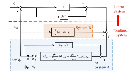
The nonlinear feedback system depicted in the block diagram of Fig. 4 with the error dynamics described in (36) without the external disturbance term ensubscript𝑒𝑛e_{n} is asymptotically hyperstable (i.e. εn0subscript𝜀𝑛0\varepsilon_{n}\rightarrow 0) if

2αn+1βn1βn10n=1,2,.formulae-sequence2subscript𝛼𝑛1subscript𝛽𝑛1subscript𝛽𝑛10for-all𝑛12\displaystyle\frac{2-\alpha_{n+1}}{\beta_{n}}-\frac{1}{\beta_{n-1}}\geq 0\quad\forall n=1,2,...\infty. (37)
Refer to caption
Figure 5: Equivalent system of the block diagram in Fig. 4 for stability analysis.
Proof.

To prove the theorem we use the concept of hyperstability [31] briefly summarized in Appendix A. Next, we prove that the sufficient conditions listed in Theorem A.1 are satisfied. First, we notice that the forward linear system is the identity, which is obviously strictly positive real. However, the nonlinear block of the adaptation algorithm does not satisfy the Popov inequality. Therefore, we further modify the system and rewrite it as the one shown in the block diagram of Fig. 5. Since the same signals have been added and subtracted in the feedback system, the stability property will not change.

We now again check the sufficient conditions for the modified system. Start with the requirement of the nonlinear feedback block satisfying Popov inequality. Considering System A in the block diagram of Fig. 5 with input (snsubscript𝑠𝑛s_{n}) and output (wnsubscript𝑤𝑛w_{n}) signals, we have

wnsubscript𝑤𝑛\displaystyle w_{n} =Δθ~nTϕn,sn=εn+αn+12Δθ~nTϕnformulae-sequenceabsentΔsubscriptsuperscript~𝜃𝑇𝑛subscriptbold-italic-ϕ𝑛subscript𝑠𝑛subscript𝜀𝑛subscript𝛼𝑛12Δsubscriptsuperscript~𝜃𝑇𝑛subscriptbold-italic-ϕ𝑛\displaystyle=\Delta\tilde{\theta}^{T}_{n}\bm{\phi}_{n},~{}~{}s_{n}=\varepsilon_{n}+\frac{\alpha_{n+1}}{2}\Delta\tilde{\theta}^{T}_{n}\bm{\phi}_{n}
ϕnϕnTsubscriptbold-italic-ϕ𝑛superscriptsubscriptbold-italic-ϕ𝑛𝑇\displaystyle\bm{\phi}_{n}\bm{\phi}_{n}^{T} =βn1(𝒇n1αn𝒇n11)absentsuperscriptsubscript𝛽𝑛1superscriptsubscript𝒇𝑛1subscript𝛼𝑛superscriptsubscript𝒇𝑛11\displaystyle=\beta_{n}^{-1}(\bm{f}_{n}^{-1}-\alpha_{n}\bm{f}_{n-1}^{-1})
ϕnεnsubscriptbold-italic-ϕ𝑛subscript𝜀𝑛\displaystyle\bm{\phi}_{n}\varepsilon_{n} =αnβn𝒇n11Δθ~nαnβn1𝒇n11Δθ~n1absentsubscript𝛼𝑛subscript𝛽𝑛superscriptsubscript𝒇𝑛11Δsubscript~𝜃𝑛subscript𝛼𝑛subscript𝛽𝑛1superscriptsubscript𝒇𝑛11Δsubscript~𝜃𝑛1\displaystyle=\frac{\alpha_{n}}{\beta_{n}}\bm{f}_{n-1}^{-1}\Delta\tilde{\theta}_{n}-\frac{\alpha_{n}}{\beta_{n-1}}\bm{f}_{n-1}^{-1}\Delta\tilde{\theta}_{n-1} (38)

from equations (28) and (36) without considering the external disturbanceensubscript𝑒𝑛e_{n}. Define

ηn=2αn+1βn1βn1subscript𝜂𝑛2subscript𝛼𝑛1subscript𝛽𝑛1subscript𝛽𝑛1\displaystyle\eta_{n}=\frac{2-\alpha_{n+1}}{\beta_{n}}-\frac{1}{\beta_{n-1}}

for the sake of simplicity in later expression. The sum of the product of wnsubscript𝑤𝑛w_{n} and snsubscript𝑠𝑛s_{n} can be calculated as:

n=12kwnsn=n=12kΔθ~nTϕn(εn+αn+12Δθ~nTϕn)superscriptsubscript𝑛12𝑘subscript𝑤𝑛subscript𝑠𝑛superscriptsubscript𝑛12𝑘Δsubscriptsuperscript~𝜃𝑇𝑛subscriptbold-italic-ϕ𝑛subscript𝜀𝑛subscript𝛼𝑛12Δsubscriptsuperscript~𝜃𝑇𝑛subscriptbold-italic-ϕ𝑛\displaystyle\sum_{n=1}^{2k}w_{n}s_{n}=\sum_{n=1}^{2k}\Delta\tilde{\theta}^{T}_{n}\bm{\phi}_{n}(\varepsilon_{n}+\frac{\alpha_{n+1}}{2}\Delta\tilde{\theta}^{T}_{n}\bm{\phi}_{n})
=\displaystyle= n=12kαn21βn1(Δθ~nTΔθ~n1T)𝒇n11(Δθ~nΔθ~n1)superscriptsubscript𝑛12𝑘subscript𝛼𝑛21subscript𝛽𝑛1Δsuperscriptsubscript~𝜃𝑛𝑇Δsuperscriptsubscript~𝜃𝑛1𝑇superscriptsubscript𝒇𝑛11Δsubscript~𝜃𝑛Δsubscript~𝜃𝑛1\displaystyle\sum_{n=1}^{2k}\frac{\alpha_{n}}{2}\frac{1}{\beta_{n-1}}(\Delta\tilde{\theta}_{n}^{T}-\Delta\tilde{\theta}_{n-1}^{T})\bm{f}_{n-1}^{-1}(\Delta\tilde{\theta}_{n}-\Delta\tilde{\theta}_{n-1})
+n=12kαn+12βnΔθ~nT𝒇n1Δθ~nαn2βn1Δθ~n1T𝒇n11Δθ~n1superscriptsubscript𝑛12𝑘subscript𝛼𝑛12subscript𝛽𝑛Δsubscriptsuperscript~𝜃𝑇𝑛superscriptsubscript𝒇𝑛1Δsubscript~𝜃𝑛subscript𝛼𝑛2subscript𝛽𝑛1Δsubscriptsuperscript~𝜃𝑇𝑛1superscriptsubscript𝒇𝑛11Δsubscript~𝜃𝑛1\displaystyle~{}~{}+\sum_{n=1}^{2k}\frac{\alpha_{n+1}}{2\beta_{n}}\Delta\tilde{\theta}^{T}_{n}\bm{f}_{n}^{-1}\Delta\tilde{\theta}_{n}-\frac{\alpha_{n}}{2\beta_{n-1}}\Delta\tilde{\theta}^{T}_{n-1}\bm{f}_{n-1}^{-1}\Delta\tilde{\theta}_{n-1}
+n=02kηnαn2Δθ~nT𝒇n11Δθ~nsuperscriptsubscript𝑛02𝑘subscript𝜂𝑛subscript𝛼𝑛2Δsuperscriptsubscript~𝜃𝑛𝑇superscriptsubscript𝒇𝑛11Δsubscript~𝜃𝑛\displaystyle~{}~{}~{}~{}~{}~{}~{}~{}+\sum_{n=0}^{2k}\frac{\eta_{n}\alpha_{n}}{2}\Delta\tilde{\theta}_{n}^{T}\bm{f}_{n-1}^{-1}\Delta\tilde{\theta}_{n}
=\displaystyle= n=12kαn2βn1(Δθ~nTΔθ~n1T)𝒇n11(Δθ~nΔθ~n1)superscriptsubscript𝑛12𝑘subscript𝛼𝑛2subscript𝛽𝑛1Δsuperscriptsubscript~𝜃𝑛𝑇Δsuperscriptsubscript~𝜃𝑛1𝑇superscriptsubscript𝒇𝑛11Δsubscript~𝜃𝑛Δsubscript~𝜃𝑛1\displaystyle\sum_{n=1}^{2k}\frac{\alpha_{n}}{2\beta_{n-1}}(\Delta\tilde{\theta}_{n}^{T}-\Delta\tilde{\theta}_{n-1}^{T})\bm{f}_{n-1}^{-1}(\Delta\tilde{\theta}_{n}-\Delta\tilde{\theta}_{n-1})
+α2k+12β2kΔθ~2kT𝒇2k1Δθ~2kα12β0Δθ~0T𝒇01Δθ~0subscript𝛼2𝑘12subscript𝛽2𝑘Δsubscriptsuperscript~𝜃𝑇2𝑘superscriptsubscript𝒇2𝑘1Δsubscript~𝜃2𝑘subscript𝛼12subscript𝛽0Δsubscriptsuperscript~𝜃𝑇0superscriptsubscript𝒇01Δsubscript~𝜃0\displaystyle~{}~{}~{}~{}~{}~{}~{}~{}+\frac{\alpha_{2k+1}}{2\beta_{2k}}\Delta\tilde{\theta}^{T}_{2k}\bm{f}_{2k}^{-1}\Delta\tilde{\theta}_{2k}-\frac{\alpha_{1}}{2\beta_{0}}\Delta\tilde{\theta}^{T}_{0}\bm{f}_{0}^{-1}\Delta\tilde{\theta}_{0}
+n=12kηnαn2Δθ~nT𝒇n11Δθ~n.superscriptsubscript𝑛12𝑘subscript𝜂𝑛subscript𝛼𝑛2Δsuperscriptsubscript~𝜃𝑛𝑇superscriptsubscript𝒇𝑛11Δsubscript~𝜃𝑛\displaystyle~{}~{}~{}~{}~{}~{}~{}~{}~{}~{}~{}~{}+\sum_{n=1}^{2k}\frac{\eta_{n}\alpha_{n}}{2}\Delta\tilde{\theta}_{n}^{T}\bm{f}_{n-1}^{-1}\Delta\tilde{\theta}_{n}. (39)

Since all the variables of αnsubscript𝛼𝑛\alpha_{n}, βnsubscript𝛽𝑛\beta_{n} are positive as defined in (29), we can know that the sum of the product of wnsubscript𝑤𝑛w_{n} and snsubscript𝑠𝑛s_{n} will have a lower bound

TABLE I: Model Parameters
vehicle mass m𝑚m 2300.132 kg
vehicle rotational inertia Izsubscript𝐼𝑧I_{z} 4400 kgm2
distance from COG to front axle Lfsubscript𝐿𝑓L_{f} 1.505 m
distance from COG to rear axle Lrsubscript𝐿𝑟L_{r} 1.504 m
front tire conering stiffness Cfsubscript𝐶𝑓C_{f} 160776 N/rad2
rear tire conering stiffness Crsubscript𝐶𝑟C_{r} 254100 N/rad2
gravity g𝑔g 9.80665 m/s2
n=12kwnsnsuperscriptsubscript𝑛12𝑘subscript𝑤𝑛subscript𝑠𝑛absent\displaystyle\sum_{n=1}^{2k}w_{n}s_{n}\geq α12β0Δθ~0T𝒇01Δθ~0=0subscript𝛼12subscript𝛽0Δsubscriptsuperscript~𝜃𝑇0superscriptsubscript𝒇01Δsubscript~𝜃00\displaystyle-\frac{\alpha_{1}}{2\beta_{0}}\Delta\tilde{\theta}^{T}_{0}\bm{f}_{0}^{-1}\Delta\tilde{\theta}_{0}=0

and satisfy the Pupov inequality with a condition of

ηn0n=1,2,,2k.formulae-sequencesubscript𝜂𝑛0for-all𝑛122𝑘\displaystyle\eta_{n}\geq 0\quad\forall n=1,2,...,2k. (40)

Next, considering the time varying linear System B in the block diagram of Fig. 5, we find that it also satisfies the Popov inequality since

12(ραn+1)0for choosing 1ρ<2.formulae-sequence12𝜌subscript𝛼𝑛10for choosing 1𝜌2\displaystyle\frac{1}{2}(\rho-\alpha_{n+1})\geq 0\quad\text{for choosing }~{}1\leq\rho<2. (41)

Then, the overall nonlinear feedback system as shown in the block diagram of Fig. 5 satisfies the Popov inequality since it is made by a feedback connection of two passive systems, A and B. Finally, the linear feedforward system for the modified system, 1ρ/21𝜌21-\rho/2, is strictly positive real for having 1ρ<21𝜌21\leq\rho<2. Now, we know that the adaptation system is hyperstable. In other words, |(1ρ/2)wn|<1𝜌2subscript𝑤𝑛|(1-\rho/2)w_{n}|<\infty is bounded. This will further imply that the output of the nonlinear feedback system, wn<subscript𝑤𝑛w_{n}<\infty, is bounded as well. Therefore, having all of three requirements listed in Appendix A, we can conclude that the adaptation system without the external disturbance is asymptotic hyperstable εn0subscript𝜀𝑛0\varepsilon_{n}\rightarrow 0. ∎

We start from the analysis in Theorem V.1 and consider the effect of the external disturbance ensubscript𝑒𝑛e_{n}.

Theorem IV.2.

Assume that the two norm of the difference of the true parameter θ~ksubscript~𝜃𝑘\tilde{\theta}_{k} between two consecutive steps is bounded:

θ~k1θ~k2Λk=1,2,,.formulae-sequencesubscriptnormsubscript~𝜃𝑘1subscript~𝜃𝑘2Λfor-all𝑘12\displaystyle\|\tilde{\theta}_{k-1}-\tilde{\theta}_{k}\|_{2}\leq\Lambda~{}~{}~{}~{}\quad\forall k=1,2,...,\infty.

Consider the regularized weighted least square problem (19) with the regression model described in (18). Then, there exists a set of parameters δ>0,0λ<1formulae-sequence𝛿0much-less-than0𝜆1\delta>0,0\ll\lambda<1 satisfying the condition:

σ1,k2σ2,k2+δ(2λ)σ2,k2δσ1,k20k=1,2,,formulae-sequencesuperscriptsubscript𝜎1𝑘2superscriptsubscript𝜎2𝑘2𝛿2𝜆superscriptsubscript𝜎2𝑘2𝛿superscriptsubscript𝜎1𝑘20for-all𝑘12\displaystyle\sigma_{1,k}^{2}\sigma_{2,k}^{2}+\delta(2-\lambda)\sigma_{2,k}^{2}-\delta\sigma_{1,k}^{2}\geq 0~{}~{}\forall k=1,2,...,\infty (42)

which guarantees ε2kR(Λ)subscript𝜀2𝑘𝑅Λ\varepsilon_{2k}\in R(\Lambda) for R(Λ)𝑅ΛR(\Lambda) being a ball of radius ΛΛ\Lambda centred in the origin.

Proof.

We use the same steps as in Theorem V.1. Consider the input signal εnsubscript𝜀𝑛\varepsilon_{n} of System A with

ϕnεn=αnβn𝒇n11(Δθ~n+\displaystyle\phi_{n}\varepsilon_{n}=\frac{\alpha_{n}}{\beta_{n}}\bm{f}_{n-1}^{-1}(\Delta\tilde{\theta}_{n}+ θ~n)αnβn1𝒇n11(Δθ~n1+θ~n1)\displaystyle\tilde{\theta}_{n})-\frac{\alpha_{n}}{\beta_{n-1}}\bm{f}_{n-1}^{-1}(\Delta\tilde{\theta}_{n-1}+\tilde{\theta}_{n-1})

deriving from (36). We can derive the same Popov inequality as shown in (39) for System A but with an extra term of

n=12kαnΔθ~nT𝒇n11(1βnθ~n1βn1θ~n1).superscriptsubscript𝑛12𝑘subscript𝛼𝑛Δsuperscriptsubscript~𝜃𝑛𝑇superscriptsubscript𝒇𝑛111subscript𝛽𝑛subscript~𝜃𝑛1subscript𝛽𝑛1subscript~𝜃𝑛1\displaystyle\sum_{n=1}^{2k}\alpha_{n}\Delta\tilde{\theta}_{n}^{T}\bm{f}_{n-1}^{-1}(\frac{1}{\beta_{n}}\tilde{\theta}_{n}-\frac{1}{\beta_{n-1}}\tilde{\theta}_{n-1}). (43)

Therefore, the same requirement of ηn=2αn+1βn1βn10subscript𝜂𝑛2subscript𝛼𝑛1subscript𝛽𝑛1subscript𝛽𝑛10\eta_{n}=\frac{2-\alpha_{n+1}}{\beta_{n}}-\frac{1}{\beta_{n-1}}\geq 0 in Theorem V.1 is necessary for hyperstability. From this, we can easily infer the condition of (42) by expanding out βn1subscript𝛽𝑛1\beta_{n-1}, βnsubscript𝛽𝑛\beta_{n} and αn+1subscript𝛼𝑛1\alpha_{n+1} using (29).

TABLE II: Estimator Parameters (Algorithm 1)
sampling time ΔtΔ𝑡\Delta t 0.01 sec
covariance matrix of wk[k]subscript𝑤𝑘delimited-[]𝑘w_{k}[k] Wksubscript𝑊𝑘W_{k} diag([0.2,0.6,0.05])0.20.60.05([0.2,0.6,0.05])
covariance matrix of vk[k]subscript𝑣𝑘delimited-[]𝑘v_{k}[k] Vksubscript𝑉𝑘V_{k} 0.05
covariance matrix of wd[k]subscript𝑤𝑑delimited-[]𝑘w_{d}[k] Wdsubscript𝑊𝑑W_{d} diag([6,0.5,0.1,0.0002])60.50.10.0002([6,0.5,0.1,0.0002])
covariance matrix of vd[k]subscript𝑣𝑑delimited-[]𝑘v_{d}[k] Vdsubscript𝑉𝑑V_{d} diag([0.1,0.01])0.10.01([0.1,0.01])
forgetting factor λ𝜆\lambda 0.975
regularized term weighting δ𝛿\delta 0.02
yaw rate threshold rtsubscript𝑟𝑡r_{t} 0.1 rad/srads\text{rad}/\text{s}

Next, combining the first term in the right hand side of (39) together with (43), we can conclude that System A will satisfy Pupov inequality under the conditions:

ηn2Δθ~nT𝒇n11Δθ~n+Δθ~nT𝒇n11subscript𝜂𝑛2Δsuperscriptsubscript~𝜃𝑛𝑇superscriptsubscript𝒇𝑛11Δsubscript~𝜃𝑛Δsuperscriptsubscript~𝜃𝑛𝑇superscriptsubscript𝒇𝑛11\displaystyle\frac{\eta_{n}}{2}\Delta\tilde{\theta}_{n}^{T}\bm{f}_{n-1}^{-1}\Delta\tilde{\theta}_{n}+\Delta\tilde{\theta}_{n}^{T}\bm{f}_{n-1}^{-1} (1βnθ~n1βn1θ~n1)01subscript𝛽𝑛subscript~𝜃𝑛1subscript𝛽𝑛1subscript~𝜃𝑛10\displaystyle(\frac{1}{\beta_{n}}\tilde{\theta}_{n}-\frac{1}{\beta_{n-1}}\tilde{\theta}_{n-1})\geq 0
n=1,2,,2kfor-all𝑛122𝑘\displaystyle\quad\quad\forall n=1,2,...,2k
Δθ~n22κ(𝒇n11)ηnabsentsubscriptnormΔsubscript~𝜃𝑛22𝜅superscriptsubscript𝒇𝑛11subscript𝜂𝑛\displaystyle\implies\|\Delta\tilde{\theta}_{n}\|_{2}\geq\frac{2\kappa(\bm{f}_{n-1}^{-1})}{\eta_{n}} 1βnθ~n1βn1θ~n12subscriptnorm1subscript𝛽𝑛subscript~𝜃𝑛1subscript𝛽𝑛1subscript~𝜃𝑛12\displaystyle\left\|\frac{1}{\beta_{n}}\tilde{\theta}_{n}-\frac{1}{\beta_{n-1}}\tilde{\theta}_{n-1}\right\|_{2}
n=1,2,,2kfor-all𝑛122𝑘\displaystyle\quad\quad\forall n=1,2,...,2k (44)

where κ()𝜅\kappa(\cdot) denotes the condition number of the positive definite matrix 𝒇n11superscriptsubscript𝒇𝑛11\bm{f}_{n-1}^{-1}. Since the rate of θ~~𝜃\tilde{\theta} is bounded by the assumption, the existence of the right hand side in (44) is guaranteed. Then, based on passivity theorem [32], we know that there exists a time-varying energy function which is positive definite and is dissipating over time in the region of

Δθ~2maxn2κ(𝒇n11)ηn1βnθ~n1βn1θ~n12.subscriptnormΔ~𝜃2subscript𝑛2𝜅superscriptsubscript𝒇𝑛11subscript𝜂𝑛subscriptnorm1subscript𝛽𝑛subscript~𝜃𝑛1subscript𝛽𝑛1subscript~𝜃𝑛12\displaystyle\|\Delta\tilde{\theta}\|_{2}\geq\max_{n}\frac{2\kappa(\bm{f}_{n-1}^{-1})}{\eta_{n}}\left\|\frac{1}{\beta_{n}}\tilde{\theta}_{n}-\frac{1}{\beta_{n-1}}\tilde{\theta}_{n-1}\right\|_{2}. (45)

Equation (45) implies the boundedness of the predicted measurement error ϵnsubscriptitalic-ϵ𝑛\epsilon_{n} in the adaptation algorithm. ∎

Remark: Some considerations can be drawn from the analysis in Theorem V.1 and Theorem V.2. First, the boundedness of the adaptation error depends on the time-varying rate of change of θ~~𝜃\tilde{\theta}. According to the result shown in (45), a larger value in 1βnθ~n1βn1θ~n12subscriptnorm1subscript𝛽𝑛subscript~𝜃𝑛1subscript𝛽𝑛1subscript~𝜃𝑛12\left\|\frac{1}{\beta_{n}}\tilde{\theta}_{n}-\frac{1}{\beta_{n-1}}\tilde{\theta}_{n-1}\right\|_{2} will lead to a larger bound in the predicted measurement error. Therefore, we can expect a better adaptation performance under non-extreme driving scenarios. Second, the boundedness of the adaptation error shrinks as the condition number of 𝒇n11superscriptsubscript𝒇𝑛11\bm{f}_{n-1}^{-1} decreases. This highlights the importance of input measurement matrices, ΦiTsubscriptsuperscriptΦ𝑇𝑖\Phi^{T}_{i}, being well-conditioned in the regression model. By observing (18), we can infer that the conditional number of ΦTsuperscriptΦ𝑇\Phi^{T} is roughly equal to the ratio of it’s (2, 1) and (2, 2) components, since LfLrsubscript𝐿𝑓subscript𝐿𝑟L_{f}\approx L_{r} for a vehicle. In order to avoid a bad adaptation performance, we should add an additional condition of
Refer to caption
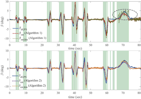
Figure 6: Performance comparison of Algorithm 1 and Algorithm 2 for a slalom test.
1ct|ΦT(2,1)ΦT(2,2)|ct1subscript𝑐𝑡superscriptΦ𝑇21superscriptΦ𝑇22subscript𝑐𝑡\displaystyle\frac{1}{c_{t}}\leq\left|\frac{\Phi^{T}(2,1)}{\Phi^{T}(2,2)}\right|\leq c_{t} (46)

to enable the adaptation process in our proposed sideslip angle algorithm where ct>0subscript𝑐𝑡0c_{t}>0 is the maximum allowed conditional number of measurement data. Third, according to (39), ηnsubscript𝜂𝑛\eta_{n} is the energy dissipation rate of the system. Therefore, a larger value of ηnsubscript𝜂𝑛\eta_{n} results in a faster convergence rate. Based on an further analysis in the condition of ηn0subscript𝜂𝑛0\eta_{n}\geq 0, we can obtain a good starting value of the regularization weight

δ1/(1σ2,k21σ1,k2)𝛿/11superscriptsubscript𝜎2𝑘21superscriptsubscript𝜎1𝑘2\displaystyle\delta\approx 1\left/\right.(\frac{1}{\sigma_{2,k}^{2}}-\frac{1}{\sigma_{1,k}^{2}}) (47)

This is derived by rewriting (42) into the following form:

2λσ1,k2(1σ2,k21δ)for 0λ<1.formulae-sequence2𝜆superscriptsubscript𝜎1𝑘21superscriptsubscript𝜎2𝑘21𝛿much-less-thanfor 0𝜆1\displaystyle 2-\lambda\geq\sigma_{1,k}^{2}\left(\frac{1}{\sigma_{2,k}^{2}}-\frac{1}{\delta}\right)\quad\text{for ~{}}0\ll\lambda<1. (48)

IV-C Convergence of the estimated cornering stiffness

Theorem IV.3.

The asymptotical hyperstability of the nonlinear feedback system depicted in Fig. 4 with en=0subscript𝑒𝑛0e_{n}=0 guarantees that the estimated parameters converge to 1βnθ~n1subscript𝛽𝑛subscript~𝜃𝑛\frac{1}{\beta_{n}}\tilde{\theta}_{n}

limnθ~n1βnθ~nsubscript𝑛superscriptsubscript~𝜃𝑛1subscript𝛽𝑛subscript~𝜃𝑛\displaystyle\lim_{n\rightarrow\infty}\tilde{\theta}_{n}^{*}\rightarrow\frac{1}{\beta_{n}}\tilde{\theta}_{n}
Proof.

In Theorem V.1, the stability proof shows the convergence of εnsubscript𝜀𝑛\varepsilon_{n} without the disturbance term.

εnsubscript𝜀𝑛\displaystyle\varepsilon_{n} =ϕnT(θ~nβnθ~n)0.absentsubscriptsuperscriptbold-italic-ϕ𝑇𝑛subscript~𝜃𝑛subscript𝛽𝑛superscriptsubscript~𝜃𝑛0\displaystyle=\bm{\phi}^{T}_{n}(\tilde{\theta}_{n}-\beta_{n}\tilde{\theta}_{n}^{*})\rightarrow 0. (49)

Then, recalling from (33), we know that εn0superscriptsubscript𝜀𝑛0\varepsilon_{n}^{0} will also converge to zero for a bounded ϕnsubscriptbold-italic-ϕ𝑛\bm{\phi}_{n}. We have

εn+10superscriptsubscript𝜀𝑛10\displaystyle\varepsilon_{n+1}^{0} =ϕn+1T(θ~n+1βn+1θ~n)0absentsubscriptsuperscriptbold-italic-ϕ𝑇𝑛1subscript~𝜃𝑛1subscript𝛽𝑛1superscriptsubscript~𝜃𝑛0\displaystyle=\bm{\phi}^{T}_{n+1}(\tilde{\theta}_{n+1}-\beta_{n+1}\tilde{\theta}_{n}^{*})\rightarrow 0

which can be further rewritten as

ϕn+1T(θ~nβnθ~n)0subscriptsuperscriptbold-italic-ϕ𝑇𝑛1subscript~𝜃𝑛subscript𝛽𝑛superscriptsubscript~𝜃𝑛0\displaystyle\bm{\phi}^{T}_{n+1}(\tilde{\theta}_{n}-\beta_{n}\tilde{\theta}_{n}^{*})\rightarrow 0 (50)

by substituting θ~n+1=βn+1βnθ~nsubscript~𝜃𝑛1subscript𝛽𝑛1subscript𝛽𝑛subscript~𝜃𝑛\tilde{\theta}_{n+1}=\frac{\beta_{n+1}}{\beta_{n}}\tilde{\theta}_{n} under the assumption of no external disturbance.

Combining the results of (49) and (50) and using the fact that θ~nβnθ~nsubscript~𝜃𝑛subscript𝛽𝑛superscriptsubscript~𝜃𝑛\tilde{\theta}_{n}-\beta_{n}\tilde{\theta}_{n}^{*} cannot be orthogonal to ϕnsubscriptbold-italic-ϕ𝑛\bm{\phi}_{n} and ϕn+1subscriptbold-italic-ϕ𝑛1\bm{\phi}_{n+1} since ϕnsubscriptbold-italic-ϕ𝑛\bm{\phi}_{n} and ϕn+1subscriptbold-italic-ϕ𝑛1\bm{\phi}_{n+1} span the whole state space, we can conclude that θ~nβnθ~nsubscript~𝜃𝑛subscript𝛽𝑛superscriptsubscript~𝜃𝑛\tilde{\theta}_{n}-\beta_{n}\tilde{\theta}_{n}^{*} will approach zero as n𝑛n\rightarrow\infty. ∎

From Theorem V.2 and Theorem V.3 we can conclude that the estimated tire cornering stiffness coefficients will converge to a neighbourhood of the true values when we include the external disturbance ensubscript𝑒𝑛e_{n} term in the proof.

Refer to caption
Figure 7: Performance comparison of Algorithm 1 and Algorithm 2 for a severe single lane changing.

V Algorithm Improvement

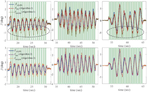
In this section, the proposed estimation algorithm is evaluated with real experimental tests. We first conducted a slalom and a severe single lane changing tests at Hyundai-Kia Motors California Proving Ground. The first test setting consists of eleven lined up cones, separated by 18 m. The vehicle is driven through the course in a slalom pattern at constant speed, 50 km/hr. The second one is a standardized maneuver which generates a peak lateral acceleration of approximately 0.6g. A further analysis and a small modification of Algorithm 1 are provided based on the estimation results.

V-A Experimental Setup

Our experimental vehicle is a 5thsuperscript5𝑡5^{th} generation Hyundai Genesis equipped with a differential global positioning system (dGPS) Oxford TR3000. A real-time kinematics (RTK) technology is adopted to allow an accuracy down to 2-4 cm for position measurement. We will consider the measured sideslip angle provided from dGSP as a ground truth to validate the estimated performance. The real–time computations are performed on a dSPACE DS1401 Autobox system which consists of a IBM PowerPC 750GL processor running at 900 MHz. The aforementioned hardware components communicate through a CAN bus and the estimation algorithm is executed at 100 Hz.

Table I shows the nominal model parameters of the test vehicle and Table II shows the estimation parameters for Algorithm 1. We initialize the measurement noise covariances by processing the measurement outputs while they are held constant. Since the values of the noise covariances are all small, we then apply a reasonable scaling factor to avoid the numerical issue before the tuning. The process noise covariance matrix is picked based on the unmodeled dynamics. According to the results shown in Table II, we can see that the process noise covariance of the vysubscript𝑣𝑦v_{y} equation is chosen to be relative bigger than other states since the coupling of the roll dynamics has been ignored and the gravity effect causes more influence on vysubscript𝑣𝑦v_{y} dynamics. Similarly, we choose the process noise covariance of the sensor bias, d𝑑d, to be significantly small because we believe that the offset is “nearly” constant. In other words, we can treat the dynamics of d𝑑d as arbitrarily-slowly time-varying. For the forgetting factor, since it determines the rate of change of the weighting factors of the regression errors, we start with the value vary close to 1 for the fact that the tire cornering stiffness varies with the maneuver and our sampling rate is way fast enough to capture its varying speed. Then, we gradually decrease the value to allow more weighting on recent data to improve the performance.
Refer to caption
Figure 8: The root mean square errors of the proposed method compared with the existing methods.

V-B Motivation

The estimation results of a slalom and a severe single lane changing tests are shown in the upper plots of Fig. 6 and Fig. 7 respectively. Note that the light green background represents the condition of |r|>rt𝑟subscript𝑟𝑡|r|>r_{t} indicating that the adaptation algorithm is active. Comparing with the solid blue (βdGPSsubscript𝛽𝑑𝐺𝑃𝑆\beta_{dGPS}) and the dashdotted red (βestsubscript𝛽𝑒𝑠𝑡\beta_{est}) lines, we can see that the proposed method performs well. However, there is still room for improvement in the region highlighted with gray dashed lines. In these regions the estimated sideslip angle (v^y,ksubscript^𝑣𝑦𝑘\hat{v}_{y,k}) provided from the kinematics model (15) is noisy. This affects the output measurements ΦΦ\Phi in the regression model which is used for the cornering stiffness adaptation. To address this issue, we proposed a small modification for Algorithm 1 which is described next.

Algorithm 2 Sideslip Angle Estimation
1:initialize
2:      𝐱^k[0][vx[0]vy[0]0]Tsubscript^𝐱𝑘delimited-[]0superscriptdelimited-[]subscript𝑣𝑥delimited-[]0subscript𝑣𝑦delimited-[]00𝑇\hat{\mathbf{x}}_{k}[0]\leftarrow[v_{x}[0]~{}v_{y}[0]~{}0]^{T},  𝐱^d[0][vy[0]r[0]00]Tsubscript^𝐱𝑑delimited-[]0superscriptdelimited-[]subscript𝑣𝑦delimited-[]0𝑟delimited-[]000𝑇\hat{\mathbf{x}}_{d}[0]\leftarrow[v_{y}[0]~{}r[0]~{}0~{}~{}0]^{T},  θ~00subscriptsuperscript~𝜃00\tilde{\theta}^{*}_{0}\leftarrow 0,   R00subscript𝑅00R_{0}\leftarrow 0,  θ0θ++θ~0superscriptsubscript𝜃0superscript𝜃subscriptsuperscript~𝜃0\theta_{0}^{*}\leftarrow{\theta}^{+}+\tilde{\theta}^{*}_{0},
3:    Pk[0]Pk,0subscript𝑃𝑘delimited-[]0subscript𝑃𝑘0P_{k}[0]\leftarrow P_{k,0},  Pd[0]Pd,0subscript𝑃𝑑delimited-[]0subscript𝑃𝑑0P_{d}[0]\leftarrow P_{d,0}                // initialize prior means and estimate error covariance matrices for EKF
4:for i = 1 to k+1 do
5:     𝐱^d[i]subscript^𝐱𝑑delimited-[]𝑖absent\hat{\mathbf{x}}_{d}[i]\leftarrow EKFupdate(𝐱^d[i1],𝐮d[i1],𝐮d[i],𝐲d[i],Pd[i1],θi1subscript^𝐱𝑑delimited-[]𝑖1subscript𝐮𝑑delimited-[]𝑖1subscript𝐮𝑑delimited-[]𝑖subscript𝐲𝑑delimited-[]𝑖subscript𝑃𝑑delimited-[]𝑖1subscriptsuperscript𝜃𝑖1\hat{\mathbf{x}}_{d}[i-1],\mathbf{u}_{d}[i-1],\mathbf{u}_{d}[i],\mathbf{y}_{d}[i],P_{d}[i-1],\theta^{*}_{i-1})           // EKF update with model (12)
6:     𝐱^k[i]subscript^𝐱𝑘delimited-[]𝑖absent\hat{\mathbf{x}}_{k}[i]\leftarrow EKFupdate(𝐱^k[i1],𝐮k[i1],𝐲k[i],Pk[i1]subscript^𝐱𝑘delimited-[]𝑖1subscript𝐮𝑘delimited-[]𝑖1subscript𝐲𝑘delimited-[]𝑖subscript𝑃𝑘delimited-[]𝑖1\hat{\mathbf{x}}_{k}[i-1],\mathbf{u}_{k}[i-1],\mathbf{y}_{k}[i],P_{k}[i-1]))                       // EKF update with model (52)
7:     𝐮k[i][ax[i]aysen[i]gsinϕ^d[i]d^d[i]]Tsubscript𝐮𝑘delimited-[]𝑖superscriptdelimited-[]subscript𝑎𝑥delimited-[]𝑖superscriptsubscript𝑎𝑦𝑠𝑒𝑛delimited-[]𝑖𝑔subscript^italic-ϕ𝑑delimited-[]𝑖subscript^𝑑𝑑delimited-[]𝑖𝑇\mathbf{u}_{k}[i]\leftarrow[a_{x}[i]~{}~{}a_{y}^{sen}[i]-g\sin\hat{\phi}_{d}[i]-\hat{d}_{d}[i]]^{T}
8:     if |ri|rtsubscript𝑟𝑖subscript𝑟𝑡|r_{i}|\geq r_{t} and 1/ct|ΦiT(2,1)/ΦiT(2,2)|ct1subscript𝑐𝑡superscriptsubscriptΦ𝑖𝑇21superscriptsubscriptΦ𝑖𝑇22subscript𝑐𝑡1/c_{t}\leq|\Phi_{i}^{T}(2,1)/\Phi_{i}^{T}(2,2)|\leq c_{t} then
9:         Ri=λRi1+ΦiΦiTsubscript𝑅𝑖𝜆subscript𝑅𝑖1subscriptΦ𝑖superscriptsubscriptΦ𝑖𝑇R_{i}=\lambda R_{i-1}+\Phi_{i}\Phi_{i}^{T}                           // obtain the input measurement ΦisubscriptΦ𝑖\Phi_{i} from (18)
10:         θiθ++subscriptsuperscript𝜃𝑖limit-fromsuperscript𝜃\theta^{*}_{i}\leftarrow{\theta}^{+}+ AdaptationUpdate(Ri,θ~i1subscript𝑅𝑖subscriptsuperscript~𝜃𝑖1R_{i},\tilde{\theta}^{*}_{i-1})      // apply the recursive update law (21) for the tire cornering stiffnesses
11:     else
12:         θiθi1subscriptsuperscript𝜃𝑖subscriptsuperscript𝜃𝑖1\theta^{*}_{i}\leftarrow\theta^{*}_{i-1}
13:         𝐱^k[i][vx[i]v^y,d[i]sinϕ^d[i]]Tsubscript^𝐱𝑘delimited-[]𝑖superscriptdelimited-[]subscript𝑣𝑥delimited-[]𝑖subscript^𝑣𝑦𝑑delimited-[]𝑖subscript^italic-ϕ𝑑delimited-[]𝑖𝑇\hat{\mathbf{x}}_{k}[i]\leftarrow[v_{x}[i]~{}\hat{v}_{y,d}[i]~{}\sin\hat{\phi}_{d}[i]]^{T}             // update the state estimates of the EKF for model (52)
14:         Pk[i]diag(0,Pd[i](1,1),Pd[i](3,3))subscript𝑃𝑘delimited-[]𝑖diag0subscript𝑃𝑑delimited-[]𝑖11subscript𝑃𝑑delimited-[]𝑖33P_{k}[i]\leftarrow\text{diag}(0,P_{d}[i](1,1),P_{d}[i](3,3))      // update error covariance matrix of the EKF for model (52)
15:     end if
16:     β[i]tan1(v^y,d[i]/vx[i])𝛽delimited-[]𝑖superscript1subscript^𝑣𝑦𝑑delimited-[]𝑖subscript𝑣𝑥delimited-[]𝑖\beta[i]\leftarrow\tan^{-1}(\hat{v}_{y,d}[i]/v_{x}[i])                        // calculate sideslip angle
17:end for

V-C Modification to Algorithm 1

In this section, we improve Algorithm 1 proposed in the previous section. We will show the performance of the new algorithm. However, the convergence analysis is harder to establish because of the tightly coupling between two observers.

According to the discussion above, we want to improve the estimation of the kinematics model by considering the bank angle effect. Start by deriving from the lateral dynamics (9) and the lateral acceleration models (10). We can get the following relation:

v˙y=vxr+aysengsinϕd.subscript˙𝑣𝑦subscript𝑣𝑥𝑟superscriptsubscript𝑎𝑦𝑠𝑒𝑛𝑔italic-ϕ𝑑\displaystyle\dot{v}_{y}=-v_{x}r+a_{y}^{sen}-g\sin\phi-d. (51)

Then, based on the result shown in (51), the original kinematics model (15) in Algorithm 1 can be modified into:

Ak(t)=[0r(t)r(t)0],Bk(t)=[1001],Ck(t)=[10].\displaystyle\begin{split}A_{k}(t)&=\begin{bmatrix}~{}0&~{}~{}r(t)\\ -r(t)&~{}~{}0\end{bmatrix},~{}~{}~{}~{}B_{k}(t)=\begin{bmatrix}1~{}&~{}0\\ 0~{}&~{}1\end{bmatrix},\\ C_{k}(t)&=\begin{bmatrix}1~{}&~{}0\end{bmatrix}.\end{split} (52)

with the estimated state and the input vectors defined as:

𝐱^k=[vxvy],𝐮k=[axaysengsinϕ^dd^d].formulae-sequencesubscript^𝐱𝑘matrixsubscript𝑣𝑥subscript𝑣𝑦subscript𝐮𝑘matrixsubscript𝑎𝑥superscriptsubscript𝑎𝑦𝑠𝑒𝑛𝑔subscript^italic-ϕ𝑑subscript^𝑑𝑑\displaystyle\hat{\mathbf{x}}_{k}=\begin{bmatrix}v_{x}\\ v_{y}\end{bmatrix},~{}~{}~{}\mathbf{u}_{k}=\begin{bmatrix}a_{x}\\ a_{y}^{sen}-g\sin\hat{\phi}_{d}-\hat{d}_{d}\end{bmatrix}.

We can see that the measured lateral acceleration in 𝐮ksubscript𝐮𝑘\mathbf{u}_{k} is added with an additional term, gsinϕ^dd^d𝑔subscript^italic-ϕ𝑑subscript^𝑑𝑑-g\sin\hat{\phi}_{d}-\hat{d}_{d}, where sinϕ^dsubscript^italic-ϕ𝑑\sin{\hat{\phi}_{d}} and d^dsubscript^𝑑𝑑\hat{d}_{d} are the estimated values from the dynamics model (12). With this modification, the kinematics model (52) does not remain unaffected by the vehicle parameters anymore. However, we can claim that the estimated term of gsinϕ^dd^d𝑔subscript^italic-ϕ𝑑subscript^𝑑𝑑-g\sin\hat{\phi}_{d}-\hat{d}_{d} from the dynamics model is relatively less sensitive to the model error in the normal driving situations for v˙ysubscript˙𝑣𝑦\dot{v}_{y} being small and slowly varying since

gsinϕ^dd^d=v˙^y,d+vxr^aysen.𝑔subscript^italic-ϕ𝑑subscript^𝑑𝑑subscript^˙𝑣𝑦𝑑subscript𝑣𝑥^𝑟superscriptsubscript𝑎𝑦𝑠𝑒𝑛\displaystyle-g\sin\hat{\phi}_{d}-\hat{d}_{d}=\hat{\dot{v}}_{y,d}+v_{x}\hat{r}-a_{y}^{sen}. (53)

By observing (53), we can expect that gsinϕ^dd^d𝑔subscript^italic-ϕ𝑑subscript^𝑑𝑑-g\sin\hat{\phi}_{d}-\hat{d}_{d} will mostly depend on the error of v˙^y,dsubscript^˙𝑣𝑦𝑑\hat{\dot{v}}_{y,d} because r^^𝑟\hat{r} and aysensuperscriptsubscript𝑎𝑦𝑠𝑒𝑛a_{y}^{sen} are directly relevant to the values measured from the sensors. Although it will be bias more when v˙ysubscript˙𝑣𝑦\dot{v}_{y} is large, we still can expect it with a similar trend and without too much difference from the true value.

The modified version of the estimator is provided in Algorithm 2. Moreover, we add an additional condition listed in (46) to guarantee well-conditioned measurement data for tire cornering stiffness adaptation. The estimated performance of Algorithm 2 is shown in the bottom plots of Fig. 6 and Fig. 7. We can see a significant improvement in the estimated value of v^y,ksubscript^𝑣𝑦𝑘\hat{v}_{y,k}.

VI Experimental verification

Having a modified version of the estimator (Algorithm 2), to evaluate its robustness, three more different tests of severe and normal steering maneuvers under different road conditions are conducted and all the tests are listed as follows:

  1. 1)

    a slalom test on a low friction flat road,

  2. 2)

    a severe single lane changing on a normal flat road,

  3. 3)

    a steady circular motion test on a normal flat road,

  4. 4)

    a double lane changing test on a road with significant bank angle, and

  5. 5)

    a stop-N-turn test on a normal road.

To display the advantage of Algorithm 2, we further compare the experimental results with other two methods:

  1. 1)

    Dynamics observer: a dynamics estimator with a state augmented with bank angle and sensor bias without cornering stiffness adaptation, and

  2. 2)

    Hybrid observer: a hybrid estimator switching between the dynamics model and a kinematics model described in Algorithm 2.

All parameters required in Algorithm 2 are the same as Algorithm 1 listed in Table II except that the covariance matrix of wk[k]subscript𝑤𝑘delimited-[]𝑘w_{k}[k] is set to be diag([0.2,0.6])0.20.6([0.2,0.6]) and the maximum conditional number, ctsubscript𝑐𝑡c_{t}, is 20.

VI-A Experimental results for Algorithm 2

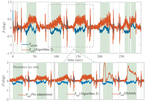
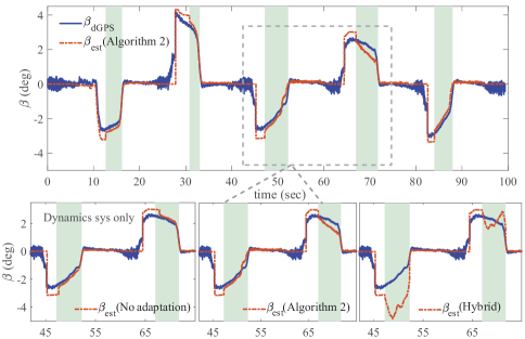
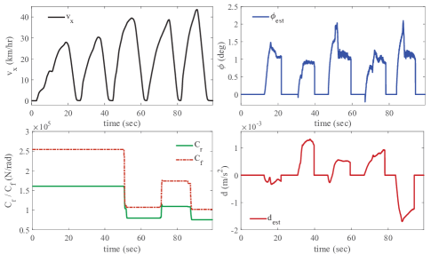
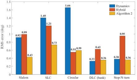
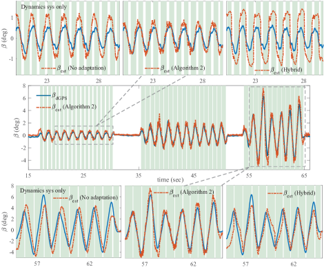
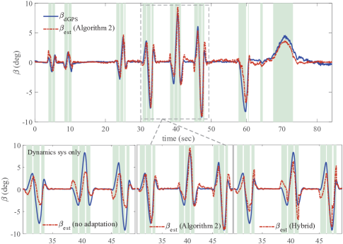
The experimental results are shown in Fig. 9-18 and the comparison of RMS error performances can be found in Fig. 8. As we can see, both the hybrid and dynamics observers exhibit a large RMS value under some driving situations. Algorithm 2 provides superior performances in all scenario tests.
Refer to caption
Figure 9: Comparison of the sideslip angle estimation for a slalom test.
Refer to caption
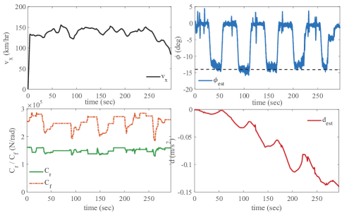
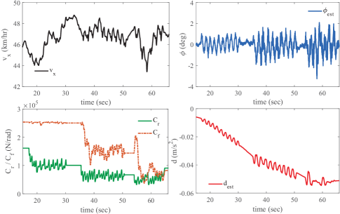
Figure 10: Slalom test results for Algorithm 2: longitudinal velocity; adapted cornering stiffnesses; estimated bank angle and sensor bias.

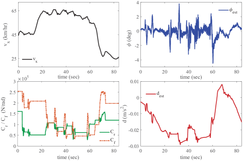
Starting from slalom, severe single lane changing and steady circular motion tests, we can see that Fig. 9, Fig. 11 and Fig. 13 demonstrate the effectiveness of the proposed estimator. For the dynamics model-based approach, it is obvious that there is a big disparity between the true and the estimated sideslip angle when the vehicle enters the nonlinear tire region. As expected, for the method switching between dynamics and kinematics models, we can see a discontinuous estimating during the transition. The longitudinal velocity, adapted tire cornering stiffnesses, estimated bank angle and sensor bias for all scenario tests are shown in Fig. 10, Fig. 12 and Fig. 14. The adapted cornering stiffnesses becomes smaller for a low friction road condition or entering the nonlinear tire region. Since the estimated bank angle is affected by the vehicle roll angle, we can conclude that all the estimated bank angle resulting within -4- 4 may be questionable. However, we still trust the estimation for large bank angles. Fig. 15 and Fig. 16 shows the experimental results of double lane change tests on a road with a large bank angle. The estimate performance of the switching algorithm is poor since the kinematics model is sensitive to the lateral acceleration measurement disturbance introduced from the bank angle. Fig. 16 confirms the ability of the proposed algorithm to estimating the bank angle, with the estimated value of the bank angle converging to the true value of 14. The adapted cornering stiffnesses remain unchanged because of the mild driving condition. Finally, we evaluate the performance of Algorithm 2 by conducting a stop-N-turn test for a varying low speed condition (Fig. 17 and Fig. 18). Again, the results are very promising.
Refer to caption
Figure 11: Comparison of the sideslip angle estimation for a severe single lane changing maneuver.
Refer to caption
Figure 12: Severe single lane changing test results for Algorithm 2: longitudinal velocity; adapted cornering stiffnesses; estimated bank angle and sensor bias.

In summary, the proposed algorithm stands out for its robustness in model error and measurement disturbance. It can be used for any driving situation with different road conditions. In addition, reliable estimates for bank angle and sensor bias are also available.

VII Conclusion

This paper developed a real-time algorithm for estimation of sideslip angle using inexpensive sensors normally available for electronic stability control (ESC) applications. The algorithm utilizes a kinematics observer to improve the estimation based on a vehicle dynamics model. It also provides estimates of road bank angles, lateral acceleration sensor bias and tire cornering stiffness. The algorithm performance is evaluated through several experimental tests and the results indicate that the algorithm provides a good estimate of the vehicle sideslip angle both in normal and extreme maneuvers with different road conditions.
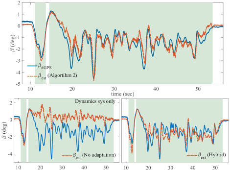
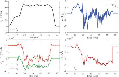
Refer to caption
Figure 13: Comparison of the sideslip angle estimation for a steady circular motion.
Refer to caption
Figure 14: Steady circular motion test results for Algorithm 2: longitudinal velocity; adapted cornering stiffnesses; estimated bank angle and sensor bias.
Refer to caption
Figure 15: Comparison of the sideslip angle estimation for double lane changing on a bank.
Refer to caption
Figure 16: On-bank double lane changing test results for Algorithm 2: longitudinal velocity; adapted cornering stiffnesses; estimated bank angle and sensor bias.
Refer to caption
Figure 17: Comparison of the sideslip angle estimation for a stop-N-turn motion.
Refer to caption
Figure 18: Stop-N-turn test results for Algorithm 2: longitudinal velocity; adapted cornering stiffnesses; estimated bank angle and sensor bias.

Appendix A Asymptotic Hyperstability and strictly positive real [33]

Definition 1.

The feedback system shown in Fig. 3 is asymptotically hyperstable if the state xksubscript𝑥𝑘x_{k} of the linear time invariant system converges to zero for k𝑘k\rightarrow\infty

Theorem A.1.

The feedback system shown in Fig. 3 is asymptotically hyperstable if and only if

  1. 1.

    the linear time invariant system is strictly positive real.

  2. 2.

    the nonlinear feedback block satisfies Popov inequality:

    γ>0,k=1k1wkTvkγ2k10formulae-sequence𝛾0formulae-sequencesuperscriptsubscript𝑘1subscript𝑘1subscriptsuperscript𝑤𝑇𝑘subscript𝑣𝑘superscript𝛾2for-allsubscript𝑘10\displaystyle\exists~{}\gamma>0,\quad\sum_{k=1}^{k_{1}}w^{T}_{k}v_{k}\geq-\gamma^{2}\quad\forall k_{1}\geq 0
  3. 3.

    the output signal, wksubscript𝑤𝑘w_{k}, of the nonlinear block is bounded.

Theorem A.2.

A single input single output discrete-time system, G(z)𝐺𝑧G(z), is strictly positive real if

  1. 1.

    the system does not possess any pole outside of or on the unit circle on z-plane.

  2. 2.

    |ω|<π,G(ejω)+G(ejω)>0formulae-sequencefor-all𝜔𝜋𝐺superscript𝑒𝑗𝜔𝐺superscript𝑒𝑗𝜔0\forall~{}|\omega|<\pi,~{}G(e^{-j\omega})+G(e^{j\omega})>0

Acknowledgment

The authors gratefully acknowledge the financial support received from the Hyundai Motor Company and the Hyundai-Kia Motors California Proving Ground for supporting this work. Thanks to Wanki Cho, Jinhwan Choi and Jongho Lee for the technical support.

References

  • [1] T. Pilutti, G. Ulsoy, and D. Hrovat, “Vehicle steering intervention through differential braking,” Journal of dynamic systems, measurement, and control, vol. 120, no. 3, pp. 314–321, 1998.
  • [2] H. E. Tseng, B. Ashrafi, D. Madau, T. A. Brown, and D. Recker, “The development of vehicle stability control at ford,” IEEE/ASME transactions on mechatronics, vol. 4, no. 3, pp. 223–234, 1999.
  • [3] M. Hara, S. Kamio, M. Takao, K. Sakita, and T. Abe, “Traction control system,” May 28 1991, uS Patent 5,018,595.
  • [4] R. Wilson-Jones, R. H. A. H. Tribe, and M. Appleyard, “Driver assistance system for a vehicle,” Jun. 9 1998, uS Patent 5,765,116.
  • [5] S. Lee and J.-B. Song, “Robust mobile robot localization using optical flow sensors and encoders,” in Robotics and Automation, 2004. Proceedings. ICRA’04. 2004 IEEE International Conference on, vol. 1.   IEEE, 2004, pp. 1039–1044.
  • [6] D. M. Bevly, J. Ryu, and J. C. Gerdes, “Integrating ins sensors with gps measurements for continuous estimation of vehicle sideslip, roll, and tire cornering stiffness,” IEEE Transactions on Intelligent Transportation Systems, vol. 7, no. 4, pp. 483–493, 2006.
  • [7] D. M. Bevly, J. C. Gerdes, C. Wilson, and G. Zhang, “The use of gps based velocity measurements for improved vehicle state estimation,” in American Control Conference, 2000. Proceedings of the 2000, vol. 4.   IEEE, 2000, pp. 2538–2542.
  • [8] D. Selmanaj, M. Corno, G. Panzani, and S. Savaresi, “Robust vehicle sideslip estimation based on kinematic considerations,” IFAC-PapersOnLine, vol. 50, no. 1, pp. 14 855–14 860, 2017.
  • [9] J. Farrelly and P. Wellstead, “Estimation of vehicle lateral velocity,” in Control Applications, 1996., Proceedings of the 1996 IEEE International Conference on.   IEEE, 1996, pp. 552–557.
  • [10] S. Strano and M. Terzo, “Constrained nonlinear filter for vehicle sideslip angle estimation with no a priori knowledge of tyre characteristics,” Control Engineering Practice, vol. 71, pp. 10–17, 2018.
  • [11] J. Dakhlallah, S. Glaser, S. Mammar, and Y. Sebsadji, “Tire-road forces estimation using extended kalman filter and sideslip angle evaluation,” in American Control Conference, 2008.   IEEE, 2008, pp. 4597–4602.
  • [12] Y. Aoki, T. Inoue, and Y. Hori, “Robust design of gain matrix of body slip angle observer for electric vehicles and its experimental demonstration,” in Advanced Motion Control, 2004. AMC’04. The 8th IEEE International Workshop on.   IEEE, 2004, pp. 41–45.
  • [13] L. Li, G. Jia, X. Ran, J. Song, and K. Wu, “A variable structure extended kalman filter for vehicle sideslip angle estimation on a low friction road,” Vehicle System Dynamics, vol. 52, no. 2, pp. 280–308, 2014.
  • [14] L. Shao, C. Jin, C. Lex, and A. Eichberger, “Nonlinear adaptive observer for side slip angle and road friction estimation,” in Decision and Control (CDC), 2016 IEEE 55th Conference on.   IEEE, 2016, pp. 6258–6265.
  • [15] S.-H. You, J.-O. Hahn, and H. Lee, “New adaptive approaches to real-time estimation of vehicle sideslip angle,” Control Engineering Practice, vol. 17, no. 12, pp. 1367–1379, 2009.
  • [16] C.-S. Liu and H. Peng, “A state and parameter identification sclieme for linearly parameterized systems,” 1998.
  • [17] H. F. Grip, L. Imsland, T. A. Johansen, J. C. Kalkkuhl, and A. Suissa, “Vehicle sideslip estimation,” IEEE control systems, vol. 29, no. 5, 2009.
  • [18] J. L. Coyte, B. Li, H. Du, W. Li, D. Stirling, and M. Ros, “Decision tree assisted ekf for vehicle slip angle estimation using inertial motion sensors,” in Neural Networks (IJCNN), 2014 International Joint Conference on.   IEEE, 2014, pp. 940–946.
  • [19] A. Y. U. H. Peng and H. Tseng, “Experimental verification of lateral speed estimation methods,” a a, vol. 1.
  • [20] B. Boada, M. Boada, and V. Diaz, “Vehicle sideslip angle measurement based on sensor data fusion using an integrated anfis and an unscented kalman filter algorithm,” Mechanical Systems and Signal Processing, vol. 72, pp. 832–845, 2016.
  • [21] C. M. Kang, S.-H. Lee, and C. C. Chung, “Vehicle lateral motion estimation with its dynamic and kinematic models based interacting multiple model filter,” in Decision and Control (CDC), 2016 IEEE 55th Conference on.   IEEE, 2016, pp. 2449–2454.
  • [22] B.-C. Chen and F.-C. Hsieh, “Sideslip angle estimation using extended kalman filter,” Vehicle System Dynamics, vol. 46, no. S1, pp. 353–364, 2008.
  • [23] D. Piyabongkarn, R. Rajamani, J. A. Grogg, and J. Y. Lew, “Development and experimental evaluation of a slip angle estimator for vehicle stability control,” IEEE Transactions on Control Systems Technology, vol. 17, no. 1, pp. 78–88, 2009.
  • [24] M. De Martino, F. Farroni, N. Pasquino, A. Sakhnevych, and F. Timpone, “Real-time estimation of the vehicle sideslip angle through regression based on principal component analysis and neural networks,” in Systems Engineering Symposium (ISSE), 2017 IEEE International.   IEEE, 2017, pp. 1–6.
  • [25] A. Y. Ungoren, H. Peng, and H. Tseng, “A study on lateral speed estimation methods,” International Journal of Vehicle Autonomous Systems, vol. 2, no. 1-2, pp. 126–144, 2004.
  • [26] R. Rajamani, Vehicle dynamics and control.   Springer Science & Business Media, 2011.
  • [27] R. Tibshirani, “Regression shrinkage and selection via the lasso,” Journal of the Royal Statistical Society, Series B, vol. 58, pp. 267–288, 1994.
  • [28] E. M. Eksioglu and A. K. Tanc, “Rls algorithm with convex regularization,” IEEE Signal Processing Letters, vol. 18, no. 8, pp. 470–473, 2011.
  • [29] I. D. Landau, “System identification and control design,” 1990.
  • [30] Y. Song and J. W. Grizzle, “The extended kalman filter as a local asymptotic observer for nonlinear discrete-time systems,” in American Control Conference, 1992.   IEEE, 1992, pp. 3365–3369.
  • [31] B. Anderson, “A simplified viewpoint of hyperstability,” IEEE Transactions on Automatic Control, vol. 13, no. 3, pp. 292–294, 1968.
  • [32] H. K. Khalil, “Noninear systems,” Prentice-Hall, New Jersey, vol. 2, no. 5, pp. 5–1, 1996.
  • [33] Y. Landau, “Adaptive control: the model reference approach, 1979,” Marcel Dekker, New York). Hac, A. Adaptive control of vehicle suspension. Veh. System Dynamics, vol. 16, pp. 74–77, 1987.
[Uncaptioned image] Yi-Wen Liao received the B.S. degree in mechanical engineering from National Taiwan University, Taipei, Taiwan, in 2010, and the M.S. degree in mechanical engineering from the University of Michigan, Ann Arbor, MI, USA, in 2012. She is currently working toward the Ph. D. degree in the Department of Mechanical Engineering at the Model Predictive Control Laboratory, University of California, Berkeley, headed by Prof. Francesco Borrelli. Her research interests include robust model predictive control, adaptive nonlinear control, vehicle dynamics, and their applications to autonomous driving systems.
[Uncaptioned image] Francesco Borrelli received the Laurea degree in computer science engineering from the University of Naples Federico II, Naples, Italy, in 1998, and the Ph.D. degree from ETH-Zurich, Zurich, Switzerland, in 2002. He is currently a Professor with the Department of Mechanical Engineering, University of California, Berkeley, CA, USA. He is the author of more than 100 publications in the field of predictive control and author of the book Constrained Optimal Control of Linear and Hybrid Systems (Springer-Verlag). His research interests include constrained optimal control, model predictive control and its application to advanced automotive control and energy efficient building operation. Dr. Borrelli received the 2009 National Science Foundation CAREER Award and the 2012 IEEE Control System Technology Award. In 2008, he became the Chair of the IEEE Technical Committee on Automotive Control.