A Bound on Chaos from Stability

Abstract

We explore the quantum chaos of the coadjoint orbit action of diffeomorphism group of $S^{1}$. We study quantum fluctuation around a saddle point to evaluate the soft mode contribution to the out-of-time-ordered correlator. We show that the stability condition of the semi-classical analysis of the coadjoint orbit found in Witten:1987ty leads to the upper bound on the Lyapunov exponent which is identical to the bound on chaos proven in Maldacena:2015waa . The bound is saturated by the coadjoint orbit Diff$(S^{1})/SL(2)$ while the other stable orbit Diff$(S^{1})/U(1)$ where the $SL(2,\mathbb{R})$ is broken to $U(1)$ has non-maximal Lyapunov exponent.

1 Introduction

Chaos is a ubiquitous phenomenon observed in the nature. One way to diagnose the chaos is the butterfly effect which is known as the sensitivity of the system on the initial condition. In quantum system, this can be quantified by a thermal expectation value of the square of the commutator of two operators $V(t)$ and $W(0)$. This measures the sensitivity of the operator $V(t)$ at time $t$ on the initial perturbation $W(0)$ at time $t=0$ Shenker:2013pqa ; Shenker:2014cwa . In chaotic system, this is expected to grow exponentially in time $t$. This exponential growth comes from the out-of-time-ordered correlator (OTOC)

$$\langle V(t)W(0)V(t)W(0)\rangle_{\beta}\,\equiv\,\mbox{Tr\,}\big{[}e^{-{\beta H\over 4}}\,V(t)\,e^{-{\beta H\over 4}}\,W(0)\,e^{-{\beta H\over 4}}\,V(t)\,e^{-{\beta H\over 4}}\,W(0)\big{]}\ ,$$ (2)

which is one of terms in the expansion of the square of the commutator. Here, $\beta=T^{-1}$ is the inverse of the temperature. We normalize the OTOC by the leading disconnected diagrams $\langle V(t)V(t)\rangle_{\beta}\langle W(0)W(0)\rangle_{\beta}$ which is independent of time by time translational symmetry. The normalized OTOC of the chaotic system behaves as follow Shenker:2013pqa ; Shenker:2014cwa .

$$\mathcal{F}(t)\,\equiv\,{\langle V(t)W(0)V(t)W(0)\rangle_{\beta}\over\langle V(t)V(t)\rangle_{\beta}\langle W(0)W(0)\rangle_{\beta}}\,=\,1-\varepsilon e^{\lambda_{L}t}\ ,$$ (3)

where $\varepsilon$ is inversely proportional to the logarithm of the entropy $S$. For example, it is proportional to ${1\over N}$ and ${1\over N^{2}}$ in large $N$ vector and matrix models, respectively, and accordingly it is proportional to the Newton constant $G$ in the holographic dual gravity. This bound is shown to be saturated by CFTs dual to Einstein gravity Shenker:2013pqa . In early time, the OTOC is almost constant. As time passes, one can observe the exponential growth in the OTOC , and its growth rate $\lambda_{L}$ is called Lyapunov exponent.

Maldacena:2015waa proved that the Lyapunov exponent of any QFT with basic constraints (e.g., unitarity and causality) is bounded:

$$\lambda_{L}\leqq{2\pi\over\beta}\ .$$ (4)

This bound implies that there possibly exist maximally chaotic systems. Indeed, it was shown that the SYK model Sachdev:1992fk ; kitaevfirsttalk ; KitaevTalks ; Polchinski:2016xgd ; Jevicki:2016bwu ; Maldacena:2016hyu ; Jevicki:2016ito , the tensor model Gurau:2010ba ; Carrozza:2015adg ; Witten:2016iux ; Gurau:2016lzk ; Klebanov:2016xxf , the 2D dilaton gravity on nearly-AdS₂ Maldacena:2016upp and string worldsheet theories deBoer:2017xdk are maximally chaotic. By recovering all dimensionful parameters, the maximum value of Lyapunov exponent becomes ${2\pi k_{B}\over\hbar\beta}$, and it diverges in the classical limit. For this reason, (4) can be viewed as the bound on quantum chaos.

In this paper, we will show that the bound on quantum chaos can also be derived from the stability of semi-classical analysis of Schwarzian theory. Unlike Maldacena:2015waa of which the proof of the bound on chaos is valid for any QFT with unitarity and causality, our discussion is restricted to the Schwarzian theory and is not as general as that of Maldacena:2015waa . Nevertheless, our analysis provides a very simple physical argument for the bound, which would reveal the underlying physical meaning of the bound on chaos.

2 Schwarzian Theory and Coadjoint Orbit Action

In SYK-like model and 2D dilaton gravity, the reparametrization symmetry along the thermal circle is broken to $SL(2,\mathbb{R})$, which leads to the pseudo-Goldstone boson described by the Schwarzian low energy effective action:

$$S=\int_{0}^{2\pi}d\tau\;\left(-{c\over 12}\mbox{Sch}\!\left[\phi(\tau),\tau\right]-{c\over 24}[\phi^{\prime}(\tau)]^{2}\right)\ .$$ (5)

Here, $\phi(\tau)\in$Diff$(S^{1})/SL(2)$ is a diffeomorphism of the circle modulo $SL(2,\mathbb{R})$.

Now, let us consider the case where the reparametrization symmetry is broken to $U(1)\subset SL(2,\mathbb{R})$. For example, such a pattern of symmetry breaking has been observed in the generalized SYK-like models in Ferrari:2019ogc and the 2D dilaton gravity with defects in Anninos:2018svg ; Mertens:2019tcm . For their low energy effective action, one can include not only Schwarzian derivatives but also any possible terms which vanish under the corresponding $U(1)$ mode. Hence, the simplest effective action can be written as

$$S= \int d\tau\;\left(-{c\over 12}\mbox{Sch}\!\left[\phi(\tau),\tau\right]+b_{0}[\phi^{\prime}(\tau)]^{2}\right)\ ,$$ (6)

where $b_{0}$ is a constant. This is nothing but the time-translation generator $L_{0}$ of a coadjoint orbit $\phi(\tau)\in\text{Diff}/H$ where $H$ is the stabilizer subgroup Witten:1987ty ; Stanford:2017thb .

We will briefly review the coadjoint representation and its time-translation generator Witten:1987ty ; Alekseev:1988ce ; Rai:1989js ; Stanford:2017thb ; Cotler:2018zff . Let us consider the element $(v(\tau),a)$ of the central extension of the Diff$(S^{1})$which corresponds to Virasoro group. Here, $a$ is the central charge. The dual vector $(b(\tau),c)$ of the central extension of Diff$(S^{1})$ can be induced via the inner product defined by

$$\langle(b(\tau),c),(v(\tau),a)\rangle\equiv\int_{0}^{2\pi}{d\tau\over 2\pi}b(\tau)v(\tau)+ca\ .$$ (7)

The adjoint representation of $\phi\in$Diff$(S^{1})$ on the vector $(v(\tau),a)$ is defined by Witten:1987ty ; Alekseev:1988ce ; Rai:1989js

$$\text{Ad}_{\phi^{-1}}(v(\tau),a)\,=\,\left({v(\phi(\tau))\over\phi^{\prime}(\tau)},a+{1\over 12}\int{d\tau\over 2\pi}{v(\phi(\tau))\over\phi^{\prime}(\tau)}\mbox{Sch}\![\phi(\tau),\tau]\right)\ .$$ (8)

Via the inner product in (7), the adjoint representation (8) induces the coadjoint representation on the dual vector $(b(\tau),c)$. In particular, we are interested in a coadjoint orbit of a constant dual vector $(b_{0},c)$ Witten:1987ty ; Stanford:2017thb :

$$\text{Ad}^{\ast}_{\phi^{-1}}[(b_{0},c)]=\left(\big{[}\phi^{\prime}(\tau)\big{]}^{2}b_{0}-{c\over 12}\mbox{Sch}\!\left[\phi(\tau),\tau\right],c\right)\ .$$ (9)

Depending on the constant value of $b_{0}$, the stabilizer of the coadjoint representation $\text{Ad}^{\ast}_{\phi^{-1}}$ is different. For example, for $b_{0}\neq-{cn^{2}\over 24}$ ($n\in\mathbb{N}$), the coadjoint representation $\text{Ad}^{\ast}_{\phi^{-1}}$ is invariant under the $U(1)$ transformation of $\phi(\tau)\;\;\rightarrow\;\;\phi(\tau)+a$ ($a$: constant). On the other hand, the stabilizer subgroup is $SL(2,\mathbb{R})$ for $b_{0}=-{c\over 24}$. Hence, the coadjoint orbit is isomorphic to Diff$(S^{1})/U(1)$ or Diff$(S^{1})/SL(2)$ for $b_{0}\neq-{cn^{2}\over 24}$ or $b_{0}=-{c\over 24}$, respectively.

The Hamiltonian corresponding to the Virasoro generator $L_{0}=i{\partial\over\partial\tau}$ can be obtained from the inner product of $\text{Ad}^{\ast}_{\phi^{-1}}(b(\tau))$ and a constant vector Witten:1987ty . This leads to the Schwarzian action in (6).

In large $c>0$, one can perform the semi-classical analysis of the Schwarzian action in (6) by studying the quantum fluctuation around the identity diffeomorphism $\phi(\tau)=\tau$. The quadratic action in the large $c$ expansion of the action reads

$$S^{(2)}\,\sim\,\sum_{n}n^{2}\left(n^{2}+{24\over c}b_{0}\right)\epsilon_{-n}\epsilon_{n}\ .$$ (10)

Therefore the fluctuation $\epsilon_{n}$ at the quadratic level (in particular, $\epsilon_{1}$) is stable if

$$b_{0}\geqq-{c\over 24}\ .$$ (11)

Note that this bound is saturated by Diff$(S^{1})/SL(2)$. Otherwise, the stable coadjoint orbit corresponds to Diff$(S^{1})/U(1)$ Witten:1987ty . This bound comes from the zero $n=\sqrt{-{24\over c}b_{0}}$ of the quadratic action which also play a crucial role in the Lyapunov exponent of OTOC.

3 Out-of-time-ordered Correlators

Now, we will evaluate the contribution of the Schwarzian mode to OTOC. As in the SYK-like model or the dilaton gravity on nearly-AdS₂, we assume that the contribution of the Schwarzian mode dominates the four point OTOC. We first evaluate the contribution of the Schwarzian mode to the Euclidean four point function. Then, we will take analytic continuation to a real-time OTOC.

3.1 Propagator of Soft Mode

In large $c$, we expand the diffeomorphism $\phi(\tau)$ around the identity $\phi(\tau)=\tau$:

$$\phi(\tau)=\tau+{1\over\sqrt{c}}\sum_{|n|\geqq n_{0}}\epsilon_{n}e^{-in\tau}\ .$$ (12)

Here, we define $n_{0}=1$ or $n_{0}=2$ for the case of Diff$(S^{1})/U(1)$ or Diff$(S^{1})/SL(2)$, respectively. Note that $|n|<n_{0}$ corresponds to the stabilizer subgroup of the coadjoint representation. The soft mode expansion in (12) gives the quadratic action of (6):

$$S^{(2)}={\pi\over 12}\sum_{|n|>n_{0}}n^{2}\left(n^{2}+{24\over c}b_{0}\right)\epsilon_{-n}\epsilon_{n}\ .$$ (13)

From the quadratic action, one can easily read off the propagator of the soft mode $\epsilon_{n}$

$$\langle\epsilon_{-n}\epsilon_{n}\rangle={{6\over\pi}\over n^{2}\left(n^{2}+{24\over c}b_{0}\right)}\qquad\mbox{for}\quad|n|>n_{0}\ .$$ (14)

3.2 Dressed Bi-local Field

In order to evaluate OTOC, one need a “matter” field and its four point function. In SYK model, the four point function of the fundamental fermion $\chi^{i}(\tau)$ ($i=1,2,\cdots,N)$ can be evaluated as a two point function of bi-local field $\Psi(\tau_{1},\tau_{2})\equiv{1\over N}\sum_{i=1}^{N}\chi^{i}(\tau_{1})\chi^{i}(\tau_{2})$ Jevicki:2016bwu ; Maldacena:2016hyu . Also, for the case of the nearly-AdS₂, Maldacena:2016upp evaluated the OTOC by studying the two point function of bi-locals coming from a scalar field in the nearly-AdS₂.

One essential ingredient of the OTOC calculation is the infinitesimal transformation of the two point function of the matter field under the symmetry related to the soft mode Maldacena:2016hyu ; Yoon:2017nig ; Narayan:2019ove ; Jahnke:2019gxr . For example, one need to calculate the reparametrization transformation of the two point function in SYK model or its holographic dual near-AdS₂. Such a transformation gives us the coupling between matter and soft mode in the soft mode channel of OTOC. In general, soft modes require the transformation of the two point function of matters under the corresponding symmetry. However, in the field theory such a transformation is not always known unlike reparametrization symmetry. For instance, the transformation of the two point function under the $\mathcal{W}_{N}$ symmetry, which is involved with the higher spin soft modes, is still not fully understood in the field theory. On the other hand, such a transformation can easily be evaluated holographically by a (boundary-to-boundary) Wilson line of the gauge field in $SL(2)$ BF theory for AdS₂ Blommaert:2018oro ; Lam:2018pvp ; Blommaert:2018iqz ; Mertens:2019tcm ; Iliesiu:2019xuh or Chern-Simons gravity for AdS₃ Jahnke:2019gxr ; Narayan:2019ove . The boundary-to-boundary Wilson line in the AdS₂ bulk can reproduce the two point function deBoer:2013vca ; Ammon:2013hba ; Castro:2018srf ; Narayan:2019ove of its holographic dual field theory, and it is gauge invariant except for the end points. In particular, the Wilson line out of a general gauge field $A$ of $SL(2)$ BF theory or Chern-Simons gravity can be understood as gravitationally dressed two point function Jahnke:2019gxr ; Narayan:2019ove . For more general BF or Chern-Simons gravity, one can consider a small fluctuation around a fixed background gauge field corresponding to the AdS background, which leads to the expansion of the gravitationally dressed Wilson line with respect to a small fluctuation (See Jahnke:2019gxr ; Narayan:2019ove for the details). In the small fluctuation expansion, the leading term reproduces the boundary-to-boundary two point function in the fixed AdS background in the bulk theory which corresponds to the two point function in the dual field theory. In addition, the first correction term exactly gives the infinitesimal transformation of the two point function of the dual field theory under symmetry generated by the boundary soft modes. Note that the small fluctuation corresponds to the small fluctuation corresponds to soft mode living on the boundary of AdS₂. For the case of $SL(2)$ BF gravity, it is governed by Schwarzian boundary action for the boundary graviton Maldacena:2016upp ; Cvetic:2016eiv ; Mandal:2017thl ; Grumiller:2017qao ; Castro:2018ffi ; Cotler:2018zff ; Jahnke:2019gxr ; Narayan:2019ove . This provides the physical intuition why we need such a transformation for OTOC calculations.

In order for the contribution of the soft mode $\epsilon_{n}$ to the four point function, we consider the two point function of the (boundary-to-boundary) Wilson lines of a gauge field $A$ which can be understood as the bi-local field dressed by the soft mode Maldacena:2016upp ; Jahnke:2019gxr ; Narayan:2019ove .

$$\langle\Phi^{\text{\tiny dressed}}(\tau_{1},\tau_{2})\Phi^{\text{\tiny dressed}}(\tau_{3},\tau_{4})\rangle\ .$$ (15)

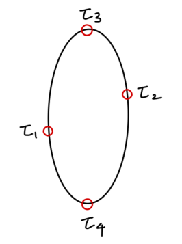
(a) Thermal Circle

$\xRightarrow[\text{continuation}]{\text{analytic}}$

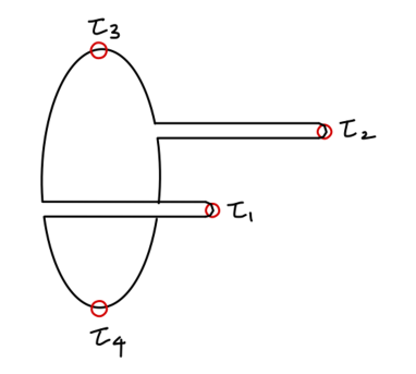
(b) Real-time OTO

Figure 1: We evaluate the Euclidean four point function for the configuration in (16). Then, we analytic-continue it to real-time OTOC by (27).

For the real-time OTOC, we first evaluate the Euclidean correlator with the configuration along the thermal circle

$$(\tau_{1},\tau_{2},\tau_{3},\tau_{4})=(\chi-{\pi\over 2},\chi+{\pi\over 2},0,\pi)\ ,$$ (16)

where $\chi\in(-\pi/2,\pi/2)$ (See Figure 1a) Maldacena:2016hyu ; Maldacena:2016upp . Then, later we will perform the analytic continuation of the Euclidean time $\chi$ to a real time $t$.

In large $c$, one can expand the dressed bi-local field with respect to the soft mode $\epsilon_{n}$:

$${\Phi^{\text{\tiny dressed}}(\tau_{1},\tau_{2})\over\Phi_{cl}(\tau_{1},\tau_{2})}\,=\,1+\sum_{|n|\geqq n_{0}}{\epsilon_{n}\over\sqrt{c}}{\delta_{\epsilon_{n}}\Phi^{\text{\tiny dressed}}(\tau_{1},\tau_{2})\over\Phi_{cl}(\tau_{1},\tau_{2})}+\mathcal{O}(c^{-1})\ ,$$ (17)

where $\Phi_{cl}(\tau_{1},\tau_{2})$ is the leading term of the soft mode expansion of the dressed bi-local, and it corresponds to the two point function in the constant background. e.g., $\Phi_{cl}(\tau_{1},\tau_{2})\!\sim\!{1\over|\sin{\pi\tau_{12}\over\beta}|^{2h}}$. Recall that both Diff$(S^{1})/SL(2)$ and Diff$(S^{1})/U(1)$ has $U(1)$ time translational symmetry. From the (center of) time translational symmetry, one can write the first order soft mode expansion in (17) as follow.

$${\delta_{\epsilon_{n}}\Phi^{\text{\tiny dressed}}(\tau_{1},\tau_{2})\over\Phi_{cl}(\tau_{1},\tau_{2})}=e^{-in\chi}f_{n}(\sigma)\ ,$$ (18)

where we define the center of time and the relative time by

$$\chi\equiv{1\over 2}(\tau_{1}+\tau_{2})\quad,\quad\sigma\equiv{1\over 2}(\tau_{1}-\tau_{2})\ ,$$ (19)

respectively. Also, note that $\delta_{\epsilon_{n}}\Phi^{\text{\tiny dressed}}(\tau_{1},\tau_{2})$ can be obtained from the infinitesimal conformal transformation of two point function because the soft mode generates the conformal transformation.

The soft mode expansion of the dressed bi-locals gives the $1/c$ contribution of the Schwarzian soft mode to the Euclidean four point function, or equivalently two point function of the dressed bi-locals, in (15). I.e.,

$$\mathcal{F}(\chi)\equiv{\langle\Phi^{\text{\tiny dressed}}(\chi-\pi/2,\chi+\pi/2)\Phi^{\text{\tiny dressed}}(0,\pi)\rangle\over\Phi_{cl}(\chi-\pi/2,\chi+\pi/2)\Phi_{cl}(0,\pi)}$$ (20)

$$\,=\, 1+{1\over c}\sum_{|n|\geqq n_{0}}\langle\epsilon_{-n}\epsilon_{n}\rangle e^{in\chi}e^{-{n\pi i\over 2}}f_{-n}(-{\pi\over 2})f_{n}(-{\pi\over 2})\ .$$ (21)

Here, we used the configuration in (16). We will calculate the soft mode contribution for Diff$(S^{1})/SL(2)$ case and Diff$(S^{1})/U(1)$ case, separately.

3.2 Diff$(S^{1})/SL(2)$ case. For the case of Diff$(S^{1})/SL(2)$, the soft mode eigenfunction $f(\sigma)$ is found to be Maldacena:2016hyu

$$f_{n}(\sigma)\,=\,-2ih\left[n\cos n\sigma-{\sin n\sigma\over\tan\sigma}\right]\ ,$$ (22)

where $h$ is the conformal dimension of the matter field. Note that the $SL(2,\mathbb{R})$ invariance of the bi-local fields (e.g., boundary-to-boundary Wilson line or conformal two point function) leads to

$$f_{n}(\sigma)\,=\,0\hskip 22.76219pt\mbox{for}\quad n=0,\pm 1\ .$$ (23)

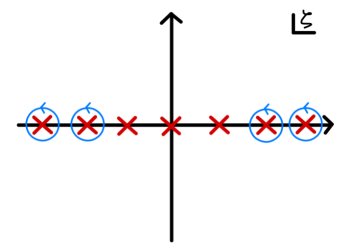
(a)

$\xRightarrow[\text{contour}]{\text{deform}}$

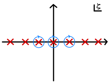
(b)

Figure 2: The soft mode contribution can be written as a contour integral along a collection of small counterclockwise circles centered at $\zeta\in\mathbb{Z}/\{-1,0,1\}$. By deforming the contour, it can be expressed as the residue at $\zeta=-1,0,1$.

Together with the propagator of soft mode in (14), the soft mode expansion in (21) can be written as a contour integral as follow Narayan:2017qtw ; Yoon:2017nig ; Narayan:2017hvh ; Jahnke:2019gxr ; Narayan:2019ove .

$$\mathcal{F}(\chi)=1+{24h^{2}\over\pi c}{1\over 2\pi i}\oint_{\mathcal{C}}d\zeta\;{{\pi\over 2}\over\sin{\pi\zeta\over 2}}{e^{i\zeta\chi}\over\zeta^{2}-1}\ ,$$ (24)

where the contour $\mathcal{C}$ is a collection of small counterclockwise circles around $\zeta=n$ ($n\in\mathbb{Z}/\{-1,0,1\}$). See Figure 2a. Then, by deforming the contour, one can change it into a sum of residues at $\zeta=-1,0,1$ (See Figure 2b) Maldacena:2016hyu ; Maldacena:2016upp ; Sarosi:2017ykf ; Jahnke:2019gxr ; Narayan:2019ove :

$$\mathcal{F}(\chi)\,=\, 1-{24h^{2}\over\pi c}\sum_{n=0,\pm 1}\mathop{Res}\limits_{\zeta=n}\;{{\pi\over 2}\over\sin{\pi\zeta\over 2}}{e^{i\zeta\chi}\over\zeta^{2}-1}$$ (25)

$$\,=\, 1+{24h^{2}\over\pi c}\left(1-{\pi\over 2}\cos\chi\right)\ .$$ (26)

For the real-time OTOC, we perform the analytic continuation of the Euclidean time $\chi$ to real time $t$ (See Figure 1b). i.e.,

$$\chi\quad\longrightarrow\quad-{2\pi i\over\beta}t\ .$$ (27)

The analytic continuation gives the exponential growth with the maximal Lyapunov exponent $\lambda_{L}={2\pi\over\beta}$ Maldacena:2016hyu ; Maldacena:2016upp ; Narayan:2017qtw ; Yoon:2017nig ; Narayan:2017hvh ; Jahnke:2019gxr .

$$\mathcal{F}(t)\,=\,1-{6h^{2}\over c}e^{{2\pi\over\beta}t}+\cdots\ ,$$ (28)

where we omit the term does not grow exponentially in time at $\mathcal{O}(c^{-1})$ order.

3.3 Diff$(S^{1})/U(1)$ case

We repeat a similar calculation for the Diff$(S^{1})/U(1)$ case where $SL(2,\mathbb{R})$ is broken to $U(1)$. In this case, we also assume a matter field coupled to Diff$(S^{1})/U(1)$. And, its boundary-to-boundary two point function has $U(1)$ invariance. The infinitesimal transformation of the boundary-to-boundary correlation function will give the soft mode eigenfunction $f_{n}(\sigma)$. The form of the function $f_{n}(\sigma)$ in (18) might depend on the details of model. Nevertheless, the evaluation of the Lyapunov exponent can be independent of the form of the function $f_{n}(\sigma)$ because the calculation mainly uses the center of time translational symmetry and the structure of poles. In general, the contribution of the soft mode in (21) now includes $n=\pm 1$ terms because they do not belong to the stabilizer subgroup for the case of Diff$(S^{1})/U(1)$. Moreover, it might be possible that $f_{n}(-{\pi\over 2})=0$ for odd $n$ as in Diff$(S^{1})/SL(2)$. However, one can repeat the same calculation and it does not change the conclusion.

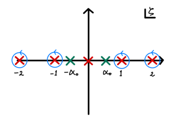
(a)

$\xRightarrow[\text{contour}]{\text{deform}}$

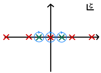
(b)

Figure 3: The soft mode contribution can be written as a contour integral along a collection of small counterclockwise circles centered at $\zeta\in\mathbb{Z}/\{0\}$. By deforming the contour, it can be expressed as the residue at $\zeta=0$ and $\pm\alpha_{0}\equiv\pm\sqrt{-{24\over c}b_{0}}$.

As in the Diff$(S^{1})/U(1)$ case, we express the soft mode contribution as a contour integral

$$\mathcal{F}(\chi)=1-{6\over\pi c}\oint_{\mathcal{C}}d\zeta{e^{i\zeta\chi}e^{-{i\pi\zeta\over 2}}\over e^{-2\pi i\zeta}-1}{f_{-\zeta}(-{\pi\over 2})f_{\zeta}(-{\pi\over 2})\over\zeta^{2}\left(\zeta^{2}+{24\over c}b_{0}\right)}\ ,$$ (29)

where $\mathcal{C}$ is a collection of small counterclockwise circles around $\zeta\in\mathbb{Z}/\{0\}$. See Figure 3a. Then, we will deform the contour to pick up the rest of the poles. For this, we need further assumptions on $f_{n}(-{\pi\over 2})$ that the integrand in (29) does not blow up at infinity, at least, for $\chi\in(-\delta,\delta)$ with a small positive constant $\delta$. Moreover, we assume that $f_{\pm\zeta}(-{\pi\over 2})$ have neither pole in the $\zeta$ plane nor zero at $\zeta=\pm\sqrt{-{24\over c}b_{0}}$. Then, the deformation of the contour gives (See Figure 3b)

$$\mathcal{F}(\chi)\,=\,1+{12i\over c}\sum_{n\in\mathcal{P}}\mathop{Res}\limits_{\zeta=n}{e^{i\zeta\chi}e^{-{i\pi\zeta\over 2}}\over e^{-2\pi i\zeta}-1}{f_{-\zeta}(-{\pi\over 2})f_{\zeta}(-{\pi\over 2})\over\zeta^{2}\left(\zeta^{2}+{24\over c}b_{0}\right)}\ ,$$ (30)

where we defined $\mathcal{P}\equiv\{0,\pm\sqrt{-{24\over c}b_{0}}\}$. Note that the pole at $\zeta=0$ would be simple pole because the time translational invariance of bi-locals imposes $f_{0}(\sigma)=0$. Even if $f_{0}(\sigma)\neq 0$, the pole at $\zeta=0$ does not change the Lyapunov exponent since it gives at most polynomial growth in time at $\mathcal{O}(c^{-1})$ order. Therefore, we have

$$\mathcal{F}(\chi)\,=\, 1-{6\over c}\cos\alpha_{0}(\chi+{\pi\over 2}){f_{-\alpha_{0}}(-{\pi\over 2})f_{\alpha_{0}}(-{\pi\over 2})\over\alpha_{0}^{3}\sin\pi\alpha_{0}}+\cdots\ ,$$ (31)

where we define $\alpha_{0}\equiv\sqrt{-{24\over c}b_{0}}$ for simplicity. Here, the ellipsis represents the contribution of the pole at $\zeta=0$ which does not grow exponentially after analytic continuation. By the analytic continuation (27) of (31) from Euclidean time to Lorentzian one (See Figure 1b), the OTOC for Diff$(S^{1})/U(1)$ is found to be

$$\mathcal{F}(t)\,=\,1-{3\over c}e^{{2\pi\alpha_{0}\over\beta}t}e^{\pi i\alpha_{0}\over 2}{f_{-\alpha_{0}}(-{\pi\over 2})f_{\alpha_{0}}(-{\pi\over 2})\over\alpha_{0}^{3}\sin\pi\alpha_{0}}+\cdots\ .$$ (32)

And, the Lyapunov exponent can easily be read off

$$\lambda_{L}\,=\,{2\pi\over\beta}\alpha_{0}\,=\,\sqrt{-{24\over c}b_{0}}\ .$$ (33)

For $b_{0}<0$, the bound on $b_{0}$ in (11) for stability of the coadjoint orbit Witten:1987ty in large $c$ leads to

$$\lambda_{L}\,=\,{2\pi\over\beta}\sqrt{{24\over c}|b_{0}|}<{2\pi\over\beta}\ ,$$ (34)

which corresponds to the bound on chaos proven in Maldacena:2015waa . For $b_{0}\geqq 0$, it is easy to see that the Lyapunov exponent is zero i.e., $\lambda_{L}=0$.

4 Conclusion

In this work, we have evaluated the Schwarzian soft mode contribution to the OTOC for the case of Diff$(S^{1})/SL(2)$ and Diff$(S^{1})/U(1)$. We have showed that the stability of the coadjoint orbit found in Witten:1987ty leads to the bound of chaos proven in Maldacena:2015waa . While this bound is saturated by Diff$(S^{1})/SL(2)$, the coadjoint orbit Diff$(S^{1})/U(1)$ where the $SL(2,\mathbb{R})$ is broken to $U(1)$ is not maximally chaotic. i.e., $\lambda_{L}<2\pi/\beta$.

The decrease of the Lyapunov exponent has been observed in the generalized SYK-like models exhibiting the transition from chaotic phase to non-chaotic phase (or, from non-Fermi liquid phase to Fermi liquid phase) Banerjee:2016ncu ; Garcia-Garcia:2017bkg ; Nosaka:2018iat ; Ferrari:2019ogc . The underlying mechanism for the decreased Lyapunov exponent in those models is the broken $SL(2,\mathbb{R})$ symmetry to $U(1)$ Ferrari:2019ogc . Furthermore, Anninos:2018svg ; Mertens:2019tcm studied the 2D dilaton gravity with defects where the $SL(2,\mathbb{R})$ isometry of AdS₂ background is broken to $U(1)$ due to the defect. This isometry of the background is responsible for the redundant description of the boundary modes, and it should be gauged. Therefore, the effective action for this case will be related to Diff$(S^{1})/U(1)$ rather than Diff$(S^{1})/SL(2)$. And one can also expect that the Lyapunov exponent does not saturate the bound (if the Schwarzian soft mode contribution dominates OTOC). In addition, this broken $SL(2,\mathbb{R})$ symmetry would essentially be responsible for the phase transition of the coupled SYK-like models dual to the traversable wormhole Maldacena:2018lmt ; Garcia-Garcia:2019poj ; Kim:2019upg where the phase transition is triggered by a similar (non-local) quadratic interactions.

In general, if the $SL(2,\mathbb{R})$ of a saddle point is broken to $U(1)$, all possible terms which vanish under $U(1)$ mode can appear in the effective action. For example, the simplest effective action can be written as

$$S_{\text{\tiny eff}}\,=\,-\kappa_{1}c\mbox{Sch}\!\left[\tan\left({\phi(\tau)\over 2}\right),\tau\right]+\kappa_{2}[\partial_{\tau}\phi(\tau)]^{2}\ ,$$ (35)

where $\kappa_{1}$ and $\kappa_{2}$ are constants to be determined. In large $c$, the stability of the semi-classical analysis, or equivalently, the chaos bound requires

$$\kappa_{2}\,\geqq\,0\ .$$ (36)

From the Lyapunov exponent in (33) together with stability bound in (11), one can also conclude that the instability of the coadjoint orbit action could lead to the violation of the bound on chaos. i.e., $\lambda_{L}>2\pi/\beta$. An analogous phenomenon has been observed in the higher spin gravity Perlmutter:2016pkf ; Narayan:2019ove and the Fishnet model deMelloKoch:2019ywq . The $SL(N)$ Chern-Simons higher spin gravity has finite numbers of higher spin fields (spin $s=2,3,\cdots,N$), and it is non-unitary. The Lyapunov exponent is found to be ${2\pi\over\beta}(N-1)$ which violates the bound on chaos for $N>2$. Moreover, the mass deformation of the Fishnet model destroys the integrability, but the Feynman diagrams are still simple. In this case, deMelloKoch:2019ywq showed that the Lyapunov exponent can exceed $2\pi/\beta$ in the large ’tHooft limit, which the non-unitarity of the Fishnet model is also responsible for.

It is interesting to explore the role of the stability in the context of “pole skipping” phenomenon Grozdanov:2017ajz ; Haehl:2018izb ; Blake:2018leo ; Grozdanov:2018kkt ; Grozdanov:2019uhi . The pole-skipping, which is universal in two-dimensional CFT, can determine the Lyapunov exponent Grozdanov:2017ajz ; Haehl:2018izb ; Blake:2018leo ; Grozdanov:2018kkt ; Grozdanov:2019uhi . Therefore, one might be able to find a connection between the (in)stability of hydrodynamics and the bound on chaos via the pole-skipping. Furthermore, this might suggest a universal framework to understand how the (in)stability of hydrodynamical effective action leads to the bound on chaos in higher dimensional CFT.

- (1) E. Witten, Coadjoint Orbits of the Virasoro Group, Commun. Math. Phys. 114 (1988) 1.
- (2) J. Maldacena, S. H. Shenker, and D. Stanford, A bound on chaos, JHEP 08 (2016) 106, [arXiv:1503.01409].
- (3) S. H. Shenker and D. Stanford, Black holes and the butterfly effect, JHEP 03 (2014) 067, [arXiv:1306.0622].
- (4) S. H. Shenker and D. Stanford, Stringy effects in scrambling, JHEP 05 (2015) 132, [arXiv:1412.6087].
- (5) K. Hashimoto, K. Murata, and R. Yoshii, Out-of-time-order correlators in quantum mechanics, JHEP 10 (2017) 138, [arXiv:1703.09435].
- (6) S. Sachdev and J. Ye, Gapless spin fluid ground state in a random, quantum Heisenberg magnet, Phys. Rev. Lett. 70 (1993) 3339, [cond-mat/9212030].
- (7) A. Kitaev, Hidden correlations in the Hawking radiation and thermal noise, http://online.kitp.ucsb.edu/online/joint98/kitaev/, KITP seminar, Feb. 12, (2015).
- (8) A. Kitaev, A simple model of quantum holography, http://online.kitp.ucsb.edu/online/entangled15/kitaev/, http://online.kitp.ucsb.edu/online/entangled15/kitaev2/, Talks at KITP, April 7, 2015 and May 27, (2015).
- (9) J. Polchinski and V. Rosenhaus, The Spectrum in the Sachdev-Ye-Kitaev Model, JHEP 04 (2016) 001, [arXiv:1601.06768].
- (10) A. Jevicki, K. Suzuki, and J. Yoon, Bi-Local Holography in the SYK Model, JHEP 07 (2016) 007, [arXiv:1603.06246].
- (11) J. Maldacena and D. Stanford, Remarks on the Sachdev-Ye-Kitaev model, Phys. Rev. D 94 (2016), no. 10 106002, [arXiv:1604.07818].
- (12) A. Jevicki and K. Suzuki, Bi-Local Holography in the SYK Model: Perturbations, JHEP 11 (2016) 046, [arXiv:1608.07567].
- (13) R. Gurau, The 1/N expansion of colored tensor models, Annales Henri Poincare 12 (2011) 829–847, [arXiv:1011.2726].
- (14) S. Carrozza and A. Tanasa, Random Tensor Models, Lett. Math. Phys. 106 (2016), no. 11 1531–1559, [arXiv:1512.06718].
- (15) E. Witten, An SYK-Like Model Without Disorder, J. Phys. A 52 (2019), no. 47 474002, [arXiv:1610.09758].
- (16) R. Gurau, The complete expansion of a SYK–like tensor model, Nucl. Phys. B 916 (2017) 386–401, [arXiv:1611.04032].
- (17) I. R. Klebanov and G. Tarnopolsky, Uncolored random tensors, melon diagrams, and the Sachdev-Ye-Kitaev models, Phys. Rev. D 95 (2017), no. 4 046004, [arXiv:1611.08915].
- (18) J. Maldacena, D. Stanford, and Z. Yang, Conformal symmetry and its breaking in two dimensional Nearly Anti-de-Sitter space, PTEP 2016 (2016), no. 12 12C104, [arXiv:1606.01857].
- (19) J. de Boer, E. Llabrés, J. F. Pedraza, and D. Vegh, Chaotic strings in AdS/CFT, Phys. Rev. Lett. 120 (2018), no. 20 201604, [arXiv:1709.01052].
- (20) F. Ferrari and F. I. Schaposnik Massolo, Phases Of Melonic Quantum Mechanics, Phys. Rev. D 100 (2019), no. 2 026007, [arXiv:1903.06633].
- (21) D. Anninos, D. A. Galante, and D. M. Hofman, De Sitter horizons & holographic liquids, JHEP 07 (2019) 038, [arXiv:1811.08153].
- (22) T. G. Mertens and G. J. Turiaci, Defects in Jackiw-Teitelboim Quantum Gravity, JHEP 08 (2019) 127, [arXiv:1904.05228].
- (23) D. Stanford and E. Witten, Fermionic Localization of the Schwarzian Theory, JHEP 10 (2017) 008, [arXiv:1703.04612].
- (24) A. Alekseev and S. L. Shatashvili, Path Integral Quantization of the Coadjoint Orbits of the Virasoro Group and 2D Gravity, Nucl. Phys. B 323 (1989) 719–733.
- (25) B. Rai and V. G. J. Rodgers, From Coadjoint Orbits to Scale Invariant WZNW Type Actions and 2- Quantum Gravity Action, Nucl. Phys. B 341 (1990) 119–133.
- (26) J. Cotler and K. Jensen, A theory of reparameterizations for AdS3 gravity, JHEP 02 (2019) 079, [arXiv:1808.03263].
- (27) J. Yoon, SYK Models and SYK-like Tensor Models with Global Symmetry, JHEP 10 (2017) 183, [arXiv:1707.01740].
- (28) P. Narayan and J. Yoon, Chaos in Three-dimensional Higher Spin Gravity, JHEP 07 (2019) 046, [arXiv:1903.08761].
- (29) V. Jahnke, K.-Y. Kim, and J. Yoon, On the Chaos Bound in Rotating Black Holes, JHEP 05 (2019) 037, [arXiv:1903.09086].
- (30) A. Blommaert, T. G. Mertens, and H. Verschelde, The Schwarzian Theory - A Wilson Line Perspective, JHEP 12 (2018) 022, [arXiv:1806.07765].
- (31) H. T. Lam, T. G. Mertens, G. J. Turiaci, and H. Verlinde, Shockwave S-matrix from Schwarzian Quantum Mechanics, JHEP 11 (2018) 182, [arXiv:1804.09834].
- (32) A. Blommaert, T. G. Mertens, and H. Verschelde, Fine Structure of Jackiw-Teitelboim Quantum Gravity, JHEP 09 (2019) 066, [arXiv:1812.00918].
- (33) L. V. Iliesiu, S. S. Pufu, H. Verlinde, and Y. Wang, An exact quantization of Jackiw-Teitelboim gravity, JHEP 11 (2019) 091, [arXiv:1905.02726].
- (34) J. de Boer and J. I. Jottar, Entanglement Entropy and Higher Spin Holography in AdS3, JHEP 04 (2014) 089, [arXiv:1306.4347].
- (35) M. Ammon, A. Castro, and N. Iqbal, Wilson Lines and Entanglement Entropy in Higher Spin Gravity, JHEP 10 (2013) 110, [arXiv:1306.4338].
- (36) A. Castro, N. Iqbal, and E. Llabrés, Wilson lines and Ishibashi states in AdS3/CFT2, JHEP 09 (2018) 066, [arXiv:1805.05398].
- (37) M. Cvetič and I. Papadimitriou, AdS2 holographic dictionary, JHEP 12 (2016) 008, [arXiv:1608.07018]. [Erratum: JHEP 01, 120 (2017)].
- (38) G. Mandal, P. Nayak, and S. R. Wadia, Coadjoint orbit action of Virasoro group and two-dimensional quantum gravity dual to SYK/tensor models, JHEP 11 (2017) 046, [arXiv:1702.04266].
- (39) D. Grumiller, R. McNees, J. Salzer, C. Valcárcel, and D. Vassilevich, Menagerie of AdS2 boundary conditions, JHEP 10 (2017) 203, [arXiv:1708.08471].
- (40) A. Castro, F. Larsen, and I. Papadimitriou, 5D rotating black holes and the nAdS2/nCFT1 correspondence, JHEP 10 (2018) 042, [arXiv:1807.06988].
- (41) P. Narayan and J. Yoon, SYK-like Tensor Models on the Lattice, JHEP 08 (2017) 083, [arXiv:1705.01554].
- (42) P. Narayan and J. Yoon, Supersymmetric SYK Model with Global Symmetry, JHEP 08 (2018) 159, [arXiv:1712.02647].
- (43) G. Sárosi, AdS2 holography and the SYK model, PoS Modave2017 (2018) 001, [arXiv:1711.08482].
- (44) S. Banerjee and E. Altman, Solvable model for a dynamical quantum phase transition from fast to slow scrambling, Phys. Rev. B 95 (2017), no. 13 134302, [arXiv:1610.04619].
- (45) A. M. García-García, B. Loureiro, A. Romero-Bermúdez, and M. Tezuka, Chaotic-Integrable Transition in the Sachdev-Ye-Kitaev Model, Phys. Rev. Lett. 120 (2018), no. 24 241603, [arXiv:1707.02197].
- (46) T. Nosaka, D. Rosa, and J. Yoon, The Thouless time for mass-deformed SYK, JHEP 09 (2018) 041, [arXiv:1804.09934].
- (47) J. Maldacena and X.-L. Qi, Eternal traversable wormhole, arXiv:1804.00491.
- (48) A. M. García-García, T. Nosaka, D. Rosa, and J. J. M. Verbaarschot, Quantum chaos transition in a two-site Sachdev-Ye-Kitaev model dual to an eternal traversable wormhole, Phys. Rev. D 100 (2019), no. 2 026002, [arXiv:1901.06031].
- (49) J. Kim, I. R. Klebanov, G. Tarnopolsky, and W. Zhao, Symmetry Breaking in Coupled SYK or Tensor Models, Phys. Rev. X 9 (2019), no. 2 021043, [arXiv:1902.02287].
- (50) E. Perlmutter, Bounding the Space of Holographic CFTs with Chaos, JHEP 10 (2016) 069, [arXiv:1602.08272].
- (51) R. de Mello Koch, W. LiMing, H. J. R. Van Zyl, and J. a. P. Rodrigues, Chaos in the Fishnet, Phys. Lett. B 793 (2019) 169–174, [arXiv:1902.06409].
- (52) S. Grozdanov, K. Schalm, and V. Scopelliti, Black hole scrambling from hydrodynamics, Phys. Rev. Lett. 120 (2018), no. 23 231601, [arXiv:1710.00921].
- (53) F. M. Haehl and M. Rozali, Effective Field Theory for Chaotic CFTs, JHEP 10 (2018) 118, [arXiv:1808.02898].
- (54) M. Blake, R. A. Davison, S. Grozdanov, and H. Liu, Many-body chaos and energy dynamics in holography, JHEP 10 (2018) 035, [arXiv:1809.01169].
- (55) S. Grozdanov, On the connection between hydrodynamics and quantum chaos in holographic theories with stringy corrections, JHEP 01 (2019) 048, [arXiv:1811.09641].
- (56) S. Grozdanov, P. K. Kovtun, A. O. Starinets, and P. Tadić, The complex life of hydrodynamic modes, JHEP 11 (2019) 097, [arXiv:1904.12862].