Quark propagator in Minkowski space

Abstract

The analytic structure of the quark propagator in Minkowski space is more complex than in Euclidean space due to the possible existence of poles and branch cuts at timelike momenta. These singularities impose enormous complications on the numerical treatment of the nonperturbative Dyson-Schwinger equation for the quark propagator. Here we discuss a computational method that avoids most of these complications. The method makes use of the spectral representation of the propagator and of its inverse. The use of spectral functions allows one to handle in exact manner poles and branch cuts in momentum integrals. We obtain model-independent integral equations for the spectral functions and perform their renormalization by employing a momentum-subtraction scheme. We discuss an algorithm for solving numerically the integral equations and present explicit calculations in a schematic model for the quark-gluon scattering kernel.

1 Introduction

Most of our understanding of the strong-coupling regime of quantum chromodynamics (QCD) comes from studies employing mathematical methods formulated in Euclidean space. Lattice QCD is the prime example of a first-principles nonperturbative method formulated in Euclidean space—a review describing the theoretical foundations and calculation methods of lattice QCD can be found in section 17 of Ref. [1], in which one also finds an extensive list of references and results of hadronic quantities calculated with this method. Another first-principles nonperturbative method is the functional approach in the continuum, founded on the functional renormalization group and the Dyson-Schwinger and Bethe-Salpeter-Faddeev equations. These equations can be formulated either in Euclidean space or in the Minkowski space, but it is the formulation in Euclidean space that this method achieves its most impressive successes—Refs. [2,​ 3,​ 4,​ 5,​ 6,​ 7] are very recent reviews on results from this method.

The present paper is concerned with the continuum approach and is restricted to the Dyson-Schwinger equation for the quark propagator. We recall that the quark propagator is an essential ingredient in the Bethe-Salpeter-Faddeev equations to calculate e.g. bound-state properties like hadron masses, form factors, etc. Another motivation [8,​ 9] for studying the quark propagator is that it gives insight on two of the most striking nonperturbative phenomena in QCD, quark confinement and mass generation; the first is related to the notion that a single quark cannot propagate asymptotically, and the latter refers to the fact that hadrons like the proton and the neutron acquire their masses from almost massless quarks. In this framework, quark confinement is conjectured to be associated with dramatic changes in the analytic structure of the propagator, and mass generation with a dramatic infrared enhancement of the momentum-dependent quark-mass function. Possible changes in the analytic structure of the propagator include the absence of a spectral representation respecting positivity constraints, presence of complex-mass poles and absence of a real mass-pole for timelike momenta. Much of what is presently known in this respect was gathered with studies of the quark (and also gluon) propagator in Euclidean space, but very little is presently known on the analytic structure of the propagator in Minkowski space, although a increasingly number of studies has appeared in the literature in the last years, a list of which is given in Refs. [10,​ 11,​ 12,​ 13,​ 14,​ 15,​ 16,​ 17,​ 18,​ 19]. One reason for this disparity in favor of the Euclidean formulation is that the analytic structure of the quark propagator (and of any other quark-gluon correlation function) in Minkowski space is more complicated than in Euclidean space. This is due to the possible existence of poles and branch cuts at timelike momenta, features that impose enormous complications on the numerical treatment of the nonperturbative Dyson-Schwinger equation (DSE) for the propagator. The same sort of complications appear in the Bethe-Salpeter equation (BSE) formulated in Minkoswki space [20,​ 21]—a partial list of references on recent studies of the Minkowski-space BSE can be found in Refs. [22,​ 23,​ 24,​ 25,​ 26,​ 27,​ 28,​ 29,​ 30].

In this paper, we present a computational method for solving the Minkowski-space DSE that avoids most of these complications. The method makes use of the spectral representation of the propagator and of its inverse. Instead of solving the DSE for the momentum-dependent mass and wave-function renormalization functions, a common practice in the Euclidean formulation, in the spectral method one solves for the spectral functions of the propagator. One of the advantages of this method is that when performing the momentum integrals in the DSE, one does not need to know beforehand the singularities in the quark propagator, only those in the quark-gluon kernel (comprised by the product of the gluon propagator and quark-gluon vertex function). That is, poles and branch cuts in the scattering kernel can be handled in an exact manner. The method has been used in the past in the context of meson-baryon effective Lagrangians [31,​ 32,​ 33,​ 34], but it needs adjustments to peculiarities of QCD. One of the most important adjustments, which is discussed in this paper, is the renormalization procedure. Spectral representations have been used recently to solve the DSE for QCD in Refs. [12,​ 15,​ 35,​ 36,​ 37] and for QED in Ref. [11,​ 38].

We describe the general formulation of the spectral representation of the propagator in the next section, in which we also discuss the renormalization scheme. We show how the DSE for the quark propagator can be cast in a form convenient for solving it numerically in terms of its spectral functions. Although our primary aim in this paper is to discuss the formalism, we illustrate its use in a schematic model for the quark-gluon kernel. This illustration is presented in section 3 including explicit numerical solutions for a selected set of parameters. Although the kernel we use is a very crude representation of the singularity structure one can expect from a more realist Minkowski-space quark-gluon kernel, it nevertheless reveals illuminating model-independent features of the solutions, such as the presence of poles and branch cuts, and positivity violation. Our conclusions and perspectives for realistic applications to hadron structure are presented in section 4.

2 Spectral representation

In this section we discuss the spectral representation of the propagator of a spin-1/2 fermion in Minkowski space. The discussion is conducted in a model-independent way. Issues related to positivity violation in the spectral functions and existence of complex-mass poles are postponed to the next section. We start with a standard textbook discussion of the spectral representation of the propagator of a spin-1/2 fermion in terms of two spectral functions having support on the positive real axis. Then we show that the two spectral functions can be replaced by a single spectral function which has support over the entire real axis. Next, we project out the Dirac-matrix structure of the propagator to obtain a spectral representation in terms of a scalar function that depends on a complex-energy variable. Finally, we discuss the renormalization of the propagator.

2.1 General properties

Let $\psi_{\Lambda}(x)$ and $m_{\Lambda}$ be respectively the fermion bare field operator and mass. Here, $\Lambda$ indicates a regulatization cutoff. The bare field and mass are related to the renormalized field $\psi$ and mass $m$ by renormalization factors as

$$\psi_{\Lambda}(x)=\sqrt{Z_{\psi}}\,\psi(x),\hskip 28.45274ptm_{\Lambda}=Z_{m}\,m.$$ (1)

The renormalized propagator is defined by

$$iS_{\alpha\beta}(x-y)=\langle\Omega|T[\psi_{\alpha}(x){\overline{\psi}}_{\beta}(y)]|\Omega\rangle=Z^{-1}_{\psi}\,iS_{\Lambda\,\!\alpha\beta}(x-y),$$ (2)

where $|\Omega\rangle$ is the vacuum state, and $\alpha,\beta$ are Dirac indices; internal-symmetry indices are suppressed for simplicity. The Fourier transform $S_{\alpha\beta}(p)$ of $S_{\alpha\beta}(x-y)$ is defined by

$$S_{\alpha\beta}(x-y)=\int\frac{d^{4}p}{(2\pi)^{4}}\,e^{-ip\cdot(x-y)}\,S_{\alpha\beta}(p).$$ (3)

We have not made explicit in $Z_{\psi}$, $Z_{m}$ and $m$ the dependence on the renormalization scale $\mu$; this dependence will be inserted when strictly needed.

When parity is a good quantum number, $S_{\Lambda}(p)$ can be written as (suppressing the Dirac indices)

$$S_{\Lambda}(p) = \frac{1}{A_{\Lambda}(p^{2})\not{p}-B_{\Lambda}(p^{2})+i\epsilon}=\frac{1}{A_{\Lambda}(p^{2})}\,\frac{1}{\not{p}-M_{\Lambda}(p^{2})+i\epsilon}$$ (4)

$$= Z_{\psi}\,S(p)=Z_{\psi}\,\frac{1}{A(p^{2})\not{p}-B(p^{2})+i\epsilon}$$

$$= \frac{Z_{\psi}}{A(p^{2})}\,\frac{1}{\not{p}-M(p^{2})+i\epsilon},$$

where $A_{\Lambda}(p^{2})$, $B_{\Lambda}(p^{2})$, and $M_{\Lambda}(p^{2})=B_{\Lambda}(p^{2})/A_{\Lambda}(p^{2})$ are Lorentz scalar functions. The scalar functions $A(p^{2})$ and $B(p^{2})$ of the renormalized propagator, $S(p)$, are related to the corresponding unrenormalized ones by $A(p^{2})=Z_{\psi}\,A_{\Lambda}(p^{2})$ and $B(p^{2})=Z_{\psi}\,B_{\Lambda}(p^{2})$, which imply $M(p^{2})=M_{\Lambda}(p^{2})$. The noninteracting propagator is given by

$$S^{(0)}_{\Lambda}(p)=\frac{1}{\not{p}-m_{\Lambda}+i\epsilon}=\frac{\not{p}+m_{\Lambda}}{p^{2}-m^{2}_{\Lambda}+i\epsilon}.$$ (5)

The inverse of $S_{\Lambda}(p)$ is conveniently written as

$$S^{-1}_{\Lambda}(p)=[S^{(0)}_{\Lambda}(p)]^{-1}-\Sigma_{\Lambda}(p),$$ (6)

where $\Sigma_{\Lambda}(p)=\left(1-A_{\Lambda}(p)\right)\not{p}+\left(m_{\Lambda}+B_{\Lambda}(p)\right)$ is the self-energy.

The bare propagator has a spectral representation [21]:

$$S_{\Lambda}(p)=\int^{\infty}_{0}ds^{2}\,\frac{\rho_{1\,\!\Lambda}(s^{2})\not{p}+\rho_{2\,\!\Lambda}(s^{2})}{p^{2}-s^{2}+i\epsilon},$$ (7)

where the spectral functions $\rho_{1\,\!\Lambda}(s^{2})$ and $\rho_{2\,\!\Lambda}(s^{2})$ are real and satisfy the positivity conditions:

$$\rho_{1\,\!\Lambda}(s^{2})\geq 0,\hskip 28.45274pts\,\rho_{1\,\!\Lambda}(s^{2})-\rho_{2\,\!\Lambda}(s^{2})\geq 0,$$ (8)

where $s=+\sqrt{s^{2}}$. The derivation of this representation relies on the general principles of quantum field theory of CPT and Lorentz invariance and unitarity of quantum mechanics.

It is possible to work with a single spectral function, instead of two, by enlarging the integration range to $-\infty$ to $+\infty$; namely:

$$S_{\Lambda}(p)=\int^{+\infty}_{-\infty}d\kappa\,\rho_{\Lambda}(\kappa)\,\frac{\not{p}+\kappa}{p^{2}-\kappa^{2}+i\epsilon},$$ (9)

where $\rho_{1\,\Lambda}$ and $\rho_{2}$ are related to $\rho$ through:

$$\rho_{\Lambda\,\!1}(\kappa^{2})=\frac{\rho_{\Lambda}(\kappa)+\rho_{\Lambda}(-\kappa)}{2\kappa},\hskip 28.45274pt\rho_{\Lambda\,\!2}(\kappa^{2})=\frac{\rho_{\Lambda}(\kappa)-\rho_{\Lambda}(-\kappa)}{2}.$$ (10)

The positivity conditions (8) imply:

$$\rho_{\Lambda}(\kappa)\geq 0.$$ (11)

It is convenient to introduce the projection operators [31,​ 32]

$$P_{\pm}(p)=\frac{1}{2}\left(1\pm\frac{\not{p}}{w(p)}\right)\hskip 14.22636pt\text{where}\hskip 14.22636ptw(p)\equiv\begin{cases}\sqrt{p^{2}}=\sqrt{(p^{0})^{2}-{\bm{p}}^{2}},&p^{2}>0\\[8.5359pt] i{\sqrt{-p^{2}}}=i\sqrt{{\bm{p}}^{2}-(p^{0})^{2}},&p^{2}<0.\end{cases}$$ (12)

They allow us to project out the Dirac structure of the propagator by writing (9) as

$$S_{\Lambda}(p)=P_{+}(p)\,{\widetilde{S}}_{\Lambda}(w(p)+i\epsilon)+P_{+}(p)\,{\widetilde{S}}_{\Lambda}(-w(p)-i\epsilon),$$ (13)

where ${\widetilde{S}}_{\Lambda}(z)$ is the scalar function

$${\widetilde{S}}_{\Lambda}(z)=\int^{+\infty}_{-\infty}d\kappa\,\frac{\rho_{\Lambda}(\kappa)}{z-\kappa},$$ (14)

with $z=\pm(w(p)+i\epsilon)$. The corresponding spectral representation for renormalized propagator, written in terms of a renormalized spectral function $\rho(\kappa)$, is given by

$${\widetilde{S}}(z)=\int^{+\infty}_{-\infty}d\kappa\,\frac{\rho(\kappa)}{z-\kappa},$$ (15)

where, due to (2), $\rho_{\Lambda}(\kappa)$ and $\rho(\kappa)$ are related by the field renormalization constant $Z_{\psi}$ as

$$\rho_{\Lambda}(\kappa)=Z_{\psi}\,\rho(\kappa).$$ (16)

As mentioned above, $Z_{\psi}=Z_{\psi}(\mu)$, where $\mu$ is the renormalization scale. Therefore, $\rho(\kappa)=\rho(\kappa,\mu)$, since $\rho_{\Lambda}(\kappa)$ is independent of $\mu$. In addition, from (15) one has that

$$\rho(\kappa)=-\frac{1}{2\pi i}\left[{\widetilde{S}}(\kappa+i\epsilon)-{\widetilde{S}}(\kappa-i\epsilon)\right].$$ (17)

A spectral representation analogous to the one in (7) exists for the vacuum expectation value of the anticommutador $\{\psi_{\Lambda\,\!\alpha}(x),{\overline{\psi}}_{\Lambda\,\!\beta}(y)\}$ [21]:

$$\langle\Omega|\{\psi_{\Lambda\,\!\alpha}(x),{\overline{\psi}}_{\Lambda\,\!\beta}(y)\}|\Omega\rangle=i\int^{+\infty}_{-\infty}d\kappa\,\rho_{\Lambda}(\kappa)\left(i\not{\partial}_{x}+\kappa\right)_{\alpha\beta}\Delta(x-y;\kappa),$$ (18)

where $\rho_{\Lambda}(\kappa)$ is the same spectral function appearing in (9) and

$$\Delta(x-y;\kappa)=i\int\frac{d^{3}p}{2p^{0}(2\pi)^{3}}\left[e^{-ip\cdot(x-y)}-e^{ip\cdot(x-y)}\right],$$ (19)

with $p^{0}=\sqrt{{\bm{p}}^{2}+\kappa^{2}}$. For $x^{0}=y^{0}$, the left hand side of (18) gives the equal-time anticommutador:

$$\{\psi_{\Lambda\,\!\alpha}(x^{0},x),{\overline{\psi}}_{\Lambda\,\!\beta}(y^{0},{\bm{y}})\}_{x^{0}=y^{0}}=i\delta^{(3)}({\bm{x}}-{\bm{y}})(\gamma^{0})_{\alpha\beta}.$$ (20)

Using that $\Delta(x-y;\kappa)|_{x^{0}=y^{0}}=0$ and $[\partial_{0}\Delta(x-y;\kappa)]_{x^{0}=y^{0}}=-\delta^{(3)}({\bm{x}}-{\bm{y}})$, one obtains the important result

$$\int^{+\infty}_{-\infty}d\kappa\,\rho_{\Lambda}(\kappa)=1.$$ (21)

This result is important for two main reasons. First, it allows us to relate the renormalization constant $Z_{\psi}$ to the renormalized spectral function $\rho(\kappa)$ by using (16):

$$Z^{-1}_{\psi}=\int^{+\infty}_{-\infty}d\kappa\,\rho(\kappa).$$ (22)

We will come back to this relationship in section 3, in which we discuss numerical results. Second, it implies that ${\widetilde{S}}_{\Lambda}(z)$ has no zeros or poles off the real axis for positive $\rho_{\Lambda}(\kappa)$. This is shown as follows. Taking $z=x+iy$, with $x$ and $y$ real, one has

$${\widetilde{S}}_{\Lambda}(z)={\widetilde{S}}_{\Lambda}(x+iy)=\int^{+\infty}_{-\infty}d\kappa\,\frac{\rho_{\Lambda}(\kappa)}{x+iy-\kappa}=\left(x-iy\right)\int^{+\infty}_{-\infty}d\kappa\,\frac{\rho_{\Lambda}(\kappa)}{(x-\kappa)^{2}+y^{2}}.$$ (23)

The imaginary part of ${\widetilde{S}}_{\Lambda}(z)$ is then given by

$${\rm Im}\,{\widetilde{S}}_{\Lambda}(z)=-y\int^{+\infty}_{-\infty}d\kappa\,\frac{\rho_{\Lambda}(\kappa)}{(x-\kappa)^{2}+y^{2}}.$$ (24)

This is zero if $y=0$ when $\rho_{\Lambda}(\kappa)>0$; therefore, if there is a zero in ${\widetilde{S}}_{\Lambda}(z)$, it must lie on the real axis. When $\rho_{\Lambda}(\kappa)$ is not positive, one can have singularities off the real axis.

The absence of a zero off the real axis in ${\widetilde{S}}_{\Lambda}(z)$ means that the inverse of the propagator does not have a pole off the real axis. This feature allows us to write a a spectral representation for the inverse of ${\widetilde{S}}_{\Lambda}(z)$:

$${\widetilde{S}}^{-1}_{\Lambda}(z)=z-m_{\Lambda}-\int^{+\infty}_{-\infty}d\kappa\,\frac{\sigma_{\Lambda}(\kappa)}{z-\kappa},$$ (25)

and $S^{-1}_{\Lambda}(p)$ is obtained from this expression making use of the projection operators $P_{\pm}(p)$:

$$S^{-1}_{\Lambda}(p^{2})=P_{+}(p)\,{\widetilde{S}}^{-1}(w(p)+i\epsilon)+P_{-}(p)\,{\widetilde{S}}^{-1}(-w(p)-i\epsilon).$$ (26)

One can easily show that ${\widetilde{S}}^{-1}_{\Lambda}(z)$ also does not have zeros off the real axis if $\sigma_{\Lambda}(\kappa)>0$; in this case, ${\widetilde{S}}_{\Lambda}(z)$ has no poles off the real axis. The renormalized inverse is

$${\widetilde{S}}^{-1}(z)=Z_{\psi}\,{\widetilde{S}}^{-1}_{\Lambda}(z)=Z_{\psi}(z-Z_{m}m)-\int^{+\infty}_{-\infty}d\kappa\,\frac{\sigma(\kappa)}{z-\kappa}.$$ (27)

where the renormalized spectral function $\sigma(\kappa)$ is given by

$$\sigma_{\Lambda}(\kappa)=Z^{-1}_{\psi}\,\sigma(\kappa).$$ (28)

Again, we have suppressed the $\mu$ dependence the spectral function.

From (27) one has that

$$\sigma(\kappa)=\frac{1}{2\pi i}\left[{\widetilde{S}}^{-1}(\kappa+i\epsilon)-{\widetilde{S}}^{-1}(\kappa-i\epsilon)\right].$$ (29)

One can obtain a relationship between the $\sigma(\kappa)$ and $\rho(\kappa)$ spectral functions: using the identity

$${\widetilde{S}}^{-1}(\kappa+i\epsilon)-{\widetilde{S}}^{-1}(\kappa-i\epsilon)={\widetilde{S}}^{-1}(\kappa+i\epsilon){\widetilde{S}}^{-1}(\kappa-i\epsilon)\left[{\widetilde{S}}(\kappa-i\epsilon)-{\widetilde{S}}(\kappa+i\epsilon)\right],$$ (30)

and taking into account (29) and (17), one obtains

$$\sigma(\kappa)=|{\widetilde{S}}^{-1}(\kappa+i\epsilon)|^{2}\,\rho(\kappa).$$ (31)

The inverse relationship is obtained a follows: since $\left[{\widetilde{S}}^{-1}(z)\right]^{-1}={\widetilde{S}}(z)$, one can write using (29)

$$\rho(\kappa) = \frac{i}{2\pi}\left[{\widetilde{S}}^{-1}(\kappa+i\epsilon)\right]^{-1}-\left[{\widetilde{S}}^{-1}(\kappa-i\epsilon)\right]^{-1}=R(M_{p})\,\delta(\kappa-M_{p})+\overline{\rho}(\kappa),$$ (32)

where

$$\overline{\rho}(\kappa)=|{\widetilde{S}}^{-1}(\kappa+i\epsilon)|^{-2}\,\sigma(\kappa).$$ (33)

In (32), $M_{p}$ is a mass pole and $R(M_{p})$ the corresponding residue. This pole is found as a zero of ${\widetilde{S}}^{-1}(z)$; when there is more than one pole, one has to sum over all poles, when none exit, $R(M_{p})=0$.

We note that a pole mass is a well-defined concept in QED [21], with $M_{\rm p}$ being taken as the definition of the electron mass. In QCD, $M_{\rm p}$ can be defined unambiguously in perturbation theory only, in which case it is infrared finite and gauge independent to all orders in perturbation theory [39]. Away from perturbation theory, a quark pole mass is thought be in conflict with the hypothesis of quark confinement. However, the concept of a pole mass can be of phenomenological interest and not necessarily in conflict with confinement: in addition to a zero on the real axis, i.e. for $z=M_{\rm p}$ that is real, there might exist complex-conjugate zeros, $z={m_{R}\pm im_{I}}$ and positivity violation. We come back to this discussion in section 3.

2.2 Renormalization

Renomalization conditions need to be imposed to determine $Z_{\psi}(\mu)$ and $Z_{m}(\mu)$. Here it is important to make explicit the $\mu$ dependence in the renormalized quantities. In QCD, for the reasons just discussed, one imposes that at some value of an Euclidean momentum $p^{2}=-\mu^{2}<0$ the propagator is given by

$$S^{-1}(p,\mu)\xrightarrow{p^{2}=-\mu^{2}}\not{p}-m(\mu),$$ (34)

where $m(\mu)$ is the renormalized current quark mass. Using the projection operators, one can easily show that $Z_{\psi}(\mu)$ and $Z_{m}(\mu)$ are given in terms of the spectral function $\sigma(\kappa,\mu)$ by the following expressions

$$Z_{\psi}(\mu)=1-\int^{+\infty}_{-\infty}d\kappa\,\frac{\sigma(\kappa,\mu)}{\kappa^{2}+\mu^{2}},$$ (35)

and

$$Z_{\psi}(\mu)Z_{m}(\mu)m(\mu)=m(\mu)+\int^{+\infty}_{-\infty}d\kappa\,\frac{\kappa\sigma(\kappa,\mu)}{\kappa^{2}+\mu^{2}}.$$ (36)

Replacing these results in (27), one obtains for ${\widetilde{S}}^{-1}(z,\mu)$:

$${\widetilde{S}}^{-1}(z,\mu)=z-m(\mu)-(z^{2}+\mu^{2})\int^{+\infty}_{-\infty}d\kappa\,\frac{\sigma(\kappa,\mu)}{(z-\kappa)(\kappa^{2}+\mu^{2})}.$$ (37)

Notice that (22) and (35) taken together lead to a relationship between the renormalized spectral function of the propagator, $\rho(\kappa,\mu)$, and of the its inverse, $\sigma(\kappa,\mu)$, namely:

$$1-\int^{+\infty}_{-\infty}d\kappa\,\frac{\sigma(\kappa,\mu)}{\kappa^{2}+\mu^{2}}=\left[\int^{+\infty}_{-\infty}d\kappa\,\rho(\kappa,\mu)\right]^{-1}.$$ (38)

This equality plays an important role in the identification of a positivity violation of the spectral functions.

The renormalized $A(p^{2},\mu)$ and $B(p^{2},\mu)$ functions defined in (4) can be written in terms of ${\widetilde{S}}^{-1}(z)$ and using the renormalized expression (37) for ${\widetilde{S}}^{-1}(z)$, they are given by

$$A(p^{2},\mu) = \frac{1}{2w(p)}\left[{\widetilde{S}}^{-1}(w(p)+i\epsilon,\mu)-{\widetilde{S}}^{-1}(-w(p)-i\epsilon,\mu)\right]$$ (39)

$$= 1-[p^{2}+m^{2}(\mu)]\int^{+\infty}_{-\infty}d\kappa\,\frac{\sigma(\kappa,\mu)}{(\kappa^{2}+\mu^{2})[(w(p)+i\epsilon)^{2})-\kappa^{2}]},$$

$$B(p^{2},\mu) = -\frac{1}{2}\left[{\widetilde{S}}^{-1}(w(p)+i\epsilon)+{\widetilde{S}}^{-1}(-w(p)-i\epsilon)\right]$$ (40)

$$= m(\mu)+[p^{2}+m^{2}(\mu)]\int^{+\infty}_{-\infty}d\kappa\,\frac{\sigma(\kappa,\mu)\kappa}{(\kappa^{2}+\mu^{2})[(w(p)+i\epsilon)^{2})-\kappa^{2}]}.$$

Another renormalization condition is to impose that the propagator has a pole at some timelike momentum $p^{2}=\mu^{2}\equiv M^{2}_{\rm p}>0$, which is known as the on-shell (os) renormalization condition. For completeness, we present the corresponding expressions for the renormalization constants and the DSE in this scheme [31,​ 32]:

$$Z^{\rm os}_{\psi}(M_{\rm p})=1-\int^{+\infty}_{-\infty}d\kappa\,\frac{\sigma(\kappa,M_{p})}{(M_{\rm p}-\kappa)^{2}},$$ (41)

$$Z^{\rm os}_{\psi}(M_{\rm p})[M_{\rm p}-Z^{\rm os}_{m}\,m(M_{\rm p})]=\int^{+\infty}_{-\infty}d\kappa\,\frac{\sigma(\kappa,\mu)}{M_{\rm p}-\kappa},$$ (42)

$${\widetilde{S}}^{-1}_{\rm os}(z,M_{p})=(z-M_{p})\left[1-(z-M_{p})\int^{+\infty}_{-\infty}d\kappa\,\frac{\sigma(\kappa,M_{p})}{(z-\kappa)(\kappa-M_{p})^{2}}\right].$$ (43)

The residue of the pole is set to unity.

3 Model calculation

We illustrate the application of the formalism with a schematic model for the quark-gluon kernel in the Dyson-Schwinger equation (DSE) for quark propagator. We recall that the DSE in its unrenormalized form can be written as

$$S^{-1}_{\Lambda}(p)=\not{p}-m_{\Lambda}-i\int\frac{d^{4}q}{(2\pi)^{4}}g^{2}_{\Lambda}\gamma_{\mu}D^{\mu\nu}_{\Lambda}(q)S_{\Lambda}(p-q)T^{a}\Gamma^{a}_{\Lambda\,\nu}(q,p-q,p),$$ (44)

where $D^{\mu\nu}_{\Lambda}$ and $\Gamma^{a}_{\Lambda\,\nu}$ are the unrenormalized gluon propagator and quark-gluon vertex function, and $T^{a}=\lambda^{a}/2$, $a=1,\cdots,8$, where $\lambda^{a}$ are the color-SU(3) Gell-Mann matrices.

The model consists in taking for the quark-gluon kernel, $D^{\mu\nu}_{\Lambda}(p-q)\Gamma^{a}_{\Lambda\,\nu}(q,p)$ the following parametrization

$$g^{2}_{\Lambda}D^{\mu\nu}_{\Lambda}(q)\Gamma^{a}_{\Lambda\,\nu}(q,p-q,p)=-g^{2}\,T^{a}\,F(q,p-q,p)\,\gamma^{\mu},$$ (45)

with

$$F(q,p-q,p)=\frac{R(q,p-q,p)}{q^{2}-\varsigma^{2}+i\epsilon},$$ (46)

where $\varsigma$ is a mass-scale and $R(q,p-q,p)$ is a singularity-free form-factor that will be specified shortly ahead. The motivation for this choice is that one expects singularities at timelike momentain in the quark-gluon kernel, coming either from the gluon propagator or from the quark-gluon vertex, or from both. Certainly, a much more complex singularity structure than of a single pole can be expected [40,​ 4,​ 41,​ 42], but this single-pole Ansatz serves our needs here for an application to a concrete case. It is also rich enough to highlight interesting features of the propagator in Minkowski space. Moreover, it also serves to emphasize that the appearance of alterations in the analytic properties of the propagator can appear in models with no clear connection to QCD. It should be clear that with this model, with no proper $\mu-$running of the parameters of the quark-gluon kernel, the mass function will be scale dependent.

Projecting out the Dirac-matrix structure and using the renormalization constants and the spectral representation for $S$ under the integral in (44), the renormalized form of the DSE can be written as

$${\widetilde{S}}^{-1}(w(p)+i\epsilon)=Z_{\psi}(\mu)\left[w(p)-Z_{m}(\mu)\,m(\mu)\right]+C_{F}\left(\frac{g}{4\pi}\right)^{2}\int^{+\infty}_{-\infty}d\kappa\;K(w(p),\kappa)\;\rho(\kappa,\mu),$$ (47)

where $C_{F}=T^{a}T^{a}=3/4$, and $K(w(p),\kappa)$ is given by

$$K(w(p),\kappa)=\frac{2}{w(p)}\,\frac{i}{\pi^{2}}\int d^{4}q\,\left[\frac{2w(p)\kappa-p\cdot(p-q)}{(p-q)^{2}-\kappa^{2}+i\epsilon}\right]\frac{R(q,p-q,p)}{q^{2}-\varsigma^{2}+i\epsilon}.$$ (48)

From (29), one obtains for $\sigma(\kappa,\mu)$:

$$\sigma(\kappa,\mu) = C_{F}\left(\frac{g}{4\pi}\right)^{2}\int^{+\infty}_{-\infty}d\kappa^{\prime}\;\frac{1}{2\pi i}\left[K(\kappa,\kappa^{\prime})-K^{*}(\kappa,\kappa^{\prime})\right]\;\rho(\kappa^{\prime},\mu)$$ (49)

$$= \frac{\alpha_{s}}{\pi}\,\frac{1}{3}\int^{+\infty}_{-\infty}\frac{d\kappa^{\prime}}{|\kappa|^{3}}\,\left[\left(\kappa^{2}-{\kappa^{\prime}}^{2}\right)^{2}-\left(\kappa^{2}+{\kappa^{\prime}}^{2}\right)+\varsigma^{4}\right]^{1/2}\,\left[(\kappa-\kappa^{\prime})^{2}-2\kappa\kappa^{\prime}-\varsigma^{2}\right]$$

$$\times\,\theta(\kappa^{2}-(|\kappa^{\prime}|+\varsigma)^{2})\,R(\varsigma,\kappa^{\prime},\kappa)\;\rho(\kappa^{\prime},\mu),$$

where $\alpha_{s}=g^{2}/4\pi$, and $\theta$ is the Heaviside step function.

The problem is solved by iteration: (1) we start with an Ansatz for $\rho(\kappa)$ and obtain an expression for $\sigma(\kappa)$ from (49); (2) this $\sigma(\kappa)$ is inserted in (37) and a new $\rho(\kappa)$ is determined from (32), where $M_{p}$ and $R(M_{p})$ are determined from ${\widetilde{S}}^{-1}(z)=0$; (3) then this $\rho(\kappa)$ is used in (49) to obtain a new $\sigma(\kappa)$. Steps (1)-(3) are repeated until convergence is achieved within a prescribed precision. When using an on-shell renormalization, ones uses (43) instead of (37) in step (2) of the iteration and there is no need to determine $M_{p}$ and $R(M_{p})$ because they are set by the renormalization condition.

In the following we present a selected set of results for the spectral functions $\rho(\kappa)$ and $\sigma(\kappa)$, and the $A(p^{2})$, $B(p^{2})$ and $M(p^{2})=B(p^{2})/A(p^{2})$ functions. In this toy-model calculation, we use for $R(q,p-q,p)=f(q)f(p-q)f(p)$, with $f(p)=\exp(-|p^{2}|/\omega^{2})$, where $\omega$ is a parameter. We use the same $f$ for each leg of the quark-gluon kernel to avoid proliferation of parameters. A typical set of parameters, which gives a mass function such that $M(p^{2}=0)\approx M_{p}\approx 0.35$ GeV, which is a typical value of a Nambu–Jona-Lasinio constituent-quark mass, is the following:

$$\mu=100~{}{\rm GeV},\hskip 14.22636ptm(\mu)=0.005~{}{\rm GeV},\hskip 14.22636pt\alpha_{s}/\pi=1.25,\hskip 14.22636pt\varsigma=0.6~{}{\rm GeV},\hskip 14.22636pt\omega=2.5~{}{\rm GeV}.$$ (50)

The choice for the value of $\varsigma$ is inspired on the gluon-mass scale found in different studies of the gluon propagator in the infrared—see the review in Ref. [4]. Other parameter values around those in (50) lead to the same qualitative results.

The propagator presents only a real pole, at $M_{p}=0.36$ GeV with residue $R(M_{p})=0.83$. In Fig. 1 we show $\overline{\rho}(\kappa)$ and $\sigma(\kappa)$—recall that $\overline{\rho}(\kappa)$ is the nonpole part of $\rho(\kappa)$, defined in (33). The figure reveals that the spectral functions are negative in a range of $\kappa$, indicating that for this schematic quark-gluon kernel there is positivity violation. We note that positivity violation already occurs in an one-loop calculation of the spectral functions. In an one-loop calculation, $\sigma(\kappa)$ is obtained from (49) by using the delta-function piece of $\rho(\kappa)$ in that equation. The positivity violation is not avoided using softer or harder form factors $f(q)$. The negative piece in $\sigma(\kappa)$ comes from the $-2\kappa\kappa^{\prime}$ in $\left[(\kappa-\kappa^{\prime})^{2}-2\kappa\kappa^{\prime}-\varsigma^{2}\right]$ in (49). This $-2\kappa\kappa^{\prime}$ appears because of the $\gamma^{\mu}$ in the quark-gluon kernel (45); in models with a pseudocalar or a scalar kernel, the $-2\kappa\kappa^{\prime}$ term is absent and the spectral functions are positive [31,​ 32,​ 33,​ 34]. Such a positivity violation in the spectral functions is also seen in the recent investigations of Refs. [17,​ 19] using other quark-gluon kernels.

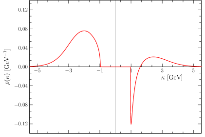
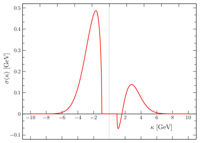
Figure 1: The nonpole part $\overline{\rho}(\kappa)$ of the $\rho(\kappa)$ spectral function, defined in (33), and the $\sigma(\kappa)$ spectral function. The parameters are those in (50).

Figure 2 presents the solutions for the functions $A(p^{2})$, $B(p^{2})$ and $M(p^{2})=B(p^{2})/A(p^{2})$ defined in (4). The insets in the plots of this figure are zooms into the region of the threshold of a branch cut, a cusp at $p^{2}=(M_{p}+\varsigma)^{2}$. This threshold exists because of the pole in (46). The existence of such a cusp, or of more cusps, is a universal feature that will appear with any model in which poles exist in the quark-gluon kernel. For example, with a “Landau-gauge” Ansatz, where the $\gamma^{\mu}$ in (45) is replaced by $(g^{\mu\nu}-q^{\mu}q^{\nu}/q^{2})\gamma_{\nu}$, one more cusp appears at $p^{2}=M^{2}_{p}$, which obviously comes from the $1/q^{2}$ in this expression. Such two-cusp structure is clearly seen in the corresponding plots in Refs. [17,​ 19] in which the Landau gauge is used. Certainly, depending on the complexity of the analytic structure of the quark-gluon kernel, one can expect an even more interesting analytic structure in these functions for $p^{2}>0$.

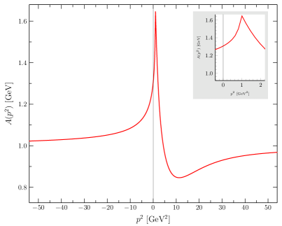
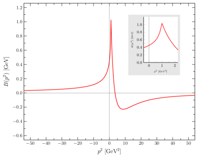
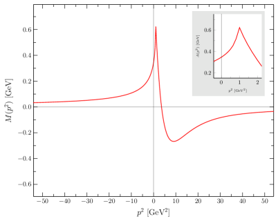
Figure 2: The $A(p^{2})$, $B(p^{2})$ and $M(p^{2})$ functions defined in (4). The insets zoom into the region around the threshold momentum $p^{2}=(M+\varsigma)^{2}$. Parameters are the same as for Fig. (1).

It is important to note that the positivity violation obtained here is not related to the presence of complex-mass poles; for this model-interaction with the parameters in (50), there are no complex-mass poles. A signal for the presence of such complex-mass poles is the violation of the equality in (38), in that the integral over $\rho(\kappa)$ does not vanish [31,​ 32]—in the present calculation, the equality is respected. Complex-mass poles are found in this model, but for parameters very different from those in (50). Moreover, positivity violation is also obtained when using the on-shell renomalization scheme, specified by the equations (41)-(43). In this scheme, the pole mass is set as a renormalization condition. In this scheme, positivity violation also does not depend on the values of the parameters employed. It is also obtained in a one-loop calculation in this scheme. The origin of the positivity violation is again the term $-2\kappa\kappa^{\prime}$, discussed above. Moreover, complex-mass poles are also found in the on-shell scheme for certain values of the parameters. The appearance of such complex-mass poles, in any of the two renormalization schemes, is closely related to the ultraviolet behavior of the quark-gluon kernel: when the interaction is screened in the ultraviolet, the complex-mass poles recede to infinity, in a way very similar to the meson-baryon case investigated in Refs. [32,​ 33,​ 34]. We leave for a future work the investigation of these issues [43].

4 Conclusions and perspectives

We presented a computational method for solving the Dyson-Schwinger equation (DSE) for the quark propagator in Minkowski space. The method uses the spectral representation of the propagator and of its inverse. Instead of solving the DSE for the momentum-dependent mass and renormalization functions, as it is usually solved in its Euclidean formulation, in the spectral method the DSE is solved for the spectral functions. As an application of the formalism, we has used a schematic model for the quark-gluon kernel. Although the model is a very crude representation of the singularity structure of the quark-gluon kernel in Minkowski space, it served the purpose to illustrate important features of the solutions, such as the presence of poles and branch cuts, and positivity violation.

The model calculation served to illustrate in particular the fact that one can obtain positivity violation in the quark propagator in models whose connection to QCD is not a priori clear. We recall that positivity violation in the propagator is conjectured to be relevant for the interpretation of quark confinement, it that it implies that a quark can not be associated with an asymptotic state. We have shown that positive violation is not necessarily related to the presence of complex-mass poles, as they are absent in this model-interaction for the parameters used in the calculation. Moreover, we have pointed out that positivity violation is also obtained in an one-loop perturbative calculation, and is independent of the renormalization conditions. These results have obvious impact for calculations obtaining positivity violation using different models, as it poses the question whether it is a real feature of QCD or of the particular model and of the particular truncation used to solve the DSE.

Future work includes examination of these issues in more realistic models of QCD. One envisages progress with methods based on systematic improvements on a zeroth-order approximation that captures essential features of QCD, examples of which are those of Refs. [43,​ 44,​ 17,​ 45].

- [1] M. Tanabashi, et al., [Particle Data Group], Phys. Rev. D98(3), 030001 (2018). DOI 10.1103/PhysRevD.98.030001
- [2] H. Gies, Lect. Notes Phys. 852, 287 (2012). DOI 10.1007/978-3-642-27320-9˙6
- [3] I.C. Cloet, C.D. Roberts, Prog. Part. Nucl. Phys. 77, 1 (2014). DOI 10.1016/j.ppnp.2014.02.001
- [4] A.C. Aguilar, D. Binosi, J. Papavassiliou, Front. Phys.(Beijing) 11(2), 111203 (2016). DOI 10.1007/s11467-015-0517-6
- [5] G. Eichmann, H. Sanchis-Alepuz, R. Williams, R. Alkofer, C.S. Fischer, Prog. Part. Nucl. Phys. 91, 1 (2016). DOI 10.1016/j.ppnp.2016.07.001
- [6] T. Horn, C.D. Roberts, J. Phys. G43(7), 073001 (2016). DOI 10.1088/0954-3899/43/7/073001
- [7] C.S. Fischer, Prog. Part. Nucl. Phys. 105, 1 (2019). DOI 10.1016/j.ppnp.2019.01.002
- [8] A.G. Williams, G. Krein, C.D. Roberts, Annals Phys. 210, 464 (1991). DOI 10.1016/0003-4916(91)90051-9
- [9] G. Krein, C.D. Roberts, A.G. Williams, Int. J. Mod. Phys. A7, 5607 (1992). DOI 10.1142/S0217751X92002544
- [10] V. Sauli, J. Adam, Jr., Phys. Rev. D67, 085007 (2003). DOI 10.1103/PhysRevD.67.085007
- [11] V. Sauli, JHEP 02, 001 (2003). DOI 10.1088/1126-6708/2003/02/001
- [12] V. Sauli, Few Body Syst. 39, 45 (2006). DOI 10.1007/s00601-006-0156-0
- [13] V. Sauli, J. Adam, Jr., P. Bicudo, Phys. Rev. D75, 087701 (2007). DOI 10.1103/PhysRevD.75.087701
- [14] E.P. Biernat, F. Gross, M.T. Peña, A. Stadler, Few Body Syst. 55, 705 (2014). DOI 10.1007/s00601-014-0863-x
- [15] V. Sauli, J. Phys. G39, 035003 (2012). DOI 10.1088/0954-3899/39/3/035003
- [16] E.P. Biernat, F. Gross, T. Peña, A. Stadler, Phys. Rev. D89(1), 016005 (2014). DOI 10.1103/PhysRevD.89.016005
- [17] F. Siringo, Phys. Rev. D94(11), 114036 (2016). DOI 10.1103/PhysRevD.94.114036
- [18] E.P. Biernat, F. Gross, T. Peña, A. Stadler, S. Leitão, Few Body Syst. 59(5), 80 (2018). DOI 10.1007/s00601-018-1401-z
- [19] F. Siringo, PoS LATTICE2016, 342 (2017). DOI 10.22323/1.256.0342
- [20] G.C. Wick, Phys. Rev. 96, 1124 (1954). DOI 10.1103/PhysRev.96.1124
- [21] C. Itzykson, J.B. Zuber, Quantum Field Theory. International Series In Pure and Applied Physics (McGraw-Hill, New York, 1980). URL http://dx.doi.org/10.1063/1.2916419
- [22] V.A. Karmanov, J. Carbonell, Eur. Phys. J. A27, 1 (2006). DOI 10.1140/epja/i2005-10193-0
- [23] V. Sauli, J. Phys. G35, 035005 (2008). DOI 10.1088/0954-3899/35/3/035005
- [24] J. Carbonell, V.A. Karmanov, Eur. Phys. J. A46, 387 (2010). DOI 10.1140/epja/i2010-11055-4
- [25] V. Sauli, Phys. Rev. D90, 016005 (2014). DOI 10.1103/PhysRevD.90.016005
- [26] J. Carbonell, V.A. Karmanov, Phys. Rev. D90(5), 056002 (2014). DOI 10.1103/PhysRevD.90.056002
- [27] C. Gutierrez, V. Gigante, T. Frederico, G. Salmè, M. Viviani, L. Tomio, Phys. Lett. B759, 131 (2016). DOI 10.1016/j.physletb.2016.05.066
- [28] W. de Paula, T. Frederico, G. Salmè, M. Viviani, Phys. Rev. D94(7), 071901 (2016). DOI 10.1103/PhysRevD.94.071901
- [29] J. Carbonell, T. Frederico, V.A. Karmanov, Eur. Phys. J. C77(1), 58 (2017). DOI 10.1140/epjc/s10052-017-4616-0
- [30] E. Ydrefors, J.H. Alvarenga Nogueira, V.A. Karmanov, T. Frederico, Phys. Lett. B791, 276 (2019). DOI 10.1016/j.physletb.2019.02.046
- [31] W.D. Brown, R.D. Puff, L. Wilets, Phys. Rev. C2, 331 (1970). DOI 10.1103/PhysRevC.2.331
- [32] G. Krein, M. Nielsen, R.D. Puff, L. Wilets, Phys. Rev. C47, 2485 (1993). DOI 10.1103/PhysRevC.47.2485
- [33] M.E. Bracco, A. Eiras, G. Krein, L. Wilets, Phys. Rev. C49, 1299 (1994). DOI 10.1103/PhysRevC.49.1299
- [34] C.A. da Rocha, G. Krein, L. Wilets, Nucl. Phys. A616, 625 (1997). DOI 10.1016/S0375-9474(96)00480-0
- [35] R.A. Tripolt, J. Weyrich, L. von Smekal, J. Wambach, Phys. Rev. D98(9), 094002 (2018). DOI 10.1103/PhysRevD.98.094002
- [36] Z. Wang, L. He, Phys. Rev. D98(9), 094031 (2018). DOI 10.1103/PhysRevD.98.094031
- [37] D.C. Duarte, T. Frederico. Private communication
- [38] S. Jia, M.R. Pennington, Phys. Rev. D96(3), 036021 (2017). DOI 10.1103/PhysRevD.96.036021
- [39] A.S. Kronfeld, Phys. Rev. D58, 051501 (1998). DOI 10.1103/PhysRevD.58.051501
- [40] J.M. Cornwall, Phys. Rev. D26, 1453 (1982). DOI 10.1103/PhysRevD.26.1453
- [41] R. Bermudez, L. Albino, L.X. Gutiérrez-Guerrero, M.E. Tejeda-Yeomans, A. Bashir, Phys. Rev. D95(3), 034041 (2017). DOI 10.1103/PhysRevD.95.034041
- [42] A.C. Aguilar, M.N. Ferreira, C.T. Figueiredo, J. Papavassiliou, Phys. Rev. D99(3), 034026 (2019). DOI 10.1103/PhysRevD.99.034026
- [43] G. Krein, PoS TNT-III, 021 (2013)
- [44] J.L. Kneur, A. Neveu, Phys. Rev. D 92(7), 074027 (2015). DOI 10.1103/PhysRevD.92.074027
- [45] M. Peláez, U. Reinosa, J. Serreau, M. Tissier, N. Wschebor, Phys. Rev. D 96(11), 114011 (2017). DOI 10.1103/PhysRevD.96.114011