AMR Parsing as Sequence-to-Graph Transduction

Abstract

We propose an attention-based model that treats AMR parsing as sequence-to-graph transduction. Unlike most AMR parsers that rely on pre-trained aligners, external semantic resources, or data augmentation, our proposed parser is aligner-free, and it can be effectively trained with limited amounts of labeled AMR data. Our experimental results outperform all previously reported Smatch scores, on both AMR 2.0 (76.3% F1 on LDC2017T10) and AMR 1.0 (70.2% F1 on LDC2014T12).

1 Introduction

Abstract Meaning Representation (AMR, Banarescu et al., 2013) parsing is the task of transducing natural language text into AMR, a graph-based formalism used for capturing sentence-level semantics. Challenges in AMR parsing include: (1) its property of reentrancy – the same concept can participate in multiple relations – which leads to graphs in contrast to trees (Wang et al., 2015); (2) the lack of gold alignments between nodes (concepts) in the graph and words in the text which limits attempts to rely on explicit alignments to generate training data (Flanigan et al., 2014; Wang et al., 2015; Damonte et al., 2017; Foland and Martin, 2017; Peng et al., 2017b; Groschwitz et al., 2018; Guo and Lu, 2018); and (3) relatively limited amounts of labeled data (Konstas et al., 2017).

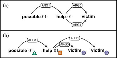
Figure 1: Two views of reentrancy in AMR for an example sentence ``The victim could help himself.'' (a) A standard AMR graph. (b) An AMR tree with node indices as an extra layer of annotation, where the corresponding graph can be recovered by merging nodes of the same index and unioning their incoming edges.

Recent attempts to overcome these challenges include: modeling alignments as latent variables (Lyu and Titov, 2018); leveraging external semantic resources (Artzi et al., 2015; Bjerva et al., 2016); data augmentation (Konstas et al., 2017; van Noord and Bos, 2017b); and employing attention-based sequence-to-sequence models Barzdins and Gosko (2016); Konstas et al. (2017); van Noord and Bos (2017b).

In this paper, we introduce a different way to handle reentrancy, and propose an attention-based model that treats AMR parsing as sequence-to-graph transduction. The proposed model, supported by an extended pointer-generator network, is aligner-free and can be effectively trained with limited amount of labeled AMR data. Experiments on two publicly available AMR benchmarks demonstrate that our parser clearly outperforms the previous best parsers on both benchmarks. It achieves the best reported Smatch scores: 76.3% F1 on LDC2017T10 and 70.2% F1 on LDC2014T12. We also provide extensive ablative and qualitative studies, quantifying the contributions from each component. Our model implementation is available at https://github.com/sheng-z/stog.

2 Another View of Reentrancy

AMR is a rooted, directed, and usually acyclic graph where nodes represent concepts, and labeled directed edges represent the relationships between them (see Figure 1 for an AMR example). The reason for AMR being a graph instead of a tree is that it allows reentrant semantic relations. For instance, in Figure 1(a) ``victim'' is both ARG0 and ARG1 of ``help-01''. While efforts have gone into developing graph-based algorithms for AMR parsing (Chiang et al., 2013; Flanigan et al., 2014), it is more challenging to parse a sentence into an AMR graph rather than a tree as there are efficient off-the-shelf tree-based algorithms, e.g., Chu and Liu (1965); Edmonds (1968). To leverage these tree-based algorithms as well as other structured prediction paradigms McDonald et al. (2005), we introduce another view of reentrancy.

AMR reentrancy is employed when a node participates in multiple semantic relations. We convert an AMR graph into a tree by duplicating nodes that have reentrant relations; that is, whenever a node has a reentrant relation, we make a copy of that node and use the copy to participate in the relation, thereby resulting in a tree. Next, in order to preserve the reentrancy information, we add an extra layer of annotation by assigning an index to each node. Duplicated nodes are assigned the same index as the original node. Figure 1(b) shows a resultant AMR tree: subscripts of nodes are indices; two ``victim'' nodes have the same index as they refer to the same concept. The original AMR graph can be recovered by merging identically indexed nodes and unioning edges from/to these nodes. Similar ideas were used by Artzi et al. (2015) who introduced Skolem IDs to represent anaphoric references in the transformation from CCG to AMR, and van Noord and Bos (2017a) who kept co-indexed AMR variables, and converted them to numbers.

3 Task Formalization

If we consider the AMR tree with indexed nodes as the prediction target, then our approach to parsing is formalized as a two-stage process: node prediction and edge prediction. An example of the parsing process is shown in Figure 2.

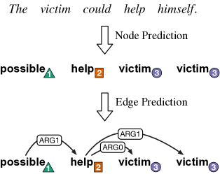
Figure 2: A two-stage process of AMR parsing. We remove senses (i.e., -01, -02, etc.) as they will be assigned in the post-processing step.

Node Prediction Given a input sentence $\bm{w}=\langle w_{1},...,w_{n}\rangle$, each $w_{i}$ a word in the sentence, our approach sequentially decodes a list of nodes $\bm{u}=\langle u_{1},...,u_{m}\rangle$ and deterministically assigns their indices $\bm{d}=\langle d_{1},...,d_{m}\rangle$.

$$P(\bm{u})=\prod_{i=1}^{m}P(u_{i}\mid u_{<i},d_{<i},\bm{w})$$

Note that we allow the same node to occur multiple times in the list; multiple occurrences of a node will be assigned the same index. We choose to predict nodes sequentially rather than simultaneously, because (1) we believe the current node generation is informative to the future node generation; (2) variants of efficient sequence-to-sequence models Bahdanau et al. (2014); Vinyals et al. (2015) can be employed to model this process. At the training time, we obtain the reference list of nodes and their indices using a pre-order traversal over the reference AMR tree. We also evaluate other traversal strategies, and will discuss their difference in Section 7.2.

Figure 3: Extended pointer-generator network for node prediction. For each decoding time step, three probabilities $p_{\textrm{src}}$, $p_{\textrm{tgt}}$ and $p_{\textrm{gen}}$ are calculated. The source and target attention distributions as well as the vocabulary distribution are weighted by these probabilities respectively, and then summed to obtain the final distribution, from which we make our prediction. Best viewed in color.

Edge Prediction Given a input sentence $\bm{w}$, a node list $\bm{u}$, and indices $\bm{d}$, we look for the highest scoring parse tree $y$ in the space $\mathcal{Y}(\bm{u})$ of valid trees over $\bm{u}$ with the constraint of $\bm{d}$. A parse tree $y$ is a set of directed head-modifier edges $y=\{(u_{i},u_{j})\mid 1\leq i,j\leq m\}$. In order to make the search tractable, we follow the arc-factored graph-based approach McDonald et al. (2005); Kiperwasser and Goldberg (2016), decomposing the score of a tree to the sum of the score of its head-modifier edges:

$$\textrm{parse}(\bm{u})=\operatorname*{arg\,max}_{y\in\mathcal{Y}(\bm{u})}\sum_{(u_{i},u_{j})\in y}\textrm{score}(u_{i},u_{j})$$

Based on the scores of the edges, the highest scoring parse tree (i.e., maximum spanning arborescence) can be efficiently found using the Chu-Liu-Edmonnds algorithm. We further incorporate indices as constraints in the algorithm, which is described in Section 4.4. After obtaining the parse tree, we merge identically indexed nodes to recover the standard AMR graph.

4 Model

Our model has two main modules: (1) an extended pointer-generator network for node prediction; and (2) a deep biaffine classifier for edge prediction. The two modules correspond to the two-stage process for AMR parsing, and they are jointly learned during training.

4.1 Extended Pointer-Generator Network

Inspired by the self-copy mechanism in Zhang et al. (2018), we extend the pointer-generator network See et al. (2017) for node prediction. The pointer-generator network was proposed for text summarization, which can copy words from the source text via pointing, while retaining the ability to produce novel words through the generator. The major difference of our extension is that it can copy nodes, not only from the source text, but also from the previously generated nodes on the target side. This target-side pointing is well-suited to our task as nodes we will predict can be copies of other nodes. While there are other pointer/copy networks Gulcehre et al. (2016); Merity et al. (2016); Gu et al. (2016); Miao and Blunsom (2016); Nallapati et al. (2016), we found the pointer-generator network very effective at reducing data sparsity in AMR parsing, which will be shown in Section 7.2.

As depicted in Figure 3, the extended pointer-generator network consists of four major components: an encoder embedding layer, an encoder, a decoder embedding layer, and a decoder.

Encoder Embedding Layer This layer converts words in input sentences into vector representations. Each vector is the concatenation of embeddings of GloVe Pennington et al. (2014), BERT Devlin et al. (2018), POS (part-of-speech) tags and anonymization indicators, and features learned by a character-level convolutional neural network (CharCNN, Kim et al., 2016).

Anonymization indicators are binary indicators that tell the encoder whether the word is an anonymized word. In preprocessing, text spans of named entities in input sentences will be replaced by anonymized tokens (e.g. person, country) to reduce sparsity (see the Appendix for details).

Except BERT, all other embeddings are fetched from their corresponding learned embedding look-up tables. BERT takes subword units as input, which means that one word may correspond to multiple hidden states of BERT. In order to accurately use these hidden states to represent each word, we apply an average pooling function to the outputs of BERT. Figure 4 illustrates the process of generating word-level embeddings from BERT.

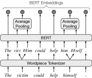
Figure 4: Word-level embeddings from BERT.

Encoder The encoder is a multi-layer bidirectional RNN Schuster and Paliwal (1997):

$$\bm{h}^{l}_{i}=[\overrightarrow{f}^{l}(\bm{h}^{l-1}_{i},\bm{h}^{l}_{i-1});\overleftarrow{f}^{l}(\bm{h}^{l-1}_{i},\bm{h}^{l}_{i+1})],$$

where $\overrightarrow{f}^{l}$ and $\overleftarrow{f}^{l}$ are two LSTM cells Hochreiter and Schmidhuber (1997); $\bm{h}^{l}_{i}$ is the $l$-th layer encoder hidden state at the time step $i$; $\bm{h}^{0}_{i}$ is the encoder embedding layer output for word $w_{i}$.

Decoder Embedding Layer Similar to the encoder embedding layer, this layer outputs vector representations for AMR nodes. The difference is that each vector is the concatenation of embeddings of GloVe, POS tags and indices, and feature vectors from CharCNN.

POS tags of nodes are inferred at runtime: if a node is a copy from the input sentence, the POS tag of the corresponding word is used; if a node is a copy from the preceding nodes, the POS tag of its antecedent is used; if a node is a new node emitted from the vocabulary, an UNK tag is used.

We do not include BERT embeddings in this layer because AMR nodes, especially their order, are significantly different from natural language text (on which BERT was pre-trained). We tried to use ``fixed'' BERT in this layer, which did not lead to improvement.

Decoder At each step $t$, the decoder (an $l$-layer unidirectional LSTM) receives hidden state $\bm{s}^{l-1}_{t}$ from the last layer and hidden state $\bm{s}^{l}_{t-1}$ from the previous time step, and generates hidden state $\bm{s}^{l}_{t}$:

$$\bm{s}^{l}_{t}=f^{l}(\bm{s}^{l-1}_{t},\bm{s}^{l}_{t-1}),$$

where $\bm{s}^{0}_{t}$ is the concatenation (i.e., the input-feeding approach, Luong et al., 2015) of two vectors: the decoder embedding layer output for the previous node $u_{t-1}$ (while training, $u_{t-1}$ is the previous node of the reference node list; at test time it is the previous node emitted by the decoder), and the attentional vector $\widetilde{\bm{s}}_{t-1}$ from the previous step (explained later in this section). $\bm{s}^{l}_{0}$ is the concatenation of last encoder hidden states from $\overrightarrow{f}^{l}$ and $\overleftarrow{f}^{l}$ respectively.

Source attention distribution $\bm{a}^{t}_{\textrm{src}}$ is calculated by additive attention Bahdanau et al. (2014):

$$\bm{e}^{t}_{\textrm{src}}= ~{}\bm{v}^{\top}_{\textrm{src}}\textrm{tanh}(\bm{W}_{\textrm{src}}\bm{h}^{l}_{1:n}+\bm{U}_{\textrm{src}}\bm{s}^{l}_{t}+\bm{b}_{\textrm{src}}),$$

$$\bm{a}^{t}_{\textrm{src}}= ~{}\textrm{softmax}(\bm{e}^{t}_{\textrm{src}}),$$

and it is then used to produce a weighted sum of encoder hidden states, i.e., the context vector $\bm{c}_{t}$.

Attentional vector $\widetilde{\bm{s}}_{t}$ combines both source and target side information, and it is calculated by an MLP (shown in Figure 3):

$$\widetilde{\bm{s}}_{t}=\textrm{tanh}(\bm{W}_{c}[\bm{c}_{t};\bm{s}^{l}_{t}]+\bm{b}_{c})$$

The attentional vector $\widetilde{\bm{s}}_{t}$ has 3 usages:

(1) it is fed through a linear layer and softmax to produce the vocabulary distribution:

$$P_{\textrm{vocab}}=\textrm{softmax}(\bm{W}_{\textrm{vocab}}\widetilde{\bm{s}}_{t}+\bm{b}_{\textrm{vocab}})$$

(2) it is used to calculate the target attention distribution $\bm{a}^{t}_{\textrm{tgt}}$:

$$\bm{e}^{t}_{\textrm{tgt}}= ~{}\bm{v}^{\top}_{\textrm{tgt}}\textrm{tanh}(\bm{W}_{\textrm{tgt}}\widetilde{\bm{s}}_{1:t-1}+\bm{U}_{\textrm{tgt}}\widetilde{\bm{s}}_{t}+\bm{b}_{\textrm{tgt}}),$$

$$\bm{a}^{t}_{\textrm{tgt}}= ~{}\textrm{softmax}(\bm{e}^{t}_{\textrm{tgt}}),$$

(3) it is used to calculate source-side copy probability $p_{\textrm{src}}$, target-side copy probability $p_{\textrm{tgt}}$, and generation probability $p_{\textrm{gen}}$ via a switch layer:

$$[p_{\textrm{src}},p_{\textrm{tgt}},p_{\textrm{gen}}]=\textrm{softmax}(\bm{W}_{\textrm{switch}}\widetilde{\bm{s}}_{t}+\bm{b}_{\textrm{switch}})$$

Note that $p_{\textrm{src}}+p_{\textrm{tgt}}+p_{\textrm{gen}}=1$. They act as a soft switch to choose between copying an existing node from the preceding nodes by sampling from the target attention distribution $\bm{a}^{t}_{\textrm{tgt}}$, or emitting a new node in two ways: (1) generating a new node from the fixed vocabulary by sampling from $P_{\textrm{vocab}}$, or (2) copying a word (as a new node) from the input sentence by sampling from the source attention distribution $\bm{a}^{t}_{\textrm{src}}$.

The final probability distribution $P^{\textrm{(node)}}(u_{t})$ for node $u_{t}$ is defined as follows. If $u_{t}$ is a copy of existing nodes, then:

$$P^{\textrm{(node)}}(u_{t})=p_{\textrm{tgt}}\sum_{i:u_{i}=u_{t}}^{t-1}\bm{a}^{t}_{\textrm{tgt}}[i],$$

otherwise:

$$P^{\textrm{(node)}}(u_{t})=p_{\textrm{gen}}P_{\textrm{vocab}}(u_{t})+p_{\textrm{src}}\sum_{i:w_{i}=u_{t}}^{n}\bm{a}^{t}_{\textrm{src}}[i],$$

where $\bm{a}^{t}[i]$ indexes the $i$-th element of $\bm{a}^{t}$. Note that a new node may have the same surface form as the existing node. We track their difference using indices. The index $d_{t}$ for node $u_{t}$ is assigned deterministically as below:

$$d_{t}=\left\{\begin{aligned} t,&\ \textrm{if}\ u_{t}\textrm{ is a new node;}\\ d_{j},&\ \textrm{if}\ u_{t}\textrm{ is a copy of its antecedent }u_{j}\textrm{.}\end{aligned}\right.$$

4.2 Deep Biaffine Classifier

For the second stage (i.e., edge prediction), we employ a deep biaffine classifier, which was originally proposed for graph-based dependency parsing Dozat and Manning (2016), and recently has been applied to semantic parsing Peng et al. (2017a); Dozat and Manning (2018).

As depicted in Figure 5, the major difference of our usage is that instead of re-encoding AMR nodes, we directly use decoder hidden states from the extended pointer-generator network as the input to deep biaffine classifier. We find two advantages of using decoder hidden states as input: (1) through the input-feeding approach, decoder hidden states contain contextualized information from both the input sentence and the predicted nodes; (2) because decoder hidden states are used for both node prediction and edge prediction, we can jointly train the two modules in our model.

Given decoder hidden states $\langle\bm{s}_{1},...,\bm{s}_{m}\rangle$ and a learnt vector representation $\bm{s}^{\prime}_{0}$ of a dummy root, we follow Dozat and Manning (2016), factorizing edge prediction into two components: one that predicts whether or not a directed edge $(u_{k},u_{t})$ exists between two nodes $u_{k}$ and $u_{t}$, and another that predicts the best label for each potential edge.

Edge and label scores are calculated as below:

$$\bm{s}^{\textrm{(edge-head)}}_{t}=\textrm{MLP}^{\textrm{(edge-head)}}(\bm{s}_{t})$$

$$\bm{s}^{\textrm{(edge-dep)}}_{t}=\textrm{MLP}^{\textrm{(edge-dep)}}(\bm{s}_{t})$$

$$\bm{s}^{\textrm{(label-head)}}_{t}=\textrm{MLP}^{\textrm{(label-head)}}(\bm{s}_{t})$$

$$\bm{s}^{\textrm{(label-dep)}}_{t}=\textrm{MLP}^{\textrm{(label-dep)}}(\bm{s}_{t})$$

$$\textrm{score}^{\textrm{(edge)}}_{k,t}=\textrm{Biaffine}(\bm{s}^{\textrm{(edge-head)}}_{k},\bm{s}^{\textrm{(edge-dep)}}_{t})$$

$$\textrm{score}^{\textrm{(label)}}_{k,t}=\textrm{Bilinear}(\bm{s}^{\textrm{(label-head)}}_{k},\bm{s}^{\textrm{(label-dep)}}_{t})$$

where MLP, Biaffine and Bilinear are defined as below:

$$\textrm{MLP}(\bm{x})=\textrm{ELU}(\bm{W}\bm{x}+\bm{b})$$

$$\textrm{Biaffine}(\bm{x}_{1},\bm{x}_{2})=\bm{x}^{\top}_{1}\bm{U}\bm{x}_{2}+\bm{W}[\bm{x}_{1};\bm{x}_{2}]+\bm{b}$$

$$\textrm{Bilinear}(\bm{x}_{1},\bm{x}_{2})=\bm{x}^{\top}_{1}\bm{U}\bm{x}_{2}+\bm{b}$$

Given a node $u_{t}$, the probability of $u_{k}$ being the edge head of $u_{t}$ is defined as:

$$P^{\textrm{(head)}}_{t}(u_{k})=\frac{\exp(\textrm{score}^{\textrm{(edge)}}_{k,t})}{\sum_{j=1}^{m}\exp(\textrm{score}^{\textrm{(edge)}}_{j,t})}$$

The edge label probability for edge $(u_{k},u_{t})$ is defined as:

$$P^{\textrm{(label)}}_{k,t}(l)=\frac{\exp(\textrm{score}^{\textrm{(label)}}_{k,t}[l])}{\sum_{l^{\prime}}\exp(\textrm{score}^{\textrm{(label)}}_{k,t}[l^{\prime}])}$$

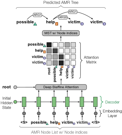
Figure 5: Deep biaffine classifier for edge prediction. Edge label prediction is not depicted in the figure.

4.3 Training

The training objective is to jointly minimize the loss of reference nodes and edges, which can be decomposed to the sum of the negative log likelihood at each time step $t$ for (1) the reference node $u_{t}$, (2) the reference edge head $u_{k}$ of node $u_{t}$, and (3) the reference edge label $l$ between $u_{k}$ and $u_{t}$:

$$\textrm{minimize}-\sum_{t=1}^{m} [\log{P^{\textrm{(node)}}(u_{t})}+\log{P^{\textrm{(head)}}_{t}(u_{k})}$$

$$+\log{P^{\textrm{(label)}}_{k,t}(l)}+\lambda\textrm{covloss}_{t}]$$

$\textrm{covloss}_{t}$ is a coverage loss to penalize repetitive nodes: $\textrm{covloss}_{t}=\sum_{i}\textrm{min}(\bm{a}^{t}_{\textrm{src}}[i],\textbf{cov}^{t}[i])$, where $\textbf{cov}^{t}$ is the sum of source attention distributions over all previous decoding time steps: $\textbf{cov}^{t}=\sum_{t^{\prime}=0}^{t-1}\bm{a}^{t^{\prime}}_{\textrm{src}}$. See See et al. (2017) for full details.

4.4 Prediction

For node prediction, based on the final probability distribution $P^{\textrm{(node)}}(u_{t})$ at each decoding time step, we implement both greedy search and beam search to sequentially decode a node list $\bm{u}$ and indices $\bm{d}$.

For edge prediction, given the predicted node list $\bm{u}$, their indices $\bm{d}$, and the edge scores $S=\{\textrm{score}^{\textrm{(edge)}}_{i,j}\mid 0\leq i,j\leq m\}$, we apply the Chu-Liu-Edmonds algorithm with a simple adaption to find the maximum spanning tree (MST). As described in Algorithm 1, before calling the Chu-Liu-Edmonds algorithm, we first include a dummy root $u_{0}$ to ensure every node have a head, and then exclude edges whose source and destination nodes have the same indices, because these nodes will be merged into a single node to recover the standard AMR graph where self-loops are invalid.

Input : Nodes $\bm{u}=\langle u_{1},...,u_{m}\rangle$,

Indices $\bm{d}=\langle d_{1},...d_{m}\rangle$,

Edge scores $S=\{\textrm{score}^{\textrm{(edge)}}_{i,j}\mid 0\leq i,j\leq m\}$

Output : A maximum spanning tree.

// Include the dummy root $u_{0}$.

$V\leftarrow\{u_{0}\}\cup\bm{u}$;

$d_{0}\leftarrow 0$;

// Exclude invalid edges.

// $d_{i}$ is the node index for node $u_{i}$.

$E\leftarrow\{(u_{i},u_{j})\mid 0\leq i,j\leq m;d_{i}\neq d_{j}\}$;

// Chu-Liu-Edmonds algorithm

return MST($V,E,S,u_{0}$);

Algorithm 1 Chu-Liu-Edmonds algo. w/ Adaption

5 Related Work

AMR parsing approaches can be categorized into alignment-based, transition-based, grammar-based, and attention-based approaches.

Alignment-based approaches were first explored by JAMR Flanigan et al. (2014), a pipeline of concept and relation identification with a graph-based algorithm. Zhou et al. (2016) improved this by jointly learning concept and relation identification with an incremental model. Both approaches rely on features based on alignments. Lyu and Titov (2018) treated alignments as latent variables in a joint probabilistic model, leading to a substantial reported improvement. Our approach requires no explicit alignments, but implicitly learns a source-side copy mechanism using attention.

Transition-based approaches began with Wang et al. (2015, 2016), who incrementally transform dependency parses into AMRs using transiton-based models, which was followed by a line of research, such as Puzikov et al. (2016); Brandt et al. (2016); Goodman et al. (2016); Damonte et al. (2017); Ballesteros and Al-Onaizan (2017); Groschwitz et al. (2018). A pre-trained aligner, e.g. Pourdamghani et al. (2014); Liu et al. (2018), is needed for most parsers to generate training data (e.g., oracles for a transition-based parser). Our approach makes no significant use of external semantic resources, and is aligner-free.

Grammar-based approaches are represented by Artzi et al. (2015); Peng et al. (2015) who leveraged external semantic resources, and employed CCG-based or SHRG-based grammar induction approaches converting logical forms into AMRs. Pust et al. (2015) recast AMR parsing as a machine translation problem, while also drawing features from external semantic resources.

Attention-based parsing with Seq2Seq-style models have been considered Barzdins and Gosko (2016); Peng et al. (2017b), but are limited by the relatively small amount of labeled AMR data. Konstas et al. (2017) overcame this by making use of millions of unlabeled data through self-training, while van Noord and Bos (2017b) showed significant gains via a character-level Seq2Seq model and a large amount of silver-standard AMR training data. In contrast, our approach supported by extended pointer generator can be effectively trained on the limited amount of labeled AMR data, with no data augmentation.

6 AMR Pre- and Post-processing

Anonymization is often used in AMR preprocessing to reduce sparsity (Werling et al., 2015; Peng et al., 2017b; Guo and Lu, 2018, inter alia). Similar to Konstas et al. (2017), we anonymize sub-graphs of named entities and other entities. Like Lyu and Titov (2018), we remove senses, and use Stanford CoreNLP Manning et al. (2014) to lemmatize input sentences and add POS tags.

In post-processing, we assign the most frequent sense for nodes (-01, if unseen) like Lyu and Titov (2018), and restore wiki links using the DBpedia Spotlight API Daiber et al. (2013) following Bjerva et al. (2016); van Noord and Bos (2017b). We add polarity attributes based on the rules observed from the training data. More details of pre- and post-processing are provided in the Appendix.

7 Experiments

7.1 Setup

GloVe.840B.300d embeddings
dim	300
BERT embeddings
source	BERT-Large-cased
dim	1024
POS tag embeddings
dim	100
Anonymization indicator embeddings
dim	50
Index embeddings
dim	50
CharCNN
num_filters	100
ngram_filter_sizes	[3]
Encoder
hidden_size	512
num_layers	2
Decoder
hidden_size	1024
num_layers	2
Deep biaffine classifier
edge_hidden_size	256
label_hidden_size	128
Optimizer
type	ADAM
learning_rate	0.001
max_grad_norm	5.0
Coverage loss weight $\lambda$	1.0
Beam size	5
Vocabulary
encoder_vocab_size (AMR 2.0)	18000
decoder_vocab_size (AMR 2.0)	12200
encoder_vocab_size (AMR 1.0)	9200
decoder_vocab_size (AMR 1.0)	7300
Batch size	64

Table 1: Hyper-parameter settings

We conduct experiments on two AMR general releases (available to all LDC subscribers): AMR 2.0 (LDC2017T10) and AMR 1.0 (LDC2014T12). Our model is trained using ADAM Kingma and Ba (2014) for up to 120 epochs, with early stopping based on the development set. Full model training takes about 19 hours on AMR 2.0 and 7 hours on AMR 1.0, using two GeForce GTX TITAN X GPUs. At training, we have to fix BERT parameters due to the limited GPU memory. We leave fine-tuning BERT for future work.

Table 1 lists the hyper-parameters used in our full model. Both encoder and decoder embedding layers have GloVe and POS tag embeddings as well as CharCNN, but their parameters are not tied. We apply dropout (dropout_rate = 0.33) to the outputs of each module.

7.2 Results

Corpus	Parser	F1(%)
AMR 2.0	Buys and Blunsom (2017)	61.9
	van Noord and Bos (2017b)	71.0∗
	Groschwitz et al. (2018)	71.0$\pm$0.5
	Lyu and Titov (2018)	74.4$\pm$0.2
	Naseem et al. (2019)	75.5
	Ours	76.3$\pm$0.1
AMR 1.0	Flanigan et al. (2016)	66.0
	Pust et al. (2015)	67.1
	Wang and Xue (2017)	68.1
	Guo and Lu (2018)	68.3$\pm$0.4
	Ours	70.2$\pm$0.1

Table 2: Smatch scores on the test sets of AMR 2.0 and 1.0. Standard deviation is computed over 3 runs with different random seeds. ^∗ indicates the previous best score from attention-based models.

Main Results We compare our approach against the previous best approaches and several recent competitors. Table 2 summarizes their Smatch scores Cai and Knight (2013) on the test sets of two AMR general releases. On AMR 2.0, we outperform the latest push from Naseem et al. (2019) by 0.8% F1, and significantly improves Lyu and Titov (2018)'s results by 1.9% F1. Compared to the previous best attention-based approach van Noord and Bos (2017b), our approach shows a substantial gain of 5.3% F1, with no usage of any silver-standard training data. On AMR 1.0 where the traininng instances are only around 10k, we improve the best reported results by 1.9% F1.

Fine-grained Results In Table 3, we assess the quality of each subtask using the AMR-evaluation tools Damonte et al. (2017). We see a notable increase on reentrancies, which we attribute to target-side copy (based on our ablation studies in the next section). Significant increases are also shown on wikification and negation, indicating the benefits of using DBpedia Spotlight API and negation detection rules in post-processing. On all other subtasks except named entities, our approach achieves competitive results to the previous best approaches Lyu and Titov (2018); Naseem et al. (2019), and outperforms the previous best attention-based approach van Noord and Bos (2017b). The difference of scores on named entities is mainly caused by anonymization methods used in preprocessing, which suggests a potential improvement by adapting the anonymization method presented in Lyu and Titov (2018) to our approach.

Metric	vN'18	L'18	N'19	Ours
Smatch	71.0	74.4	75.5	76.3$\pm$0.1
Unlabeled	74	77	80	79.0$\pm$0.1
No WSD	72	76	76	76.8$\pm$0.1
Reentrancies	52	52	56	60.0$\pm$0.1
Concepts	82	86	86	84.8$\pm$0.1
Named Ent.	79	86	83	77.9$\pm$0.2
Wikification	65	76	80	85.8$\pm$0.3
Negation	62	58	67	75.2$\pm$0.2
SRL	66	70	72	69.7$\pm$0.2

Table 3: Fine-grained F1 scores on the AMR 2.0 test set. vN'17 is van Noord and Bos (2017b); L'18 is Lyu and Titov (2018); N'19 is Naseem et al. (2019).

Ablation	AMR 1.0	AMR 2.0
Full model	70.2	76.3
no source-side copy	62.7	70.9
no target-side copy	66.2	71.6
no coverage loss	68.5	74.5
no BERT embeddings	68.8	74.6
no index embeddings	68.5	75.5
no anonym. indicator embed.	68.9	75.6
no beam search	69.2	75.3
no POS tag embeddings	69.2	75.7
no CharCNN features	70.0	75.8
only edge prediction	88.4	90.9

Table 4: Ablation studies on components of our model. (Scores are sorted by the delta from the full model.)

Ablation Study We consider the contributions of several model components in Table 4. The largest performance drop is from removing source-side copy, showing its efficiency at reducing sparsity from open-class vocabulary entries. Removing target-side copy also leads to a large drop. Specifically, the subtask score of reentrancies drops down to 38.4% when target-side copy is disabled. Coverage loss is useful with regard to discouraging unnecessary repetitive nodes. In addition, our model benefits from input features such as language representations from BERT, index embeddings, POS tags, anonymization indicators, and character-level features from CharCNN. Note that without BERT embeddings, our model still outperforms the previous best approaches (Lyu and Titov, 2018; Guo and Lu, 2018) that are not using BERT. Beam search, commonly used in machine translation, is also helpful in our model. We provide side-by-side examples in the Appendix to further illustrate the contribution from each component, which are largely intuitive, with the exception of BERT embeddings. There the exact contribution of the component (qualitative, before/after ablation) stands out less: future work might consider a probing analysis with manually constructed examples, in the spirit of Linzen et al. (2016); Conneau et al. (2018); Tenney et al. (2019).

In the last row, we only evaluate model performance at the edge prediction stage by forcing our model to decode the reference nodes at the node prediction stage. The results mean if our model could make perfect prediction at the node prediction stage, the final Smatch score will be substantially high, which identifies node prediction as the key to future improvement of our model.

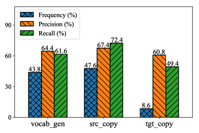
Figure 6: Frequency, precision and recall of nodes from different sources, based on the AMR 2.0 test set.

There are three sources for node prediction: vocabulary generation, source-side copy, or target-side copy. Let all reference nodes from source $z$ be $N^{(z)}_{\text{ref}}$, and all system predicted nodes from $z$ be $N^{(z)}_{\text{sys}}$. we compute frequency, precision and recall of nodes from source $z$ as below:

$$\left.\textrm{frequency}^{(z)}={|N^{(z)}_{\text{ref}}|}\middle/{\sum\nolimits_{z}|N^{(z)}_{\text{ref}}|}\right.$$

$$\left.\textrm{precision}^{(z)}={|N^{(z)}_{\text{ref}}\cap N^{(z)}_{\text{sys}}|}\middle/{|N^{(z)}_{\text{sys}}|}\right.$$

$$\left.\textrm{recall}^{(z)}={|N^{(z)}_{\text{ref}}\cap N^{(z)}_{\text{sys}}|}\middle/{|N^{(z)}_{\text{ref}}|}\right.$$

Figure 6 shows the frequency of nodes from difference sources, and their corresponding precision and recall based on our model prediction. Among all reference nodes, 43.8% are from vocabulary generation, 47.6% from source-side copy, and only 8.6% from target-side copy. On one hand, the highest frequency of source-side copy helps address sparsity and results in the highest precision and recall. On the other hand, we see space for improvement, especially on the relatively low recall of target-side copy, which is probably due to its low frequency.

Node Linearization As decribed in Section 3, we create the reference node list by a pre-order traversal over the gold AMR tree. As for the children of each node, we sort them in alphanumerical order. This linearization strategy has two advantages: (1) pre-order traversal guarantees that a head node (predicate) always comes in front of its children (arguments); (2) alphanumerical sort orders according to role ID (i.e., ARG0>ARG1>…>ARGn), following intuition from research in Thematic Hierarchies Fillmore (1968); Levin and Hovav (2005).

Node Linearization	AMR 1.0	AMR 2.0
Pre-order + Alphanum	70.2	76.3
Pre-order + Alignment	61.9	68.3
Pure Alignment	64.3	71.3

Table 5: Smatch scores of full models trained and tested based on different node linearization strategies.

In Table 5, we report Smatch scores of full models trained and tested on data generated via our linearization strategy (Pre-order + Alphanum), as compared to two obvious alternates: the first alternate still runs a pre-order traversal, but it sorts the children of each node based on the their alignments to input words; the second one linearizes nodes purely based alignments. Alignments are created using the tool by Pourdamghani et al. (2014). Clearly, our linearization strategy leads to much better results than the two alternates. We also tried other traversal strategies such as combining in-order traversal with alphanumerical sorting or alignment-based sorting, but did not get scores even comparable to the two alternates.

Average Pooling vs. Max Pooling In Figure 4, we apply average pooling to the outputs (last-layer hidden states) of BERT in order to generate word-level embeddings for the input sentence. Table 6 shows scores of models using different pooling functions. Average pooling performs slightly better than max pooling.

	AMR 1.0	AMR 2.0
Average Pooling	70.2$\pm$0.1	76.3$\pm$0.1
Max Pooling	70.0$\pm$0.1	76.2$\pm$0.1

Table 6: Smatch scores based different pooling functions. Standard deviation is over 3 runs on the test data.

8 Conclusion

We proposed an attention-based model for AMR parsing where we introduced a series of novel components into a transductive setting that extend beyond what a typical NMT system would do on this task. Our model achieves the best performance on two AMR corpora. For future work, we would like to extend our model to other semantic parsing tasks Oepen et al. (2014); Abend and Rappoport (2013). We are also interested in semantic parsing in cross-lingual settings Zhang et al. (2018); Damonte and Cohen (2018).

Appendix A Appendices

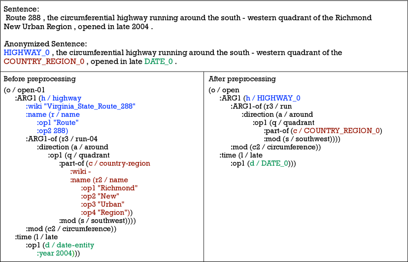
Figure 7: An example AMR and the corresponding sentence before and after preprocessing. Senses are removed. The first named entity is replaced by ``HIGHWAY_0''; the second named entity is replaced by ``COUNTRY_REGION_0''; the first date entity replaced by ``DATE_0''.

A.1 AMR Pre- and Post-processing

Firstly, we to run Standford CoreNLP like Lyu and Titov (2018), lemmatizing input sentences and adding POS tags to each token. Secondly, we remove senses, wiki links and polarity attributes in AMR. Thirdly, we anonymize sub-graphs of named entities and *-entity in a way similar to Konstas et al. (2017). Figure 7 shows an example before and after preprocessing. Sub-graphs of named entities are headed by one of AMR's fine-grained entity types (e.g., highway, country_region in Figure 7) that contain a :name role. Sub-graphs of other entities are headed by their corresponding entity type name (e.g., date-entity in Figure 7). We replace these sub-graphs with a token of a special pattern ``TYPE_i'' (e.g. HIGHWAY_0, DATE_0 in Figure 7), where ``TYPE" indicates the AMR entity type of the corresponding sub-graph, and ``i'' indicates that it is the $i$-th occurrence of that type. On the training set, we use simple rules to find mappings between anonymized sub-graphs and spans of text, and then replace mapped text with the anonymized token we inserted into the AMR graph. Additionally, we build a mapping of Standford CoreNLP NER tags to AMR's fine-grained types based on the training set, which will be used in prediction. At test time, we normalize sentences to match our anonymized training data. For any entity span identified by Stanford CoreNLP, we replace it with a AMR entity type based on the mapping built during training. If no entry is found in the mapping, we replace entity spans with the coarse-grained NER tags from Stanford CoreNLP, which are also entity types in AMR.

In post-processing, we deterministically generate AMR sub-graphs for anonymizations using the corresponding text span. We assign the most frequent sense for nodes (-01, if unseen) like Lyu and Titov (2018). We add wiki links to named entities using the DBpedia Spotlight API Daiber et al. (2013) following Bjerva et al. (2016); van Noord and Bos (2017b) with the confidence threshod at 0.5. We add polarity attributes based on Algorithm 2 where the four functions isNegation, modifiedWord, mappedNode, and addPolarity consists of simple rules observed from the training set. We use the PENMANCodec to encode and decode both intermediate and final AMRs.

Input : Sent. $\bm{w}=\langle w_{1},...,w_{n}\rangle$, Predicted AMR $A$

Output : AMR with polarity attributes.

for $w_{i}\in\bm{w}$ do

       if isNegation($w_{i}$) then

             $w_{j}\leftarrow$ modifiedWord($w_{i}$, $\bm{w}$);

             $u_{k}\leftarrow$ mappedNode($w_{j}$, $A$);

             $A\leftarrow$ addPolarity($u_{k}$, $A$);

            

       end if

      

end for

return $A$;

Algorithm 2 Adding polarity attributes to AMR.

A.2 Side-by-Side Examples

In the next page, we provide examples from the test set, with side-by-side comparisons between the full model prediction and the model prediction after ablation.

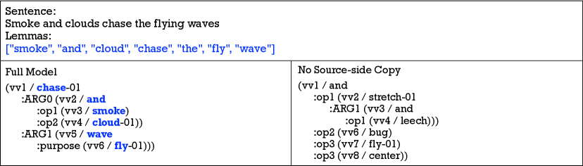
Figure 8: Full model prediction vs. no source-side copy prediction. Tokens in blue are copied from the source side. Without source-side copy, the prediction becomes totally different and inaccurate in this example.

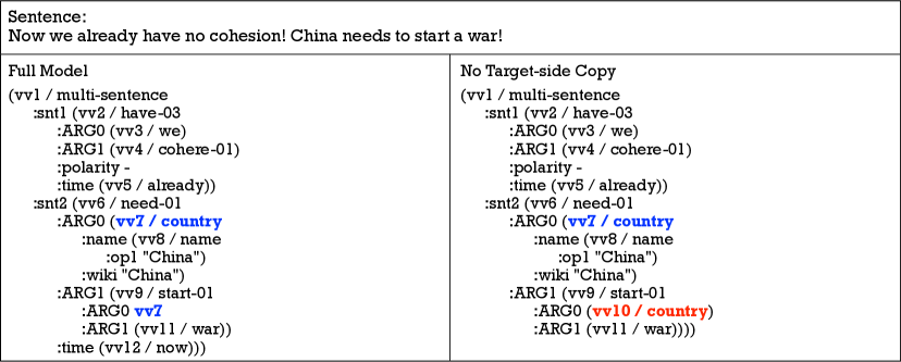
Figure 9: Full model prediction vs. no target-side copy prediction. Nodes in blue denote the same concept (i.e., the country ``China''). The full model correctly copies the first node (``vv7 / country'') as ARG0 of ``start-01''. Without target-side copy, the model has to generate a new node with a different index, i.e., ``vv10 / country''.

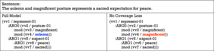
Figure 10: Full model prediction vs. no coverage loss prediction. The full model correctly predicts the second modifier ``solemn''. Without coverage loss, the model generates a repetitive modifier ``magnificent''.

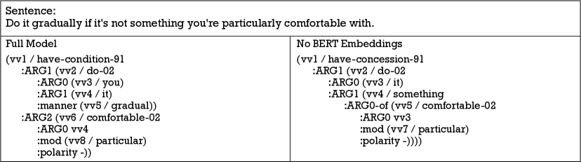
Figure 11: Full model prediction vs. no BERT embeddings prediction.

References

- Abend and Rappoport (2013) Omri Abend and Ari Rappoport. 2013. Universal conceptual cognitive annotation (ucca). In Proceedings of the 51st Annual Meeting of the Association for Computational Linguistics (Volume 1: Long Papers), pages 228–238. Association for Computational Linguistics.
- Artzi et al. (2015) Yoav Artzi, Kenton Lee, and Luke Zettlemoyer. 2015. Broad-coverage ccg semantic parsing with amr. In Proceedings of the 2015 Conference on Empirical Methods in Natural Language Processing, pages 1699–1710. Association for Computational Linguistics.
- Bahdanau et al. (2014) Dzmitry Bahdanau, Kyunghyun Cho, and Yoshua Bengio. 2014. Neural machine translation by jointly learning to align and translate. arXiv preprint arXiv:1409.0473.
- Ballesteros and Al-Onaizan (2017) Miguel Ballesteros and Yaser Al-Onaizan. 2017. AMR parsing using stack-LSTMs. In Proceedings of the 2017 Conference on Empirical Methods in Natural Language Processing, pages 1269–1275, Copenhagen, Denmark. Association for Computational Linguistics.
- Banarescu et al. (2013) Laura Banarescu, Claire Bonial, Shu Cai, Madalina Georgescu, Kira Griffitt, Ulf Hermjakob, Kevin Knight, Philipp Koehn, Martha Palmer, and Nathan Schneider. 2013. Abstract meaning representation for sembanking. In Proceedings of the 7th Linguistic Annotation Workshop and Interoperability with Discourse, pages 178–186. Association for Computational Linguistics.
- Barzdins and Gosko (2016) Guntis Barzdins and Didzis Gosko. 2016. Riga at semeval-2016 task 8: Impact of smatch extensions and character-level neural translation on amr parsing accuracy. In Proceedings of the 10th International Workshop on Semantic Evaluation (SemEval-2016), pages 1143–1147. Association for Computational Linguistics.
- Bjerva et al. (2016) Johannes Bjerva, Johan Bos, and Hessel Haagsma. 2016. The meaning factory at semeval-2016 task 8: Producing amrs with boxer. In Proceedings of the 10th International Workshop on Semantic Evaluation (SemEval-2016), pages 1179–1184. Association for Computational Linguistics.
- Brandt et al. (2016) Lauritz Brandt, David Grimm, Mengfei Zhou, and Yannick Versley. 2016. Icl-hd at semeval-2016 task 8: Meaning representation parsing - augmenting amr parsing with a preposition semantic role labeling neural network. In Proceedings of the 10th International Workshop on Semantic Evaluation (SemEval-2016), pages 1160–1166. Association for Computational Linguistics.
- Buys and Blunsom (2017) Jan Buys and Phil Blunsom. 2017. Oxford at semeval-2017 task 9: Neural amr parsing with pointer-augmented attention. In Proceedings of the 11th International Workshop on Semantic Evaluation (SemEval-2017), pages 914–919. Association for Computational Linguistics.
- Cai and Knight (2013) Shu Cai and Kevin Knight. 2013. Smatch: an evaluation metric for semantic feature structures. In Proceedings of the 51st Annual Meeting of the Association for Computational Linguistics (Volume 2: Short Papers), pages 748–752. Association for Computational Linguistics.
- Chiang et al. (2013) David Chiang, Jacob Andreas, Daniel Bauer, Karl Moritz Hermann, Bevan Jones, and Kevin Knight. 2013. Parsing graphs with hyperedge replacement grammars. In Proceedings of the 51st Annual Meeting of the Association for Computational Linguistics (Volume 1: Long Papers), pages 924–932. Association for Computational Linguistics.
- Chu and Liu (1965) Y. J. Chu and T. H. Liu. 1965. On the shortest arborescence of a directed graph. Science Sinica, 14.
- Conneau et al. (2018) Alexis Conneau, Germán Kruszewski, Guillaume Lample, Loïc Barrault, and Marco Baroni. 2018. What you can cram into a single $&!#* vector: Probing sentence embeddings for linguistic properties. In Proceedings of the 56th Annual Meeting of the Association for Computational Linguistics (Volume 1: Long Papers), pages 2126–2136. Association for Computational Linguistics.
- Daiber et al. (2013) Joachim Daiber, Max Jakob, Chris Hokamp, and Pablo N. Mendes. 2013. Improving efficiency and accuracy in multilingual entity extraction. In Proceedings of the 9th International Conference on Semantic Systems (I-Semantics).
- Damonte and Cohen (2018) Marco Damonte and Shay B. Cohen. 2018. Cross-lingual abstract meaning representation parsing. In Proceedings of the 2018 Conference of the North American Chapter of the Association for Computational Linguistics: Human Language Technologies, Volume 1 (Long Papers), pages 1146–1155, New Orleans, Louisiana. Association for Computational Linguistics.
- Damonte et al. (2017) Marco Damonte, Shay B. Cohen, and Giorgio Satta. 2017. An incremental parser for abstract meaning representation. In Proceedings of the 15th Conference of the European Chapter of the Association for Computational Linguistics: Volume 1, Long Papers, pages 536–546. Association for Computational Linguistics.
- Devlin et al. (2018) Jacob Devlin, Ming-Wei Chang, Kenton Lee, and Kristina Toutanova. 2018. Bert: Pre-training of deep bidirectional transformers for language understanding. arXiv preprint arXiv:1810.04805.
- Dozat and Manning (2016) Timothy Dozat and Christopher D Manning. 2016. Deep biaffine attention for neural dependency parsing. arXiv preprint arXiv:1611.01734.
- Dozat and Manning (2018) Timothy Dozat and Christopher D. Manning. 2018. Simpler but more accurate semantic dependency parsing. In Proceedings of the 56th Annual Meeting of the Association for Computational Linguistics (Volume 2: Short Papers), pages 484–490. Association for Computational Linguistics.
- Edmonds (1968) Jack Edmonds. 1968. Optimum branchings. Mathematics and the Decision Sciences, Part, 1(335-345):26.
- Fillmore (1968) Charles J. Fillmore. 1968. The case for case. Holt, Rinehart & Winston, New York.
- Flanigan et al. (2016) Jeffrey Flanigan, Chris Dyer, Noah A. Smith, and Jaime Carbonell. 2016. Cmu at semeval-2016 task 8: Graph-based amr parsing with infinite ramp loss. In Proceedings of the 10th International Workshop on Semantic Evaluation (SemEval-2016), pages 1202–1206. Association for Computational Linguistics.
- Flanigan et al. (2014) Jeffrey Flanigan, Sam Thomson, Jaime Carbonell, Chris Dyer, and Noah A. Smith. 2014. A discriminative graph-based parser for the abstract meaning representation. In Proceedings of the 52nd Annual Meeting of the Association for Computational Linguistics (Volume 1: Long Papers), pages 1426–1436. Association for Computational Linguistics.
- Foland and Martin (2017) William Foland and James H. Martin. 2017. Abstract meaning representation parsing using lstm recurrent neural networks. In Proceedings of the 55th Annual Meeting of the Association for Computational Linguistics (Volume 1: Long Papers), pages 463–472. Association for Computational Linguistics.
- Goodman et al. (2016) James Goodman, Andreas Vlachos, and Jason Naradowsky. 2016. Ucl+sheffield at semeval-2016 task 8: Imitation learning for amr parsing with an alpha-bound. In Proceedings of the 10th International Workshop on Semantic Evaluation (SemEval-2016), pages 1167–1172. Association for Computational Linguistics.
- Groschwitz et al. (2018) Jonas Groschwitz, Matthias Lindemann, Meaghan Fowlie, Mark Johnson, and Alexander Koller. 2018. Amr dependency parsing with a typed semantic algebra. In Proceedings of the 56th Annual Meeting of the Association for Computational Linguistics (Volume 1: Long Papers), pages 1831–1841. Association for Computational Linguistics.
- Gu et al. (2016) Jiatao Gu, Zhengdong Lu, Hang Li, and Victor O.K. Li. 2016. Incorporating copying mechanism in sequence-to-sequence learning. In Proceedings of the 54th Annual Meeting of the Association for Computational Linguistics (Volume 1: Long Papers), pages 1631–1640. Association for Computational Linguistics.
- Gulcehre et al. (2016) Caglar Gulcehre, Sungjin Ahn, Ramesh Nallapati, Bowen Zhou, and Yoshua Bengio. 2016. Pointing the unknown words. In Proceedings of the 54th Annual Meeting of the Association for Computational Linguistics (Volume 1: Long Papers), pages 140–149. Association for Computational Linguistics.
- Guo and Lu (2018) Zhijiang Guo and Wei Lu. 2018. Better transition-based amr parsing with a refined search space. In Proceedings of the 2018 Conference on Empirical Methods in Natural Language Processing, pages 1712–1722. Association for Computational Linguistics.
- Hochreiter and Schmidhuber (1997) Sepp Hochreiter and Jürgen Schmidhuber. 1997. Long short-term memory. Neural computation, 9(8):1735–1780.
- Kim et al. (2016) Yoon Kim, Yacine Jernite, David Sontag, and Alexander M. Rush. 2016. Character-aware neural language models. In Proceedings of the Thirtieth AAAI Conference on Artificial Intelligence, AAAI'16, pages 2741–2749. AAAI Press.
- Kingma and Ba (2014) Diederik P Kingma and Jimmy Ba. 2014. Adam: A method for stochastic optimization. arXiv preprint arXiv:1412.6980.
- Kiperwasser and Goldberg (2016) Eliyahu Kiperwasser and Yoav Goldberg. 2016. Simple and accurate dependency parsing using bidirectional lstm feature representations. Transactions of the Association for Computational Linguistics, 4:313–327.
- Konstas et al. (2017) Ioannis Konstas, Srinivasan Iyer, Mark Yatskar, Yejin Choi, and Luke Zettlemoyer. 2017. Neural amr: Sequence-to-sequence models for parsing and generation. In Proceedings of the 55th Annual Meeting of the Association for Computational Linguistics (Volume 1: Long Papers), pages 146–157. Association for Computational Linguistics.
- Levin and Hovav (2005) Beth Levin and Malka Rappaport Hovav. 2005. Argument realization. Cambridge University Press.
- Linzen et al. (2016) Tal Linzen, Emmanuel Dupoux, and Yoav Goldberg. 2016. Assessing the ability of LSTMs to learn syntax-sensitive dependencies. Transactions of the Association for Computational Linguistics, 4:521–535.
- Liu et al. (2018) Yijia Liu, Wanxiang Che, Bo Zheng, Bing Qin, and Ting Liu. 2018. An AMR aligner tuned by transition-based parser. In Proceedings of the 2018 Conference on Empirical Methods in Natural Language Processing, pages 2422–2430, Brussels, Belgium. Association for Computational Linguistics.
- Luong et al. (2015) Thang Luong, Hieu Pham, and Christopher D. Manning. 2015. Effective approaches to attention-based neural machine translation. In Proceedings of the 2015 Conference on Empirical Methods in Natural Language Processing, pages 1412–1421. Association for Computational Linguistics.
- Lyu and Titov (2018) Chunchuan Lyu and Ivan Titov. 2018. Amr parsing as graph prediction with latent alignment. In Proceedings of the 56th Annual Meeting of the Association for Computational Linguistics (Volume 1: Long Papers), pages 397–407. Association for Computational Linguistics.
- Manning et al. (2014) Christopher D. Manning, Mihai Surdeanu, John Bauer, Jenny Finkel, Steven J. Bethard, and David McClosky. 2014. The Stanford CoreNLP natural language processing toolkit. In Association for Computational Linguistics (ACL) System Demonstrations, pages 55–60.
- McDonald et al. (2005) Ryan McDonald, Koby Crammer, and Fernando Pereira. 2005. Online large-margin training of dependency parsers. In Proceedings of the 43rd Annual Meeting of the Association for Computational Linguistics (ACL'05), pages 91–98. Association for Computational Linguistics.
- Merity et al. (2016) Stephen Merity, Caiming Xiong, James Bradbury, and Richard Socher. 2016. Pointer sentinel mixture models. arXiv preprint arXiv:1609.07843.
- Miao and Blunsom (2016) Yishu Miao and Phil Blunsom. 2016. Language as a latent variable: Discrete generative models for sentence compression. In Proceedings of the 2016 Conference on Empirical Methods in Natural Language Processing, pages 319–328. Association for Computational Linguistics.
- Nallapati et al. (2016) Ramesh Nallapati, Bowen Zhou, Cicero dos Santos, Caglar Gulcehre, and Bing Xiang. 2016. Abstractive text summarization using sequence-to-sequence rnns and beyond. In Proceedings of The 20th SIGNLL Conference on Computational Natural Language Learning, pages 280–290. Association for Computational Linguistics.
- Naseem et al. (2019) Tahira Naseem, Abhishek Shah, Hui Wan, Radu Florian, Salim Roukos, and Miguel Ballesteros. 2019. Rewarding smatch: Transition-based amr parsing with reinforcement learning. arXiv preprint arXiv:1905.13370.
- van Noord and Bos (2017a) Rik van Noord and Johan Bos. 2017a. Dealing with co-reference in neural semantic parsing. In Proceedings of the 2nd Workshop on Semantic Deep Learning (SemDeep-2), pages 41–49, Montpellier, France. Association for Computational Linguistics.
- van Noord and Bos (2017b) Rik van Noord and Johan Bos. 2017b. Neural semantic parsing by character-based translation: Experiments with abstract meaning representations. Computational Linguistics in the Netherlands Journal, 7:93–108.
- Oepen et al. (2014) Stephan Oepen, Marco Kuhlmann, Yusuke Miyao, Daniel Zeman, Dan Flickinger, Jan Hajic, Angelina Ivanova, and Yi Zhang. 2014. SemEval 2014 task 8: Broad-coverage semantic dependency parsing. In Proceedings of the 8th International Workshop on Semantic Evaluation (SemEval 2014), pages 63–72, Dublin, Ireland. Association for Computational Linguistics.
- Peng et al. (2017a) Hao Peng, Sam Thomson, and Noah A. Smith. 2017a. Deep multitask learning for semantic dependency parsing. In Proceedings of the 55th Annual Meeting of the Association for Computational Linguistics (Volume 1: Long Papers), pages 2037–2048. Association for Computational Linguistics.
- Peng et al. (2015) Xiaochang Peng, Linfeng Song, and Daniel Gildea. 2015. A synchronous hyperedge replacement grammar based approach for AMR parsing. In Proceedings of the Nineteenth Conference on Computational Natural Language Learning, pages 32–41, Beijing, China. Association for Computational Linguistics.
- Peng et al. (2017b) Xiaochang Peng, Chuan Wang, Daniel Gildea, and Nianwen Xue. 2017b. Addressing the data sparsity issue in neural amr parsing. In Proceedings of the 15th Conference of the European Chapter of the Association for Computational Linguistics: Volume 1, Long Papers, pages 366–375. Association for Computational Linguistics.
- Pennington et al. (2014) Jeffrey Pennington, Richard Socher, and Christopher Manning. 2014. Glove: Global vectors for word representation. In Proceedings of the 2014 Conference on Empirical Methods in Natural Language Processing (EMNLP), pages 1532–1543. Association for Computational Linguistics.
- Pourdamghani et al. (2014) Nima Pourdamghani, Yang Gao, Ulf Hermjakob, and Kevin Knight. 2014. Aligning english strings with abstract meaning representation graphs. In Proceedings of the 2014 Conference on Empirical Methods in Natural Language Processing (EMNLP), pages 425–429. Association for Computational Linguistics.
- Pust et al. (2015) Michael Pust, Ulf Hermjakob, Kevin Knight, Daniel Marcu, and Jonathan May. 2015. Parsing english into abstract meaning representation using syntax-based machine translation. In Proceedings of the 2015 Conference on Empirical Methods in Natural Language Processing, pages 1143–1154. Association for Computational Linguistics.
- Puzikov et al. (2016) Yevgeniy Puzikov, Daisuke Kawahara, and Sadao Kurohashi. 2016. M2l at semeval-2016 task 8: Amr parsing with neural networks. In Proceedings of the 10th International Workshop on Semantic Evaluation (SemEval-2016), pages 1154–1159. Association for Computational Linguistics.
- Schuster and Paliwal (1997) Mike Schuster and Kuldip K Paliwal. 1997. Bidirectional recurrent neural networks. IEEE Transactions on Signal Processing, 45(11):2673–2681.
- See et al. (2017) Abigail See, Peter J. Liu, and Christopher D. Manning. 2017. Get to the point: Summarization with pointer-generator networks. In Proceedings of the 55th Annual Meeting of the Association for Computational Linguistics (Volume 1: Long Papers), pages 1073–1083. Association for Computational Linguistics.
- Tenney et al. (2019) Ian Tenney, Patrick Xia, Berlin Chen, Alex Wang, Adam Poliak, R Thomas McCoy, Najoung Kim, Benjamin Van Durme, Sam Bowman, Dipanjan Das, and Ellie Pavlick. 2019. What do you learn from context? probing for sentence structure in contextualized word representations. In International Conference on Learning Representations.
- Vinyals et al. (2015) Oriol Vinyals, Łukasz Kaiser, Terry Koo, Slav Petrov, Ilya Sutskever, and Geoffrey Hinton. 2015. Grammar as a foreign language. In Advances in Neural Information Processing Systems, pages 2773–2781.
- Wang et al. (2016) Chuan Wang, Sameer Pradhan, Xiaoman Pan, Heng Ji, and Nianwen Xue. 2016. Camr at semeval-2016 task 8: An extended transition-based amr parser. In Proceedings of the 10th International Workshop on Semantic Evaluation (SemEval-2016), pages 1173–1178. Association for Computational Linguistics.
- Wang and Xue (2017) Chuan Wang and Nianwen Xue. 2017. Getting the most out of amr parsing. In Proceedings of the 2017 Conference on Empirical Methods in Natural Language Processing, pages 1257–1268. Association for Computational Linguistics.
- Wang et al. (2015) Chuan Wang, Nianwen Xue, and Sameer Pradhan. 2015. A transition-based algorithm for amr parsing. In Proceedings of the 2015 Conference of the North American Chapter of the Association for Computational Linguistics: Human Language Technologies, pages 366–375. Association for Computational Linguistics.
- Werling et al. (2015) Keenon Werling, Gabor Angeli, and Christopher D. Manning. 2015. Robust subgraph generation improves abstract meaning representation parsing. In Proceedings of the 53rd Annual Meeting of the Association for Computational Linguistics and the 7th International Joint Conference on Natural Language Processing (Volume 1: Long Papers), pages 982–991. Association for Computational Linguistics.
- Zhang et al. (2018) Sheng Zhang, Xutai Ma, Rachel Rudinger, Kevin Duh, and Benjamin Van Durme. 2018. Cross-lingual decompositional semantic parsing. In Proceedings of the 2018 Conference on Empirical Methods in Natural Language Processing, pages 1664–1675. Association for Computational Linguistics.
- Zhou et al. (2016) Junsheng Zhou, Feiyu Xu, Hans Uszkoreit, Weiguang QU, Ran Li, and Yanhui Gu. 2016. Amr parsing with an incremental joint model. In Proceedings of the 2016 Conference on Empirical Methods in Natural Language Processing, pages 680–689. Association for Computational Linguistics.