Approximating probabilistic models as weighted finite automata

Abstract

Weighted finite automata (WFA) are often used to represent probabilistic models, such as $n$-gram language models, since, among other things, they are efficient for recognition tasks in time and space. The probabilistic source to be represented as a WFA, however, may come in many forms. Given a generic probabilistic model over sequences, we propose an algorithm to approximate it as a weighted finite automaton such that the Kullback-Leibler divergence between the source model and the WFA target model is minimized. The proposed algorithm involves a counting step and a difference of convex optimization step, both of which can be performed efficiently. We demonstrate the usefulness of our approach on various tasks, including distilling $n$-gram models from neural models, building compact language models, and building open-vocabulary character models. The algorithms used for these experiments are available in an open-source software library.

1 Introduction

Given a sequence of symbols $x_{1},x_{2},\ldots,x_{n-1}$, where symbols are drawn from the alphabet $\Sigma$, a probabilistic model $S$ assigns probability to the next symbol $x_{n}\in\Sigma$ by

$$p_{s}[x_{n}|x_{n-1}\ldots x_{1}].$$

Such a model might be Markovian, where

$$p_{s}[x_{n}|x_{n-1}\ldots x_{1}]=p_{s}[x_{n}|x_{n-1}\ldots x_{n-k+1}],$$

such as a $k$-gram language model (LM) [18] or it might be non-Markovian such as a long short-term memory (LSTM) neural network LM [55]. Our goal is to approximate a probabilistic model as a weighted finite automaton (WFA) such that the weight assigned by the WFA is close to the probability assigned by the source model. Specifically, we will seek to minimize the Kullback-Leibler (KL) divergence between the source $S$ and the target WFA model.

Representing the target model as a WFA has many advantages including efficient use, compact representation, interpretability, and composability. WFA models have been used in many applications including speech recognition [44], speech synthesis [25], optical character recognition [12], machine translation [33], computational biology [24], and image processing [3]. One particular problem of interest is language modeling for on-device (virtual) keyboard decoding [48], where WFA models are widely used due to space and time constraints. One example use of methods we present in this paper comes from this domain, involving approximation of a neural LM. Storing training data from the actual domain of use (individual keyboard activity) in a centralized server and training $k$-gram or WFA models directly may not be feasible due to privacy constraints [30]. To circumvent this, an LSTM model can be trained by federated learning [37, 39, 30], converted to a WFA at the server, and then used for fast on-device inference. This not only may improve performance over training the models just on out-of-domain publicly available data, but also benefits from the additional privacy provided by federated learning. Chen et al. [17] use the methods presented in this paper for this very purpose.

There are multiple reasons why one may choose to approximate a source model with a WFA. One may have strong constraints on system latency, such as the virtual keyboard example above. Alternatively, a specialized application may require a distribution over just a subset of possible strings, but must estimate this distribution from a more general model – see the example below regarding utterances for setting an alarm. To address the broadest range of use cases, we aim to provide methods that permit large classes of source models and target WFA topologies. We explore several distinct scenarios experimentally in Section 5.

Our methods allow failure transitions [2, 40] in the target WFA, which are taken only when no immediate match is possible at a given state, for compactness. For example, in the WFA representation of a backoff $k$-gram model, failure transitions can compactly implement the backoff [35, 18, 5, 45, 31]. The inclusion of failure transitions complicates our analysis and algorithms but is highly desirable in applications such as keyboard decoding. Further, to avoid redundancy that leads to inefficiency, we assume the target model is deterministic, which requires that at each state there is at most one transition labeled with a given symbol.

The approximation problem can be divided into two steps: (1) select an unweighted automaton $A$ that will serve as the topology of the target automaton and (2) weight the automaton $A$ to form our weighted approximation $\hat{A}$. The main goal of this paper is the latter determination of the automaton’s weighting in the approximation. If the topology is not known, we suggest a few techniques for inferring topology later in the introduction.

We will now give some simple topology examples to illustrate the approximation idea. In Section 5 we will give larger-scale examples. Consider the unweighted automaton $A$ in Figure 1 that was designed for what one might say to set an alarm. To use this in an application such as speech recognition, we would want to weight the automaton with some reasonable probabilities for the alternatives. For example, people may be more likely to set their alarms for six or seven than four. In the absence of data specifically for this scenario, we can fall back on some available background LM $M$, trained on a large suitable corpus. In particular, we can use the conditional distribution

$$p_{M}[x_{1}\ldots x_{n}|x_{1}\ldots x_{n}\in{\cal L}(A)]=\frac{p_{M}[x_{1}\ldots x_{n}]1_{x_{1}\ldots x_{n}\in{\cal L}(A)}}{\sum_{x_{1}\ldots x_{n}\in{\cal L}(A)}p_{M}[x_{1}\ldots x_{n}]},$$ (1)

where $1$ is the indicator function and ${\cal L}(A)$ is the regular language accepted by the automaton $A$, as our source distribution $S$. We then use the unweighted automaton $A$ as our target topology.

If $M$ is represented as a WFA, our approximation will in general give a different solution than forming the finite-state intersection with $A$ and weight-pushing to normalize the result [44, 43]. Our approximation has the same states as $A$ whereas weight-pushed $M\cap A$ has $O(|M||A|)$ states. Furthermore, weight-pushed $M\cap A$ is an exact WFA representation of the distribution in Equation 1.

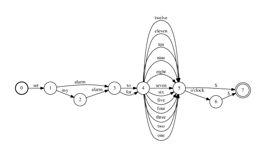
Figure 1: An unweighted automaton that specifies what one might say to set an alarm. The initial state is the bold circle and the final state is the double circle. By convention, we terminate all accepted strings with the symbol $\$\,$.

As stated earlier, some applications may simply require smaller models or those with lower latency of inference, and in such scenarios the specific target topology may be unknown. In such cases, one choice is to build a $k$-gram deterministic finite automaton (DFA) topology from a corpus drawn from $S$ [5]. This could be from an existing corpus or from random samples drawn from $S$. Figure 2a shows a trigram topology for the very simple corpus $aab$. Figure 2b shows an alternative topology that allows skip-grams. Both of these representations make use of failure transitions. These allow modeling strings unseen in the corpus (e.g., $abab$) in a compact way by failing or backing-off to states that correspond to lower-order histories. Such models can be made more elaborate if some transitions represent classes, such as names or numbers, that are themselves represented by sub-automata. As mentioned previously, we will mostly assume we have a topology either pre-specified or inferred by some means and focus on how to weight that topology to best approximate the source distribution. We hence focus our evaluation on intrinsic measures of model quality such as perplexity or bits-per-character.

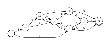
(a)

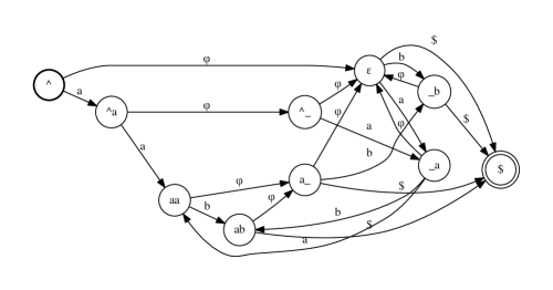
(b)

Figure 2: Topology examples derived from the corpus $aab$. States are labeled with the context that is remembered, $\wedge\,$denotes the initial context, $\epsilon$ the empty context, $\$\,$the final context (and terminates accepted strings), and $\_$ matches any symbol in a context. (a) $3$-gram topology: failure transitions, labeled with $\varphi$, implement backoff from histories $xy$ to $\_y$ to $\epsilon$. (b) skip-gram topology: failure transitions implement backoff instead from histories $xy$ to $x\_$.

This paper expands upon an earlier, shorter version [56] by also providing, beyond the additional motivating examples that have already been presented in this introduction: an extended related work section and references; expansion of the theoretical analysis from three lemmas without proofs (omitted for space) to five lemmas (and a corollary) with full proofs; inclusion of additional algorithms for counting (for general WFA source and target in addition to $\varphi$-WFA); inclusion of additional experiments, including some illustrating the exact KL-minimization methods available for WFA sources of different classes; and documentation of the open-source library that provides the full functionality presented here.

The paper is organized as follows. In Section 2 we review previous work in this area. In Section 3 we give the theoretical formulation of the problem and the minimum KL divergence approximation. In Section 4 we present algorithms to compute that solution. One algorithm is for the case that the source itself is finite-state. A second algorithm is for the case when it is not and involves a sampling approach. In Section 5 we show experiments using the approximation. In Section 6 we briefly describe the open-source software used in our experiments. Finally, in Section 7 we discuss the results and offer conclusions.

2 Related work

In this section we will review methods both for inferring unweighted finite-state models from data and estimating the weight distribution as well in the weighted case. We start with the unweighted case.

There is a long history of unweighted finite-state model inference [49, 19]. Gold [28] showed that an arbitrary regular set $L$ cannot be learned, identified in the limit, strictly from the presentation of a sequence of positive examples that eventually includes each string in $L$. This has led to several alternative lines of attack.

One approach is to include the negative examples in the sequence. Given such a complete sample, there are polynomial-time algorithms that identify a regular set in the limit [29]. For example, a prefix tree of the positive examples can be built and then states can be merged so long as they do not cause a negative example to be accepted [47, 23]. Another approach is to train a recurrent neural network (RNN) on the positive and negative examples and then extract a finite automaton by quantizing the continuous state space of the RNN [27, 34].

A second approach is to assume a teacher is available that determines not only if a string is a positive or negative example but also if the language of the current hypothesized automaton equals $L$ or, if not, provides a counterexample. In this case the minimal $m$-state DFA corresponding to $L$ can be learned in time polynomial in $m$ [7]. Weiss et al. [58] apply this method for DFA extraction from an RNN.

A third approach is to assume a probability distribution over the (positive only) samples. With some reasonable restrictions on the distribution, such as that the probabilities are generated from a weighted automaton $A$ with $L={\cal L}(A)$, then $L$ is identifiable in the limit with ‘high probability’ [8, 50].

There have been a variety of approaches for estimating weighted automata. A variant of the prefix tree construction can be used that merges states with sufficiently similar suffix distributions, estimated from source frequencies [14, 15]. Approaches that produce (possibly highly) non-deterministic results include the Expectation-Maximization (EM) algorithm [21] applied to a fully connected Hidden Markov models or spectral methods applied to automata [10, 11]. Eisner [26] describes an algorithm for estimating probabilities in a finite-state transducer from data using EM-based methods. Weiss et al. [59] and Okudono et al. [46] provide adaptations to the Weiss et al. [58] DFA extraction algorithm to yield weighted automata.

For approximating neural network (NN) models as WFAs, Deoras et al. [22] used an RNN LM to generate samples that they then used to train a $k$-gram LM. Arisoy et al. [9] used deep neural network (DNN) models of different orders to successively build and prune a $k$-gram LM with each new order constrained by the previous order. Adel et al. [1] also trained DNNs of different orders, built a $k$-gram LM on the same data to obtain a topology and then transferred the DNN probabilities of each order onto that $k$-gram topology. Tiño and Vojtek [57] quantized the continuous state space of an RNN and then estimated the transition probabilities from the RNN. Lecorvé and Motlicek [38] quantized the hidden states in an LSTM to form a finite-state model and then used an entropy criterion to backoff to low-order $k$-grams to limit the number of transitions. See Section 4.3 for a more detailed comparison with the most closely related methods, once the details of our algorithms have been provided.

Our paper is distinguished in several respects from previous work. First, our general approach does not depend on the form the source distribution although we specialize our algorithms for (known) finite-state sources with an efficient direct construction and for other sources with an efficient sampling approach. Second, our targets are a wide class of deterministic automata with failure transitions. These are considerably more general than $k$-gram models but retain the efficiency of determinism and the compactness failure transitions allow, which is especially important in applications with large alphabets like language modeling. Third, we show that our approximation searches for the minimal KL divergence between the source and target distributions, given a fixed target topology provided by the application or some earlier computation.

3 Theoretical analysis

3.1 Probabilistic models

Let $\Sigma$ be a finite alphabet. Let $x^{n}_{i}\in\Sigma^{*}$ denote the string $x_{i}x_{i+1}\ldots x_{n}$ and $x^{n}\triangleq x^{n}_{1}$. A probabilistic model $p$ over $\Sigma$ is a probabilistic distribution over the next symbol $x_{n}$, given the previous symbols $x^{n-1}$, such that

$$\sum_{x\in\Sigma}p(x_{n}=x|x^{n-1})=1\text{ and }p(x_{n}=x|x^{n-1})\geq 0,\forall x\in\Sigma.$$

Without loss of generality, we assume that the model maintains an internal state $q$ and updates it after observing the next symbol. Furthermore, the probability of the subsequent state just depends on the state $q$

$$p(x^{n}_{i+1}|x^{i})=p(x^{n}_{i+1}|q(x^{i})),$$

for all $i,n,x^{i},x^{n}_{i+1}$, where $q(x^{i})$ is the state that the model has reached after observing sequence $x^{i}$. Let $Q(p)$ be the set of possible states. Let the language $\mathcal{L}(p)\subseteq\Sigma^{*}$ defined by the distribution $p$ be

$$\mathcal{L}(p)\triangleq\{x^{n}\in\Sigma^{*}:p(x^{n})>0\text{ and }x_{n}=\text{$\$\,$}\text{ and }x_{i}\neq\text{$\$\,$},\forall\ i<n\}.$$ (2)

The symbol $\$\,$ is used as a stopping criterion. Further for all $x^{n}\in\Sigma^{*}$ such that $x_{n-1}=\text{$\$\,$}$, $p(x_{n}|x^{n-1})=0$.

The KL divergence between the source model $p_{s}$ and the target model $p_{a}$ is given by

$$D(p_{s}||p_{a})=\sum_{x^{n}\in\Sigma^{*}}p_{s}(x^{n})\log\frac{p_{s}(x^{n})}{p_{a}(x^{n})},$$ (3)

where for notational simplicity, we adopt the notion $0/0=1$ and $0\log(0/0)=0$ throughout the paper. Note that for the KL divergence to be finite, we need $\mathcal{L}(p_{s})\subseteq\mathcal{L}(p_{a})$. We will assume throughout the source entropy $H(p_{s})=-\sum_{x^{n}}p_{s}(x^{n})\log p_{s}(x^{n})$ is finite. We first reduce the KL divergence between two models as follows [cf. 13, 20]. In the following, let $q_{*}$ denote the states of the probability distribution $p_{*}$.

Lemma 1.

If $\mathcal{L}(p_{s})\subseteq\mathcal{L}(p_{a})$, then

$$D(p_{s}||p_{a})=\sum_{q_{a}\in Q_{a}}\sum_{q_{s}\in Q_{s}}\sum_{x\in\Sigma}\gamma(q_{s},q_{a})\,p_{s}(x|q_{s})\log\frac{p_{s}(x|q_{s})}{p_{a}(x|q_{a})},$$ (4)

where

$$\gamma(q_{s},q_{a})=\sum^{\infty}_{i=0}\sum_{x^{i}:q_{s}(x^{i})=q_{s},q_{a}(x^{i})=q_{a}}p_{s}(x^{i}).$$ (5)

Proof.

$$D(p_{s}||p_{a}) =\sum^{\infty}_{n=1}\sum_{x^{n}}p_{s}(x^{n})\log\frac{p_{s}(x^{n})}{p_{a}(x^{n})}$$

$$=\sum^{\infty}_{n=1}\sum_{x^{n}}p_{s}(x^{n})\sum^{n}_{i=1}\log\frac{p_{s}(x_{i}|x^{i-1})}{p_{a}(x_{i}|x^{i-1})}$$

$$=\sum^{\infty}_{n=1}\sum^{n}_{i=1}\sum_{x^{n}}p_{s}(x^{n})\log\frac{p_{s}(x_{i}|x^{i-1})}{p_{a}(x_{i}|x^{i-1})}$$

$$=\sum^{\infty}_{n=1}\sum^{n}_{i=1}\sum_{x^{n}}p_{s}(x^{i-1})p_{s}(x_{i}|x^{i-1})p_{s}(x^{n}_{i+1}|x^{i})\log\frac{p_{s}(x_{i}|x^{i-1})}{p_{a}(x_{i}|x^{i-1})}$$

$$=\sum^{\infty}_{i=1}\sum_{x^{i-1}}p_{s}(x^{i-1})\sum_{x_{i}}p_{s}(x_{i}|x^{i-1})\log\frac{p_{s}(x_{i}|x^{i-1})}{p_{a}(x_{i}|x^{i-1})}\cdot\sum_{n\geq i}\sum_{x^{n}_{i+1}}p_{s}(x^{n}_{i+1}|x^{i})$$

$$=\sum^{\infty}_{i=1}\sum_{x^{i-1}}p_{s}(x^{i-1})\sum_{x_{i}}p_{s}(x_{i}|x^{i-1})\log\frac{p_{s}(x_{i}|x^{i-1})}{p_{a}(x_{i}|x^{i-1})}.$$

By definition, the probability of the next symbol conditioned on the past just depends on the state. Hence grouping terms corresponding to same states both in $s$ and $t$ yields,

$$\sum^{\infty}_{i=1}\sum_{x^{i-1}}p_{s}(x^{i-1})\sum_{x_{i}}p_{s}(x_{i}|x^{i-1})\log\frac{p_{s}(x_{i}|x^{i-1})}{p_{a}(x_{i}|x^{i-1})}$$

$$=\sum^{\infty}_{i=1}\sum_{x^{i-1}}p_{s}(x^{i-1})\sum_{x_{i}}p_{s}(x_{i}|q_{s}(x^{i-1}))\log\frac{p_{s}(x_{i}|q_{s}(x^{i-1}))}{p_{a}(x_{i}|q_{a}(x^{i-1}))}$$

$$=\sum_{q_{a}\in Q_{a}}\sum_{q_{s}\in Q_{s}}\sum^{\infty}_{i=1}\sum_{x^{i-1}:q_{s}(x^{i-1})=q_{s},q_{a}(x^{i-1})=q_{a}}p_{s}(x^{i-1})\sum_{x_{i}}p_{s}(x_{i}|q_{s})\log\frac{p_{s}(x_{i}|q_{s})}{p_{a}(x_{i}|q_{a})}$$

$$=\sum_{q_{a}\in Q_{a}}\sum_{q_{s}\in Q_{s}}\sum_{x_{i}}\gamma(q_{s},q_{a})\,p_{s}(x_{i}|q_{s})\log\frac{p_{s}(x_{i}|q_{s})}{p_{a}(x_{i}|q_{a})}.$$

Replacing $x_{i}$ by $x$ yields the lemma. ∎

The quantity $\gamma(q_{s},q_{a})$ counts each string $x^{i}$ that reaches both state $q_{s}$ in $Q_{s}$ and state $q_{a}$ in $Q_{a}$ weighted by its probability according to $p_{s}$. Equivalently it counts each string $x^{i}$ reaching state $(q_{s},q_{a})$ in $Q_{s}\times Q_{a}$ (an interpretation we develop in Section 4.1.1). Note $\gamma$ does not depend on distribution $p_{a}$.

The following corollary is useful for finding the probabilistic model $p_{a}$ that has the minimal KL divergence from a model $p_{s}$.

Corollary 1.

Let $\mathscr{P}$ be a set of probabilistic models $p_{a}$ for which $\mathcal{L}(p_{s})\subseteq\mathcal{L}(p_{a})$. Then

$$\mathop{\rm argmin}\limits_{p_{a}\in\mathscr{P}}D(p_{s}||p_{a})\\ =\mathop{\rm argmax}\limits_{p_{a}\in\mathscr{P}}\sum_{q_{a}\in Q_{a}}\sum_{x\in\Sigma}c(x,q_{a})\log p_{a}(x|q_{a}),$$

where

$$c(x,q_{a})=\sum_{q_{s}\in Q_{s}}\gamma(q_{s},q_{a})\,p_{s}(x|q_{s}).$$ (6)

Proof.

By Lemma 5

$$\mathop{\rm argmin}\limits_{p_{a}\in\mathscr{P}}D(p_{s}||p_{a})= \mathop{\rm argmin}\limits_{p_{a}\in\mathscr{P}}\sum_{q_{a}\in Q_{a}}\sum_{q_{s}\in Q_{s}}\sum_{x\in\Sigma}\gamma(q_{s},q_{a})\,p_{s}(x|q_{s})\log\frac{p_{s}(x|q_{s})}{p_{a}(x|q_{a})}$$

$$= \mathop{\rm argmin}\limits_{p_{a}\in\mathscr{P}}\Big{\{}\sum_{q_{a}\in Q_{a}}\sum_{q_{s}\in Q_{s}}\sum_{x\in\Sigma}\gamma(q_{s},q_{a})\,p_{s}(x|q_{s})\log p_{s}(x|q_{s})$$

$$\qquad\quad-\sum_{q_{a}\in Q_{a}}\sum_{q_{s}\in Q_{s}}\sum_{x\in\Sigma}\gamma(q_{s},q_{a})\,p_{s}(x|q_{s})\log{p_{a}(x|q_{a})}\Big{\}}$$ (7)

$$= \mathop{\rm argmax}\limits_{p_{a}\in\mathscr{P}}\sum_{q_{a}\in Q_{a}}\sum_{x\in\Sigma}c(x,q_{a})\log p_{a}(x|q_{a}),$$

since the first term in Equation 7 does not depend on $p_{a}$. ∎

The quantity $c(x_{i},q_{a})$ counts each string $x^{i}$ that reaches a state $(q_{s},q_{a})$ in $Q_{s}\times\{q_{a}\}$ by $x_{1}^{i-1}$ weighted by its probability according to $p_{s}$ (cf. Equation 18).

3.2 Weighted finite automata

A weighted finite automaton $A=(\Sigma,Q,E,i,f)$ over $\mathbb{R}_{+}$ is given by a finite alphabet $\Sigma$, a finite set of states $Q$, a finite set of transitions $E\subseteq Q\times\Sigma\times\mathbb{R}_{+}\times Q$, an initial state $i\in Q$ and a final state $f\in Q$. A transition $e=(p[{e}],\ell[e],w[e],n[{e}])\in E$ represents a move from a previous (or source) state $p[{e}]$ to the next (or destination) state $n[{e}]$ with the label $\ell[e]$ and weight $w[e]$. The transitions with previous state $q$ are denoted by $E[q]$ and the labels of those transitions as $L[q]$.

A deterministic WFA has at most one transition with a given label leaving each state. An unweighted (finite) automaton is a WFA that satisfies $w[e]=1,\forall e\in E$. A probabilistic (or stochastic) WFA satisfies

$$\sum_{e\in E[q]}w[e]=1\text{ and }w[e]\geq 0,\quad\forall q\in Q-\{f\}.$$

Transitions $e_{1}$ and $e_{2}$ are consecutive if $n[{e_{i}}]=p[{e_{i+1}}]$. A path $\pi=e_{1}\cdots e_{n}\in E^{*}$ is a finite sequence of consecutive transitions. The previous state of a path we denote by $p[{\pi}]$ and the next state by $n[{\pi}]$. The label of a path is the concatenation of its transition labels $\ell[\pi]=\ell[e_{1}]\cdots\ell[e_{n}]$. The weight of a path is obtained by multiplying its transition weights $w[\pi]=w[e_{1}]\times\cdots\times w[e_{n}]$. For a non-empty path, the $i$-th transition is denoted by $\pi_{i}$.

$P(q,q^{\prime})$ denotes the set of all paths in $A$ from state $q$ to $q^{\prime}$. We extend this to sets in the obvious way: $P(q,R)$ denotes the set of all paths from state $q$ to $q^{\prime}\in R$ and so forth. A path $\pi$ is successful if it is in $P(i,f)$ and in that case the automaton is said to accept the input string $\alpha=\ell[\pi]$.

The language accepted by an automaton $A$ is the regular set $\mathcal{L}(A)=\{\alpha\in\Sigma^{*}:\alpha=\ell[\pi],\pi\in P(i,f)\}$. The weight of $\alpha\in\mathcal{L}(A)$ assigned by the automaton is $A(\alpha)=\Sigma_{\pi\in P(i,f):\,\ell[\pi]=\alpha}w[\pi]$. Similar to Equation 2, we assume a symbol $\text{$\$\,$}\in\Sigma$ such that

$$\mathcal{L}(A)\subseteq\{x^{n}\in\Sigma^{*}:x_{n}=\text{$\$\,$}\text{ and }x_{i}\neq\text{$\$\,$},\forall\ i<n\}.$$

Thus all successful paths are terminated by the symbol $\$\,$.

For a symbol $x\in\Sigma$ and a state $q\in Q$ of a deterministic, probabilistic WFA A, define a distribution $p_{a}(x|q)\triangleq w\text{ if }(q,x,w,q^{\prime})\in E$ and $p_{a}(x|q)\triangleq 0$ otherwise. Then $p_{a}$ is a probabilistic model over $\Sigma$ as defined in the previous section. If $A=(\Sigma,Q,E,i,f)$ is an unweighted deterministic automaton, we denote by $\mathscr{P}(A)$ the set of all probabilistic models $p_{a}$ representable as a weighted WFA $\hat{A}=(\Sigma,Q,\hat{E},i,f)$ with the same topology as $A$ where $\hat{E}=\{(q,x,p_{a}(x|q),q^{\prime}):(q,x,1,q^{\prime})\in E\}$.

Given an unweighted deterministic automaton $A$, our goal is to find the target distribution $p_{a}\in\mathscr{P}(A)$ that has the minimum KL divergence from our source probability model $p_{s}$.

Lemma 2.

If $\mathcal{L}(p_{s})\subseteq\mathcal{L}(A)$, then

$$\mathop{\rm argmin}\limits_{p_{a}\in\mathscr{P}(A)}D(p_{s}||p_{a})=\tilde{p}(x|q_{a})\triangleq\frac{c(x,q_{a})}{c(q_{a})},$$ (8)

where

$$c(q_{a})=\sum_{x\in\Sigma}c(x,q_{a}).$$

Proof.

From Corollary 6

$$\mathop{\rm argmin}\limits_{p_{a}\in\mathscr{P}(A)}D(p_{s}||p_{a}) =\mathop{\rm argmax}\limits_{p_{a}\in\mathscr{P}(A)}\sum_{q_{a}\in Q_{a}}\sum_{x\in\Sigma}c(x,q_{a})\log p_{a}(x|q_{a})$$

$$=\mathop{\rm argmax}\limits_{p_{a}\in\mathscr{P}(A)}\sum_{q_{a}\in Q_{a}}\sum_{x\in\Sigma}c(q_{a})\,\tilde{p}(x|q_{a})\log p_{a}(x|q_{a})$$

$$=\mathop{\rm argmin}\limits_{p_{a}\in\mathscr{P}(A)}\sum_{q_{a}\in Q_{a}}c(q_{a})\Big{\{}-\sum_{x\in\Sigma}\tilde{p}(x|q_{a})\log p_{a}(x|q_{a})\Big{\}}.$$

The quantity in braces is minimized when $p_{a}(x|q_{a})=\tilde{p}(x|q_{a})$ since it is the cross entropy between the two distributions. Since $\mathcal{L}(p_{s})\subseteq\mathcal{L}(A)$, it follows that $\tilde{p}\in\mathscr{P}(A)$. ∎

3.3 Weighted finite automata with failure transitions

A weighted finite automaton with failure transitions ($\varphi$-WFA) $A=(\Sigma,Q,E,i,f)$ is a WFA extended to allow a transition to have a special failure label denoted by $\varphi$. Then $E\subseteq Q\times(\Sigma\cup\{\varphi\})\times\mathbb{R}_{+}\times Q$.

A $\varphi$ transition does not add to a path label; it consumes no input.. However it is followed only when the input cannot be read immediately. Specifically, a path $e_{1}\cdots e_{n}$ in a $\varphi$-WFA is disallowed if it contains a subpath $e_{i}\cdots e_{j}$ such that $\ell[e_{k}]=\varphi$ for all $k$, $i\leq k<j$, and there is another transition $e\in E$ such that $p[{e_{i}}]=p[{e}]$ and $\ell[e_{j}]=\ell[e]\in\Sigma$ (see Figure 3). Since the label $x=l[e_{j}]$ can be read on $e$, we do not follow the failure transitions to read it on $e_{j}$ as well.

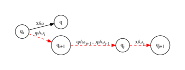
Figure 3: The (dashed red) path $e_{i}=(q_{i},\varphi,\omega_{i},q_{i+1})$ to $e_{j}=(q_{j},x,\omega_{j},q_{j+1})$ is disallowed since $x$ can be read already on $e=(q_{i},x,\omega,q)$.

We use $P^{*}(q,q^{\prime})\subseteq P(q,q^{\prime})$ to denote the set of (not dis-) allowed paths from state $q$ to $q^{\prime}$ in a $\varphi$-WFA. This again extends to sets in the obvious way. A path $\pi$ is successful in a $\varphi$-WFA if $\pi\in P^{*}(i,f)$ and only in that case is the input string $\alpha=\ell[\pi]$ accepted.

The language accepted by the $\varphi$-automaton $A$ is the set $\mathcal{L}(A)=\{\alpha\in\Sigma^{*}:\alpha=\ell[\pi],\pi\in P^{*}(i,f)\}$. The weight of $\alpha\in\Sigma^{*}$ assigned by the automaton is $A{(\alpha)}=\Sigma_{\pi\in P^{*}(i,f):\,\ell[\pi]=\alpha}w[\pi]$. We assume each string in $\mathcal{L}(A)$ is terminated by the symbol $\$\,$ as before. We also assume there are no $\varphi$-labeled cycles and there is at most one exiting failure transition per state.

We express the $\varphi$-extended transitions leaving $q$ as

$$\ E^{*}[q]=\Big{\{}(q,x,\omega,q^{\prime}):\quad \pi\in P^{*}(q,Q),x=\ell[\pi]=\ell[\pi_{|\pi|}]\in\Sigma,\omega=w[\pi],q^{\prime}=n[{\pi}]\Big{\}}.$$

This is a set of (possibly new) transitions $(q,x,\omega,q^{\prime})$, one for each allowed path from previous state $q$ to next state $q^{\prime}$ with optional leading failure transitions and a final $x$-labeled transition. Denote the labels of $E^{*}[q]$ by $L^{*}[q]$. Note the WFA $(\Sigma,Q,E^{*},i,f)$ accepts the same strings with the same weights as $\varphi$-WFA $A$ and thus $\mathcal{L}(A)$ is regular [4].

A probabilistic (or stochastic) $\varphi$-WFA satisfies

$$\sum_{e\in E^{*}[q]}w[e]=1\text{ and }w[e]\geq 0,\quad\forall q\in Q-\{f\}.$$

A deterministic $\varphi$-WFA is backoff-complete if a failure transition from state $q$ to $q^{\prime}$ implies $L[q]\cap\Sigma\subseteq L[q^{\prime}]\cap\Sigma$. Further, if $\varphi\notin L[q^{\prime}]$, then the containment is strict: $L[q]\cap\Sigma\subset L[q^{\prime}]\cap\Sigma$. In other words, if a symbol can be read immediately from a state $q$ it can also be read from a state failing (backing-off) from $q$ and if $q^{\prime}$ does not have a backoff arc, then at least one additional label can be read from $q^{\prime}$ that cannot be read from $q$. For example, both topologies depicted in Figure 2 have this property. We restrict our target automata to have a topology with the backoff-complete property since it will simplify our analysis, make our algorithms efficient and is commonly found in applications. For example backoff $n$-gram models, such the Katz model, are $\varphi$-cycle-free, backoff-complete $\varphi$-WFAs [35, 18].

For a symbol $x\in\Sigma$ and a state $q\in Q$ of a deterministic, probabilistic $\varphi$-WFA A, define $p^{*}_{a}(x|q)\triangleq w\text{ if }(q,x,w,q^{\prime})\in E^{*}[q]$ and $p^{*}_{a}(x|q)\triangleq 0$ otherwise. Then $p^{*}_{a}$ is a probabilistic model over $\Sigma$ as defined in Section 3.1. Note the distribution $p^{*}_{a}$ at a state $q$ is defined over the $\varphi-$extended transitions $E^{*}[q]$ where $p_{a}$ in the previous section is defined over the transitions $E[q]$. It is convenient to define a companion distribution $p_{a}\in\mathscr{P}(A)$ to $p_{a}^{*}$ as follows: given a symbol $x\in\Sigma\cup\{\varphi\}$ and state $q\in Q$, define $p_{a}(x|q)\triangleq p^{*}_{a}(x|q)$ when $x\in L[q]\cap\Sigma$, $p_{a}(\varphi|q)\triangleq 1-\sum_{x\in L[q]\cap\Sigma}p^{*}_{a}(x|q)$, and $p_{a}(x|q)\triangleq 0$ otherwise. The companion distribution is thus defined solely over the transitions $E[q]$.

When $A=(\Sigma,Q,E,i,f)$ is an unweighted deterministic, backoff-complete $\varphi$-WFA, we denote by $\mathscr{P}^{*}(A)$ the set of all probabilistic models $p^{*}_{a}$ representable as a weighted $\varphi$-WFA $\hat{A}=(\Sigma,Q,\hat{E},i,f)$ of same topology as $A$ with

$$\hat{E}= \{(q,x,p_{a}(x|q),q^{\prime}):(q,x,1,q^{\prime})\in E,x\in\Sigma\}\,\cup$$

$$\{(q,\varphi,\alpha(q,q^{\prime}),q^{\prime}):(q,\varphi,1,q^{\prime})\in E\},$$

where $p_{a}\in\mathscr{P}(A)$ is the companion distribution to $p_{a}^{*}$ and $\alpha(q,q^{\prime})=p_{a}(\varphi|q)/d(q,q^{\prime})$ is the weight of the failure transition from state $q$ to $q^{\prime}$ with

$$d(q,q^{\prime})=1-\sum_{x\in L[q]\cap\Sigma}p_{a}(x|q^{\prime}).$$ (9)

Note we have specified the weights on the automaton that represents $p_{a}^{*}\in\mathscr{P}^{*}(A)$ entirely in terms of the companion distribution $p_{a}\in\mathscr{P}(A)$. The failure transition weight $\alpha$ is determined from the requirement that $\sum_{x}E^{*}[q]=1$ [35, Equation 16]. Thanks to the backoff-complete property, this transition weight depends only on its previous state $q$ and its next state $q^{\prime}$ and not all the states in the failure path from $q$. This is a key reason for assuming that property; otherwise our algorithms could not benefit from this locality.

Conversely, each distribution $p_{a}\in\mathscr{P}(A)$ can be associated to a distribution $p^{*}_{a}\in\mathscr{P}^{*}(A)$ given a deterministic, backoff-complete $\varphi$-WFA $A$. First extend $\alpha(q,q^{\prime})$ to any failure path as follows. Denote a failure path from state $q$ to $q^{\prime}$ by $\pi_{\varphi}(q,q^{\prime})$. Then define

$$\alpha(q,q^{\prime})=\prod_{e\in\pi_{\varphi}(q,q^{\prime})}\frac{p_{a}(\varphi|p[{e}])}{d(p[{e}],n[{e}])},$$ (10)

where this quantity is taken to be $1$ when the failure path is empty ($q=q^{\prime}$). Finally define

$$p^{*}_{a}(x|q)=\begin{cases}\alpha(q,q^{x})\,p_{a}(x|q^{x}),&x\in L^{*}[q]\\ 0,&\text{otherwise}\end{cases}$$ (11)

where for $x\in L^{*}[q]$, $q^{x}$ signifies the first state $q^{\prime}$ on a $\varphi$-labeled path in $A$ from state $q$ for which $x\in L[q^{\prime}]$.

For (10) to be well-defined, we need $d(p[{e}],n[{e}])>0$. To ensure this condition, we restrict $\mathscr{P}(A)$ to contain distributions such that $p_{a}(x|q)\geq\epsilon$ for each $x\in L[q]$.

Given an unweighted deterministic, backoff-complete, automaton $A$, our goal is to find the target distribution $p^{*}_{a}\in\mathscr{P}^{*}(A)$ that has the minimum KL divergence from our source probability model $p_{s}$.

Lemma 3.

Assume $\mathcal{L}(p_{s})\subseteq\mathcal{L}(A)$. Let $p^{*}=\tilde{p}(x|q_{a})$ from Lemma 2. If $\mathcal{L}(p^{*})\subseteq\mathcal{L}(A)$ and $p^{*}\in\mathscr{P}^{*}(A)$ then

$$p^{*}=\mathop{\rm argmin}\limits_{p^{*}_{a}\in\mathscr{P}^{*}(A)}D(p_{s}||p^{*}_{a}).$$

Proof.

This follows immediately from Lemma 2. ∎

The requirement that the $p^{*}$ of Lemma 3 is in $\mathscr{P}^{*}(A)$ will be true if, for instance, the target has no failure transitions or if the source and target are both $\varphi$-WFAs with the same topology and failure transitions. In general, this requirement can not be assured. While membership in $\mathscr{P}(A)$ principally requires the weights of the transitions leaving a state are non-negative and sum to $1$, membership in $\mathscr{P}^{*}(A)$ imposes additional constraints due to the failure transitions, indicated in Equation 11.

As such, we restate our goal in terms of the companion distribution $p_{a}\in\mathscr{P}(A)$ rather than its corresponding distribution $p^{*}_{a}\in\mathscr{P}^{*}(A)$ directly. Let $B_{n}(q)$ be the set of states in $A$ that back-off to state $q$ in $n$ failure transitions and let $B(q)=\bigcup^{|Q_{a}|}_{n=0}B_{n}(q)$.

Lemma 4.

If $\mathcal{L}(p_{s})\subseteq\mathcal{L}(A)$ then

$$\mathop{\rm argmin}\limits_{p^{*}_{a}\in\mathscr{P}^{*}(A)}D(p_{s}||p^{*}_{a})=\mathop{\rm argmax}\limits_{p_{a}\in\mathscr{P}(A)}\sum_{q\in Q_{a}}\bigg{\{}\sum_{x\in L[q]}C(x,q)\log p_{a}(x|q)-\sum_{q_{0}\in B_{1}(q)}C(\varphi,q_{0})\log d(q_{0},q)\bigg{\}},$$

where

$$C(x,q) =\sum_{q_{a}\in B(q)}c(x,q_{a})\mathbf{1}_{q=q_{a}^{x}},\quad x\in\Sigma,$$ (12)

$$C(\varphi,q) =\sum_{q_{a}\in B(q)}\sum_{x\in\Sigma}c(x,q_{a})\mathbf{1}_{x\notin L[q]}.$$ (13)

and do not depend on $p_{a}$.

Proof.

From Corollary 6, Equation 11 and the previously shown 1:1 correspondence between each distribution $p^{*}_{a}\in\mathscr{P}^{*}(A)$ and its companion distribution $p_{a}\in\mathscr{P}(A)$

$$\mathop{\rm argmin}\limits_{p^{*}_{a}\in\mathscr{P}^{*}(A)}D(p_{s}||p^{*}_{a}) =\mathop{\rm argmin}\limits_{p^{*}_{a}\in\mathscr{P}^{*}(A)}\sum_{q_{a}\in Q_{a}}\sum_{x\in L^{*}[q_{a}]}c(x,q_{a})\log p^{*}_{a}(x|q_{a})$$

$$=\mathop{\rm argmax}\limits_{p_{a}\in\mathscr{P}(A)}\sum_{q_{a}\in Q_{a}}\sum_{x\in L^{*}[q_{a}]}c(x,q_{a})\log\alpha(q_{a},q^{x}_{a})p_{a}(x|q^{x}_{a})$$

$$=\mathop{\rm argmax}\limits_{p_{a}\in\mathscr{P}(A)}\sum_{q_{a}\in Q_{a}}\sum_{x\in L^{*}[q_{a}]}c(x,q_{a})\log\prod_{e\in\pi_{\varphi}(q_{a},q^{x}_{a})}\frac{p_{a}(\varphi|p[{e}])}{d(p[{e}],n[{e}])}p_{a}(x|q^{x}_{a})$$

$$=\mathop{\rm argmax}\limits_{p_{a}\in\mathscr{P}(A)}\bigg{\{}A_{x}+A_{\varphi}-A_{d}\bigg{\}},$$ (14)

where we distribute the factors inside the logarithm in Equation 14 as follows:

$$A_{x} =\sum_{q_{a}\in Q_{a}}\sum_{x\in L^{*}[q_{a}]}c(x,q_{a})\log p_{a}(x|q^{x}_{a})$$

$$=\sum_{q\in Q_{a}}\sum_{q_{a}\in B(q)}\sum_{x\in L[q]\cap\Sigma}c(x,q_{a})\mathbf{1}_{q=q^{x}_{a}}\log p_{a}(x|q)$$ (15)

$$=\sum_{q\in Q_{a}}\sum_{x\in L[q]\cap\Sigma}C(x,q)\log p_{a}(x|q).$$

Equation 15 follows from $q=q^{x}_{a}$ implying $q_{a}\in B(q)$.

$$A_{\varphi} =\sum_{q_{a}\in Q_{a}}\sum_{x\in L^{*}[q_{a}]}c(x,q_{a})\log\prod_{e\in\pi_{\varphi}(q_{a},q^{x}_{a})}p_{a}(\varphi|p[{e}])$$

$$=\sum_{q_{a}\in Q_{a}}\sum_{x\in L^{*}[q_{a}]}c(x,q_{a})\sum_{e\in\pi_{\varphi}(q_{a},q^{x}_{a})}\log p_{a}(\varphi|p[{e}])$$

$$=\sum_{q\in Q_{a}}\sum_{q_{a}\in B(q)}\sum_{x\in L^{*}[q_{a}]}c(x,q_{a})\sum_{e\in\pi_{\varphi}(q_{a},q^{x}_{a})}\mathbf{1}_{q=p[e]}\log p_{a}(\varphi|q)$$

$$=\sum_{q\in Q_{a}}\sum_{q_{a}\in B(q)}\sum_{x\in\Sigma}c(x,q_{a})\mathbf{1}_{x\notin L[q]}\log p_{a}(\varphi|q)$$ (16)

$$=\sum_{q\in Q_{a}}C(\varphi,q)\log p_{a}(\varphi|q).$$

Equation 16 follows from $e\in\pi_{\varphi}(q_{a},q^{x}_{a})$ implying $x\notin{p[{e}]}$.

$$A_{d} =\sum_{q_{a}\in Q_{a}}\sum_{x\in L^{*}[q_{a}]}c(x,q_{a})\log\prod_{e\in\pi_{\varphi}(q_{a},q^{x}_{a})}d(p[{e}],n[{e}])$$

$$=\sum_{q_{a}\in Q_{a}}\sum_{x\in L^{*}[q_{a}]}c(x,q_{a})\sum_{e\in\pi_{\varphi}(q_{a},q^{x}_{a})}\log d(p[{e}],n[{e}])$$

$$=\sum_{q\in Q_{a}}\sum_{q_{a}\in B(q_{0})}\sum_{q_{0}\in B_{1}(q)}\sum_{x\in L^{*}[q_{a}]}c(x,q_{a})\sum_{e\in\pi_{\varphi}(q_{a},q^{x}_{a})}\mathbf{1}_{q_{0}=p[{e}]}\log d(q_{0},q)$$

$$=\sum_{q\in Q_{a}}\sum_{q_{a}\in B(q_{0})}\sum_{q_{0}\in B_{1}(q)}\sum_{x\in\Sigma}c(x,q_{a})\mathbf{1}_{x\notin L[q_{0}]}\log d(q_{0},q)$$

$$=\sum_{q\in Q_{a}}\sum_{q_{0}\in B_{1}(q)}C(\varphi,q_{0})\log d(q_{0},q).$$

Substituting these results into Equation 14 proves the lemma. ∎

If there are no failure transitions in the target automaton, then $C(x,q)=c(x,q)$, if $x$ is in $\Sigma$, and is $0$ otherwise. In this case, the statement of Lemma 4 simplifies to that of Corollary 6.

Unfortunately, we do not have a closed-form solution, analogous to Lemma 2 or Lemma 3, for the general $\varphi$-WFA case. Instead we will present numerical optimization algorithms to find the KL divergence minimum in the next section. This is aided by the observation that the quantity in braces in the statement of Lemma 4 depends on the distribution $p_{a}$ only at state $q$. Thus the KL divergence minimum can be found by maximizing that quantity independently for each state.

4 Algorithms

Approximating a probabilistic source algorithmically as a weighted finite automaton requires two steps: (1) compute the quantity $c(x,q_{a})$ found in Corollary 6 and Lemma 2 or $C(x,q)$ in Lemma 4 and (2) use this quantity to find the minimum KL divergence solution. The first step, which we will refer to as counting, is covered in the next section and the KL divergence minimization step is covered afterwards, followed by an explicit comparison of the presented algorithms with closely related prior work.

4.1 Counting

How the counts are computed will depend on the form of the source and target models. We break this down into several cases.

4.1.1 WFA source and target

When the source and target models are represented as WFAs we compute $c(x,q_{a})$ from Lemma 2. From Equation 6 this can be written as

$$c(x,q_{a})=\sum_{q_{s}\in Q_{s}}\gamma(q_{s},q_{a})p_{s}(x|q_{s}),$$ (17)

where

$$\gamma(q_{s},q_{a})=\sum^{\infty}_{i=0}\sum_{x^{i}:q_{s}(x^{i})=q_{s},q_{a}(x^{i})=q_{a}}p_{s}(x^{i}).$$

The quantity $\gamma(q_{s},q_{a})$ can be computed as

$$\gamma(q_{s},q_{a})=\sum_{\pi\in P_{S\cap A}((i_{s},i_{a}),(q_{s},q_{a}))}w[\pi],$$

where $S\cap A$ is the weighted finite-state intersection of automata $S$ and $A$ [43]. The above summation over this intersection is the (generalized) shortest distance from the initial state to a specified state computed over the positive real semiring [42, 4]. Algorithms to efficiently compute the intersection and shortest distance on WFAs are available in OpenFst [6], an open-source weighted finite automata library.

Then from Equation 17 we can form the sum

$$c(x,q_{a})=\sum_{((q_{s},q_{a}),x,w,(q_{s}^{\prime},q_{a}^{\prime}))\in E_{S\cap A}}\gamma(q_{s},q_{a})\,w.$$ (18)

Equation 18 is the weighted count of the paths in $S\cap A$ that begin at the initial state and end in any transition leaving a state $(q_{s},q_{a})$ labeled with $x$.

The worst-case time complexity for the counting step is dominated by the shortest distance algorithm on the intersection $S\cap A$. The shortest distance computation is a meta-algorithm that depends on the queue discipline selected [42]. If $s$ is the maximum number of times a state in the intersection is inserted into the shortest distance queue, $C$ the maximum cost of a queue operation, and $D$ the maximum out-degree in $S$ and $A$ (both assumed deterministic), then the algorithm runs in $O(s(D+C)|Q_{S}||Q_{A}|)$ [42, 4]. The worst-case space complexity is in $O(D|Q_{S}||Q_{A}|)$, determined by the intersection size.

4.1.2 $\varphi$-WFA source and target

When the source and target models are represented as $\varphi$-WFAs we compute $C(x,q_{a})$ from Lemma 4. From Equation 12 and the previous case this can be written as

$$C(x,q)=\sum_{q_{a}\in B(q)}\sum_{q_{s}\in Q_{s}}\gamma(q_{s},q_{a})p_{s}(x|q_{s})\mathbf{1}_{q=q_{a}^{x}},\quad x\in\Sigma.$$ (19)

To compute this quantity we first form $S\cap A$ using an efficient $\varphi$-WFA intersection that compactly retains failure transitions in the result as described in [4]. Equation 19 is the weighted count of the paths in $S\cap A$ allowed by the failure transitions that begin at the initial state and end in any transition leaving a state $(q_{s},q)$ labeled with $x$.

We can simplify this computation by the following transformation. First we convert $S\cap A$ to an equivalent WFA by replacing each failure transition with an epsilon transition and introducing a negatively-weighted transition to compensate for formerly disallowed paths [4].

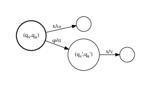
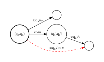
$S\cap A$	$T$

Figure 4: A $\varphi$-WFA is transformed into an equivalent WFA by replacing each failure transition by an $\epsilon$-transition. To compensate for the formerly disallowed paths, new (dashed red) negatively-weighted transitions are added. The result is promoted to a transducer $T$ with the output label used to keep track of the previous state in $A$ of the compensated positive transition.

The result is then promoted to a transducer $T$ with the output label used to keep track of the previous state in $A$ of the compensated positive transition (see Figure 4).. Algorithms to efficiently compute the intersection and shortest distance on $\varphi$-WFAs are available in the OpenGrm libraries [4].

Then

$$C(x,q)=\sum_{((q_{s},q_{a}),x,q,w,(q_{s}^{\prime},q_{a}^{\prime}))\in E_{T}}\gamma_{T}(q_{s},q_{a})w,\quad x\in\Sigma,$$ (20)

where $e=(p[{e}],il[e],ol[e],w[e],n[{e}])$ is a transition in $T$ and $\gamma_{T}(q_{s},q)$ is the shortest distance from the initial state to $(q_{s},q_{a})$ in $T$ computed over the real semiring as described in [4]. Equation 20 is the weighted count of all paths in $S\cap A$ that begin at the initial state and end in any transition leaving a state $(q_{s},q)$ labeled with $x$ minus the weighted count of those paths that are disallowed by the failure transitions.

Finally, we compute $C(\varphi,q)$ as follows. The count mass entering a state $q$ must equal the count mass leaving a state

$$\sum_{(q_{a},x,1,q)\in E_{A}}C(x,q_{a}) =\sum_{(q,x^{\prime},1,q_{a}^{\prime})\in E_{A}}C(x^{\prime},q)$$

$$=\sum_{\begin{subarray}{c}(q,x^{\prime},1,q_{a}^{\prime})\in E_{A},x^{\prime}\in\Sigma\end{subarray}}C(x^{\prime},q)+C(\varphi,q)$$

Thus

$$C(\varphi,q)=\sum_{(q_{a},x,1,q)\in E_{A}}C(x,q_{a})-\sum_{\begin{subarray}{c}(q,x^{\prime},1,q_{a}^{\prime})\in E_{A},x^{\prime}\in\Sigma\end{subarray}}C(x^{\prime},q).$$

This quantity can be computed iteratively in the topological order of states with respect to the $\varphi$-labeled transitions.

The worst-case time and space complexity for the counting step for $\varphi$-WFAs is the same as for WFAs [4].

4.1.3 Arbitrary source and $\varphi$-WFA target

In some cases, the source is a distribution with possibly infinite states, e.g., LSTMs. For these sources, computing $C(x,q)$ can be computationally intractable as (19) requires a summation over all possible states in the source machine, $Q_{s}$. We propose to use a sampling approach to approximate $C(x,q)$ for these cases. Let $x(1),x(2),\ldots,x(N)$ be independent random samples from $p_{s}$. Instead of $C(x,q)$, we propose to use

$$\hat{C}(x,q)=\sum_{q_{a}\in B(q)}\sum_{q_{s}\in Q_{s}}\hat{\gamma}(q_{s},q_{a})p_{s}(x|q_{s})\mathbf{1}_{q=q_{a}^{x}},\quad x\in\Sigma,$$

where

$$\hat{\gamma}(q_{s},q_{a})=\frac{1}{N}\sum^{N}_{j=1}\sum_{i\geq 1}\mathbf{1}_{q_{s}(x^{i}(j))=q_{s},q_{a}(x^{i}(j))=q_{a}}.$$

Observe that in expectation,

$$\mathbb{E}[\hat{\gamma}(q_{s},q_{a})] =\frac{1}{N}\sum^{N}_{j=1}\sum_{i\geq 1}\mathbb{E}[\mathbf{1}_{q_{s}(x^{i}(j))=q_{s},q_{a}(x^{i}(j))=q_{a}}]$$

$$=\sum_{i\geq 1}\sum_{x^{i}:q_{s}(x^{i})=q_{s},q_{a}(x^{i})=q_{a}}p_{s}(x^{i})$$

$$=\gamma(q_{s},q_{a}),$$

and hence $\hat{\gamma}(q_{s},q_{a})$ is an unbiased, asymptotically consistent estimator of $\gamma(q_{s},q_{a})$. Given $\hat{C}(x,q)$, we compute $C(\varphi,q)$ similarly to the previous section. If $\ell$ is the expected number of symbols per sample, then the computational complexity of counting in expectation is in $O(N\ell|\Sigma|)$.

4.2 KL divergence minimization

4.2.1 WFA target

When the target topology is a deterministic WFA, we use $c(x,q_{a})$ from the previous section and Lemma 2 to immediately find the minimum KL divergence solution.

4.2.2 $\varphi$-WFA target

When the target topology is a deterministic, backoff-complete $\varphi$-WFA, Lemma 3 can be applied in some circumstances to find the minimum KL divergence solution but not in general. However, as noted before, the quantity in braces in the statement of Lemma 4 depends on the distribution $p_{a}$ only at state $q$ so the minimum KL divergence $D(p_{s}||p^{*}_{a})$ can be found by maximizing that quantity independently for each state.

Fix a state $q$ and let $y_{x}\triangleq p_{a}(x|q)$ for $x\in L[q]$ and let ${\bf y}\triangleq[y_{x}]_{x\in L[q]}$. Then our goal reduces to

$$\mathop{\rm argmax}\limits_{{\bf y}}\sum_{x\in L[q]}C(x,q)\log y_{x}-\sum_{q_{0}\in B_{1}(q)}C(\varphi,q_{0})\log\big{(}1-\sum_{x\in L[q_{0}]\cap\Sigma}y_{x}\big{)}.$$ (21)

subject to the constraints $y_{x}\geq\epsilon$ for $x\in L[q]$ and $\sum_{x\in L[q]}y_{x}=1$.

This is a difference of two concave functions in ${\bf y}$ since $\log(f({\bf y}))$ is concave for any linear function $f({\bf y})$, $C(x,q),C(\varphi,q_{0})$ are always non-negative and the sum of concave functions is also concave. We give a DC programming solution to this optimization [32]. Let

$$\Omega=\{{\bf y}:\forall x,y_{x}\geq\epsilon,\sum_{x\in L(q)}y_{x}\leq 1\},$$

and let $u({\bf y})=\sum_{x\in L[q]}C(x,q)\log y_{x}$ and $v({\bf y})=\sum_{q_{0}\in B_{1}(q)}C(\varphi,q_{0})\log\big{(}1-\sum_{x\in L[q_{0}]\cap\Sigma}y_{x}\big{)}$. Then the optimization problem can be written as

$$\max_{{\bf y}\in\Omega}u({\bf y})-v({\bf y}).$$

The DC programming solution for such a problem uses an iterative procedure that linearizes the subtrahend in the concave difference about the current estimate and then solves the resulting concave objective for the next estimate [32] i.e.,

$${\bf y}^{n+1}=\mathop{\rm argmax}\limits_{{\bf y}\in\Omega}u({\bf y})-{\bf y}\cdot\triangledown v({\bf y}^{n}).$$

Substituting $u$ and $\triangledown v$ gives

$${\bf y}^{n+1}= \mathop{\rm argmax}\limits_{{\bf y}\in\Omega}\sum_{x\in L[q]}\bigg{\{}C(x,q)\log y_{x}+y_{x}f(x,q,{\bf y}^{n})\bigg{\}},$$ (22)

where

$$f(x,q,{\bf y}^{n})=\sum_{q_{0}\in B_{1}(q)}\frac{C(\varphi,q_{0})\mathbf{1}_{x\in L[q_{0}]\cap\Sigma}}{1-\sum_{x^{\prime}\in L[q_{0}]\cap\Sigma}y_{x^{\prime}}^{n}}.$$ (23)

Observe that ${1-\sum_{x^{\prime}\in L[q_{0}]\cap\Sigma}y_{x^{\prime}}^{n}}\geq\epsilon$ as the automaton is backoff-complete and ${\bf y}^{n}\in\Omega$.

Let $C(q)$ be defined as:

$$C(q)=\sum_{x^{\prime}\in L[q]}C(x^{\prime},q).$$

The following lemma provides the solution to the optimization problem in (22) which leads to a stationary point of the objective.

Lemma 5.

Solution to (22) is given by

$$y^{n+1}_{x}=\max\left(\frac{C(x,q)}{\lambda-f(x,q,{\bf y}^{n})},\epsilon\right),$$ (24)

where $\lambda\in\left[\max_{x\in L[q]}f(x,q,{\bf y}^{n})+C(x,q),\max_{x\in L[q]}f(x,q,{\bf y}^{n})+\frac{C(q)}{1-|L[q]|\epsilon}\right]$ such that $\sum_{x}y^{n+1}_{x}=1$.

Proof.

With KKT multipliers, the optimization problem can be written as

$$\max_{{\bf y},\lambda,\mu_{x}:\mu_{x}\leq 0}\sum_{x\in L[q]}\bigg{\{}C(x,q)\log y_{x}+y_{x}f(x,q,{\bf y}^{n})\bigg{\}}+\lambda\bigl{(}1-\sum_{x\in L[q]}y_{x}\bigr{)}+\sum_{x\in L[q]}\mu_{x}(\epsilon-y_{x}).$$

We divide the proof into two cases depending on the value of $C(x,q)$. Let $C(x,q)\neq 0$. Differentiating the above equation with respect to $y_{x}$ and equating to zero, we get

$$y^{n+1}_{x}=\frac{C(x,q)}{\lambda+\mu_{x}-f(x,q,{\bf y}^{n})}.$$

Furthermore, by the KKT condition, $\mu_{x}(\epsilon-y^{n+1}_{x})=0$. Hence, $\mu_{x}$ is only non-zero if $y^{n+1}_{x}=\epsilon$ and if $\mu_{x}$ is zero, then $y^{n+1}_{x}=\frac{C(x,q)}{\lambda-f(x,q,{\bf y}^{n})}$. Furthermore, since for all $x$, $\mu_{x}\leq 0$, for $y^{n+1}_{x}$ to be positive, we need $\lambda\geq\max_{x}f(x,q,{\bf y}^{n})$. Hence, the above two conditions can be re-expressed as (24). If $C(x,q)=0$, then we get

$$f(x,q,{\bf y}^{n})=\lambda+\mu_{x}\text{ and }\mu_{x}(\epsilon-y^{n+1}_{x})=0,$$

and the solution is given by $y^{n+1}_{x}=\epsilon$ and $\mu_{x}=f(x,q,{\bf y}^{n})-\lambda$. Since $\mu_{x}$ cannot be positive, we have $f(x,q,{\bf y}^{n})\leq\lambda$ for all $x$. Hence, irrespective of the value of $C(x,q)$, the solution is given by (24).

The above analysis restricts $\lambda\geq\max_{x}f(x,q,{\bf y}^{n})$. If $\lambda<f(x,q,{\bf y}^{n})+C(x,q)$, then $y^{n+1}_{x}>1$ and if $\lambda>\max_{x}f(x,q,{\bf y}^{n})+\frac{C(q)}{1-|L[q]|\epsilon}$, then $\sum_{x}y^{n+1}_{x}<1$. Hence $\lambda$ needs to lie in

$$\left[\max_{x\in L[q]}f(x,q,{\bf y}^{n})+C(x,q),\max_{x\in L[q]}f(x,q,{\bf y}^{n})+\frac{C(q)}{1-|L[q]|\epsilon}\right]$$

to ensure that $\sum_{x}y^{n+1}_{x}=1$. ∎

From this, we form the KL-Minimization algorithm in Figure 5. Observe that if all the counts are zero, then for any ${\bf y}$, $u({\bf y})-v({\bf y})=0$ and any solution is an optimal solution and the algorithm returns a uniform distribution over labels. In other cases, we initialize the model based on counts such that ${\bf y}^{0}\in\Omega$. We then repeat the DC programming algorithm iteratively until convergence. Since, $\Omega$ is a convex compact set and functions $u$, $v$, and $\triangledown v$ are continuous and differentiable in $\Omega$, the KL-Minimization converges to a stationary point [53, Theorem $4$]. For each state $q$, the computational complexity of KL-Minimization is in $O(|E[q]|)$ per iteration. Hence, if the maximum number of iterations per each state is $s$, the overall computational complexity of KL-Minimization is in $O(s|E|)$.

Algorithm KL-Minimization Notation:
$\bullet$ $y_{x}=p_{a}(x|q)$ for $x\in L(q)$ $\bullet$ $k=|L[q]|$ $\bullet$ $C(x,q)$ from Equations 12 and 13 $\bullet$ $\textrm{lb}=\max_{x\in L[q]}f(x,q,{\bf y}^{n})+C(x,q)$ $\bullet$ $C(q)=\sum_{x^{\prime}\in L[q]}C(x^{\prime},q)$ $\bullet$ $\textrm{ub}=\max_{x\in L[q]}f(x,q,{\bf y}^{n})+\frac{C(q)}{1-k\epsilon}$ $\bullet$ $f(x,q,{\bf y}^{n})$ from Equation 23 $\bullet$ $\epsilon=$ lower bound on $y_{x}$ Trivial case: If $C(q)=0$, output ${\bf y}$ given by $y_{x}=1/k$ for all $x$. Initialization: Initialize: $$y^{0}_{x}=\frac{C(x,q)}{C(q)}\left(1-k\epsilon\right)+\epsilon.$$ Iteration: Until convergence do: $$y^{n+1}_{x}=\max\left(\frac{C(x,q)}{\lambda-f(x,q,{\bf y}^{n})},\epsilon\right),$$ where $\lambda\in\left[\textrm{lb},\textrm{ub}\right]$ is chosen (in a binary search) to ensure $\sum_{x\in L(q)}y_{x}=1$.

Figure 5: KL-Minimization Algorithm.

4.3 Discussion

Our method for approximating from source $\varphi$-WFAs, specifically from backoff $k$-gram models, shares some similarities with entropy pruning [54]. Both can be used to approximate onto a more compact $k$-gram topology and both use a KL-divergence criterion to do so. They differ in that entropy pruning, by sequentially removing transitions, selects the target topology and in doing so uses a greedy rather than global entropy reduction strategy. We will empirically compare these methods in Section 5.1 for this use case.

Perhaps the closest to our work on approximating arbitrary sources is that of Deoras et al. [22], where they used an RNN LM to generate samples that they then used to train a $k$-gram LM. In contrast, we use samples to approximate the joint state probability $\gamma(q_{s},q_{a})$. If $\ell$ is the average number of words per sentence and $N$ is the total number of sampled sentences, then the time complexity of Deoras et al. [22] is $\mathcal{O}(N\ell|\Sigma|)$ as it takes $\O(|\Sigma|)$ time to generate a sample from the neural model for every word. This is the same as that of our algorithm in Section 4.1.3. However, our approach has several advantages. Firstly, for a given topology, our algorithm provably finds the best KL minimized solution, whereas their approach is optimal only when the size of the $k$-gram model tends to infinity. Secondly, as we show in our experiments, the proposed algorithm performs better compared to that of Deoras et al. [22].

Arisoy et al. [9] and Adel et al. [1] both trained DNN models of different orders as the means to derive probabilities for a $k$-gram model, rather than focusing on model approximation as the above mentioned methods do. Further, the methods are applicable to $k$-gram models specifically, not the larger class of target WFA to which our methods apply.

5 Experiments

We now provide experimental evidence of the theory’s validity and show its usefulness in various applications. For the ease of notation, we use WFA-Approx to denote the exact counting algorithm described in Section 4.1.2 followed by the KL-Minimization algorithm of Section 4.2. Similarly, we use WFA-SampleApprox$($N$)$ to denote the sampled counting described in Section 4.1.3 with $N$ sampled sentences followed by KL-Minimization.

We first give experimental evidence that supports the theory in Section 5.1. We then show how to approximate neural models as WFAs in Section 5.2. We also use the proposed method to provide lower bounds on the perplexity given a target topology in Section 5.3. Finally, we present experiments in Section 5.4 addressing scenarios with source WFAs, hence not requiring sampling. First, motivated by low-memory applications such as (virtual) keyboard decoding [48], we use our approach to create compact language models in Section 5.4.1. Then, in Section 5.4.2, we use our approach to create compact open-vocabulary character language models from count-thresholded $n$-grams.

For most experiments (unless otherwise noted) we use the 1996 CSR Hub4 Language Model data, LDC98T31 (English Broadcast News data). We use the processed form of the corpus and further process it to downcase all the words and remove punctuation. The resulting dataset has $132$M words in the training set, $20$M words in the test set, and has $240$K unique words. For all the experiments that use word models, we create a vocabulary of approximately $32$K words consisting of all words that appeared more than $50$ times in the training corpus. Using this vocabulary, we create a trigram Katz model and prune it to contain $2$M $n$-grams using entropy pruning [54]. We use this pruned model as a baseline in all our word-based experiments. We use Katz smoothing since it is amenable to pruning [16]. The perplexity of this model on the test set is $144.4$. All algorithms were implemented using the open-source OpenFst and OpenGrm $n$-gram and stochastic automata (SFst) libraries with the last library including these implementations [6, 51, 4].

5.1 Empirical evidence of theory

Recall that our goal is to find the distribution on a target DFA topology that minimizes the KL divergence to the source distribution. However, as stated in Section 4.2, if the target topology has failure transitions, the optimization objective is not convex so the stationary point solution may not be the global optimum. We now show that the model indeed converges to a good solution in various cases empirically.

Idempotency

When the target topology is the same as the source topology, we show that the performance of the approximated model matches the source model. Let $p_{s}$ be the pruned Katz word model described above. We approximate $p_{s}$ onto the same topology using WFA-Approx and WFA-SampleApprox$($$\cdot$$)$ and then compute perplexity on the test corpus. The results are presented in Figure 6. The test perplexity of the WFA-Approx model matches that of the source model and the performance of the WFA-SampleApprox$($N$)$ model approaches that of the source model as the number of samples $N$ increases.

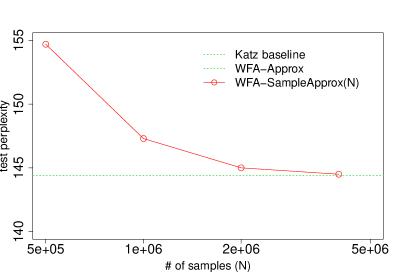
Figure 6: Idempotency: Test set perplexity for Katz baseline and approximations of that baseline trained on the same data. The Katz baseline and Katz WFA-Approx plots are identical (and thus overlap), while WFA-SampleApprox$($N$)$ plot converges to the baseline.

Comparison to greedy pruning

Table 1: Test perplexity of greedy pruning and approximated models.

Model size	Greedy pruning	Approximated model
250K	$205.7$	$198.3$
500K	$177.3$	$173.0$
1M	$157.4$	$155.7$
1.5M	$149.0$	$148.4$

Recall that entropy pruning [54] greedily removes $n$-grams such that the KL divergence to the original model $p_{s}$ is small. Let $p_{\text{greedy}}$ be the resulting model and $A_{\text{greedy}}$ be the topology of $p_{\text{greedy}}$. If the KL-Minimization converges to a good solution, then approximating $p_{s}$ onto $A_{\text{greedy}}$ would give a model that is at least as good as $p_{\text{greedy}}$. We show that this is indeed the case; in fact, approximating $p_{s}$ onto $A_{\text{greedy}}$ performs better than $p_{\text{greedy}}$. As before, let $p_{s}$ again be the $2M$ $n$-gram Katz model described above. We prune it to have $1$M $n$-grams and obtain $p_{\text{greedy}}$, which has a test perplexity of $157.4$. We then approximate the source model $p_{s}$ on $A_{\text{greedy}}$, the topology of $p_{\text{greedy}}$. The resulting model has a test perplexity of $155.7$, which is smaller than the test perplexity of $p_{\text{greedy}}$. This shows that the approximation algorithm indeed finds a good solution. We repeat the experiment with different pruning thresholds and observe that the approximation algorithm provides a good solution across the resulting model sizes. The results are in Table 1.

5.2 Neural models to WFA conversion

Since neural models such as LSTMs give improved performance over $n$-gram models, we investigate whether an LSTM distilled onto a WFA model can obtain better performance than the baseline WFA trained directly from Katz smoothing. As stated in the introduction, this could then be used together with federated learning for fast and private on-device inference, which was done in Chen et al. [17] using the methods presented here.

To explore this, we train an LSTM language model on the training data. The model has $2$ LSTM layers with $1024$ states and an embedding size of $1024$. The resulting model has a test perplexity of $60.5$. We approximate this model as a WFA in three ways.

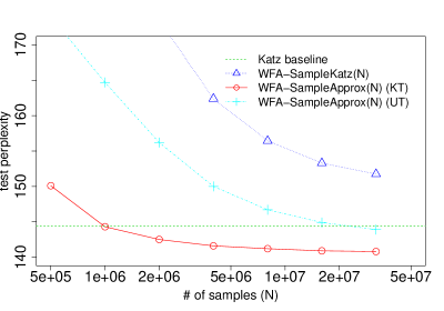
Figure 7: Approximated Neural Models for the English Broadcast News corpus: Test set perplexity for Katz baseline and LSTM models approximated in three ways. One uses LSTM samples to build a new Katz model (WFA-SampleKatz$($N$)$). The remaining two use our approximation algorithm (WFA-SampleApprox$($N$)$), but with different topologies. One topology (KT) is known, using the baseline Katz topology, and one (UT) is unknown, using the samples drawn for WFA-SampleApprox$($N$)$ to also infer the topology.

The first way is to construct a Katz $n$-gram model on $N$ LSTM samples and entropy-prune to $2$M $n$-grams, which we denote by WFA-SampleKatz$($N$)$. This approach is very similar to that of  [22], except that we use Katz smoothing instead of Kneser-Ney smoothing. We used Katz due to the fact that, as stated earlier, Kneser-Ney models are not amenable to pruning [16]. The second way is to approximate onto the baseline Katz $2$M $n$-gram topology described above using WFA-SampleApprox$($N$)$. We refer to this experiment as WFA-SampleApprox$($N$)$ (KT), where KT stands for known topology. The results are shown in Figure 7. The WFA-SampleKatz$($N$)$ models perform significantly worse than the baseline Katz model even at $32$M samples, while the WFA-SampleApprox$($N$)$ models have better perplexity than the baseline Katz model with as little as $1$M samples. With $32$M samples this way of approximating the LSTM model as a WFA is $3.6$ better in perplexity than the baseline Katz.

Finally, if the WFA topology is unknown we use the samples obtained in WFA-SampleApprox$($$\cdot$$)$ to create a Katz model entropy-pruned to $2$M $n$-grams. We refer to this experiment as WFA-SampleApprox$($N$)$ (UT), where UT stands for unknown topology. The results are shown in Figure 7. The approximated models obtained by WFA-SampleApprox$($N$)$ (UT) perform better than WFA-SampleKatz$($N$)$. However, they do not perform as well as WFA-SampleApprox$($N$)$ (KT), the models obtained with the known topology derived from the training data. However, with enough samples, their performance is similar to that of the original Katz model.

We then compare our approximation method with other methods that approximate DNNs with $n$-gram LMs [9, 1]. Both these methods require training DNNs of different orders and we used DNNs with two layers with $1024$ nodes and an embedding size of $1024$. The results are in Table 2. The proposed algorithms WFA-SampleApprox$($$\cdot$$)$ perform better than the existing approaches.

Table 2: Test perplexity of $k$-gram models obtained by different approximation methods for the English Broadcast News corpus. We use 32M samples for both WFA-SampleKatz$($$\cdot$$)$ and WFA-SampleApprox$($$\cdot$$)$.

Model	Test perplexity
Katz	$144.4$
WFA-SampleKatz$($$\cdot$$)$	$151.8$
Arisoy et al. [9]	$159.6$
Adel et al. [1]	$146.7$
WFA-SampleApprox$($$\cdot$$)$ (KT)	$140.8$
WFA-SampleApprox$($$\cdot$$)$ (UT)	$143.9$

Table 3: Test perplexity of $k$-gram models obtained by different approaches for the Polish (Europarl) corpus. We use 32M samples for both WFA-SampleKatz$($$\cdot$$)$ and WFA-SampleApprox$($$\cdot$$)$.

Model	Test perplexity
Katz	$185.5$
WFA-SampleKatz$($$\cdot$$)$	$189.3$
Arisoy et al. [9]	$197.8$
Adel et al. [1]	$187.1$
WFA-SampleApprox$($$\cdot$$)$ (KT)	$181.4$
WFA-SampleApprox$($$\cdot$$)$ (UT)	$177.0$

Experiment on Polish

To repeat the above experiment on a different language and corpus, we turn to the Polish language section of the Europarl corpus [36]. We chose Polish for this follow-up experiment due to the fact that it belongs to a different language family than English, is relatively highly inflected (unlike English) and is found in a publicly available corpus. We use the processed form of the corpus and further process it to downcase all the words and remove punctuation. The resulting dataset has approximately $13$M words in the training set and 210K words in the test set. The selected vocabulary has approximately 30K words, consisting of all words that appeared more than $20$ times in the training corpus. Using this vocabulary, we create a trigram Katz model and prune it to contain $2$M $n$-grams using entropy pruning [54]. We use this pruned model as a baseline. The results are in Figure 8. The trend is similar to that of the English Broadcast News corpus with the proposed algorithm WFA-SampleApprox$($$\cdot$$)$ performing better than the other methods. We also compare the proposed algorithms with other neural approximation algorithms. The comparison results are shown in Table 3.

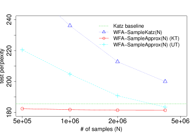
Figure 8: Approximated Neural Models for the Polish (Europarl) corpus: Test set perplexity for Katz baseline and LSTM models approximated in three ways. One uses LSTM samples to build a new Katz model (WFA-SampleKatz$($N$)$). The remaining two use our approximation algorithm (WFA-SampleApprox$($N$)$), but with different topologies. One topology (KT) is known, using the baseline Katz topology, and one (UT) is unknown, using the samples drawn for WFA-SampleApprox$($N$)$ to also infer the topology.

5.3 Lower bounds on perplexity

Best approximation for target topology

The neural model in Section 5.2 has a perplexity of $60.5$, but the best perplexity for the approximated model is $140.8$. Is there a better approximation algorithm for the given target topology? We place bounds on that next.

Let $T$ be the set of test sentences. The test-set log-perplexity of a model $p$ can be written as

$$\frac{1}{|T|}\sum_{x^{*}\in T}\log\frac{1}{p(x^{*})}=\sum_{x^{*}}\hat{p}_{t}(x^{*})\log\frac{1}{p(x^{*})},$$

where $\hat{p}_{t}$ is the empirical distribution of test sentences. Observe that the best model with topology $A$ can be computed as

$$p^{\prime}_{a}=\mathop{\rm argmin}\limits_{p_{a}\in\mathscr{P}(A)}\sum_{x^{*}}\hat{p}_{t}(x^{*})\log\frac{1}{p_{a}(x^{*})},$$

which is the model with topology $A$ that has minimal KL divergence from the test distribution $\hat{p}_{t}$. This can be computed using WFA-Approx. If we use this approach on the English Broadcast News test set with the $2$M $n$-gram Katz model, the resulting model has perplexity of $121.1$, showing that, under the assumption that the algorithm finds the global KL divergence minimum, the test perplexity with this topology cannot be improved beyond $121.1$, irrespective of the method.

Approximation onto best trigram topology

What if we approximate the LSTM onto the best trigram topology, how well does it perform over the test data? To test this, we build a trigram model from the test data and approximate the LSTM on the trigram topology. This approximated model has $11$M $n$-grams and a perplexity of $81$. This shows that for large datasets, the largest shortfall of $n$-gram models in the approximation is due to the $n$-gram topology.

5.4 WFA sources

While distillation of neural models is an important use case for our algorithms, there are other scenarios where approximations will be derived from WFA sources. In such cases, no sampling is required and we can use the algorithms presented in Sections 4.1.1 or 4.1.2, i.e., WFA-Approx. For example, it is not uncommon for applications to place maximum size restrictions on models, so that existing WFA models are too large and must be reduced in size prior to use. Section 5.4.1 presents a couple of experiments focused on character language model size reduction that were motivated by such size restrictions. Another scenario with WFA sources is when, for privacy reasons, no language model training corpus is available in a domain, but only minimum-count-thresholded (i.e., high frequency) word $n$-gram counts are provided. In Section 5.4.2 we examine the estimation of open-vocabulary character language models from such data.

5.4.1 Creating compact language models

Creating compact models for infrequent words

In low-memory applications such as on-device keyboard decoding [48], it is often useful to have a character-level WFA representation of a large set of vocabulary words that act only as unigrams, e.g. those words beyond the $32$K words of our trigram model. We explore how to compactly represent such a unigram-only model.

To demonstrate our approach, we take all the words in the training set (without a count cut-off) and build a character-level deterministic WFA of those words weighted by their unigram probabilities. This is represented as a tree rooted at the initial state (a trie). This automaton has $820$K transitions. Storing this many transitions can be prohibitive; we can reduce the size in two steps.

The first step is to minimize this WFA using weighted minimization [41] to produce $p_{\text{char}}$, which has a topology $A_{\text{char}}$. Although $p_{\text{char}}$ is already much smaller (it has $378$K transitions, a $54\%$ reduction), we can go further by approximating onto the minimal deterministic unweighted automaton, $\text{Minimize}(A_{\text{char}})$. This gives us a model with only $283$K transitions, a further $25\%$ reduction. Since $\text{Minimize}(A_{\text{char}})$ accepts exactly the same words as $A_{\text{char}}$, we are not corrupting our model by adding or removing any vocabulary items. Instead we find an estimate which is as close as possible to the original, but which is constrained to the minimal deterministic representation that preserves the vocabulary.

To evaluate this approach, we randomly select a $20$K sentence subset of the original test set, and represent each selected string as a character-level sequence. We evaluate using cross entropy in bits-per-character, common for character-level models. The resulting cross entropy for $p_{\text{char}}$ is $1.557$ bits-per-character. By comparison, the cross entropy for $p_{\text{char}}$ approximated onto $\text{Minimize}(A_{\text{char}})$ is $1.560$ bits-per-character. In exchange for this small accuracy loss we are rewarded with a model which is $25\%$ smaller. Wolf-Sonkin et al. [60] used the methods presented here to augment the vocabulary of an on-device keyboard to deal with issues related to a lack of standard orthography.

Creating compact WFA language models

Motivated by the previous experiment, we also consider applying (unweighted) minimization to $A_{\text{greedy}}$, the word-based trigram topology that we pruned to $1$M $n$-grams described earlier. In Table 4 we show that applying minimization to $A_{\text{greedy}}$ and then approximating onto the resulting topology leads to a reduction of $7\%$ in the number of transitions needed to represent the model. However, the test perplexity also increases some. To control for this, we prune the original model to a $1.08$M $n$-gram topology $A^{\prime}_{\text{greedy}}$ instead of the $1$M as before and apply the same procedure to obtain an approximation on $\text{Minimize}(A^{\prime}_{\text{greedy}}$). We achieve a $0.4\%$ perplexity reduction compared to the approximation on $A_{\text{greedy}}$ with very nearly the same number of transitions.

Table 4: Test perplexity of models when approximated onto smaller topologies.

Topology	Test perplexity	# Transitions
$A_{\text{greedy}}$	$155.7$	$1.13\text{M}$
$\text{Minimize}(A_{\text{greedy}}$)	$156.4$	$1.05\text{M}$
$A^{\prime}_{\text{greedy}}$	$154.1$	$1.22\text{M}$
$\text{Minimize}(A^{\prime}_{\text{greedy}}$)	$154.9$	$1.13\text{M}$

5.4.2 Count thresholded data for privacy

One increasingly common scenario that can benefit from these algorithms is modeling from frequency thresholded substring counts rather than raw text. For example, word $n$-grams and their frequencies may be provided from certain domains of interest only when they occur within at least $k$ separate documents. With a sufficiently large $k$ (say 50), no $n$-gram can be traced to a specific document, thus providing privacy in the aggregation. This is known as $k$-anonymity [52].

However, for any given domain, there are many kinds of models that one may want to build depending on the task, some of which may be trickier to estimate from such a collection of word $n$-gram counts than with standard approaches for estimation from a given corpus. For example, character $n$-gram models can be of high utility for tasks like language identification, and have the benefit of a relatively small memory footprint and low latency in use. However, character $n$-gram models might be harder to learn from a $k$-anonymized corpus.

Here we will compare open-vocabulary character language models, which accept all strings in $\Sigma^{*}$ for a character vocabulary $\Sigma$, trained in several ways. Each approach relies on the training corpus and 32k vocabulary, with every out-of-vocabulary word replaced by a single OOV symbol $\bigstar$. Additionally, for each approach we add 50 to the unigram character count of any printable ASCII character, so that even those that are unobserved in the words of our 32k vocabulary have some observations. Our three approaches are:

1. Baseline corpus trained models: We count character 5-grams from the $k$-anonymized corpus, then remove all $n$-grams that include the $\bigstar$ symbol (in any position) prior to smoothing and normalization. Here we present both Kneser-Ney and Witten Bell smoothed models, as both are popular for character $n$-gram models.

2. Word trigram sampled model: First we count word trigrams in the $k$-anonymized corpus and discard any $n$-gram with the $\bigstar$ symbol (in any position) prior to smoothing and normalization. We then sample one million strings from a Katz smoothed model and build a character 5-gram model from these strings. We also use this as our target topology for the next approach.

3. Word trigram KL minimization estimation: We create a source model by converting the 2M $n$-gram word trigram model into an open vocabulary model. We do this using a specialized construction related to the construction presented in Section 6 of Chen et al. [17], briefly described below, that converts the word model into a character sequence model. As this model is still closed vocabulary (see below), we additionally smooth the unigram distribution with a character trigram model trained from the words in the symbol table (and including the 50 extra counts for every printable ASCII character as with the other methods). From this source model, we estimate a model on the sampled character 5-gram topology from the previous approach, using our KL minimization algorithm.

Converting word $n$-gram source to character sequence source model

Briefly, for every state $q$ in the $n$-gram automaton, the set of words labeling transitions leaving $q$ are represented as a trie of characters including a final end-of-word symbol. Each resulting transition labeled with the end-of-word symbol represents the last transition for that particular word spelled out by that sequence of transitions, hence is assigned the same next state as the original word transition. If $q$ has a backoff transition pointing to its backoff state $q^{\prime}$, then each new internal state in the character trie backs off to the corresponding state in the character trie leaving $q^{\prime}$. The presence of the corresponding state in the character trie leaving $q^{\prime}$ is guaranteed because the $n$-gram automaton is backoff-complete, as discussed in Section 3.3.

As stated above, this construction converts from word sequences to character sequences, but will only accept character sequences consisting of strings of in-vocabulary words, i.e., this is still closed vocabulary. To make it open vocabulary, we further backoff the character trie leaving the unigram state to a character $n$-gram model estimated from the symbol table (and additional ASCII character observations). This is done using a very similar construction to that described above. The resulting model is used as the source model for our KL minimization algorithm, to estimate a distribution over the sampled character 5-gram topology.

We encode the test set as a sequence of characters, without using the symbol table since our models are intended to be open vocabulary. Following typical practice for open-vocabulary settings, we evaluate with bits-per-character. The results are presented in Table 5. Here we achieve slightly lower bits-per-character than even what we get straight from the corpus, perhaps due to better regularization of the word-based model than with either Witten-Bell or Kneser-Ney on the character n-grams.

Table 5: Comparison of character 5-gram models derived from either the original corpus or a word trigram model. Size of the models is presented in terms of the number of character $n$-grams, the numbers of states and transitions in the automaton representation, and the file size in MB. The two corpus estimated models have the same topology, hence the same size; as do the two word trigram estimated models.

	$n$-grams	states	transitions
Source	(x1000)	(x1000)	(x1000)	MB	Estimation	bits/char
Corpus	336	60	381	6.5	Kneser-Ney	2.04
					Witten-Bell (WB)	2.01
Word trigram	277	56	322	5.6	Sampled (WB)	2.36
					KL min	1.99

6 Software library

All of the algorithms presented here are available in the OpenGrm libraries at http://www.opengrm.org under the topic: SFST Library: operations to normalize, sample, combine, and approximate stochastic finite-state transducers. We illustrate the use of this library by showing how to implement some of the experiments in the previous section.

6.1 Example data and models

Instead of Broadcast News, we will use the text of Oscar Wilde’s The Importance of Being Earnest for our tutorial example. This is a small tutorial corpus that we make available at http://sfst.opengrm.org.

This corpus of approximately 1688 sentences and 18,000-words has been upper-cased and had punctuation removed. The first 850 sentences were used as training data and the remaining 838 sentences used as test data. From these, we produce two 1000-word vocabulary Katz bigram models, the $\sim\!6k$ $n$-gram earnest_train.mod and the $\sim\!4k$ $n$-gram earnest_test.mod. We also used relative-entropy pruning to create the $\sim\!2k$ $n$-gram earnest_train.pru. The data, the steps to generate these models and how to compute their perplexity using OpenGrm NGram are all fully detailed in the QuickTour topic at http://sfst.opengrm.org.

6.2 Computing the approximation

The following step shows how to compute the approximation of a $\varphi$-WFA model onto a $\varphi$-WFA topology. In the example below, the first argument, earnest_train.mod, is the source model, and the second argument, earnest_train.pru, provides the topology. The result is a $\varphi$-WFA whose perplexity can be measured as before.

$ sfstapprox -phi_label=0 earnest_train.mod earnest_train.pru \

>earnest_train.approx

An alternative, equivalent way to perform this approximation is to break it into two steps, with the counting and normalization (KL divergence minimization) done separately.

$ sfstcount -phi_label=0 earnest_train.mod earnest_train.pru \

>earnest_train.approx_cnts

$ sfstnormalize -method=kl_min -phi_label=0 \

earnest_train.approx_cnts >earnest_train.approx

We can now use these utilities to run some experiments analogous to our larger Broadcast News experiments by using different target topologies. The results are shown in Table 6. We see in the idempotency experiment, the perplexity of the approximation on the same topology matches the source. In the greedy-pruning experiment, the approximation onto the greedy-pruned topology yields a better perplexity than the greedily-pruned model. Finally, the approximation onto the test-set bigram topology gives a better perplexity than the training-set model since we include all the relevant bigrams.

Table 6: Perplexities for example experiments.

Experiment	Source	Topology	Approx.
	Model		Perplexity
Idempotency	earnest_train.mod	earnest_train.mod	73.41
Comparison to greedy pruning	earnest_train.mod	earnest_train.pru	83.12
Approx. onto best bigram topology	earnest_train.mod	earnest_test.pru	69.68

6.3 Available operations

Table 7 lists the available command-line operations in the OpenGrm SFst library. We show command-line utilities here; there are corresponding C++ library functions that can be called from within a program; see http://sfst.opengrm.org.

Table 7: Available Operations in the OpenGrm SFst Library

Operation	Description
sfstapprox	Approximates a stochastic $\varphi$-WFA
	wrt a backoff-complete $\varphi$-WFA.
sfstcount	Counts from a stochastic $\varphi$-WFA
	wrt a backoff-complete $\varphi$-WFA.
sfstintersect	Intersects two $\varphi$-WFAs.
sfstnormalize -method=global	Globally normalizes a $\varphi$-WFA.
sfstnormalize -method=kl_min	Normalizes a count $\varphi$-WFA using
	KL divergence minimization.
sfstnormalize -method=local	Locally normalizes a $\varphi$-WFA.
sfstnormalize -method=phi	$\varphi$-normalizes a $\varphi$-WFA.
sfstperplexity	Computes perplexity of a
	stochastic $\varphi$-WFA.
sfstrandgen	Randomly generates paths from a
	stochastic $\varphi$-WFA.
sfstshortestdistance	Computes the shortest distance
	on a $\varphi$-WFA.
sfsttrim	Removes useless states and
	transitions in a $\varphi$-WFA.

7 Summary and discussion

In this paper, we have presented an algorithm for minimizing the KL-divergence between a probabilistic source model over sequences and a WFA target model. Our algorithm is general enough to permit source models of arbitrary form (e.g., RNNs) and a wide class of target WFA models, importantly including those with failure transitions, such as $n$-gram models. We provide some experimental validation of our algorithms, including demonstrating that it is well-behaved in common scenarios and that it yields improved performance over baseline $n$-gram models using the same WFA topology. Additionally, we use our methods to provide lower bounds on how well a given WFA topology can model a given test set. All of the algorithms reported here are available in the open-source OpenGrm libraries at http://opengrm.org.

In addition to the above-mentioned results, we also demonstrated that optimizing the WFA topology for the given test set yields far better perplexities than were obtained using WFA topologies derived from training data alone, suggesting that the problem of deriving an appropriate WFA topology – something we do not really touch on in this paper – is particularly important.

References

- Adel et al. [2014] Heike Adel, Katrin Kirchhoff, Ngoc Thang Vu, Dominic Telaar, and Tanja Schultz. Comparing approaches to convert recurrent neural networks into backoff language models for efficient decoding. In Fifteenth Annual Conference of the International Speech Communication Association (Interspeech), 2014.
- Aho and Corasick [1975] Alfred V. Aho and Margaret J. Corasick. Efficient string matching: an aid to bibliographic search. Communications of the ACM, 18(6):333–340, 1975.
- Albert and Kari [2009] Jürgen Albert and Jarkko Kari. Digital image compression. In Handbook of weighted automata. Springer, 2009.
- Allauzen and Riley [2018] Cyril Allauzen and Michael D. Riley. Algorithms for weighted finite automata with failure transitions. In International Conference on Implementation and Application of Automata, pages 46–58. Springer, 2018.
- Allauzen et al. [2003] Cyril Allauzen, Mehryar Mohri, and Brian Roark. Generalized algorithms for constructing language models. In Proceedings of ACL, pages 40–47, 2003.
- Allauzen et al. [2007] Cyril Allauzen, Michael Riley, Johan Schalkwyk, Wojciech Skut, and Mehryar Mohri. OpenFst Library. http://www.openfst.org, 2007.
- Angluin [1987] Dana Angluin. Learning regular sets from queries and counterexamples. Information and computation, 75(2):87–106, 1987.
- Angluin [1988] Dana Angluin. Identifying languages from stochastic examples. Technical Report YALEU /DCS /RR-614, Yale University, 1988.
- Arisoy et al. [2014] Ebru Arisoy, Stanley F. Chen, Bhuvana Ramabhadran, and Abhinav Sethy. Converting neural network language models into back-off language models for efficient decoding in automatic speech recognition. IEEE/ACM Transactions on Audio, Speech and Language Processing (TASLP), 22(1):184–192, 2014.
- Balle and Mohri [2012] Borja Balle and Mehryar Mohri. Spectral learning of general weighted automata via constrained matrix completion. In Advances in neural information processing systems, pages 2159–2167, 2012.
- Balle et al. [2014] Borja Balle, Xavier Carreras, Franco M. Luque, and Ariadna Quattoni. Spectral learning of weighted automata. Machine learning, 96(1-2):33–63, 2014.
- Breuel [2008] Thomas M. Breuel. The OCRopus open source OCR system. In Proceedings of IS&T/SPIE 20th Annual Symposium, 2008.
- Carrasco [1997] Rafael C. Carrasco. Accurate computation of the relative entropy between stochastic regular grammars. RAIRO-Theoretical Informatics and Applications, 31(5):437–444, 1997.
- Carrasco and Oncina [1994] Rafael C. Carrasco and José Oncina. Learning stochastic regular grammars by means of a state merging method. In International Colloquium on Grammatical Inference, pages 139–152. Springer, 1994.
- Carrasco and Oncina [1999] Rafael C. Carrasco and Jose Oncina. Learning deterministic regular grammars from stochastic samples in polynomial time. RAIRO-Theoretical Informatics and Applications, 33(1):1–19, 1999.
- Chelba et al. [2010] Ciprian Chelba, Thorsten Brants, Will Neveitt, and Peng Xu. Study on interaction between entropy pruning and Kneser-Ney smoothing. In Eleventh Annual Conference of the International Speech Communication Association (Interspeech), 2010.
- Chen et al. [2019] Mingqing Chen, Ananda Theertha Suresh, Rajiv Mathews, Adeline Wong, Françoise Beaufays, Cyril Allauzen, and Michael Riley. Federated learning of N-gram language models. In Proceedings of the 23rd Conference on Computational Natural Language Learning (CoNLL), 2019.
- Chen and Goodman [1998] Stanley Chen and Joshua Goodman. An empirical study of smoothing techniques for language modeling. Technical report, TR-10-98, Harvard University, 1998.
- Cicchello and Kremer [2003] Orlando Cicchello and Stefan C. Kremer. Inducing grammars from sparse data sets: a survey of algorithms and results. Journal of Machine Learning Research, 4(Oct):603–632, 2003.
- Cortes et al. [2008] Corinna Cortes, Mehryar Mohri, Ashish Rastogi, and Michael Riley. On the computation of the relative entropy of probabilistic automata. International Journal of Foundations of Computer Science, 19(01):219–242, 2008.
- Dempster et al. [1977] Arthur P. Dempster, Nan M. Laird, and Donald B. Rubin. Maximum likelihood from incomplete data via the EM algorithm. Journal of the royal statistical society. Series B (methodological), pages 1–38, 1977.
- Deoras et al. [2011] Anoop Deoras, Tomáš Mikolov, Stefan Kombrink, Martin Karafiát, and Sanjeev Khudanpur. Variational approximation of long-span language models for LVCSR. In Acoustics, Speech and Signal Processing (ICASSP), 2011 IEEE International Conference on, pages 5532–5535. IEEE, 2011.
- Dupont [1996] Pierre Dupont. Incremental regular inference. In International Colloquium on Grammatical Inference, pages 222–237. Springer, 1996.
- Durbin et al. [1998] Richard Durbin, Sean R. Eddy, Anders Krogh, and Graeme J. Mitchison. Biological Sequence Analysis: Probabilistic Models of Proteins and Nucleic Acids. Camb. Univ. Press, 1998.
- Ebden and Sproat [2015] Peter Ebden and Richard Sproat. The Kestrel TTS text normalization system. Natural Language Engineering, 21(3):333–353, 2015.
- Eisner [2001] Jason Eisner. Expectation semirings: Flexible EM for learning finite-state transducers. In Proceedings of the ESSLLI workshop on finite-state methods in NLP, pages 1–5, 2001.
- Giles et al. [1992] C. Lee Giles, Clifford B. Miller, Dong Chen, Hsing-Hen Chen, Guo-Zheng Sun, and Yee-Chun Lee. Learning and extracting finite state automata with second-order recurrent neural networks. Neural Computation, 4(3):393–405, 1992.
- Gold [1967] E. Mark Gold. Language identification in the limit. Information and control, 10(5):447–474, 1967.
- Gold [1978] E. Mark Gold. Complexity of automaton identification from given data. Information and control, 37(3):302–320, 1978.
- Hard et al. [2018] Andrew Hard, Kanishka Rao, Rajiv Mathews, Françoise Beaufays, Sean Augenstein, Hubert Eichner, Chloé Kiddon, and Daniel Ramage. Federated learning for mobile keyboard prediction. arXiv preprint arXiv:1811.03604, 2018.
- Hellsten et al. [2017] Lars Hellsten, Brian Roark, Prasoon Goyal, Cyril Allauzen, Françoise Beaufays, Tom Ouyang, Michael Riley, and David Rybach. Transliterated mobile keyboard input via weighted finite-state transducers. In FSMNLP 2017, pages 10–19, 2017.
- Horst and Thoai [1999] Reiner Horst and Nguyen V. Thoai. DC programming: overview. Journal of Optimization Theory and Applications, 103(1):1–43, 1999.
- Iglesias et al. [2011] Gonzalo Iglesias, Cyril Allauzen, William Byrne, Adrià de Gispert, and Michael Riley. Hierarchical phrase-based translation representations. In EMNLP 2011, pages 1373–1383, 2011.
- Jacobsson [2005] Henrik Jacobsson. Rule extraction from recurrent neural networks: A taxonomy and review. Neural Computation, 17(6):1223–1263, 2005.
- Katz [1987] Slava M. Katz. Estimation of probabilities from sparse data for the language model component of a speech recogniser. IEEE Transactions on Acoustic, Speech, and Signal Processing, 35(3):400–401, 1987.
- Koehn [2005] Philipp Koehn. Europarl: A parallel corpus for statistical machine translation. In MT summit, volume 5, pages 79–86. Citeseer, 2005.
- Konečnỳ et al. [2016] Jakub Konečnỳ, H. Brendan McMahan, Felix X. Yu, Peter Richtárik, Ananda Theertha Suresh, and Dave Bacon. Federated learning: Strategies for improving communication efficiency. arXiv preprint arXiv:1610.05492, 2016.
- Lecorvé and Motlicek [2012] Gwénolé Lecorvé and Petr Motlicek. Conversion of recurrent neural network language models to weighted finite state transducers for automatic speech recognition. In Thirteenth Annual Conference of the International Speech Communication Association (Interspeech), 2012.
- McMahan et al. [2017] Brendan McMahan, Eider Moore, Daniel Ramage, Seth Hampson, and Blaise Aguera y Arcas. Communication-efficient learning of deep networks from decentralized data. In Artificial Intelligence and Statistics, pages 1273–1282. PMLR, 2017.
- Mohri [1997] Mehryar Mohri. String-matching with automata. Nord. J. Comput., 4(2):217–231, 1997.
- Mohri [2000] Mehryar Mohri. Minimization algorithms for sequential transducers. Theoretical Computer Science, 234(1-2):177–201, 2000.
- Mohri [2002] Mehryar Mohri. Semiring frameworks and algorithms for shortest-distance problems. Journal of Automata, Languages and Combinatorics, 7(3):321–350, 2002.
- Mohri [2009] Mehryar Mohri. Weighted automata algorithms. In Handbook of Weighted Automata, pages 213–254. Springer, 2009.
- Mohri et al. [2008] Mehryar Mohri, Fernando C. N. Pereira, and Michael Riley. Speech recognition with weighted finite-state transducers. In Handbook on speech proc. and speech comm. Springer, 2008.
- Novak et al. [2013] Josef R. Novak, Nobuaki Minematsu, and Keikichi Hirose. Failure transitions for joint n-gram models and g2p conversion. In Fourteenth Annual Conference of the International Speech Communication Association (Interspeech), pages 1821–1825, 2013.
- Okudono et al. [2020] Takamasa Okudono, Masaki Waga, Taro Sekiyama, and Ichiro Hasuo. Weighted automata extraction from recurrent neural networks via regression on state spaces. In Proceedings of the AAAI Conference on Artificial Intelligence, volume 34, pages 5306–5314, 2020.
- Oncina and Garcia [1992] José Oncina and Pedro Garcia. Identifying regular languages in polynomial time. In Advances in Structural and Syntactic Pattern Recognition, pages 99–108. World Scientific, 1992.
- Ouyang et al. [2017] Tom Ouyang, David Rybach, Françoise Beaufays, and Michael Riley. Mobile keyboard input decoding with finite-state transducers. arXiv preprint arXiv:1704.03987, 2017.
- Parekh and Honavar [2000] Rajesh Parekh and Vasant Honavar. Grammar inference, automata induction, and language acquisition. Handbook of natural language processing, pages 727–764, 2000.
- Pitt [1989] Leonard Pitt. Inductive inference, DFAs, and computational complexity. In International Workshop on Analogical and Inductive Inference, pages 18–44. Springer, 1989.
- Roark et al. [2012] Brian Roark, Richard Sproat, Cyril Allauzen, Michael Riley, Jeffrey Sorensen, and Terry Tai. The OpenGrm open-source finite-state grammar software libraries. Proceedings of the ACL 2012 System Demonstrations, pages 61–66, 2012.
- Samarati [2001] Pierangela Samarati. Protecting respondents identities in microdata release. IEEE transactions on Knowledge and Data Engineering, 13(6):1010–1027, 2001.
- Sriperumbudur and Lanckriet [2009] Bharath K. Sriperumbudur and Gert R.G. Lanckriet. On the convergence of the concave-convex procedure. In Proceedings of the 22nd International Conference on Neural Information Processing Systems, pages 1759–1767. Curran Associates Inc., 2009.
- Stolcke [2000] Andreas Stolcke. Entropy-based pruning of backoff language models. arXiv preprint cs/0006025, 2000.
- Sundermeyer et al. [2012] Martin Sundermeyer, Ralf Schlüter, and Hermann Ney. LSTM neural networks for language modeling. In Thirteenth annual conference of the international speech communication association, 2012.
- Suresh et al. [2019] Ananda Theertha Suresh, Brian Roark, Michael Riley, and Vlad Schogol. Distilling weighted finite automata from arbitrary probabilistic models. In Proceedings of the 14th International Conference on Finite-State Methods and Natural Language Processing (FSMNLP), 2019.
- Tiño and Vojtek [1997] Peter Tiño and Vladimir Vojtek. Extracting stochastic machines from recurrent neural networks trained on complex symbolic sequences. In Knowledge-Based Intelligent Electronic Systems, 1997. KES’97. Proceedings., 1997 First International Conference on, volume 2, pages 551–558. IEEE, 1997.
- Weiss et al. [2018] Gail Weiss, Yoav Goldberg, and Eran Yahav. Extracting automata from recurrent neural networks using queries and counterexamples. In International Conference on Machine Learning, pages 5244–5253, 2018.
- Weiss et al. [2019] Gail Weiss, Yoav Goldberg, and Eran Yahav. Learning deterministic weighted automata with queries and counterexamples. In Advances in Neural Information Processing Systems, pages 8560–8571, 2019.
- Wolf-Sonkin et al. [2019] Lawrence Wolf-Sonkin, Vlad Schogol, Brian Roark, and Michael Riley. Latin script keyboards for south asian languages with finite-state normalization. In Proceedings of the 14th International Conference on Finite-State Methods and Natural Language Processing (FSMNLP), 2019.