Parton branching at amplitude level

Abstract

We present an algorithm that evolves hard processes at the amplitude level by dressing them iteratively with (massless) quarks and gluons. The algorithm interleaves collinear emissions with soft emissions and includes Coulomb/Glauber exchanges. It includes all orders in $N_{\mathrm{c}}$, is spin dependent and is able to accommodate kinematic recoils. Although it is specified at leading logarithmic accuracy, the framework should be sufficient to go beyond. Coulomb exchanges make the factorisation of collinear and soft emissions highly non-trivial. In the absence of Coulomb exchanges, we show how factorisation works out and how a partial factorisation is manifest in the presence of Coulomb exchanges. Finally, we illustrate the use of the algorithm by deriving DGLAP evolution and computing the resummed thrust, hemisphere jet mass and gaps-between-jets distributions in $e^{+}e^{-}$.

1 Introduction

Modern day experimental particle physics is often performed at hadron colliders. As an unavoidable consequence, QCD corrections play a large role. Contributions from coloured radiation, when evaluated Feynman diagrammatically, diverge at multiple points in the phase space. When regularised and cancelled, the divergences may leave behind large logarithms. The accurate inclusion of logarithmically enhanced corrections is of importance to both the theoretical and experimental communities. Historically there have been two main approaches to dealing with QCD radiative corrections: resummations and parton showers.

Resummations look to re-organise the perturbative expansion by classifying the large logarithms and then summing the perturbation series such that the most dominant logarithmically enhanced terms are included. Towers of logarithms may be further simplified by making the leading colour (LC) approximation. The re-organised expansions are referred to by their logarithmic accuracy; leading log (LL), next-to-leading log (NLL), etc. This procedure has recently been further formalised by work in soft-collinear effective field theories Bauer:2000ew ; Bauer:2000yr ; Bauer:2001yt ; SCET . From this perspective, resummations are renormalisation group flows that evolve ‘safe’ perturbative predictions into regions of phase space where perturbative expansions would be otherwise ‘unsafe’.

In contrast, parton showers may be thought of as providing an all-purpose approximation to the resummation procedure. Modern parton showers generate an evolving, classical system of partons whilst cleverly encoding quantum interference effects (made possible by working in the LC approximation). The majority of currently available parton showers claim LL accuracy using the LC approximation colour_dipole_model ; Herwig_dipole_shower ; Herwig_shower ; DIRE ; Banfi:2004yd ; Pythia ; Pythia8 . The quest to better understand the data from the LHC is a major driver for increasingly precise parton showers. At present, there is a growing list of phenomena that parton showers do not encapsulate. This includes effects sub-leading in colour, some non-global logarithms Dasgupta:2001sh , Coulomb/Glauber exchanges, super-leading logarithms Forshaw:2006fk ; SuperleadingLogs ; Banfi:2010xy and the violation of QCD coherence (or collinear factorisation) Catani:2011st ; factorisationBreaking . Moreover, recent fixed-order studies have cast further doubt on the accuracy of modern parton showers. It has been shown in Dasgupta:2018nvj that the Pythia Pythia ; Pythia8 and Dire DIRE showers suffer from both incorrect next-to-leading logarithms at leading colour and incorrect contributions from sub-leading colour (NLC) at LL. Although these showers never claim NLL or NLC accuracy, the findings of Dasgupta et al questions the fruitfulness of attempts to extend conventional parton showers beyond LL and LC in general. In recent years, there has been movement towards finding new constructions for partons showers; constructions more suited to including NLC or NLL corrections Platzer:2018pmd ; Platzer:2012np ; Nagy:2017ggp ; Nagy:2008eq ; Nagy:2012bt ; Nagy:2015hwa ; SoftEvolutionAlgorithm ; Nagy:2019pjp ; Banfi:2004yd . However, as of yet, success has been limited.

The algorithm we present here aims to provide a framework for the development of future parton showers, enabling them to be systematically improved. We hope it will also help make more rigorous the link between resummations and parton showers. Our starting point is the soft-gluon evolution algorithm explored in SoftEvolutionAlgorithm , which we refer to as the FKS algorithm. The evolution generated by the FKS algorithm is systematic to all orders in colour and it accounts for the leading soft logarithms. The FKS algorithm was originally used to derive the super-leading logarithms that may occur in hadron-hadron collisions Forshaw:2006fk ; SuperleadingLogs . It has been analytically verified for a general hard process dressed with up to two soft real emissions and one loop ColoumbGluonsOrdering ; ColoumbGluonsOrderingLetter . It has also been shown to generate the BMS equation BMSEquation (it presumably also includes the NLC corrections to it) and it correctly accounts for the leading non-global logarithms for various observables SoftEvolutionAlgorithm . The main goal of this paper is to improve the FKS algorithm by including collinear emissions, spin dependence and kinematic recoil. The algorithm we present is Markovian and can be solved iteratively, making it well suited for use as a parton shower.

The remainder of the paper is organised as follows. In the next section, we introduce the algorithm in a form we refer to as variant A, in which we interleave soft and collinear emissions. Variant A has the virtue of being a simple extension of the FKS algorithm, though it suffers from unnecessarily complex colour evolution in the soft-collinear sector. It also suffers from the fact that we cannot uniquely identify a parent parton in the case of soft-gluon emission, which complicates the issue of longitudinal momentum conservation. We are thus motivated to re-cast the algorithm in a more convenient form, which we refer to as variant B. Specifically, in variant B we manipulate the colour structures of variant A to isolate the full collinear splitting functions, after which we are able to implement longitudinal momentum conservation in a simple way. We also spend some time illustrating how recoils may be included in both variants, though this will only be relevant beyond the LL approximation. As it stands, either variant A or B could be used to create a fully functioning parton shower, though B will be computationally more efficient. In Section 2.5 we present a manifestly infra-red finite version of the algorithm. This reformulation is particularly useful for the resummation of specific observables, though it is not so well suited for use as a general purpose parton shower. This is because the infra-red singularities are regularised by the explicit inclusion (and exponentiation) of a measurement function.

The second half of the paper is devoted to issues of collinear factorisation and to providing examples to illustrate how the algorithm is used. In Section 3 we discuss the factorisation of collinear physics from soft physics. We start by considering the case when Coulomb/Glauber exchanges are turned off (such as would be the case in $e^{+}e^{-}$ collisions). After this we discuss how Coulomb exchanges can be introduced one-by-one. We will see that collinear factorisation occurs below the scale of the last Coulomb exchange. This discussion shows consistency between our approach and the proofs of collinear factorisation by Collins, Soper and Sterman Collins:1987pm ; Collins:1988ig . After this, we show how DGLAP evolution for the parton distribution functions emerges Dokshitzer:1977sg ; Gribov:1972ri ; APSplitting . We finish the paper by illustrating the use of the algorithm; by calculating the thrust, hemisphere jet mass, and gaps-between-jets distributions in $e^{+}e^{-}$. We leave an extensive discussion of spin correlations to an appendix.

2 The algorithm

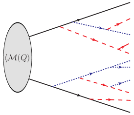
Figure 1: A term contributing to evolution of the conjugate amplitude (it contributes to $\mathbf{A}_{9}$). Red dashed lines represent the emission of soft gluons and collinear partons are represented by blue dotted lines. Loops (Sudakov factors) have been neglected to avoid clutter. We draw all particles heading to the right, away from the hard process, including incoming particles. In contrast, evolution of the amplitude will have all particles drawn heading to the left and away from the hard process.

In this section we present the algorithm. It is Markovian and interleaves soft emissions and virtual corrections with collinear emissions and virtual corrections, see Figure 1. Successive real emissions are strongly ordered in an appropriately defined transverse momentum. We will present two variants of the algorithm, which we refer to as A and B. The two differ only in where we put the soft-collinear emissions: in A they are in the soft sector and in B they are in the collinear sector. The second approach allows us to exploit the colour-diagonal nature of collinear emissions and it makes kinematic recoil more straightforward to implement. Variant A has the virtue that it is an almost trivial extension of the purely soft evolution presented in SoftEvolutionAlgorithm . We present both A and B with the momentum mappings after each real emission parametrised into two initially unspecified functions. This is so the algorithm is able to accommodate partonic recoil. Later, in Section 2.4, we discuss specific examples of recoil in action. For processes with coloured incoming partons, the algorithm should be convoluted with parton distributions functions. We leave a full description of how to do this to Section 4.

Before plunging in, we should explain the theoretical basis for what follows. Our algorithm is based on Feynman diagram calculations SuperleadingLogs ; ColoumbGluonsOrdering ; SoftEvolutionAlgorithm ; Dokshitzer:1991wu ; Dokshitzer:1977sg ; DOKSHITZER1980269 ; Bassetto:1984ik and, in its present form, captures all of the logarithms associated with the leading amplitude-level singularities. Therefore the algorithm captures leading logarithms from wide-angle soft emissions, hard-collinear emissions and simultaneously soft and collinear emissions. This means the algorithm is guaranteed to capture only the most leading logarithms at cross-section level. That said, it is also able to capture the leading single non-global logarithms, even if the global part is double-logarithmic, as is the case with the hemisphere jet mass for example (see Section 4). For any process involving incoming hadrons or measured outgoing hadrons, the single logarithms from DGLAP evolution are recovered as well (i.e. parton distribution function and by a simple extension fragmentation function evolution). We believe our framework to be sufficiently flexible that we can, in the future, extend it beyond the LL approximation.

2.1 Parton branching with interleaved soft and collinear evolution (A)

The algorithm evolves a hard-scattering matrix, $\mathbf{H}(Q;\{p\})$, which is defined at some hard scale $Q$ and is a function of the hard-particle four-momenta, $\{p\}$. It does so by dressing with successive soft and/or collinear real emissions and virtual corrections. $\mathbf{H}(Q;\{p\})$ is a tensor in the product space of colour and helicity, defined as $\mathbf{H}(Q;\{p\})\equiv(\left|\mathrm{colour}\right\rangle\otimes\left|\mathrm{spin}\right\rangle)\otimes(\left\langle\mathrm{colour}\right|\otimes\left\langle\mathrm{spin}\right|)$. The hard-scattering matrix is defined so that $\mathrm{Tr}\,\mathbf{H}(Q;\{p\})$ is the hard matrix element squared, summed over colour and spin. Successive real emissions are added via ‘rectangular’ operators, which act as a map increasing the dimension of the representation of $\mathrm{SU}(3)\times\mathrm{E}(2)$ in which $\mathbf{H}(Q;\{p\})$ resides. The virtual evolution operators are ‘square’ and preserve the representation of $\mathbf{H}(Q;\{p\})$. Specifically,

$$\begin{split}\mathrm{d}\sigma_{0}&=\mathrm{Tr}\left(\mathbf{V}_{\mu,Q}\mathbf{H}(Q;\{p\})\mathbf{V}^{\dagger}_{\mu,Q}\right)=\mathrm{Tr}\,\mathbf{A}_{0}(\mu;\{p\}),\\ \mathrm{d}\sigma_{1}&=\int\prod_{i=1}^{n_{\text{H}}+1}\mathrm{d}^{4}p_{i}\,\mathrm{Tr}\left(\mathbf{V}_{\mu,q_{1\,\bot}}\mathbf{D}_{1}\mathbf{V}_{q_{1\,\bot},Q}\mathbf{H}(Q;\{p\})\mathbf{V}^{\dagger}_{q_{1\,\bot},Q}\mathbf{D}^{\dagger}_{1}\mathbf{V}^{\dagger}_{\mu,q_{1\,\bot}}\right)\mathrm{d}\Pi_{1}\\ &\;=\mathrm{Tr}\,\mathbf{A}_{1}(\mu;\{\tilde{p}\}\cup q_{1})\,\mathrm{d}\Pi_{1},\\ \mathrm{d}\sigma_{n}&\;=\mathrm{Tr}\,\mathbf{A}_{n}(\mu;\{p\}_{n})\prod^{n}_{i=1}\mathrm{d}\Pi_{i},\end{split}$$ (1)

where

$$\mathbf{A}_{n}(q_{\bot};\{\tilde{p}\}_{n-1}\cup q_{n})=\int\prod_{i=1}^{n_{\text{H}}+n}\mathrm{d}^{4}p_{i}\mathbf{V}_{q_{\bot},q_{n\,\bot}}\mathbf{D}_{n}\mathbf{A}_{n-1}(q_{n\,\bot};\{p\}_{n-1})\mathbf{D}^{\dagger}_{n}\mathbf{V}^{\dagger}_{q_{\bot},q_{n\,\bot}}\Theta(q_{\bot}\leq q_{n\,\bot}).$$ (2)

At each step, the emission operators ($\mathbf{D}_{n}$) add one new particle, of four-momentum $q_{n}$, to the set $\{p\}_{n-1}$, to produce the set $\{p\}_{n}$. We use $p_{j}\in\{p\}_{n}=\{P_{1},P_{2},\cdots P_{n_{\text{H}}},q_{1},\cdots q_{n}\}$ to denote the momentum of the $j^{\text{th}}$ parton and $1<j<n_{\text{H}}+n$, where $n_{\text{H}}$ is the number of partons associated with the original hard process and $n$ is the number of emitted partons. Hidden in the emission operators is a map from $\{p\}_{n-1}$ to a new set, $\{\tilde{p}\}_{n-1}$. The difference between these two sets is determined by the way we implement energy-momentum conservation (i.e. the recoil prescription) and it is why there is an extra integral over $p_{i}$ (it is not a phase-space integral). The virtual evolution operators $\mathbf{V}_{a,b}$ encode the loop corrections. To avoid cumbersome notation we write $\{p\}_{n}=\{\tilde{p}\}_{n-1}\cup\{q_{n}\}$ is the set of $n$ momenta including the last emission, $q_{n}$. We have not yet defined the ordering variable, $q_{i\perp}$; we will do that shortly. A generalised observable $\Sigma$, with measurement function $u_{n}(q_{1},...,q_{n})$, is then given by

$$\begin{split}\Sigma(\mu)&=\int\sum_{n}\mathrm{d}\sigma_{n}\,u_{n}(q_{1},...,q_{n}),\\ &=\int\sum_{n}\left(\prod^{n}_{i=1}\mathrm{d}\Pi_{i}\right)\mathrm{Tr}\,\mathbf{A}_{n}(\mu;\{p\}_{n})\,u_{n}(q_{1},...,q_{n}),\end{split}$$ (3)

where $\mathrm{d}\Pi_{i}$ is the phase-space for the $i^{\text{th}}$ emission (see below). $\mu$ should be taken either to $0$ or to the scale below which the observable is inclusive over all radiation. The virtual (Sudakov) evolution operator is

$$\mathbf{V}_{a,b}= \,\mathrm{P}\,\exp\left[-\frac{\alpha_{s}}{\pi}\sum_{i<j}\int^{b}_{a}\frac{\mathrm{d}k^{(ij)}_{\bot}}{k^{(ij)}_{\bot}}(-\mathbb{T}^{g}_{i}\cdot\mathbb{T}^{g}_{j})\left\{\int\frac{\mathrm{d}y\,\mathrm{d}\phi}{4\pi}(k^{(ij)}_{\bot})^{2}\frac{\tilde{p}_{i}\cdot\tilde{p}_{j}}{(\tilde{p}_{i}\cdot k)(\tilde{p}_{j}\cdot k)}\theta_{ij}(k)-i\pi\,\tilde{\delta}_{ij}\right\}\right.$$

$$\;\left.\times\mathcal{R}^{\mathrm{soft}}_{ij}(k,\{\tilde{p}\})-\frac{\alpha_{s}}{\pi}\sum_{i}\int^{b}_{a}\frac{\mathrm{d}k^{(i\vec{n})}_{\bot}}{k^{(i\vec{n})}_{\bot}}\sum_{\upsilon\in\{q,g\}}\mathbb{T}^{\bar{\upsilon}\,2}_{i}\int\frac{\mathrm{d}z\,\mathrm{d}\phi}{8\pi}\,\overline{\mathcal{P}}^{\,\circ}_{\upsilon\upsilon_{i}}(z)\,\theta_{i}(k)\,\mathcal{R}^{\mathrm{coll}}_{i}(k,\{\tilde{p}\})\right],$$ (4)

where $i$ and $j$ run over all external legs (those from the initial hard process and also previous emissions in the evolution). $\tilde{\delta}_{ij}=1$ if both partons $i$, $j$ are incoming or both outgoing and $\tilde{\delta}_{ij}=0$ otherwise. $\theta_{ij}(k)=\Theta(p_{i}\cdot p_{j}-k\cdot(p_{j}+p_{i}))$ and ensures that the phase space of the integration corresponds to that of a real gluon. Likewise, the $z$ integral is over the range

$$z\in\left[\frac{\alpha}{2}-\frac{1}{2}\sqrt{\alpha^{2}-\frac{4k_{\perp}^{(i\vec{n})\,2}}{(n.p)^{2}}}\,,\;\frac{\alpha}{2}+\frac{1}{2}\sqrt{\alpha^{2}-\frac{4k_{\perp}^{(i\vec{n})\,2}}{(n.p)^{2}}}\right],\quad\alpha=\frac{2p\cdot p_{i}+p_{i}\cdot n\,p\cdot n}{(p\cdot n)^{2}}\,,$$ (5)

which can be expressed via a single theta function

$$\theta_{i}(k)=\Theta((n\cdot p_{i}-n\cdot k)n\cdot p+2p\cdot p_{i}-2p\cdot k).$$

The vectors $p$ and $n=(1,\vec{n})$ will be defined shortly: to LL accuracy $p=p_{i}$ and $\alpha=1$. $\upsilon_{i},\upsilon\in\{q,g\}$ label parton species. $\bar{\upsilon}=g$ in all cases except when $\upsilon_{i}=g$ and $\upsilon=q$, then $\bar{\upsilon}=q$. $\overline{\mathcal{P}}_{\upsilon\upsilon_{i}}^{\circ}$ is the $\upsilon_{i}\rightarrow\upsilon$ hard-collinear splitting function and it is defined in Appendix A along with the conventions we use for helicity states and antiparticles. $\mathcal{R}^{\mathrm{soft}}_{ij}(k,\{p\})$ and $\mathcal{R}^{\mathrm{coll}}_{i}(k,\{p\})$ are concerned with the recoil prescription and are included to preserve unitarity, they are defined in (11) and (12) below. $k_{\perp}^{(ij)}$ and $y$ are the transverse momentum and rapidity in the $ij$ zero-momentum frame. To make the (unitarity) link to the real emissions more explicit, we choose not to use the substitution

$$(k^{(ij)}_{\bot})^{2}\frac{\tilde{p}_{i}\cdot\tilde{p}_{j}}{(\tilde{p}_{i}\cdot k)(\tilde{p}_{j}\cdot k)}=2.$$ (6)

The real-emission operator is built using two operators:

$$\begin{split}&\mathbf{S}_{i}=\sum_{j}\left(\frac{q^{(j\vec{m})}_{i\,\bot}}{2\tilde{p}_{j}\cdot q_{i}}\mathbb{T}^{g}_{j}\otimes(\tilde{p}_{j}\cdot\epsilon^{*}_{+}(q_{i})\mathbb{S}^{1_{i}}+\tilde{p}_{j}\cdot\epsilon^{*}_{-}(q_{i})\mathbb{S}^{-1_{i}})\right)\,\mathfrak{R}^{\mathrm{soft}}_{ij}(\{p\},\{\tilde{p}\},q_{i}),\\ &\mathbf{C}_{i}=\sum_{j}\frac{q^{(j\vec{n})}_{i\,\bot}}{2\sqrt{z_{i}}}\Delta_{ij}\,\overline{\mathbf{P}}_{ij}\,\mathfrak{R}^{\mathrm{coll}}_{ij}(\{p\},\{\tilde{p}\},q_{i}),\end{split}$$ (7)

such that $\mathbf{D}_{i}$ acts as

$$\begin{split}...\mathbf{D}_{i}\mathbf{\mathcal{O}}\mathbf{D}^{\dagger}_{i}...=...\mathbf{S}_{i}\mathbf{\mathcal{O}}\mathbf{S}^{\dagger}_{i}...+...\mathbf{C}_{i}\mathbf{\mathcal{O}}\mathbf{C}^{\dagger}_{i}....\end{split}$$ (8)

$j$ again runs over all external legs and $i$ labels the emitted parton. $\mathbf{S}_{i}$ generates soft emissions and $\mathbf{C}_{i}$ hard-collinear emissions. The symbol $\Delta_{ij}$ is defined so that $\Delta_{ij}\Delta_{ik}=\delta_{jk}$ and $\delta^{\mathrm{final}}_{j}$ ($\delta^{\mathrm{initial}}_{j}$) is unity when parton $j$ is in the final (initial) state and zero otherwise. $\overline{\mathbf{P}}_{ij}$ are the amplitude-level hard-collinear splitting functions and are defined in Appendix A. The splitting functions encode DGLAP evolution Dokshitzer:1977sg ; Gribov:1972ri ; APSplitting including the spin-dependence. $\mathbb{T}^{g}_{i}$ is a basis independent colour charge operator. We have indexed each $\mathbb{T}^{g}_{i}$ with the leg on which it acts, $i$, and by whether it corresponds to the emission of a gluon or not (i.e. the index $q$ refers to a $g\to q\bar{q}$ splitting). $\mathbb{S}^{s_{i}}$ updates the helicity state by adding the helicity of the emitted parton, $s_{i}$. The operators $\mathbb{S}$ and $\mathbb{T}$ are also defined in Appendix A.

In the soft sector we have introduced an auxiliary vector $\vec{m}$. It is uniquely determined, but only at cross-section level, since we require $q^{(i\vec{m})}_{\bot}q^{(j\vec{m}^{\prime})}_{\bot}|_{p_{i}\neq p_{j}}=(q^{(ij)}_{\bot})^{2}$, which corresponds to choosing $\vec{m}$ to lie in the direction of $j$ and $\vec{m}^{\prime}$ (the corresponding vector in the conjugate amplitude) in the direction of $i$. It is only ever this combination that appears at cross-section level. In the collinear sector, the momentum fraction $z_{i}$ is defined by (see Figure 2):

$$z_{i} =\frac{\tilde{p}_{j}\cdot n}{p\cdot n}~{}~{}\text{for final-state emissions}$$

$$\text{and}~{}~{}~{}~{}z_{i} =\frac{{p}_{j}\cdot n}{p\cdot n}~{}~{}\text{for initial-state emissions},$$ (9)

where the light-like four-vector $n$ satisfies $n\cdot q^{(j\vec{n})}_{i\perp}=0$. The light-like four-vector $p$ satisfies $p\cdot q^{(j\vec{n})}_{i\perp}=0$. Neglecting terms suppressed by the transverse momentum of the emission (which is permissible in the LL approximation) we may take $p=p_{j}$ for final-state emissions and $p=\tilde{p}_{j}$ for initial-state emissions, in which case $z_{i}$ is the light-cone momentum fraction. The precise definition of $p$ is dependent on the recoil prescription, as we illustrate in Section 2.4.

Now we can define the ordering variable, i.e. the definition of $a$ and $b$ in the Sudakov operator $\mathbf{V}_{a,b}$. We use transverse momentum ordering, where the transverse momentum should be defined by the parent partons of the emitted parton. Doing this means that we really ought not to sum over partons in (7) and we should replace (2) by

$$\mathbf{A}_{n}=\sum_{j_{n},j_{n}^{\prime}}\int\prod_{i=1}^{n_{\text{H}}+n}\mathrm{d}^{4}p_{i}\mathbf{V}_{q_{\bot},q_{n\,\bot}}\mathbf{D}_{n}^{j_{n}}\mathbf{A}_{n-1}\mathbf{D}_{n}^{j_{n}^{\prime}\dagger}\mathbf{V}^{\dagger}_{q_{\bot},q_{n\,\bot}}\Theta(q_{\bot}\leq q_{n\,\bot})$$ (10)

where $\mathbf{D}_{n}^{j_{n}}$ is defined by

$$\mathbf{D}_{n}=\sum_{j_{n}}\mathbf{D}_{n}^{j_{n}}~{}.$$

The ordering variable is then $q_{n\bot}=q_{n}^{(j_{n}j_{n}^{\prime})}$ if the emission is soft or $q_{n\bot}=q_{n}^{(j_{n},\vec{n})}$ if the emission is collinear. At LL, this choice of ordering variable is somewhat arbitrary but being a transverse momentum it is able to generate the super-leading logarithms correctly ColoumbGluonsOrdering . That said, it is not equivalent to the ordering indicated by the results in ColoumbGluonsOrdering ; ColoumbGluonsOrderingLetter , which is based on fixed-order Feynman diagram calculations. We have not yet figured out a way to implement the latter ordering to all orders. In the remainder of the paper, we will use the simpler (though potentially misleading) notation of equation (2).

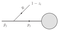
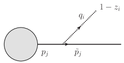
Figure 2: Defining the kinematics: (a) $q_{i}$ is emitted off an incoming leg; (b) $q_{i}$ is emitted off an outgoing leg.

The recoil functions, $\mathfrak{R}^{\mathrm{soft}\,*}_{ij}\,\mathfrak{R}^{\mathrm{soft}}_{ij^{\prime}}$ and $\mathfrak{R}^{\mathrm{coll}\,*}_{ij}\,\mathfrak{R}^{\mathrm{coll}}_{ij}$, encode the maps that implement energy-momentum conservation. As the algorithm proceeds, each $\mathfrak{R}^{\mathrm{soft}}_{ij}$ and $\mathfrak{R}^{\mathrm{coll}}_{ij}$ will always collect into the pairs just given. The functions only ever appear singularly to aid book keeping. The recoil functions should be constructed out of delta functions and algebraic pre-factors relating the momentum from the current step in the algorithm, $\{p\}$, to the momentum that will be carried forwards to the next step of the algorithm, $\{\tilde{p}\}$ and $q_{i}$. $\mathcal{R}^{\mathrm{soft}}_{ij}$ and $\mathcal{R}^{\mathrm{coll}}_{i}$ are fixed by $\mathfrak{R}^{\mathrm{soft}}_{ij}$ and $\mathfrak{R}^{\mathrm{coll}}_{ij}$, i.e.

$$\int\prod_{k}\mathrm{d}^{4}p_{k}\,\mathfrak{R}^{\mathrm{soft}\,*}_{ij}(\{p\},\{\tilde{p}\},q_{i})\mathfrak{R}^{\mathrm{soft}}_{ij^{\prime}}(\{p\},\{\tilde{p}\},q_{i})=\mathcal{R}^{\mathrm{soft}}_{jj^{\prime}}(q_{i},\{\tilde{p}\}),$$ (11)

and

$$\int\prod_{k}\mathrm{d}^{4}p_{k}\,\mathfrak{R}^{\mathrm{coll}\,*}_{ij}(\{p\},\{\tilde{p}\},q_{i})\mathfrak{R}^{\mathrm{coll}}_{ij}(\{p\},\{\tilde{p}\},q_{i})=\mathcal{R}^{\mathrm{coll}}_{j}(q_{i},\{\tilde{p}\}).$$ (12)

In the LL approximation, $\mathcal{R}^{\mathrm{soft}}_{jj^{\prime}}=\mathcal{R}^{\mathrm{coll}}_{j}=1$. $\mathbf{S}_{i}$ generates soft emissions and one might suppose that a suitable choice of recoil (to LL accuracy) is

$$\mathfrak{R}^{\mathrm{soft}}_{ij}\mathfrak{R}^{\mathrm{soft}\,*}_{ij^{\prime}}=\prod_{k}\delta^{4}(p_{k}-\tilde{p}_{k}).$$ (13)

We will shortly see that things are not quite so simple, and that this requires modification. $\mathbf{C}_{i}$ generates hard-collinear emissions, however only the longitudinal component of the recoil is hard. Therefore, in the LL approximation, we may implement recoils in the collinear sector via

$$\mathfrak{R}^{\mathrm{coll}\,*}_{ij}\mathfrak{R}^{\mathrm{coll}}_{ij}=\left(\delta^{4}(p_{j}-z^{-1}_{i}\tilde{p}_{j})\delta^{\mathrm{final}}_{j}+\delta^{4}(p_{j}-z_{i}\tilde{p}_{j})\delta^{\mathrm{initial}}_{j}\right)\prod_{k\neq j}\delta^{4}(p_{k}-\tilde{p}_{k}).$$ (14)

Finally, the phase-space is included via

$$\begin{split}\mathrm{d}\Pi_{i}&=\frac{2\alpha_{s}}{\pi^{2}q^{2}_{i\,\bot}}\frac{\mathrm{d}^{3}q_{i}}{2E_{i}}.\end{split}$$ (15)

The pre-factor has been included to simplify the definitions of $\mathbf{S}_{i}$ and $\mathbf{C}_{i}$, as well as to make each term in the algorithm dimensionless and keep explicit dependence on the ordering variable in $\mathbf{D}_{i}$. To simplify the notation, in (15) and elsewhere, we will drop the dipole labels on transverse momenta. It should be clear from the context which partons are intended. In the case of (15), it means we should use the transverse momentum defined by the parent parton and the vector $\vec{n}$ in the case of collinear emissions or $q_{\perp}^{(ij)}$ in the case of soft emissions. It is often useful to note that

$$\begin{split}\mathrm{d}\Pi_{i}&=\frac{2\alpha_{s}}{\pi}\frac{\mathrm{d}q_{i\,\bot}}{q_{i\,\bot}}\frac{\mathrm{d}z_{i}}{1-z_{i}}\frac{\mathrm{d}\phi_{i}}{2\pi}=\frac{2\alpha_{s}}{\pi}\frac{\mathrm{d}q_{i\,\bot}}{q_{i\,\bot}}\frac{\mathrm{d}y\,\mathrm{d}\phi}{2\pi},\end{split}$$ (16)

where $y$ is the rapidity in the frame defining $q_{i\,\bot}$. Using these last two relations the link between real emissions and virtual corrections is clear, i.e. the square of the emission operators $\int\mathbf{D}_{i}^{\dagger}\mathbf{D}_{i}\,\mathrm{d}\Pi_{i}$ is, for $e^{+}e^{-}$ collisions, equal to minus twice the real part of the exponent in (2.1).

Using the naive recoil prescription of (13) and (14), the array of parton momenta gets modified after a collinear emission, generated by $\overline{\mathbf{P}}_{ij}$, but not after a soft emission (except to add one new soft gluon of course). Specifically, this means acting with $\overline{\mathbf{P}}_{ij}\mathfrak{R}^{\mathrm{coll}}_{ij}$ maps $p_{j}\mapsto\tilde{p}_{j}=z_{i}p_{j}+\mathcal{O}(q_{\bot})$ (for final state partons), and a parton with momentum $q_{i}=(1-z)p_{j}+\mathcal{O}(q_{\bot})$ is added. As usual, $p_{j}$ is the momentum of parton $j$ prior to the action of $\overline{\mathbf{P}}_{ij}\mathfrak{R}^{\mathrm{coll}}_{ij}$. A more careful treatment of momenta is not required to reproduce the leading logarithms for many observables. However, any observable dependent upon parton distribution functions or fragmentation functions will be incorrectly calculated because this naive recoil prescription does not reproduce DGLAP evolution. This is because the terms with soft-collinear poles are handled in the ‘soft side’ of the algorithm and do not conserve longitudinal momentum. This manifests as DGLAP evolution with an incorrect plus prescription, i.e.

$$\left(\frac{1+z^{2}}{1-z}\right)_{+}=\left(\frac{2}{1-z}\right)_{+}-(1+z)_{+}\stackrel{{\scriptstyle\mathrm{variant}\,\mathrm{A}}}{{\longmapsto}}-(1+z)_{+},$$ (17)

as the soft poles have been removed from the hard-collinear splitting functions defining $\overline{\mathbf{P}}_{ij}$. On the flip side, the algorithm works well for event shape observables in $e^{+}e^{-}$ collisions. We will refer to the framework in this section as variant A of the algorithm. Within variant A, this problem could be solved by implementing a universal recoil for all emissions, soft and collinear, i.e.

$$\int\prod_{k}\mathrm{d}^{4}\,p_{k}\,\mathfrak{R}^{\mathrm{coll}}_{ij}\mathfrak{R}^{\mathrm{coll}\,*}_{ij} =\int\prod_{k}\mathrm{d}^{4}p_{k}\,\sum_{j^{\prime}}\,\mathfrak{R}^{\mathrm{soft}}_{ij}\mathfrak{R}^{\mathrm{soft}\,*}_{ij^{\prime}}.$$ (18)

We will not consider universal recoils in this paper and will instead solve this ‘plus prescription problem’ another way; by putting the soft-collinear emissions in the collinear sector of the algorithm. Doing this will lead us to variant B of the algorithm. In Section 2.4, we will use the insight gained from formulating B to show how to solve the plus-prescription problem within the framework of A.

2.2 Parton branching using complete collinear splitting functions (B)

Soft-collinear poles can be exchanged reasonably simply between eikonal currents and collinear splitting functions. We will now define variant B of our algorithm, which restores the soft-collinear poles in the collinear splitting functions and removes them from the eikonal currents. This is a good thing to do for two reasons:

1. Collinear evolution is generated by unit operators in colour space. Making this manifest for the soft-collinear poles simplifies the colour evolution of the algorithm.

2. Putting the soft-collinear poles into the collinear ‘side’ of the algorithm simplifies the recoil prescription because every collinear emission has a uniquely identifiable parent.

Variant B is very similar in form to variant A:

$$\begin{split}\mathbf{S}_{i}&=\sum_{j}\left(\frac{q^{(j\vec{m})}_{i\,\bot}}{2\tilde{p}_{j}\cdot q_{i}}\mathbb{T}^{g}_{j}\otimes(\tilde{p}_{j}\cdot\epsilon^{*}_{+}(q_{i})\mathbb{S}^{1_{i}}+\tilde{p}_{j}\cdot\epsilon^{*}_{-}(q_{i})\mathbb{S}^{-1_{i}})\right)\,\mathfrak{R}^{\mathrm{soft}}_{ij}(\{p\},\{\tilde{p}\},q_{i}),\\ \mathbf{C}_{i}&=\sum_{j}\frac{q^{(j\vec{n})}_{i\,\bot}}{2\sqrt{z_{i}}}\Delta_{ij}\,\mathbf{P}_{ij}\,\mathfrak{R}^{\mathrm{coll}}_{ij}(\{p\},\{\tilde{p}\},q_{i}),\end{split}$$ (19)

with

$$\begin{split}...\mathbf{D}_{i}\mathbf{\mathcal{O}}\mathbf{D}^{\dagger}_{i}...&=...\mathbf{S}_{i}\mathbf{\mathcal{O}}\mathbf{S}^{\dagger}_{i}\,\mathfrak{f}_{jj^{\prime}}(q_{i},\{p\},\{\tilde{p}\})...+...\mathbf{C}_{i}\mathbf{\mathcal{O}}\mathbf{C}^{\dagger}_{i}...\,.\end{split}$$ (20)

The form of $\mathbf{S}_{i}$ is the same as in A and the Sudakov changes as

$$\mathbf{V}_{a,b}= \,\mathrm{P}\,\exp\left[-\frac{\alpha_{s}}{\pi}\sum_{i<j}\int^{b}_{a}\frac{\mathrm{d}k^{(ij)}_{\bot}}{k^{(ij)}_{\bot}}(-\mathbb{T}^{g}_{i}\cdot\mathbb{T}^{g}_{j})\left\{\int\frac{\mathrm{d}y\,\mathrm{d}\phi}{4\pi}(k^{(ij)}_{\bot})^{2}\frac{\tilde{p}_{i}\cdot\tilde{p}_{j}}{(\tilde{p}_{i}\cdot k)(\tilde{p}_{j}\cdot k)}\theta_{ij}(k)\,\right.\right.$$ (21)

$$\;\;\left.\left.\times\mathcal{F}_{ij}(k,\{\tilde{p}\})-i\pi\tilde{\delta}_{ij}\right\}\mathcal{R}^{\mathrm{soft}}_{ij}-\frac{\alpha_{s}}{\pi}\sum_{i}\int^{b}_{a}\frac{\mathrm{d}k^{(i\vec{n})}_{\bot}}{k^{(i\vec{n})}_{\bot}}\sum_{\upsilon}\mathbb{T}^{\bar{\upsilon}\,2}_{i}\int\frac{\mathrm{d}z\,\mathrm{d}\phi}{8\pi}\mathcal{P}^{\,\circ}_{\upsilon\upsilon_{i}}\,\theta_{i}(k)\,\mathcal{R}^{\mathrm{coll}}_{i}\right].$$

The only changes relative to variant A are the appearance of $\mathfrak{f}_{jj^{\prime}}(q_{i},\{p\},\{\tilde{p}\})$ and $\mathcal{F}_{ij}(k,\{\tilde{p}\})$, which specify the prescription for the subtraction of soft-collinear poles from the eikonal currents, and the replacement of $\overline{\mathbf{P}}_{ij}$ with $\mathbf{P}_{ij}$. Explicit dependence on $\mathbf{P}_{ij}$ in $\mathbf{C}_{i}$ means that $\mathbf{C}_{i}\mathcal{O}\mathbf{C}^{\dagger}_{i}$ now contains the full spin-dependent DGLAP splitting functions HelicitySplitting . Unitarity requires that

$$\int\prod_{i}\mathrm{d}^{4}\,p_{i}\,\mathfrak{f}_{jj^{\prime}}(q_{i},\{p\},\{\tilde{p}\})\,\mathfrak{R}^{\mathrm{soft}\,*}_{ij}\mathfrak{R}^{\mathrm{soft}}_{ij^{\prime}}=\mathcal{F}_{jj^{\prime}}(q_{i},\{\tilde{p}\})\,\mathcal{R}^{\mathrm{soft}}_{ij}(q_{i},\{\tilde{p}\}).$$ (22)

The functional forms of $\mathfrak{f}_{jj^{\prime}}(q_{i},\{p\},\{\tilde{p}\})$ and $\mathcal{F}_{jj^{\prime}}(q_{i},\{\tilde{p}\})$ are uniquely fixed by the choice of $\mathfrak{R}^{\mathrm{coll}}_{ij}$ and $\mathfrak{R}^{\mathrm{soft}}_{ij}$ once we have fixed $\mathbf{P}_{ij}$. Specifically, we can derive variant B from A by adding and subtracting a function:

$$\mathbf{S}^{\mathrm{B}}_{i}\mathcal{O}\mathbf{S}^{\mathrm{B}\,\dagger}_{i}\,\mathrm{d}\Pi_{i}+\mathbf{C}^{\mathrm{B}}_{i}\mathcal{O}\mathbf{C}^{\mathrm{B}\,\dagger}_{i}\,\mathrm{d}\Pi_{i}=\underbrace{\mathbf{S}^{\mathrm{A}}_{i}\mathcal{O}\mathbf{S}^{\mathrm{A}\,\dagger}_{i}\,\mathrm{d}\Pi_{i}-\mathbf{s}_{i}\mathcal{O}\mathbf{s}^{\dagger}_{i}}_{\equiv\mathbf{S}^{\mathrm{B}}_{i}\mathcal{O}\mathbf{S}^{\mathrm{B}\,\dagger}_{i}\,\mathrm{d}\Pi_{i}}+\underbrace{\mathbf{C}^{\mathrm{A}\,\dagger}_{i}\mathcal{O}\mathbf{C}^{\mathrm{A}}_{i}\,\mathrm{d}\Pi_{i}+\mathbf{s}_{i}\mathcal{O}\mathbf{s}^{\dagger}_{i}}_{\equiv\mathbf{C}^{\mathrm{B}}_{i}\mathcal{O}\mathbf{C}^{\mathrm{B}\,\dagger}_{i}\,\mathrm{d}\Pi_{i}},$$ (23)

where we have labelled each operator with a superscript indicating which variant it corresponds to and where $\mathcal{O}$ is some general operator in colour and spin. The subtraction term was constructed so that

$$\mathbf{s}_{i}\mathcal{O}\mathbf{s}^{\dagger}_{i}\equiv\sum_{j}\frac{(q^{(j\vec{n})}_{i\,\bot})^{2}}{4z_{i}}(\mathbf{P}_{ij}\mathcal{O}\mathbf{P}^{\dagger}_{ij}-\overline{\mathbf{P}}_{ij}\mathcal{O}\overline{\mathbf{P}}^{\dagger}_{ij})\,\mathfrak{R}^{\mathrm{coll}}_{ij}\mathfrak{R}^{\mathrm{coll}\,*}_{ij}\,\mathrm{d}\Pi_{i}$$ (24)

and after some manipulation is equal to

$$\mathbf{s}_{i}\mathcal{O}\mathbf{s}^{\dagger}_{i}=\frac{2\alpha_{s}}{\pi}\sum_{j} \mathbb{T}^{g}_{j}\otimes\left(\frac{\mathbb{S}^{1_{i}}}{\left\langle q_{i}\tilde{p}_{j}\right\rangle}+\frac{\mathbb{S}^{-1_{i}}}{[q_{i}\tilde{p}_{j}]}\right)\mathcal{O}\,\mathbb{T}^{g\,\dagger}_{j}\otimes\left(\frac{\mathbb{S}^{1_{i}}}{\left\langle q_{i}\tilde{p}_{j}\right\rangle}+\frac{\mathbb{S}^{-1_{i}}}{[q_{i}\tilde{p}_{j}]}\right)^{\dagger}$$

$$\times q_{i}\cdot\tilde{p}_{j}\frac{\mathrm{d}q^{(j\vec{n})}_{i\,\bot}}{q^{(j\vec{n})}_{i\,\bot}}\frac{\mathrm{d}y\,\mathrm{d}\phi}{2\pi}\theta_{j}(q_{i})\,(\delta^{\mathrm{final}}_{j}+\delta^{\mathrm{initial}}_{j}(\tilde{p}_{j}\leftrightarrow p_{j}))\,\mathfrak{R}^{\mathrm{coll}}_{ij}\mathfrak{R}^{\mathrm{coll}\,*}_{ij}.$$ (25)

$\left\langle q_{i}\tilde{p}_{j}\right\rangle$ and $[q_{i}\tilde{p}_{j}]$ are Weyl products in the spinor-helicity formalism HelicityTechniques . Also note, $\mathbf{s}_{i}\mathcal{O}\mathbf{s}^{\dagger}_{i}$ is equal to the collinear limit of $\mathbf{S}^{\mathrm{A}}_{i}\mathcal{O}\mathbf{S}^{\mathrm{A}\,\dagger}_{i}\,\mathrm{d}\Pi_{i}$ with $q^{(j\vec{m})}_{i\,\bot}\approx q^{(j\vec{n})}_{i\,\bot}$. To see the equality we express polarisation vectors using spinor products,

$$\epsilon^{\mu}(q_{i},\pm 1)=\frac{1}{\sqrt{2}}\frac{\left\langle q_{i}\mp\right|\sigma^{\mu}_{\mp}\left|n\mp\right\rangle}{\left\langle q_{i}\pm|n\mp\right\rangle},$$ (26)

where $\sigma^{\mu}_{\mp}=(\mathbbm{1},\mp\sigma_{1},\mp\sigma_{2},\mp\sigma_{3})^{\mathrm{T}}$ are vectors of Pauli matrices and $n$ is an auxillary light-like vector (best chosen to be either $p_{j}$ or $p_{j^{\prime}}$).

To complete the definition of variant B we must compute $\mathfrak{f}_{jj^{\prime}}(q_{i},\{p\},\{\tilde{p}\})$ and $\mathcal{F}_{jj^{\prime}}(q_{i},\{\tilde{p}\})$. Note that $\mathbf{s}^{\dagger}_{i}\mathbf{s}_{i}$ is proportional to the unit operator in colour and helicity. After taking the trace over helicity space, (23) leads to

$$\sum_{j,j^{\prime}}\mathbb{T}^{g}_{j}\mathcal{O}\mathbb{T}^{g\,\dagger}_{j^{\prime}}\,\frac{\mathrm{d}q^{(jj^{\prime})}_{i\,\bot}}{q^{(jj^{\prime})}_{i\,\bot}}\frac{\mathrm{d}y\,\mathrm{d}\phi}{4\pi}\theta_{jj^{\prime}}(q_{i})\,\mathfrak{R}^{\mathrm{soft}}_{ij}\mathfrak{R}^{\mathrm{soft}\,*}_{ij^{\prime}}\mathfrak{f}_{jj^{\prime}}(q_{i},\{p\},\{\tilde{p}\})=$$

$$\sum_{j,j^{\prime}}\mathbb{T}^{g}_{j}\mathcal{O}\mathbb{T}^{g\,\dagger}_{j^{\prime}}\,\frac{\mathrm{d}q^{(jj^{\prime})}_{i\,\bot}}{q^{(jj^{\prime})}_{i\,\bot}}\frac{\mathrm{d}y\,\mathrm{d}\phi}{4\pi}\theta_{jj^{\prime}}(q_{i})\,\mathfrak{R}^{\mathrm{soft}}_{ij}\mathfrak{R}^{\mathrm{soft}\,*}_{ij^{\prime}}+\sum_{j}\mathbb{T}^{g}_{j}\mathcal{O}\mathbb{T}^{g\,\dagger}_{j}\,\frac{\mathrm{d}q^{(j\vec{n})}_{i\,\bot}}{q^{(j\vec{n})}_{i\,\bot}}\frac{\mathrm{d}y\,\mathrm{d}\phi}{4\pi}\theta_{j}(q_{i})\,\mathfrak{R}^{\mathrm{coll}}_{ij}\mathfrak{R}^{\mathrm{coll}\,*}_{ij}.$$ (27)

We can use colour conservation to factorise the colour operators and simplify the second term on the right-hand side, i.e.

$$\mathfrak{f}_{jj^{\prime}}(q_{i},\{p\},\{\tilde{p}\})=1-\dfrac{\mathrm{d}q^{(j\vec{n})}_{i\,\bot}}{\mathrm{d}q^{(jj^{\prime})}_{i\,\bot}}\,\frac{q^{(jj^{\prime})}_{i\,\bot}\theta_{j}(q_{i})}{q^{(j\vec{n})}_{i\,\bot}\theta_{jj^{\prime}}(q_{i})}\,\frac{\mathfrak{R}^{\mathrm{coll}\,*}_{ij}\mathfrak{R}^{\mathrm{coll}}_{ij}}{\mathfrak{R}^{\mathrm{soft}\,*}_{ij}\mathfrak{R}^{\mathrm{soft}}_{ij^{\prime}}}$$ (28)

and

$$\mathcal{F}_{jj^{\prime}}(q_{i},\{p_{j}\})=1-\dfrac{\mathrm{d}q^{(j\vec{n})}_{i\,\bot}}{\mathrm{d}q^{(jj^{\prime})}_{i\,\bot}}\,\frac{q^{(jj^{\prime})}_{i\,\bot}\theta_{j}(q_{i})}{q^{(j\vec{n})}_{i\,\bot}\theta_{jj^{\prime}}(q_{i})}\,\frac{\mathcal{R}^{\mathrm{coll}}_{j}}{\mathcal{R}^{\mathrm{soft}}_{jj^{\prime}}}.$$ (29)

For a universal recoil it is possible to employ colour conservation and write

$$\sum_{j}\mathbb{T}^{g}_{j}\mathcal{O}\mathbb{T}^{g\,\dagger}_{j}\,\frac{\mathrm{d}q^{(j\vec{n})}_{i\,\bot}}{q^{(j\vec{n})}_{i\,\bot}}\frac{\mathrm{d}y\,\mathrm{d}\phi}{4\pi}\theta_{j}(q_{i})\,\mathfrak{R}^{\mathrm{coll}}_{ij}\mathfrak{R}^{\mathrm{coll}\,*}_{ij}=\sum_{j,j^{\prime}}\mathbb{T}^{g}_{j}\mathcal{O}\mathbb{T}^{g\,\dagger}_{j^{\prime}}\,\frac{\mathrm{d}q^{(j\vec{n})}_{i\,\bot}}{q^{(j\vec{n})}_{i\,\bot}}\frac{\mathrm{d}y\,\mathrm{d}\phi}{4\pi}\theta_{j}(q_{i})\,\mathfrak{R}^{\mathrm{soft}}_{ij}\mathfrak{R}^{\mathrm{soft}\,*}_{ij^{\prime}},$$ (30)

which enables us to re-write (28) as

$$\mathfrak{f}_{jj^{\prime}}(q_{i},\{p\},\{\tilde{p}\})=1-\dfrac{\mathrm{d}q^{(j\vec{n})}_{i\,\bot}}{\mathrm{d}q^{(jj^{\prime})}_{i\,\bot}}\,\frac{q^{(jj^{\prime})}_{i\,\bot}\theta_{j}(q_{i})}{q^{(j\vec{n})}_{i\,\bot}\theta_{jj^{\prime}}(q_{i})}.$$ (31)

In the case of a universal recoil prescription, the effects of the recoil can be factorised out of the emission operators and into a redefinition of the phase space measure. Recoil schemes that may be universal include the more ‘true to Feynman diagrams’ global prescriptions which put momenta of partons higher in the chain of emissions off-shell (e.g. see Bewick:2019rbu and references therein) and schemes which democratically share recoil across a jet or every parton in the shower. Depending on their implementation, such schemes can be universal since they globally redistribute momentum across the whole event as a $n\rightarrow n+1$ parton processes. We leave the specification a universal recoil scheme to future work. For now we re-iterate that it is only when considering effects beyond LL that (31) and (28) differ.

Our implementation of recoil is not unique, and it remains to be seen (by performing analytic calculations at NLL and beyond) the extent to which we will eventually be able to capture the salient sub-leading logarithms in the framework of our algorithm. A slightly different approach would be to start with variant B (recall we started from variant A above) and assume (31) holds true. Variant A could then be constructed but it would now include subtraction functions akin to $\mathfrak{f}_{jj^{\prime}}$. In the case of universal recoils, none of this matters of course.

2.3 Collinear subtractions and the ordering variable

Before moving on, we’d like to present a slightly more general approach to subtracting the soft-collinear contribution. This calculation will shed some light on the role played by the ordering variable. We start by writing

$$\ln{\mathbf{V}}_{ab}=\frac{\alpha_{s}}{2\pi}\sum_{i<j}{\mathbb{T}}_{i}^{g}\cdot{\mathbb{T}}_{j}^{g}\int_{a^{2}}^{b^{2}}\frac{{\rm d}q^{2}}{q^{2}}\int\frac{{\rm d}^{3}k}{2E}\frac{K^{2}(p_{i},p_{j};k)}{\pi}\frac{\ p_{i}\cdot p_{j}}{p_{i}\cdot k\,p_{j}\cdot k}\delta\left(q^{2}-K^{2}(p_{i},p_{j};k)\right)\,\theta_{ij}(k)~{},$$ (32)

which holds for a general definition of the ordering variable, $K^{2}(p_{i},p_{j},k)$. In order to isolate the collinear divergence, we should first expose, and factor, the soft divergence. To do this, it is sufficient to consider any scaling which is linear in the emitted gluon’s momentum components, such that we can re-write

$$\ln{\mathbf{V}}_{ab}=\frac{\alpha_{s}}{2\pi}\sum_{i<j}{\mathbb{T}}_{i}^{g}\cdot{\mathbb{T}}_{j}^{g}\int_{a^{2}}^{b^{2}}\frac{{\rm d}q^{2}}{q^{2}}\int\frac{{\rm d}^{3}k\ }{2E}\frac{K^{2}(p_{i},p_{j};k)}{\pi\,(S\cdot k)^{2}}\frac{\ n_{i}\cdot n_{j}}{n_{i}\cdot n\ n_{j}\cdot n}\delta\left(q^{2}-K^{2}(p_{i},p_{j};k)\right)\theta_{ij}(k),$$ (33)

where $n_{i}=q_{i}/(S\cdot q_{i})$, $n=k/(S\cdot k)$ and $S$ is any time-like four-vector, which we choose to satisfy $S^{2}=1$. The soft divergence is now isolated from the eikonal term, which is singular only in the collinear limits $n_{i,j}\cdot n\to 0$. The collinear divergences can be subtracted. We want the ordering variable to become independent of the other parton’s direction in the collinear limit, such that the entire collinear divergence can be moved into a jet factor that is trivial in colour space.

We choose to re-write the virtual evolution as $\ln{\mathbf{V}}_{ab}=\ln{\mathbf{W}}_{ab}+\ln{\mathbf{K}}_{ab}$, where

$$\ln {\mathbf{W}}_{ab}=\frac{\alpha_{s}}{2\pi}\sum_{i<j}{\mathbb{T}}_{i}^{g}\cdot{\mathbb{T}}_{j}^{g}\int_{a^{2}}^{b^{2}}\frac{{\rm d}q^{2}}{q^{2}}\int\frac{{\rm d}^{3}k\ }{2E}\frac{1}{\pi\,(S\cdot k)^{2}}$$

$$\Bigg{(}K^{2}(p_{i},p_{j};k)\frac{n_{i}\cdot n_{j}}{n_{i}\cdot n\ n\cdot n_{j}}\delta(q^{2}-K^{2}(p_{i},p_{j};k))\,\theta_{ij}(k)$$

$$-\frac{K^{2}(p_{i};k)}{n_{i}\cdot n}\delta(q^{2}-K^{2}(p_{i};k))\theta_{i}(k)-\frac{K^{2}(p_{j};k)}{n_{j}\cdot n}\delta(q^{2}-K^{2}(p_{j};k))\theta_{j}(k)\Bigg{)}\ ,$$ (34)

and colour conservation can now be used to obtain

$$\ln{\mathbf{K}}_{ab}=\frac{\alpha_{s}}{2\pi}\sum_{i}({\mathbb{T}}_{i}^{g})^{2}\int_{a^{2}}^{b^{2}}\frac{{\rm d}q^{2}}{q^{2}}\int\frac{{\rm d}^{3}k\ }{2E}\frac{2}{\pi\,(S\cdot k)^{2}}\frac{K^{2}(p_{i};k)}{n_{i}\cdot n}\delta\left(q^{2}-K^{2}(p_{i};k)\right)\theta_{i}(k)\ .$$ (35)

This factor contains the ordering variable in terms of a single emitter direction, which is the limiting case of the dipole-type definition in each collinear limit, i.e. $K^{2}(p_{i},p_{j},k)\to K^{2}(p_{i};k)$ as $n_{i}\cdot n\to 0$. Given the Lorentz invariance of the virtual evolution and the integration measure we can choose $S=(1,\vec{0})$.

In the case of energy ordering, we obtain the following for the subtracted soft evolution:

$$\ln{\mathbf{W}}_{ab}\Big{|}_{\text{energy}} =\frac{\alpha_{s}}{\pi}\sum_{i<j}{\mathbb{T}}_{i}^{g}\cdot{\mathbb{T}}_{j}^{g}\int_{a}^{b}\frac{{\rm d}E}{E}\int\frac{{\rm d}\Omega}{4\pi}\left(\frac{n_{i}\cdot n_{j}-n_{i}\cdot n-n_{j}\cdot n}{n_{i}\cdot n\ n\cdot n_{j}}\right)$$

$$=\frac{\alpha_{s}}{\pi}\sum_{i<j}{\mathbb{T}}_{i}^{g}\cdot{\mathbb{T}}_{j}^{g}\int_{a}^{b}\frac{{\rm d}E}{E}\;\ln\frac{n_{i}\cdot n_{j}}{2}~{}$$ (36)

where the angular integral can be performed using the same integral that gives rise to angular ordering. And for the collinearly divergent factor:

$$\ln{\mathbf{K}}_{ab}\Big{|}_{\text{energy}}=\frac{\alpha_{s}}{\pi}\sum_{i}({\mathbb{T}}_{i}^{g})^{2}\int_{a}^{b}\frac{{\rm d}E}{E}\int\frac{{\rm d}\Omega}{4\pi}\frac{2}{n_{i}\cdot n}\ .$$ (37)

There is no need for $\theta_{ij}$ since this simply enforces that the emitted gluon should have energy smaller than $\sqrt{\tfrac{1}{2}p_{i}\cdot p_{j}}$ in the $ij$ zero momentum frame, which is automatically satisfied since $a<E<b$.

Now let us consider the case of transverse momentum ordering. This can be implemented through

$$K^{2}(p_{i},p_{j};k)=(k_{\perp}^{(ij)})^{2}=\frac{2\ p_{i}\cdot k\ k\cdot p_{j}}{p_{i}\cdot p_{j}}\ ,$$ (38)

and

$$K^{2}(p;k)\sim 2p\cdot k$$ (39)

where the similarity sign refers to any function which approaches unity in the limit $p\cdot k\to 0$. Making the minimal choice, the full evolution becomes

$$\ln{\mathbf{V}}_{ab}\Big{|}_{k_{T}}=\frac{\alpha_{s}}{\pi}\sum_{i<j}{\mathbb{T}}_{i}^{g}\cdot{\mathbb{T}}_{j}^{g}\int_{a}^{b}\frac{{\rm d}k_{\perp}}{k_{\perp}}\int\frac{{\rm d}z}{1-z}\,\frac{{\rm d}\phi}{2\pi}\;\theta_{ij}(k)$$ (40)

and

$$\ln{\mathbf{K}}_{ab}\Big{|}_{k_{T}} =\frac{\alpha_{s}}{2\pi}\sum_{i}({\mathbb{T}}_{j}^{g})^{2}\int_{a}^{b}\frac{{\rm d}k_{\perp}}{k_{\perp}}\int_{\alpha}^{1}\frac{\text{d}z}{1-z+\alpha}\,\int\frac{\text{d}\phi}{2\pi}$$

$$=\frac{\alpha_{s}}{2\pi}\sum_{i}({\mathbb{T}}_{j}^{g})^{2}\int_{a}^{b}\frac{\text{d}k_{\perp}}{k_{\perp}}\,\int_{0}^{1-\alpha}\frac{\text{d}z}{1-z}\,\int\frac{\text{d}\phi}{2\pi}$$ (41)

where $\alpha=k_{\perp}^{2}/(2S\cdot p_{i})^{2}$. This is the same as the subtraction prescription we introduced in the last section, with the only difference being that the lower limit on the $z$ integral is (approximately) equal to $\alpha$ in that case. Finally, using colour conservation we can compute $\ln{\mathbf{V}}_{ab}-\ln{\mathbf{K}}_{ab}$ and get

$$\ln{\mathbf{W}}_{ab}\Big{|}_{k_{T}} =\frac{\alpha_{s}}{\pi}\sum_{i<j}{\mathbb{T}}_{i}^{g}\cdot{\mathbb{T}}_{j}^{g}\int_{a}^{b}\frac{{\rm d}k_{\perp}}{k_{\perp}}\int\frac{\mathrm{d}y\,{\rm d}\phi}{2\pi}\;(\theta_{ij}(k)-\theta_{i}(k))\,,$$

$$=\frac{\alpha_{s}}{\pi}\sum_{i<j}{\mathbb{T}}_{i}^{g}\cdot{\mathbb{T}}_{j}^{g}\int_{a}^{b}\frac{{\rm d}k_{\perp}}{k_{\perp}}\int\frac{\mathrm{d}y\,{\rm d}\phi}{2\pi}\;\mathcal{F}_{ij}(k)\,\theta_{ij}(k)\,,$$

$$\approx\frac{\alpha_{s}}{\pi}\sum_{i<j}{\mathbb{T}}_{i}^{g}\cdot{\mathbb{T}}_{j}^{g}\int_{a}^{b}\frac{{\rm d}k_{\perp}}{k_{\perp}}\ln\frac{n_{i}\cdot n_{j}}{2}~{},$$ (42)

where the second line illustrates the equivalence with the subtraction scheme presented in the previous section (recall we are ignoring recoil in this section). The approximately-equal-to sign is because we neglect terms suppressed by powers of $k_{\perp}^{2}$. As expected, this finite term is the same as the energy ordering case in equation (36). The form factor $\exp(\ln\mathbf{W})$ captures all of the truly wide-angle soft-gluon physics and is essentially the same as the fifth form factor introduced by Dokshitzer & Marchesini Dokshitzer:2005ek .

2.4 A local recoil prescription

Next we will show how a more sophisticated recoil prescription (than (13) and (14)) can be implemented. The recoil we choose is based on the one in Schumann:2007mg ; Platzer:recoil , but extended to work with colour off-diagonal evolution. The dipole recoil is itself based on Catani-Seymour dipole factorisation and furthers the work in Catani:1996vz so that recoil can be implemented in a dipole parton shower. As a result, this recoil scheme shares similarities with the spectator recoil prescriptions used in modern dipole showers such as Pythia and Dire Pythia8 ; DIRE . The idea is not to present a definitive recoil prescription but rather to illustrate how one can be implemented in our algorithm. To that end, we calculate $\mathcal{F}_{ij}$ and $\mathfrak{R}^{\mathrm{coll}}_{ij}$. We also provide a short discussion on the successes and limitations of the prescription. We then go on to show that, at LL, the recoil prescription can be reduced to the naive recoil prescription when implemented in variant B (but not variant A).

To keep things as simple as possible, we will consider the dipole recoil scheme in the case of only coloured final-state partons. The extension to coloured initial-state partons is straightforward and can be found by following Section 3.2 of Platzer:recoil . First we will summarise the dipole recoil for colour-diagonal evolution. It works by adding a spectator particle to the standard description of a $1\rightarrow 2$ collinear splitting ($p_{j}\rightarrow\tilde{p}_{j},q_{i}$). This spectator particle absorbs the recoil from the splitting, which would otherwise put $p_{j}$ off-shell. The spectator particle has a second function: to specify the frame in which the transverse momentum of the emission is computed. In Platzer:recoil it was shown that one can obtain the correct colour-diagonal evolution by choosing the parton that is colour connected to parton $j$ as the spectator. We will denote the momentum of the spectator parton by $p_{j^{\mathrm{LR}}}$ (the reason for the LR subscript will become clear). The Sudakov decomposition is

$$\begin{split}\tilde{p}_{j}&=z_{i}p_{j}-k_{\bot}+\frac{(q^{(jj^{\mathrm{LR}})}_{\bot})^{2}}{z_{i}}\frac{p_{j^{\mathrm{LR}}}}{2p_{j}\cdot p_{j^{\mathrm{LR}}}},\qquad(q^{(jj^{\mathrm{LR}})}_{\bot})^{2}=-k_{\bot}^{2},\\ q_{i}&=(1-z_{i})p_{j}+k_{\bot}+\frac{(q^{(jj^{\mathrm{LR}})}_{\bot})^{2}}{1-z_{i}}\frac{p_{j^{\mathrm{LR}}}}{2p_{j}\cdot p_{j^{\mathrm{LR}}}},\\ \tilde{p}_{j^{\mathrm{LR}}}&=\left(1-\frac{(q^{(jj^{\mathrm{LR}})}_{\bot})^{2}}{z_{i}(1-z_{i})}\frac{1}{2p_{j}\cdot p_{j^{\mathrm{LR}}}}\right)p_{j^{\mathrm{LR}}},\qquad k_{\bot}\cdot p_{j}=k_{\bot}\cdot p_{j^{\mathrm{LR}}}=0.\end{split}$$ (43)

This now defines a $2\rightarrow 3$ splitting ($p_{j},p_{j^{\mathrm{LR}}}\rightarrow q_{i},\tilde{p}_{j},\tilde{p}_{j^{\mathrm{LR}}}$) in which $q_{i}$ is emitted collinear to $p_{j}$. The prescription is momentum conserving, i.e.

$$p_{j}+p_{j^{\mathrm{LR}}}=q_{i}+\tilde{p}_{j}+\tilde{p}_{j^{\mathrm{LR}}}$$

and it ensures that all particles are on-shell at each stage in the evolution. One can check that this Sudakov decomposition does not change the functional form of the leading-order collinear splitting functions. Comparing to (9), we see that $p$ and $n$ are now fixed: $p=p_{j}$ and $n=p_{j^{\mathrm{LR}}}$. Working in the LC approximation, the effect of this prescription amounts to a correction to the single-particle emission phase space Platzer:recoil , i.e.

$$\mathrm{d}\sigma(q_{i},\tilde{p}_{j},\tilde{p}_{j^{\mathrm{LR}}})=\frac{\alpha_{s}}{2\pi}\,\mathrm{d}\sigma(p_{j},p_{j^{\mathrm{LR}}})\frac{\mathrm{d}q^{(jj^{\mathrm{LR}})}_{\bot}}{q^{(jj^{\mathrm{LR}})}_{\bot}}\mathrm{d}z_{i}\,\mathcal{P}_{\upsilon_{i}\upsilon_{j}}(z_{i})\,\left(1-\frac{(q^{(jj^{\mathrm{LR}})}_{\bot})^{2}}{z_{i}(1-z_{i})}\frac{1}{2p_{j}\cdot p_{j^{\mathrm{LR}}}}\right).~{}~{}~{}~{}$$ (44)

This correction contributes soft-collinear NLLs and hard-collinear NNLLs Platzer:recoil .

The dipole recoil prescription was developed for a leading $N_{c}$ shower and as such is not completely sufficient for our purposes. That is because, beyond the LC approximation, the left evolution (of the amplitude) and right evolution (of the conjugate amplitude) are independent, which means they can evolve to produce colour off-diagonal terms. These are terms for which the parton $j$ is colour connected to different partons in the left and right evolution. In such a case $p_{j^{\mathrm{LR}}}$ cannot be defined. Instead, we must introduce parton $p_{j^{\mathrm{L}}}$, which is the colour connected parton to $j$ in the left evolution, and parton $p_{j^{\mathrm{R}}}$, which is colour connected to $j$ in the right evolution. We will now construct a recoil prescription that extends the dipole recoil to include colour off-diagonal terms but collapses back to the dipole recoil in the LC approximation.

To begin, we define a Sudakov decomposition for a $3\rightarrow 4$ splitting ($p_{j},p_{j^{\mathrm{L}}},p_{j^{\mathrm{R}}}\rightarrow q_{i},\tilde{p}_{j},\tilde{p}_{j^{\mathrm{L}}},\tilde{p}_{j^{\mathrm{R}}}$). We aim to construct the decomposition so that recoil is shared equally between $p_{j^{\mathrm{L}}}$ and $p_{j^{\mathrm{R}}}$. We also wish to leave the collinear splitting functions unchanged. Finally, we also require all partons involved to be on-shell. These constraints are fulfilled by the decomposition:

$$\begin{split}\tilde{p}_{j}&=z_{i}p_{j}-k_{\bot}+\frac{(q^{(j\vec{n})}_{\bot})^{2}}{z_{i}}\dfrac{n}{2p_{j}\cdot n},\\ q_{i}&=(1-z_{i})p_{j}+k_{\bot}+\frac{(q^{(j\vec{n})}_{\bot})^{2}}{1-z_{i}}\dfrac{n}{2p_{j}\cdot n},\\ n&=p_{j^{\mathrm{L}}}+p_{j^{\mathrm{R}}}(1-\delta_{j^{\mathrm{L}},j^{\mathrm{R}}})-\sqrt{\frac{2p_{j^{\mathrm{L}}}\cdot p_{j^{\mathrm{R}}}}{\hat{n}^{2}}}\hat{n},\\ \tilde{p}_{j^{\mathrm{L}}}&=\left(1-\gamma\right)p_{j^{\mathrm{L}}}+\gamma\sqrt{\frac{p_{j^{\mathrm{L}}}\cdot p_{j^{\mathrm{R}}}}{2\hat{n}^{2}}}\hat{n}+\gamma l(1-\delta_{j^{\mathrm{L}},j^{\mathrm{R}}}),\\ \tilde{p}_{j^{\mathrm{R}}}&=\left(1-\gamma\right)p_{j^{\mathrm{R}}}+\gamma\sqrt{\frac{p_{j^{\mathrm{L}}}\cdot p_{j^{\mathrm{R}}}}{2\hat{n}^{2}}}\hat{n}-\gamma l(1-\delta_{j^{\mathrm{L}},j^{\mathrm{R}}}),\\ \end{split}$$ (45)

where

$$\begin{split}&(q^{(j\vec{n})}_{\bot})^{2}=-k_{\bot}^{2},\qquad 2q\cdot\tilde{p}_{j}=\dfrac{(q^{(j\vec{n})}_{\bot})^{2}}{z_{i}(1-z_{i})},\qquad\hat{n}\cdot p_{j^{\mathrm{L}}}=\hat{n}\cdot p_{j^{\mathrm{R}}}=0,\\ &\gamma=\frac{(q^{(j\vec{n})}_{\bot})^{2}}{z_{i}(1-z_{i})}\dfrac{1}{2p_{j}\cdot n},\qquad k_{\bot}\cdot p_{j}=k_{\bot}\cdot n=0,\\ &l^{2}=\frac{p_{j^{\mathrm{L}}}\cdot p_{j^{\mathrm{R}}}}{2},\qquad l\cdot\left((1-\gamma)(p_{j^{\mathrm{L}}}+p_{j^{\mathrm{R}}})+\gamma\sqrt{\frac{p_{j^{\mathrm{L}}}\cdot p_{j^{\mathrm{R}}}}{2\hat{n}^{2}}}\hat{n}\right)=0,\end{split}$$ (46)

where $\delta_{j^{\mathrm{L}},j^{\mathrm{R}}}$ is the usual Kronecker delta symbol. Note that $p_{j}+p_{j^{\mathrm{L}}}+p_{j^{\mathrm{R}}}=q_{i}+\tilde{p}_{j}+\tilde{p}_{j^{\mathrm{L}}}+\tilde{p}_{j^{\mathrm{R}}}$, and so momentum is conserved in the $3\rightarrow 4$ splitting. Also note that when ${j^{\mathrm{L}}}={j^{\mathrm{R}}}={j^{\mathrm{LR}}}$, i.e. the emission is colour-diagonal, this reduces to the dipole $2\rightarrow 3$ scattering with $p_{j}+p_{j^{\mathrm{LR}}}=q_{i}+\tilde{p}_{j}+\tilde{p}_{j^{\mathrm{LR}}}$. Finally, note that every new term relative the dipole recoil is accompanied by a factor $\gamma$, which is two orders higher than the leading terms in the collinear limit and one order higher in the soft limit. Using this decomposition, the recoil prescription for collinear emissions is

$$\begin{split}\mathfrak{R}^{\mathrm{coll}\,*}_{ij}\mathfrak{R}^{\mathrm{coll}}_{ij}=\;&z_{i}(\mathcal{J}_{ij}(z_{i},q^{(j\vec{n})}_{i\,\bot},p_{j^{\mathrm{L}}},p_{j^{\mathrm{R}}},l,\hat{n}))^{2}\,\delta^{4}\left(\tilde{p}_{j}-z_{i}p_{j}+k_{\bot}-\frac{(q^{(j\vec{n})}_{\bot})^{2}}{z_{i}}\dfrac{n}{2p_{j}\cdot n}\right)\\ &\times\delta^{4}\left(\tilde{p}_{j^{\mathrm{L}}}-\left(1-\gamma\right)p_{j^{\mathrm{L}}}-\gamma\sqrt{\frac{p_{j^{\mathrm{L}}}\cdot p_{j^{\mathrm{R}}}}{2\hat{n}^{2}}}\hat{n}-\gamma l(1-\delta_{j^{\mathrm{L}},j^{\mathrm{R}}})\right)\\ &\times\delta^{4}\left(\tilde{p}_{j^{\mathrm{R}}}-\left(1-\gamma\right)p_{j^{\mathrm{R}}}-\gamma\sqrt{\frac{p_{j^{\mathrm{L}}}\cdot p_{j^{\mathrm{R}}}}{2\hat{n}^{2}}}\hat{n}+\gamma l(1-\delta_{j^{\mathrm{L}},j^{\mathrm{R}}})\right)\prod_{k\neq j,j^{\mathrm{L}},j^{\mathrm{R}}}\delta^{4}(p_{k}-\tilde{p}_{k}),\end{split}$$ (47)

where the Jacobian, $\mathcal{J}_{ij}$, can (in principle) be evaluated using

$$\mathcal{J}_{ij} =\left[\int\mathrm{d}^{4}p^{\prime}_{j^{\mathrm{L}}}\mathrm{d}^{4}p^{\prime}_{j^{\mathrm{R}}}\delta^{4}\left(\tilde{p}_{j^{\mathrm{L}}}-\left(1-\gamma^{\prime}\right)p^{\prime}_{j^{\mathrm{L}}}-\gamma^{\prime}\sqrt{\frac{p^{\prime}_{j^{\mathrm{L}}}\cdot p^{\prime}_{j^{\mathrm{R}}}}{2\hat{n}^{{}^{\prime}2}}}\hat{n}^{\prime}-\gamma^{\prime}l(1-\delta_{j^{\mathrm{L}},j^{\mathrm{R}}})\right)\right.$$

$$\times\left.\delta^{4}\left(\tilde{p}_{j^{\mathrm{R}}}-\left(1-\gamma^{\prime}\right)p^{\prime}_{j^{\mathrm{R}}}-\gamma^{\prime}\sqrt{\frac{p^{\prime}_{j^{\mathrm{L}}}\cdot p^{\prime}_{j^{\mathrm{R}}}}{2\hat{n}^{{}^{\prime}2}}}\hat{n}^{\prime}+\gamma^{\prime}l(1-\delta_{j^{\mathrm{L}},j^{\mathrm{R}}})\right)\right]^{-1}+\mathcal{O}\left(\left(q^{(j\vec{n})}_{i\,\bot}/Q\right)^{3}\right),$$

$$=1+\mathcal{O}(\gamma)~{}.$$ (48)

One factor of $z_{i}\mathcal{J}_{ij}$ ensures that the integral over the delta functions is correctly normalised whilst the additional factor of $\mathcal{J}_{ij}$ encodes the recoil corrections. This is the factor that was absorbed into the phase-space in Platzer:recoil , i.e.

$$\begin{split}\mathrm{d}\sigma(q_{i},\tilde{p}_{j},\tilde{p}_{j^{\mathrm{L}}},\tilde{p}_{j^{\mathrm{R}}})=&\frac{\alpha_{s}}{2\pi}\,\mathrm{d}\sigma(p_{j},p_{j^{\mathrm{L}}},p_{j^{\mathrm{R}}})\frac{\mathrm{d}q^{(j\vec{n})}_{i\,\bot}}{q^{(j\vec{n})}_{i\,\bot}}\mathrm{d}z_{i}\,\mathcal{P}_{\upsilon_{i}\upsilon_{j}}(z_{i})\,\mathcal{J}_{ij}.~{}\end{split}$$ (49)

We can extend this prescription to the soft sector using Catani-Seymour dipole factorisation Catani:1996vz . The dipole factorisation provides a unique way to split the parent dipole of a soft emission into two halves, identifiable by their separate collinear poles:

$$\frac{\tilde{p}_{j^{\prime}}\cdot\tilde{p}_{j}}{(q_{i}\cdot\tilde{p}_{j^{\prime}})(\tilde{p}_{j}\cdot q_{i})}=\frac{\tilde{p}_{j^{\prime}}\cdot\tilde{p}_{j}}{q_{i}\cdot(\tilde{p}_{j^{\prime}}+\tilde{p}_{j})\tilde{p}_{j}\cdot q_{i}}+\frac{\tilde{p}_{j^{\prime}}\cdot\tilde{p}_{j}}{\tilde{p}_{j^{\prime}}\cdot q_{i}(\tilde{p}_{j^{\prime}}+\tilde{p}_{j})\cdot q_{i}}.$$

This provides the means to implement a local recoil using the parton contributing to the collinear pole in each half of the dipole. Thus we can write

$$\begin{split}\mathfrak{R}^{\mathrm{soft}\,*}_{ij^{\prime}}\mathfrak{R}^{\mathrm{soft}}_{ij}=\frac{(q^{(jj^{\prime})}_{i\,\bot})^{2}\tilde{p}_{j^{\prime}}\cdot\tilde{p}_{j}}{2q_{i}\cdot(\tilde{p}_{j^{\prime}}+\tilde{p}_{j})(\tilde{p}_{j}\cdot q_{i})}\mathfrak{R}^{\mathrm{coll}\,*}_{ij}\mathfrak{R}^{\mathrm{coll}}_{ij}+\frac{(q^{(jj^{\prime})}_{i\,\bot})^{2}\tilde{p}_{j^{\prime}}\cdot\tilde{p}_{j}}{2(\tilde{p}_{j^{\prime}}\cdot q_{i})(\tilde{p}_{j^{\prime}}+\tilde{p}_{j})\cdot q_{i}}\mathfrak{R}^{\mathrm{coll}\,*}_{ij^{\prime}}\mathfrak{R}^{\mathrm{coll}}_{ij^{\prime}}.~{}~{}~{}\end{split}$$ (50)

From this, $\mathcal{R}^{\mathrm{soft}}_{ij}$ and $\mathcal{R}^{\mathrm{coll}}_{i}$ can be evaluated:

$$\begin{split}\mathcal{R}^{\mathrm{soft}}_{jj^{\prime}}(q_{i},\{p\})=\frac{(q^{(jj^{\prime})}_{i\,\bot})^{2}p_{j^{\prime}}\cdot p_{j}}{2q_{i}\cdot(p_{j^{\prime}}+p_{j})(p_{j}\cdot q_{i})}\mathcal{J}_{ij}+(j\leftrightarrow j^{\prime}),\qquad\mathcal{R}^{\mathrm{coll}}_{j}(q_{i},\{p\})=\mathcal{J}_{ij}.\end{split}$$ (51)

We can now go ahead and determine the subtraction functions used to define variant B. Using (28) and (29) we get

$$\mathcal{F}_{jj^{\prime}}(q_{i},\{p\})=1-\dfrac{\mathrm{d}q^{(j\vec{n})}_{i\,\bot}}{\mathrm{d}q^{(jj^{\prime})}_{i\,\bot}}\,\frac{q^{(jj^{\prime})}_{i\,\bot}\theta_{j}(q_{i})}{q^{(j\vec{n})}_{i\,\bot}\theta_{jj^{\prime}}(q_{i})}\frac{\mathcal{J}_{ij}}{\mathcal{R}^{\mathrm{soft}}_{jj^{\prime}}}.$$ (52)

Before moving on we want to comment on the discussion in Dasgupta:2018nvj , which shows that the dipole recoil scheme, as implemented in a dipole shower, fails at the level of the NLL even at LC due to incorrectly assigning the longitudinal recoil after multiple emissions. It remains to be seen whether this is also true in the scheme discussed here.

2.4.1 A LL recoil prescription

We can now consider constructing a recoil prescription where we only keep the parts contributing at LL. Firstly note that in the strictly LL soft limit

$$\mathfrak{R}^{\mathrm{coll}\,*}_{ij}\mathfrak{R}^{\mathrm{coll}}_{ij}=\mathfrak{R}^{\mathrm{soft}\,*}_{ij^{\prime}}\mathfrak{R}^{\mathrm{soft}}_{ij}=\prod_{k}\delta^{4}(p_{k}-\tilde{p}_{k}).$$

We can use this fact with variant B restricted to LL accuracy and find

$$\mathfrak{f}_{jj^{\prime}}(q_{i},\{p\},\{\tilde{p}\})=\mathcal{F}_{jj^{\prime}}(q_{i},p_{j},p_{j^{\prime}})=1-\dfrac{\mathrm{d}q^{(j\vec{n})}_{i\,\bot}}{\mathrm{d}q^{(jj^{\prime})}_{i\,\bot}}\,\frac{q^{(jj^{\prime})}_{i\,\bot}\theta_{j}(q_{i})}{q^{(j\vec{n})}_{i\,\bot}\theta_{jj^{\prime}}(q_{i})}.$$ (53)

Using the naive recoil prescription,

$$\mathfrak{R}^{\mathrm{coll}\,*}_{ij}\mathfrak{R}^{\mathrm{coll}}_{ij}=\left(\delta^{4}(p_{j}-z^{-1}_{i}\tilde{p}_{j})\delta^{\mathrm{final}}_{j}+\delta^{4}(p_{j}-z_{i}\tilde{p}_{j})\delta^{\mathrm{initial}}_{j}\right)\prod_{k\neq j}\delta^{4}(p_{k}-\tilde{p}_{k}),$$

$$\mathfrak{R}^{\mathrm{soft}\,*}_{ij^{\prime}}\mathfrak{R}^{\mathrm{soft}}_{ij}=\prod_{k}\delta^{4}(p_{k}-\tilde{p}_{k}),\qquad\mathcal{R}^{\mathrm{soft}}_{ij}=\mathcal{R}^{\mathrm{coll}}_{i}=1,$$ (54)

with (53), variant B fully captures the correct DGLAP evolution as longitudinal recoil is now included in the soft-collinear region. This is not the case for variant A. We stress that this observation is not a reflection of any fundamental difference between A and B since, with a complete recoil prescription, A and B are equivalent. Indeed, we can use the Catani-Seymour dipole factorisation Catani:1996vz , as previously discussed, to extend the naive recoil prescription so that it does generate longitudinal recoil with variant A, i.e.

$$\begin{split}&\mathfrak{R}^{\mathrm{coll}\,*}_{ij}\mathfrak{R}^{\mathrm{coll}}_{ij}=\left(\delta^{4}(p_{j}-z^{-1}_{i}\tilde{p}_{j})\delta^{\mathrm{final}}_{j}+\delta^{4}(p_{j}-z_{i}\tilde{p}_{j})\delta^{\mathrm{initial}}_{j}\right)\prod_{k\neq j}\delta^{4}(p_{k}-\tilde{p}_{k}),\\ &\mathfrak{R}^{\mathrm{soft}\,*}_{ij^{\prime}}\mathfrak{R}^{\mathrm{soft}}_{ij}=\frac{(q^{(jj^{\prime})}_{i\,\bot})^{2}\tilde{p}_{j^{\prime}}\cdot\tilde{p}_{j}}{2q_{i}\cdot(\tilde{p}_{j^{\prime}}+\tilde{p}_{j})(\tilde{p}_{j}\cdot q_{i})}\mathfrak{R}^{\mathrm{coll}\,*}_{ij}\mathfrak{R}^{\mathrm{coll}}_{ij}+\frac{(q^{(jj^{\prime})}_{i\,\bot})^{2}\tilde{p}_{j^{\prime}}\cdot\tilde{p}_{j}}{2(\tilde{p}_{j^{\prime}}\cdot q_{i})(\tilde{p}_{j^{\prime}}+\tilde{p}_{j})\cdot q_{i}}\mathfrak{R}^{\mathrm{coll}\,*}_{ij^{\prime}}\mathfrak{R}^{\mathrm{coll}}_{ij^{\prime}}.~{}~{}~{}\end{split}$$ (55)

With this, variant A also captures the correct DGLAP evolution.

2.5 A manifestly infra-red finite reformulation

It is possible to re-cast both variants of our algorithm such that the IR divergences, other than those renormalised into parton distribution and fragmentation functions, explicitly cancel at each iteration of the algorithm. We will demonstrate this for variant A, though the procedure is pretty much identical for variant B. Our method closely follows that in SoftEvolutionAlgorithm .

We begin by expressing a generalised measurement function in the soft and collinear limits as follows

$$\begin{split}u_{m}(q_{1},...,q_{m})\stackrel{{\scriptstyle q_{j}\,\mathrm{soft}}}{{=}}u(q_{j},\{q_{1},...,q_{j-1},q_{j+1},...,q_{m}\})u_{m-1}(q_{1},...,q_{j-1},q_{j+1},...,q_{m}),\end{split}$$ (56)

and

$$\begin{split}u_{m}(q_{1},...,q_{m})\stackrel{{\scriptstyle q_{j}||q_{i}}}{{=}}u(q_{j},\{q_{1},...,q_{i}+q_{j},...,q_{m}\})u_{m-1}(q_{1},...,q_{i}+q_{j},...,q_{m}),\end{split}$$ (57)

where $u(q_{j},\{q\})\rightarrow 1$ as $j$ becomes exactly soft or collinear. For many observables, it is possible to further pull apart the measurement function by defining an ‘out’ region, where there is total inclusivity over radiation. For such observables we can write

$$\begin{split}u(q_{j},\{q\})=\Theta_{\mathrm{out}}(q_{j})+\Theta_{\mathrm{in}}(q_{j})u_{\mathrm{in}}(q_{j},\{q\}),\end{split}$$ (58)

where $\Theta_{\mathrm{in}/\mathrm{out}}(q_{j})=1$ when $q_{j}$ is in the in/out region and zero otherwise. For a global observable, the out region has zero extent and so $\Theta_{\mathrm{out}}(q_{j})=0$. First we define

$$\begin{split}\mathbf{\Gamma}&=\mathbf{\Gamma}_{u}+\overline{\mathbf{\Gamma}}_{u},\\ \overline{\mathbf{\Gamma}}_{u}&=\int\frac{\mathrm{d}S_{2}}{4\pi}(1-u(k,\{q\}))\tfrac{1}{2}\mathbf{D}^{2}_{k}+\sum_{i<j}\mathbb{T}^{g}_{i}\cdot\mathbb{T}^{g}_{j}\,i\pi\,\tilde{\delta}_{ij},\qquad\mathrm{d}S_{2}\,=\,\mathrm{d}y\,\mathrm{d}\phi=\frac{\mathrm{d}z\,\mathrm{d}\phi}{(1-z)},\\ \tfrac{1}{2}\mathbf{D}^{2}_{k}&=\sum_{i<j}(-\mathbb{T}^{g}_{i}\cdot\mathbb{T}^{g}_{j})(k^{(ij)}_{\bot})^{2}\frac{p_{i}\cdot p_{j}}{(p_{i}\cdot k)(p_{j}\cdot k)}\theta_{ij}(k)\,\mathcal{R}^{\mathrm{soft}}_{ij}+\frac{(1-z)}{2}\sum_{i,\upsilon}\mathbb{T}^{\bar{\upsilon}\,2}_{i}\,\overline{\mathcal{P}}^{\,\circ}_{\upsilon\upsilon_{i}}\,\theta_{i}(k)\,\mathcal{R}^{\mathrm{coll}}_{i},\\ \overline{\mathbf{V}}_{a,b}&=\,\mathrm{P}\,\exp\left(-\frac{\alpha_{s}}{\pi}\int^{b}_{a}\frac{\mathrm{d}k_{\bot}}{k_{\bot}}\,\overline{\mathbf{\Gamma}}_{u}\right).\end{split}$$ (59)

After a simple path-ordered operator expansion,

$$\begin{split}\mathbf{V}_{a,b}=&\overline{\mathbf{V}}_{a,b}-\int\mathrm{d}\Pi_{1}\,u(k_{1},\{q\})\,\overline{\mathbf{V}}_{a,k_{1\,\bot}}\tfrac{1}{2}\mathbf{D}^{2}_{1}\,\overline{\mathbf{V}}_{k_{1\,\bot},b}\\ +&\int\mathrm{d}\Pi_{1}\mathrm{d}\Pi_{2}\,\Theta(k_{1\,\bot}-k_{2\,\bot})\,u(k_{1},\{q\})u(k_{2},\{q\})\,\overline{\mathbf{V}}_{a,k_{2\,\bot}}\tfrac{1}{2}\mathbf{D}^{2}_{2}\,\overline{\mathbf{V}}_{k_{2\,\bot},k_{1\,\bot}}\tfrac{1}{2}\mathbf{D}^{2}_{1}\,\overline{\mathbf{V}}_{k_{1\,\bot},b}-...\end{split}$$ (60)

the observable, $\Sigma$, can be expressed as

$$\begin{split}\Sigma(\mu)=\int\sum_{n}\left(\prod^{n}_{i=1}\mathrm{d}\Pi_{i}\right)\mathrm{Tr}\,\mathbf{B}_{n}(\mu;\{p\}_{n})\,\Phi_{n}(q_{1},...,q_{n}),\end{split}$$ (61)

where

$$\begin{split}&\mathbf{B}_{n}(q_{\bot};\{\tilde{p}\}_{n-1}\cup q_{n})\\ &\qquad=\overline{\mathbf{V}}_{q_{\bot},q_{n\,\bot}}\left[\int\prod_{i}\mathrm{d}^{4}p_{i}\,\delta^{R}_{n}\,\mathbf{D}_{n}\mathbf{B}_{n-1}(q_{n\,\bot};\{p\}_{n-1})\mathbf{D}^{\dagger}_{n}\right.\\ &\qquad\quad\left.-\delta^{V}_{n}\left\{\mathbf{B}_{n-1}(q_{n\,\bot};\{\tilde{p}\}_{n-1}),\frac{1}{2}\mathbf{D}^{2}_{n}\right\}u(q_{n},\{\tilde{p}\}_{n-1})\ \right]\overline{\mathbf{V}}^{\dagger}_{q_{\bot},q_{n\,\bot}}\Theta(q_{n\,\bot}-q_{\bot}),\end{split}$$ (62)

with $\mathbf{B}_{0}(q_{\bot})=\overline{\mathbf{V}}_{q_{\bot},Q}\mathbf{H}(Q)\overline{\mathbf{V}}^{\dagger}_{q_{\bot},Q}$. We define $\delta^{R}_{n}=1$ when parton $n$ is real and $\delta^{R}_{n}=0$ when parton $n$ is virtual, and similarly $\delta^{V}_{n}=1-\delta^{R}_{n}$. $\Phi_{n}(q_{1},...,q_{n})$ is a measurement function on the phase-space of real particles. We refer to SoftEvolutionAlgorithm for its precise definition and here just present an illustrative example:

$$\begin{split}&(\delta^{R}_{3}\delta^{V}_{2}\delta^{V}_{1}+\delta^{V}_{3}\delta^{R}_{2}\delta^{R}_{1}+\delta^{R}_{3}\delta^{V}_{2}\delta^{R}_{1}+\delta^{V}_{3}\delta^{V}_{2}\delta^{V}_{1})\Phi_{3}(q_{1},q_{2},q_{3})\\ &\qquad\qquad=\delta^{R}_{3}\delta^{V}_{2}\delta^{V}_{1}u_{1}(q_{3})+\delta^{V}_{3}\delta^{R}_{2}\delta^{R}_{1}u_{2}(q_{1},q_{2})+\delta^{R}_{3}\delta^{V}_{2}\delta^{R}_{1}u_{2}(q_{1},q_{3})+\delta^{V}_{3}\delta^{V}_{2}\delta^{V}_{1}.\end{split}$$ (63)

Written in this form, each $\mathbf{B}_{n}$ is explicitly infra-red finite provided the measurement function is infra-red-collinear safe, and that the evolution is not convoluted with parton distribution or fragmentation functions. In this case $\mu$ can be safely taken to zero. In the case that the evolution is convoluted with parton distribution or fragmentation functions, collinear poles remain (one for each hadron). These poles are removed by renormalisation of the parton distribution functions or fragmentation functions, generating their $\mu$ dependence. Finally, note that for recursively-infra-red-safe continuously-global observables Banfi:2004yd in $e^{+}e^{-}$ collisions $\mathbf{B}_{n}=0$ for $n\geq 1$ at single-log accuracy. If the observable depends on fragmentation functions the $n\geq 1$ contributions give rise to the DGLAP evolution of the fragmentation functions (see Section 3).

3 Collinear factorisation

Up to this point we have been interleaving the emission of soft and collinear partons to build up the complete amplitude. As is well known, it is possible to factorise the collinear emissions into the evolution of parton distribution and fragmentation functions. In this section, our aim is to explore collinear factorisation within the context of our algorithm.

The plan is as follows. First, we will derive the factorisation of collinear physics into jet functions; one for each parton in the initial hard process. At first we do this ignoring the presence of Coulomb exchanges. This result is sufficient to derive DGLAP evolution (which we do in Section 4). After this, we go on to construct the complete factorisation of collinear physics into jet functions on every hard or soft leg. Finally, we use a path-ordered expansion of our Sudakov operators, $\mathbf{V}_{a,b}$, to re-insert Coulomb exchanges one-by-one into the previous results. The result is that collinear evolution below the scale of the last Coulomb exchange can be factorised. The outcome of which is the general factorisation of collinear poles into parton distribution functions, as anticipated after the work of Collins, Soper and Sterman Collins:1988ig .

We provide diagrammatic proofs where possible and only sketch in the text the algebra that is going on behind the scenes. Throughout this section we leave aside the recoil functions $\mathfrak{R}^{\mathrm{soft}}$, $\mathfrak{R}^{\mathrm{coll}}$, and the integrals corresponding to the momentum maps between each iteration of the algorithm. This is to reduce the length of the algebra that remains, and it is certainly valid to LL accuracy since tracking longitudinal recoil is sufficiently simple. We also drop the inclusion of measurement functions since they too have no affect on the discussion. That said, in Sections 3.1.1 and 3.1.2, we present a summary of the results with all of these functions re-instated (for both of variants A and B).

3.1 Factorisation on hard legs without Coulomb interactions

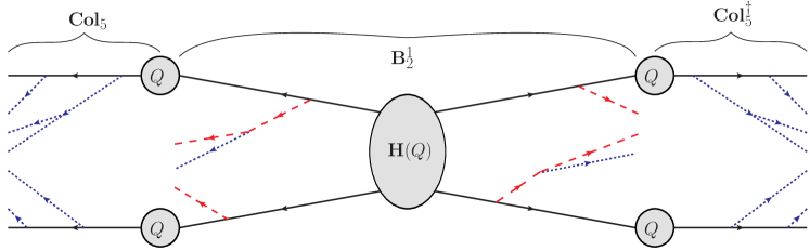
Figure 3: Illustrating hard-leg factorisation. Red dashed lines represent the emission of soft gluons and collinear emissions are represented by blue dotted lines. Circles indicate the hard scale from which subsequent evolution proceeds. Loops (Sudakov factors) have been neglected to avoid clutter.

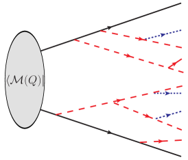
(a) A term contributing to the right evolution ($\mathbf{B}^{3}_{6}$).

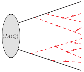
(b) A term contributing to the right evolution ($\mathbf{A}^{\mathrm{soft}}_{9}$).

Figure 4: The right evolution (the evolution of the conjugate amplitude) of a hard process after 9 emissions. Red dashed lines represent the emission of soft gluons and collinear emissions are represented by blue dotted lines. Loops (Sudakov factors) have been neglected to avoid clutter.

The main result of this subsection is the factorisation of collinear physics into jet functions; one for each leg emerging from the hard scatter. We do this with Coulomb gluons removed ($\tilde{\delta}_{ij}=0$) and will discuss their re-introduction in Section 3.3. The following manipulations can equally well be performed using either variant A or B of the algorithm. For concreteness we will use variant B whenever an operator needs to be given an explicit definition. Let us begin by simply stating the result:

$$\Sigma(\mu)=\int\sum_{n}\left(\prod^{n}_{i=1}\mathrm{d}\Pi_{i}\right)\sum^{n}_{m=0}\sum^{n-m}_{p=0}\mathrm{Tr}\,\left(\mathbf{Col}^{\dagger}_{m}(\mu)\circ\mathbf{Col}_{m}(\mu)\,\mathbf{B}^{p}_{n-m-p}(\mu)\right).$$ (64)

Figure 3 illustrates what is going on diagrammatically (it shows a contribution with $n=8$, $m=5$ and $p=1$). The collinear evolution operators for hard legs, which provide an operator description of a jet function, are constructed iteratively according to

$$\begin{split}\mathbf{Col}_{0}(q_{\bot})&=\mathbf{V}^{\mathrm{col}}_{q_{\bot},Q},\\ \mathbf{Col}_{m}(q_{\bot})&=\mathbf{V}^{\mathrm{col}}_{q_{\bot},q_{m\,\bot}}\overline{\mathbf{C}}_{m}\mathbf{Col}_{m-1}(q_{m\,\bot})\,\Theta(q_{\bot}\leq q_{m\,\bot}),\end{split}$$ (65)

where

$$\begin{split}\mathbf{V}^{\mathrm{col}}_{a,b}&=\exp\left[-\frac{\alpha_{s}}{\pi}\sum_{j}\int^{b}_{a}\frac{\mathrm{d}k^{(j\vec{n})}_{\bot}}{k^{(j\vec{n})}_{\bot}}\sum_{\upsilon}\mathbb{T}^{\bar{\upsilon}\,2}_{j}\int\frac{\mathrm{d}z\,\mathrm{d}\phi}{8\pi}\mathcal{P}^{\,\circ}_{\upsilon\upsilon_{j}}\right],\\ \overline{\mathbf{C}}_{i}&=\sum_{j}\frac{q^{(j\vec{n})}_{i\,\bot}}{2\sqrt{z_{i}}}\Delta_{ij}\,\mathbf{P}_{ij}.\end{split}$$ (66)

In both operators $j$ sums only over hard partons. The circle operation, $\circ$, indicates the sharing of partons between $\mathbf{Col}_{m}(\mu)$ and $\mathbf{Col}^{\dagger}_{m}(\mu)$, i.e.

$$\begin{split}\mathbf{Col}_{m}(q_{\bot})\circ\mathbf{Col}^{\dagger}_{m}(q_{\bot})&=\mathbf{V}^{\mathrm{col}}_{q_{\bot},q_{m\,\bot}}\overline{\mathbf{C}}_{m}\,\mathbf{Col}_{m-1}(q_{m\,\bot})\circ\mathbf{Col}^{\dagger}_{m-1}(q_{m\,\bot})\,\overline{\mathbf{C}}^{\dagger}_{m}\mathbf{V}^{\mathrm{col}\,\dagger}_{q_{\bot},q_{m\,\bot}}.\end{split}$$ (67)

$\mathbf{B}^{p}_{n-m-p}(\mu)$ are the scattering matrices evolved using the algorithm, modified so that all collinear emissions from hard legs have been removed. Specifically,

$$\tilde{\mathbf{A}}_{n-m}(\mu)=\sum_{p=0}^{n-1}\mathbf{B}^{p}_{n-p-m}(\mu),$$ (68)

where $\tilde{\mathbf{A}}_{n-m}(\mu)$ is computed using (2) with the collinear evolution off hard legs removed, i.e. with the replacements $\mathbf{D}_{i}\mapsto\mathbf{D}_{i}-\overline{\mathbf{C}}_{i}$ and $\mathbf{V}_{a,b}\mapsto\mathbf{V}_{a,b}(\mathbf{V}^{\mathrm{col}}_{a,b})^{-1}$. The number of collinear emissions not off hard legs is indexed by $p$ and $n-p-m$ is the number of soft emissions (in equation (64), $m$ is the number of collinear emissions off hard legs). An example term, contributing to $\mathbf{B}^{3}_{6}(\mu)$, is presented in Figure 4(a).

It may be helpful to contrast $\mathbf{B}^{p}_{n}(\mu)$ with scattering matrices evolved using the FKS algorithm SoftEvolutionAlgorithm . We denote the FKS matrices as $\mathbf{A}^{\mathrm{soft}}_{n}(\mu)$ and they can be evaluated using variant A with $\overline{\mathcal{P}}_{\upsilon_{i}\upsilon_{j}}=0$; an example is shown in Figure 4(b). Note that $\mathbf{B}^{0}_{n}(\mu)\neq\mathbf{A}^{\mathrm{soft}}_{n}(\mu)$ for $n\geq 1$ since $\mathbf{B}^{0}_{n}(\mu)$ still contains the collinear Sudakov factors ‘attached’ to soft partonic legs. Also note that $\mathbf{B}^{0}_{0}(\mu)=\mathbf{A}^{\mathrm{soft}}_{0}(\mu)$ and $\mathbf{B}^{i}_{0}(\mu)=0$ for all $i>0$. In Section 3.2 we will generalise the arguments presented here so that we can factorise collinear physics into jet functions that multiply $\mathbf{A}^{\mathrm{soft}}_{n}(\mu)$. However, in this section we will not make any further use of $\mathbf{A}^{\mathrm{soft}}_{n}(\mu)$.

Equation (64) can be written more simply by combining the collinear evolution operators (which are proportional to unit operators in colour space) into a single cross-section level jet function, $\mathbf{Col}^{\dagger}_{m}(\mu)\circ\mathbf{Col}_{m}(\mu)=\mathbbm{1}\otimes\mathrm{Col}_{m}(\mu)$. Doing this enables (64) to be written as

$$\Sigma(\mu)|_{u_{n}=1}=\int\sum_{n}\left(\prod^{n}_{i=1}\mathrm{d}\Pi_{i}\right)\sum^{n}_{m=0}\sum^{n-m}_{p=0}\mathrm{Tr}_{s}\left(\mathrm{Col}_{m}(\mu)\,\mathrm{Tr}_{c}\,\mathbf{B}^{p}_{n-m-p}(\mu)\right),$$ (69)

where the traces are over colour, $c$, and helicity, $s$. However, we avoid working with collinear factorisation in this form because it does not apply when Coulomb exchanges are present.

Having stated the result, let us now proceed to show how it is derived. The following commutation relations are important:

$$\begin{split}\left[\mathbf{D}_{i}-\overline{\mathbf{C}}_{i},\overline{\mathbf{C}}_{j}\right]\simeq 0,\qquad\left[\mathbf{V}_{a,b}(\mathbf{V}^{\mathrm{col}}_{a,b})^{-1},\overline{\mathbf{C}}_{j}\right]\simeq 0,\qquad\\ \left[\mathbf{V}_{a,b}(\mathbf{V}^{\mathrm{col}}_{a,b})^{-1},\mathbf{V}^{\mathrm{col}}_{c,d}\right]\simeq 0,\qquad\left[\mathbf{D}_{i}-\overline{\mathbf{C}}_{i},\mathbf{V}^{\mathrm{col}}_{a,b}\right]\simeq 0.\end{split}$$ (70)

Here $\simeq$ denotes equality when the operator acts on a matrix element, which is all we ever encounter.

$[\mathbf{V}_{a,b}(\mathbf{V}^{\mathrm{col}}_{a,b})^{-1},\mathbf{V}^{\mathrm{col}}_{c,d}]\simeq 0$ and $[\mathbf{D}_{i}-\overline{\mathbf{C}}_{i},\mathbf{V}^{\mathrm{col}}_{a,b}]\simeq 0$ are trivial to show as $\mathbf{V}^{\mathrm{col}}_{a,b}$ is proportional to the identity in colour-helicity space. Diagrammatically, proving

$$[\mathbf{V}_{a,b}(\mathbf{V}^{\mathrm{col}}_{a,b})^{-1},\mathbf{V}^{\mathrm{col}}_{c,d}]\simeq 0$$

reduces to showing

$$\begin{split}\begin{array}[]{c}\includegraphics[width=108.405pt]{VV_commutator_1}\end{array}=\begin{array}[]{c}\includegraphics[width=108.405pt]{VV_commutator_2}\end{array},\end{split}$$ (71)

and $[\mathbf{D}_{i}-\overline{\mathbf{C}}_{i},\mathbf{V}^{\mathrm{col}}_{a,b}]\simeq 0$ to showing

$$\begin{split}\begin{array}[]{c}\includegraphics[width=108.405pt]{DV_commutator_1}\end{array}=\begin{array}[]{c}\includegraphics[width=108.405pt]{DV_commutator_2}\end{array}.\end{split}$$ (72)

As ever, a red dashed line is used to represent a soft parton and a blue dotted line represents a collinear parton. The black dashed line indicates a cut (cut lines are on shell).

$[\mathbf{V}_{a,b}(\mathbf{V}^{\mathrm{col}}_{a,b})^{-1},\overline{\mathbf{C}}_{j}]\simeq 0$ and $[\mathbf{D}_{i}-\overline{\mathbf{C}}_{i},\overline{\mathbf{C}}_{j}]\simeq 0$ can be shown by factorising kinematic factors from the colour and helicity operators, then carefully tracking the action of the colour operators so that colour conservation can be applied. Proving the commutators also requires noting that both soft real emissions and soft Sudakov factors are identity operators in helicity space, and that helicity states are orthogonal. $[\mathbf{V}_{a,b}(\mathbf{V}^{\mathrm{col}}_{a,b})^{-1},\overline{\mathbf{C}}_{j}]\simeq 0$ presents the biggest challenge. The derivation follows closely the discussion in SuperleadingLogs . It is most easily illustrated by expressing the operators diagrammatically. Doing so reduces the problem to showing

$$\begin{split}\begin{array}[]{c}\includegraphics[width=108.405pt]{VC_commutator_1}\end{array}&+\begin{array}[]{c}\includegraphics[width=108.405pt]{VC_commutator_2}\end{array}+\begin{array}[]{c}\includegraphics[width=108.405pt]{VC_commutator_3}\end{array}\\ &=\begin{array}[]{c}\includegraphics[width=108.405pt]{VC_commutator_4}\end{array}.\end{split}$$ (73)

Also note that

$$[\mathbf{V}_{a,b}(\mathbf{V}^{\mathrm{col}}_{a,b})^{-1},\overline{\mathbf{C}}_{j}]\simeq 0$$

implies $[\mathbf{D}_{i}-\overline{\mathbf{C}}_{i},\overline{\mathbf{C}}_{j}]\simeq 0$ since

$$\begin{split}\begin{array}[]{c}\includegraphics[width=108.405pt]{DC_commutator_1}\end{array}+\begin{array}[]{c}\includegraphics[width=108.405pt]{DC_commutator_2}\end{array}=\begin{array}[]{c}\includegraphics[width=108.405pt]{DC_commutator_3}\end{array},\end{split}$$ (74)

which trivially follows from (73). Using these commutation relations, reconstructing the separate strong orderings of collinear and soft physics in (64) is simply a case of careful combinatorics and relabelling of momenta. For instance

$$\begin{split}&\left[\begin{array}[]{c}\includegraphics[width=86.72267pt]{DC_commutator_1}\end{array}+\begin{array}[]{c}\includegraphics[width=86.72267pt]{DC_commutator_2}\end{array}\right]\Theta(q_{j\,\bot}-q_{i\,\bot})\Theta(q_{i\,\bot}-\mu)\Theta(Q-q_{j\,\bot})\\ &+\begin{array}[]{c}\includegraphics[width=86.72267pt]{DC_commutator_3}\end{array}\Theta(q_{i\,\bot}-q_{j\,\bot})\Theta(q_{j\,\bot}-\mu)\Theta(Q-q_{i\,\bot})\\ &=\begin{array}[]{c}\includegraphics[width=86.72267pt]{DC_commutator_3}\end{array}\Theta(q_{i\,\bot}-\mu)\Theta(Q-q_{i\,\bot})\Theta(q_{j\,\bot}-\mu)\Theta(Q-q_{j\,\bot}).\end{split}$$ (75)

For the sake of completeness, in the next section we will go ahead and put back $\mathfrak{R}^{\mathrm{soft}}$, $\mathfrak{R}^{\mathrm{coll}}$, and the measurement functions. However, we have only proven correctness at LL accuracy. As such, Sections 3.1.1 and 3.1.2 are conjectures. It might be the case that only certain classes of recoil prescription factorise in this way. We will focus on variant A in Section 3.1.1 and turn to variant B in Section 3.1.2, where we show how to re-instate the plus prescription in the collinear splitting functions. We caution that both these versions of the algorithm will not produce super-leading logarithms because Coulomb interactions have been neglected. Therefore they are only suitable for processes with fewer than two coloured particles in either the initial or final state of the hard process, i.e. $e^{+}e^{-}$, deep-inelastic scattering and Drell-Yan.

3.1.1 The details

Now we summarise the results of the previous section and make a conjecture regarding the inclusion of recoils (recall we left these out of the discussions in the previous section). For concreteness we use variant A. The evolution has two phases. In the first phase soft gluons are emitted:

$$\begin{split}\boldsymbol{\sigma}(0,0)&=\tilde{\mathbf{V}}_{\mu,Q}\mathbf{H}(Q;\{p\})\tilde{\mathbf{V}}^{\dagger}_{\mu,Q}=\tilde{\mathbf{A}}_{0}(\mu;\{p\}),\\ \mathbf{d}\boldsymbol{\sigma}(1,0)&=\int\prod_{i}\mathrm{d}^{4}p_{i}\tilde{\mathbf{V}}_{\mu,q_{1\,\bot}}\tilde{\mathbf{D}}_{1}\tilde{\mathbf{A}}_{0}(q_{1\,\bot};\{p\})\tilde{\mathbf{D}}^{\dagger}_{1}\tilde{\mathbf{V}}^{\dagger}_{\mu,q_{1\,\bot}}\mathrm{d}\Pi_{1}\\ &\;=\tilde{\mathbf{A}}_{1}(\mu;\{p\}_{1})\mathrm{d}\Pi_{1}\equiv\mathbf{B}^{0}_{1}(\mu;\{p\}_{1})\mathrm{d}\Pi_{1},\\ \mathbf{d}\boldsymbol{\sigma}(2,0)&=\int\prod_{i}\mathrm{d}^{4}p_{i}\tilde{\mathbf{V}}_{\mu,q_{2\,\bot}}\tilde{\mathbf{D}}_{2}\tilde{\mathbf{A}}_{1}(q_{2\,\bot};\{p\})\tilde{\mathbf{D}}^{\dagger}_{2}\tilde{\mathbf{V}}^{\dagger}_{\mu,q_{2\,\bot}}\mathrm{d}\Pi_{1}\mathrm{d}\Pi_{2}\\ &\;=\tilde{\mathbf{A}}_{2}(\mu;\{p\}_{2})\mathrm{d}\Pi_{1}\mathrm{d}\Pi_{2}\equiv\left(\mathbf{B}^{0}_{2}(\mu)+\mathbf{B}^{1}_{1}(\mu)\right)\mathrm{d}\Pi_{1}\mathrm{d}\Pi_{2},\\ \mathbf{d}\boldsymbol{\sigma}(n,0)&\;=\tilde{\mathbf{A}}_{n}(\mu;\{p\}_{n})\prod^{n}_{i=1}\mathrm{d}\Pi_{i}\equiv\sum_{p=0}^{n}\mathbf{B}^{p}_{n-p}(\mu)\prod^{n}_{i=1}\mathrm{d}\Pi_{i},\end{split}$$ (76)

where $\tilde{\mathbf{D}}_{i}=\mathbf{D}_{i}-\overline{\mathbf{C}}_{i}$ and

$$\begin{split}\overline{\mathbf{C}}_{i}=\sum_{l}\frac{q^{(l\vec{n})}_{i\,\bot}}{2\sqrt{z_{i}}}\Delta_{il}\,\overline{\mathbf{P}}_{il}\,\mathfrak{R}^{\mathrm{coll}}_{ij}(\{p\},\{\tilde{p}\},q_{i}),\end{split}$$ (77)

where $l$ sums only over hard partons. And $\tilde{\mathbf{V}}_{a,b}=\mathbf{V}_{a,b}(\overline{\mathbf{V}}_{a,b})^{-1}$ and

$$\begin{split}\overline{\mathbf{V}}_{a,b}&=\exp\left[-\frac{\alpha_{s}}{\pi}\sum_{l}\int^{b}_{a}\frac{\mathrm{d}k^{(l\vec{n})}_{\bot}}{k^{(l\vec{n})}_{\bot}}\sum_{\upsilon}\mathbb{T}^{\bar{\upsilon}\,2}_{\bar{l}}\int\frac{\mathrm{d}z\,\mathrm{d}\phi}{8\pi}\,\overline{\mathcal{P}}^{\,\circ}_{\upsilon\upsilon_{l}}\,\mathcal{R}^{\mathrm{coll}}_{l}\right].\end{split}$$ (78)

Again, the sum over $l$ only includes hard partons. In $\mathbf{d}\boldsymbol{\sigma}(n,m)$, $n$ indicates the number of soft emissions, which occur during the first phase of the evolution, and $m$ indicates the number of collinear emissions, which occur during the second phase of the evolution.

The second phase of the evolution dresses the hard legs with collinear emissions:

$$\begin{split}\mathrm{d}\sigma(n,0)&=\mathrm{Tr}\,\left(\overline{\mathbf{V}}_{\mu,Q}\,\mathbf{d}\boldsymbol{\sigma}(n,0)\,\overline{\mathbf{V}}^{\dagger}_{\mu,Q}\right)=\mathrm{Tr}\,(\tilde{\mathbf{A}}^{n}_{n+0}(\mu;\{p\}_{n}))\\ &\equiv\sum_{p=0}^{n}\mathrm{Tr}(\mathbf{Col}^{\dagger}_{0}(\mu)\circ\mathbf{Col}_{0}(\mu)\,\mathbf{B}^{p}_{n-p}(\mu)),\\ \mathrm{d}{\sigma}(n,1)&=\int\prod_{i}\mathrm{d}^{4}p_{i}\,\mathrm{Tr}\,\left(\overline{\mathbf{V}}_{\mu,q_{n+1\,\bot}}\overline{\mathbf{C}}_{n+1}\overline{\mathbf{V}}_{q_{n+1\,\bot},Q}\,\mathbf{d}\boldsymbol{\sigma}(n,0)\right.\\ &\qquad\left.\times\overline{\mathbf{V}}^{\dagger}_{q_{n+1\,\bot},Q}\overline{\mathbf{C}}^{\dagger}_{n+1}\overline{\mathbf{V}}^{\dagger}_{\mu,q_{n+1\,\bot}}\right)\mathrm{d}\Pi_{n+1}=\mathrm{Tr}\,(\tilde{\mathbf{A}}^{n}_{n+1}(\mu;\{p\}_{n+1}))\mathrm{d}\Pi_{n+1}\\ &\equiv\sum_{p=0}^{n}\mathrm{Tr}(\mathbf{Col}^{\dagger}_{1}(\mu)\circ\mathbf{Col}_{1}(\mu)\,\mathbf{B}^{p}_{n-p}(\mu))\mathrm{d}\Pi_{n+1},\\ \mathrm{d}\sigma(n,m)&\;=\;\mathrm{Tr}\,(\tilde{\mathbf{A}}^{n}_{n+m}(\mu;\{p\}_{n+m}))\prod^{m}_{i=1}\mathrm{d}\Pi_{n+i}\\ &\equiv\sum_{p=0}^{n}\mathrm{Tr}(\mathbf{Col}^{\dagger}_{m}(\mu)\circ\mathbf{Col}_{m}(\mu)\,\mathbf{B}^{p}_{n-p}(\mu))\prod^{m}_{i=1}\mathrm{d}\overline{\Pi}_{n+i},\end{split}$$ (79)

where $\tilde{\mathbf{A}}^{n}_{n+m}$ obeys the recurrence relation

$$\begin{split}\tilde{\mathbf{A}}^{n}_{n+m}(q_{\bot};\{\tilde{p}\}_{n+m-1}\cup q_{n+m})&=\int\prod_{i}\mathrm{d}^{4}p_{i}\overline{\mathbf{V}}_{q_{\bot},q_{n+m\,\bot}}\overline{\mathbf{C}}_{n+m}\tilde{\mathbf{A}}^{n}_{n+m-1}(q_{n+m\,\bot};\{p\}_{n+m-1})\\ &\qquad\times\overline{\mathbf{C}}^{\dagger}_{n+m}\overline{\mathbf{V}}^{\dagger}_{q_{\bot},q_{n+m\,\bot}}\Theta(q_{\bot}\leq q_{n+m\,\bot}).\end{split}$$

An observable can be calculated using

$$\Sigma(\mu)=\sum_{n}\int\mathrm{d}\sigma_{n}\,u_{n}(q_{1},...,q_{n}),$$ (80)

where $\mathrm{d}\sigma_{n}=\sum_{m=0}^{n}\mathrm{d}\sigma(n-m,m)$.

3.1.2 Recovering the ‘plus prescription’

Now let us turn to variant B. Recall that, in this variant of the algorithm collinear evolution proceeds using the full DGLAP splitting functions. Things are precisely as in the last subsection except that we now use the splitting operators without overlines ($\mathbf{P}_{il}$) and the functions $\mathfrak{f}$ and $\mathcal{F}$ are to be included in the soft terms. We can go a little further and expand out the Sudakov factors in order to recover the familiar DGLAP plus prescription. To that end, we expand the collinear Sudakov factors ($\overline{\mathbf{V}}$) that appear in the second phase of the evolution:

$$\begin{split}\overline{\mathbf{V}}_{a,b}=&\mathbbm{1}-\int^{b}_{a}\frac{\mathrm{d}k_{1\,\bot}}{k_{1\,\bot}}\Gamma_{1}+\int^{b}_{a}\frac{\mathrm{d}k_{2\,\bot}}{k_{2\,\bot}}\Gamma_{1}\int^{b}_{k_{1}}\frac{\mathrm{d}k_{2\,\bot}}{k_{2\,\bot}}\Gamma_{2}-...\end{split}$$ (81)

where

$$\begin{split}\Gamma_{i}=\frac{\alpha_{s}}{\pi}\sum_{l}\sum_{\upsilon}\mathbb{T}^{\bar{\upsilon}\,2}_{\bar{l}}\int\frac{\mathrm{d}z_{i}\,\mathrm{d}\phi_{i}}{8\pi}\overline{\mathcal{P}}^{\,\circ}_{\upsilon\upsilon_{l}}\,\mathcal{R}^{\mathrm{coll}}_{l}.\end{split}$$ (82)

Once again, the sum over $l$ is only over hard partons. Using this, we can regroup terms in the same way as Section 2.5 to generate the plus prescription:

$$\begin{split}\mathrm{d}{\sigma}(n,0)&=\mathrm{Tr}\,\left(\mathbf{d}\boldsymbol{\sigma}(n,0)\right)=\mathrm{Tr}\,\tilde{\mathbf{A}}^{n}_{n+0},\\ \mathrm{d}{\sigma}(n,1)&=\int\prod_{i}\mathrm{d}^{4}p_{i}\,\mathrm{Tr}\,\left(\overline{\mathbf{D}}_{n+1}\mathbf{d}\boldsymbol{\sigma}(n,0)\,\overline{\mathbf{D}}^{\dagger}_{n+1}\right)\mathrm{d}\overline{\Pi}_{n+1}\\ &\;=\mathrm{Tr}\,\tilde{\mathbf{A}}^{n}_{n+1}(\mu;\{p\}_{n+1})\mathrm{d}\overline{\Pi}_{n+1},\\ \mathrm{d}\sigma(n,m)&\;=\mathrm{Tr}\,\tilde{\mathbf{A}}^{n}_{n+m}(\mu;\{p\}_{n+m})\prod^{m}_{i=1}\mathrm{d}\overline{\Pi}_{n+i}\\ &\equiv\sum_{p=0}^{n}\mathrm{Tr}\left(\left[\mathbf{Col}^{\dagger}_{m}(\mu)\circ\mathbf{Col}_{m}(\mu)+\mathcal{O}(\alpha^{m+1}_{s})\right]\,\mathbf{B}^{p}_{n-p}(\mu)\right)\prod^{m}_{i=1}\mathrm{d}\overline{\Pi}_{n+i},\end{split}$$ (83)

where

$$\begin{split}\tilde{\mathbf{A}}^{n}_{n+m}(q_{\bot};\{\tilde{p}\}_{n+m-1}\cup q_{n+m})&=\overline{\mathbf{D}}_{n+m}\tilde{\mathbf{A}}^{n}_{n+m-1}(q_{n+m\,\bot};\{p\}_{n+m-1})\overline{\mathbf{D}}^{\dagger}_{n+m}\Theta(q_{\bot}\leq q_{n+m\,\bot}),\end{split}$$

using the boundary condition that

$$\tilde{\mathbf{A}}^{n}_{n+1}(q_{\bot})=\overline{\mathbf{D}}_{n+1}\tilde{\mathbf{A}}^{n}_{n+0}\overline{\mathbf{D}}^{\dagger}_{n+1}\Theta(q_{\bot}\leq q_{n+1\,\bot})\Theta(q_{n+1\,\bot}\leq Q),$$ (84)

and

$$\overline{\mathbf{D}}_{i}=\sum_{\bar{l}}\frac{q^{(\bar{l}\vec{n})}_{i\,\bot}}{2}\Delta_{i\bar{l}}\,\mathbf{P}^{+}_{i\bar{l}}\,\mathfrak{R}^{\mathrm{coll}}_{ij}(\{p\},\{\tilde{p}\},q_{i}).$$ (85)

The sum over $\bar{l}$ only includes hard partons. $\mathbf{P}_{il}$ has been redefined to include the plus prescription and labelled $\mathbf{P}^{+}_{i\bar{l}}$. The plus prescription is defined in Appendix A. Observables are computed using (80).

3.2 Complete collinear factorisation without Coulomb interactions

Now we are going to go ahead and factorise the collinear physics completely. Once again, the manipulations are essentially the same for either variant of our algorithm. To be concrete, we will use variant B whenever an exact definition must be given. As before, we will begin by stating the final result:

$$\Sigma(\mu)=\int\sum_{n}\left(\prod^{n}_{i=1}\mathrm{d}\Pi_{i}\right)\sum^{n}_{m=0}\mathrm{Tr}\,\left(\mathbf{tCol}^{\dagger}_{m}(\mu)\circ\mathbf{tCol}_{m}(\mu)\mathbf{A}^{\mathrm{soft}}_{n-m}(\mu)\right),$$ (86)

where have we defined the following operators:

$$\begin{split}\mathbf{tCol}_{0}(q_{\bot})&=\mathbf{V}^{\mathrm{tcol}}_{q_{\bot},Q},\\ \mathbf{tCol}_{m}(q_{\bot})&=\mathbf{V}^{\mathrm{tcol}}_{q_{\bot},q_{m\,\bot}}\tilde{\mathbf{C}}_{m}\,\mathbf{tCol}_{m-1}(q_{m\,\bot})\,\Theta(q_{\bot}\leq q_{m\,\bot}),\\ \mathbf{V}^{\mathrm{tcol}}_{a,b}&=\exp\left[-\frac{\alpha_{s}}{\pi}\sum_{j}\int^{b}_{a}\frac{\mathrm{d}k^{(j\vec{n})}_{\bot}}{k^{(j\vec{n})}_{\bot}}\Theta(q^{(j\vec{n})}_{i\,\bot}\leq p_{j\,\bot})\,\sum_{\upsilon}\mathbb{T}^{\bar{\upsilon}\,2}_{j}\int\frac{\mathrm{d}z\,\mathrm{d}\phi}{8\pi}\mathcal{P}^{\,\circ}_{\upsilon\upsilon_{j}}\right],\\ \tilde{\mathbf{C}}_{i}&=\sum_{j}\frac{q^{(j\vec{n})}_{i\,\bot}}{2\sqrt{z_{i}}}\Delta_{ij}\,\mathbf{P}_{ij}\,\Theta(q^{(j\vec{n})}_{i\,\bot}\leq p_{j\,\bot}),\end{split}$$ (87)

and the index $j$ runs over all partons (hard, collinear and soft). We continue to leave aside the functions $\mathfrak{R}^{\mathrm{soft}}$, $\mathfrak{R}^{\mathrm{coll}}$, from emission operators and Sudakov factors. These can readily be re-instated as in Sections 3.1.1 and 3.1.2. $\mathbf{A}^{\mathrm{soft}}_{n}(\mu)$ is as defined in Section 3.1 and evolves the same as $\mathbf{A}_{n}(\mu)$ except that $\mathbf{C}_{i}\mapsto 0$ and $\mathbf{V}_{a,b}\mapsto\mathbf{V}_{a,b}(\mathbf{V}^{\mathrm{tcol}}_{a,b})^{-1}\equiv\mathbf{V}^{\mathrm{soft}}_{a,b}$, i.e. it corresponds to summing over diagrams such as the one in Figure 4(b). Ignoring the effects of recoil (and Coulomb exchanges) and using variant A, $\mathbf{A}^{\mathrm{soft}}_{n}(\mu)$ corresponds to FKS evolution SoftEvolutionAlgorithm . One of the possible contributions to $\mathbf{tCol}_{4}^{\dagger}$ is represented in Figure 5. In the figure, we have sacrificed the intuitive picture of a parton cascade in lieu of providing more detail on the evolution. To construct Figure 5, we have employed the Casimir structure of $\mathbf{V}^{\mathrm{tcol}}_{a,b}$ to split it apart as

$$\mathbf{V}^{\mathrm{tcol}}_{a,b}=\prod_{j}\mathbf{U}^{j}_{a,b}$$

where

$$\mathbf{U}^{j}_{a,b}=\exp\left[-\frac{\alpha_{s}}{\pi}\int^{b}_{a}\frac{\mathrm{d}k^{(j\vec{n})}_{\bot}}{k^{(j\vec{n})}_{\bot}}\Theta(q^{(j\vec{n})}_{i\,\bot}\leq p_{j\,\bot})\,\sum_{\upsilon}\mathbb{T}^{\bar{\upsilon}\,2}_{j}\int\frac{\mathrm{d}z\,\mathrm{d}\phi}{8\pi}\mathcal{P}^{\,\circ}_{\upsilon\upsilon_{j}}\right],$$ (88)

and the product over $j$ is over all partons. In the figures we will be explicit with the labelling so that it is clear whether $\mathbf{U}^{j}_{a,b}$ is associated with a hard parton (labelled by $Q$), a soft parton or a collinear parton, i.e. $j\in\{Q,1^{\mathrm{soft}},2^{\mathrm{soft}},...,(n-m)^{\mathrm{soft}},1^{\mathrm{coll}},2^{\mathrm{coll}},...,m^{\mathrm{coll}}\}$. Something more in the style of our previous diagrams is illustrated in Figure 6.

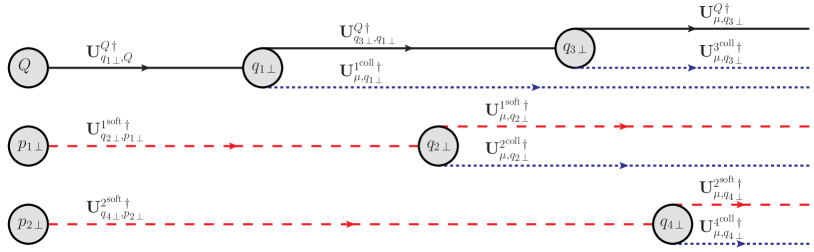
Figure 5: One of the possible contributions to $\mathbf{tCol}_{4}^{\dagger}$. Red dashed lines represent soft gluons and blue dotted lines represent collinear partons. Each line is associated with a Sudakov factor and circles indicate the scale from which the subsequent evolution proceeds. Circles from which two lines leave indicate the action of the operator $\tilde{\mathbf{C}}$. Circles from which one line leaves indicate the scales inherited from the soft evolution phase (not shown). Collinear scales $\{q_{i\,\bot}\}$ are ordered with respect to each other, as are soft scales $\{p_{i\,\bot}\}$. Scales connected along lines are also ordered, with the largest to the left and smallest to the right.

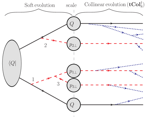
Figure 6: A diagram illustrating factorised parton evolution. Red dashed lines represent the emission of soft gluons and blue dotted lines represent collinear emissions. Circles represent the hard scale from which the subsequent evolution proceeds. Loops (Sudakov factors) have not been drawn.

We will now prove (86) by induction. First, we assume that

$$\mathrm{Tr}\,\mathbf{A}_{n}(\mu)=\sum^{n}_{m=0}\mathrm{Tr}\,\left(\mathbf{tCol}^{\dagger}_{m}(\mu)\circ\mathbf{tCol}_{m}(\mu)\mathbf{A}^{\mathrm{soft}}_{n-m}(\mu)\right),$$ (89)

where $\mathbf{A}_{n}$ is computed as usual from (2). We can see that this is true for $n=1$ by expanding out the $\mathbf{tCol}$ operators and $\mathbf{A}^{\mathrm{soft}}$:

$$\sum^{1}_{m=0}\mathrm{Tr}\,\left(\mathbf{tCol}^{\dagger}_{m}(\mu)\circ\mathbf{tCol}_{m}(\mu)\mathbf{A}^{\mathrm{soft}}_{n-m}(\mu)\right)$$

$$=\mathrm{Tr}\left(\mathbf{V}^{\mathrm{tcol}}_{\mu,q_{1\,\bot}}\tilde{\mathbf{C}}_{1}\mathbf{V}^{\mathrm{tcol}}_{q_{1\,\bot},Q}\mathbf{V}^{\mathrm{soft}}_{\mu,Q}\mathbf{H}(Q)\mathbf{V}^{\mathrm{soft}\,\dagger}_{\mu,Q}\mathbf{V}^{\mathrm{tcol}\,\dagger}_{q_{1\,\bot},Q}\tilde{\mathbf{C}}^{\dagger}_{1}\mathbf{V}^{\mathrm{tcol}\,\dagger}_{\mu,q_{1\,\bot}}\right.$$

$$\qquad\qquad\qquad\left.+\mathbf{V}^{\mathrm{tcol}}_{\mu,Q}\mathbf{V}^{\mathrm{soft}}_{\mu,q_{1\,\bot}}\mathbf{S}_{1}\mathbf{V}^{\mathrm{soft}}_{q_{1\,\bot},Q}\mathbf{H}(Q)\mathbf{V}^{\mathrm{soft}\,\dagger}_{q_{1\,\bot},Q}\mathbf{S}^{\dagger}_{1}\mathbf{V}^{\mathrm{soft}\,\dagger}_{\mu,q_{1\,\bot}}\mathbf{V}^{\mathrm{tcol}\,\dagger}_{\mu,Q}\right)$$

$$=\mathrm{Tr}\left(\mathbf{V}^{\mathrm{soft}}_{\mu,q_{1\,\bot}}\mathbf{V}^{\mathrm{tcol}}_{\mu,q_{1\,\bot}}\mathbf{C}_{1}\mathbf{V}^{\mathrm{tcol}}_{q_{1\,\bot},Q}\mathbf{V}^{\mathrm{soft}}_{q_{1\,\bot},Q}\mathbf{H}(Q)\mathbf{V}^{\mathrm{soft}\,\dagger}_{\mu,Q}\mathbf{V}^{\mathrm{tcol}\,\dagger}_{q_{1\,\bot},Q}\mathbf{C}^{\dagger}_{1}\mathbf{V}^{\mathrm{tcol}\,\dagger}_{\mu,q_{1\,\bot}}\right.$$

$$\qquad\qquad\qquad\left.+\mathbf{U}^{1}_{\mu,q_{1\,\bot}}\mathbf{V}^{\mathrm{col}}_{\mu,q_{1\,\bot}}\mathbf{V}^{\mathrm{soft}}_{\mu,q_{1\,\bot}}\mathbf{S}_{1}\mathbf{V}^{\mathrm{col}}_{q_{1\,\bot},Q}\mathbf{V}^{\mathrm{soft}}_{q_{1\,\bot},Q}\mathbf{H}(Q)\mathbf{V}^{\mathrm{soft}\,\dagger}_{q_{1\,\bot},Q}\mathbf{S}^{\dagger}_{1}\mathbf{V}^{\mathrm{soft}\,\dagger}_{\mu,q_{1\,\bot}}\mathbf{V}^{\mathrm{tcol}\,\dagger}_{\mu,Q}\right)$$

$$=\mathrm{Tr}\left(\mathbf{V}_{\mu,q_{1\,\bot}}\mathbf{D}_{1}\mathbf{V}_{q_{1\,\bot},Q}\mathbf{H}(Q)\mathbf{V}^{\dagger}_{q_{1\,\bot},Q}\mathbf{D}^{\dagger}_{1}\mathbf{V}^{\dagger}_{\mu,q_{1\,\bot}}\right),$$ (90)

where we have used $\tilde{\mathbf{C}}_{1}\equiv\overline{\mathbf{C}}_{1}\equiv\mathbf{C}_{1}$ as it only acts on hard legs. We have also used the commutators $[\mathbf{V}_{a,b}(\mathbf{V}^{\mathrm{col}}_{a,b})^{-1},\mathbf{V}^{\mathrm{col}}_{c,d}]\simeq 0$ and $[\mathbf{V}_{a,b}(\mathbf{V}^{\mathrm{col}}_{a,b})^{-1},\overline{\mathbf{C}}_{j}]\simeq 0$, derived in the previous section, and $\mathbf{V}_{c,a}=\mathbf{V}_{c,b}\mathbf{V}_{b,a}$. Notice in the above expressions the theta functions present in $\tilde{\mathbf{C}}_{1}$ and $\mathbf{V}^{\mathrm{tcol}}_{q_{1\,\bot},Q}$ are always unity on hard legs as the ordering guarantees their argument is satisfied. We will now show that if (89) is true for $\mathbf{A}_{n}$, it is also true for $\mathbf{A}_{n+1}$. We begin by noting that from the Markovian way our algorithm evolves, we can write $\mathbf{A}_{n+1}\equiv\hat{\mathbf{A}}_{n}(\mu,q_{1\,\bot})$ where $\hat{\mathbf{A}}_{n}(\mu,q_{1\,\bot})$ is computed using our algorithm (as described in (2)) however with the evolution initiated by $\hat{\mathbf{H}}(q_{1\,\bot})=\mathbf{D}_{1}\mathbf{V}_{q_{1\,\bot},Q}\mathbf{H}(Q)\mathbf{V}^{\dagger}_{q_{1\,\bot},Q}\mathbf{D}^{\dagger}_{1}$ and with the parton momentum indexed as $2,3,4,...\,$. From this we can use (89) to write

$$\mathrm{Tr}\,\mathbf{A}_{n+1}(\mu)=\mathrm{Tr}\,\hat{\mathbf{A}}_{n}(\mu,q_{1\,\bot})=\sum^{n}_{m=0}\mathrm{Tr}\,\left(\hat{\mathbf{tCol}}^{\dagger}_{m}(\mu,q_{1\,\bot})\circ\hat{\mathbf{tCol}}_{m}(\mu,q_{1\,\bot})\hat{\mathbf{A}}^{\mathrm{soft}}_{n-m}(\mu,q_{1\,\bot})\right),$$ (91)

where $\hat{\mathbf{A}}^{\mathrm{soft}}_{n-m}(\mu,q_{1\,\bot})$ are generated by the same algorithm as $\mathbf{A}^{\mathrm{soft}}_{n-m}(\mu)$ however using $\hat{\mathbf{H}}(q_{1\,\bot})$ as the initial condition. $\hat{\mathbf{tCol}}_{m}(\mu,q_{1\,\bot})$ are generated using the iterative relation in (87) but with an initial condition $\hat{\mathbf{tCol}_{0}}(q_{\bot},q_{1\,\bot})=\mathbf{V}^{\mathrm{tcol}}_{q_{\bot},q_{1\,\bot}}$. Next we split apart $\hat{\mathbf{H}}(q_{1\,\bot})$ as

$$\hat{\mathbf{H}}(q_{1\,\bot})= \mathbf{S}_{1}\mathbf{V}^{\mathrm{tcol}}_{q_{1\,\bot},Q}\mathbf{V}^{\mathrm{soft}}_{q_{1\,\bot},Q}\mathbf{H}(Q)\mathbf{V}^{\mathrm{soft}\,\dagger}_{q_{1\,\bot},Q}\mathbf{V}^{\mathrm{tcol}\,\dagger}_{q_{1\,\bot},Q}\mathbf{S}^{\dagger}_{1}$$

$$+\tilde{\mathbf{C}}_{1}\mathbf{V}^{\mathrm{tcol}}_{q_{1\,\bot},Q}\mathbf{V}^{\mathrm{soft}}_{q_{1\,\bot},Q}\mathbf{H}(Q)\mathbf{V}^{\mathrm{soft}\,\dagger}_{q_{1\,\bot},Q}\mathbf{V}^{\mathrm{tcol}\,\dagger}_{q_{1\,\bot},Q}\tilde{\mathbf{C}}^{\dagger}_{1}.$$ (92)

Using the commutation relations from Section 3.1, we can move the collinear operators in $\hat{\mathbf{H}}(q_{1\,\bot})$ past the soft operators which construct $\hat{\mathbf{A}}^{\mathrm{soft}}_{n-m}(\mu,q_{1\,\bot})$ to arrive at

$$\mathrm{Tr}\,\mathbf{A}_{n+1}(\mu)=\sum^{n}_{m=0}\mathrm{Tr}\,\left(\mathbf{V}^{\mathrm{tcol}\,\dagger}_{q_{1\,\bot},Q}\hat{\mathbf{tCol}}^{\dagger}_{m}(\mu,q_{1\,\bot})\circ\hat{\mathbf{tCol}}_{m}(\mu,q_{1\,\bot})\mathbf{V}^{\mathrm{tcol}}_{q_{1\,\bot},Q}\mathbf{A}^{\mathrm{soft}}_{n+1-m}(\mu,Q)\right)$$

$$+\sum^{n}_{m=0}\mathrm{Tr}\,\left(\mathbf{V}^{\mathrm{tcol}\,\dagger}_{q_{1\,\bot},Q}\tilde{\mathbf{C}}^{\dagger}_{1}\hat{\mathbf{tCol}}^{\dagger}_{m}(\mu,q_{1\,\bot})\circ\hat{\mathbf{tCol}}_{m}(\mu,q_{1\,\bot})\tilde{\mathbf{C}}_{1}\mathbf{V}^{\mathrm{tcol}}_{q_{1\,\bot},Q}\mathbf{A}^{\mathrm{soft}}_{n-m}(\mu,Q)\right).$$ (93)

We can now combine the collinear operators using

$$\hat{\mathbf{tCol}}_{m}(\mu,q_{1\,\bot})\tilde{\mathbf{C}}_{1}\mathbf{V}^{\mathrm{tcol}}_{q_{1\,\bot},Q}=\mathbf{tCol}_{m+1}(\mu)\theta(q^{\mathrm{coll}}_{1\,\bot}>q^{\mathrm{soft}}_{1\,\bot})$$

and

$$\hat{\mathbf{tCol}}_{m}(\mu,q_{1\,\bot})\mathbf{V}^{\mathrm{tcol}}_{q_{1\,\bot},Q}=\mathbf{tCol}_{m}(\mu)\theta(q^{\mathrm{coll}}_{1\,\bot}<q^{\mathrm{soft}}_{1\,\bot}),$$

where in the second equality we need to relabel the momenta of collinear partons again so that they are indexed as $1,2,3,...\,$. We have denoted the momentum of the hardest collinear emission generated by the collinear operators, $\mathbf{tCol}$, as $q^{\mathrm{coll}}_{1}$ and the hardest soft momentum in $\mathbf{A}^{\mathrm{soft}}_{n-m}(\mu,Q)$ as $q^{\mathrm{soft}}_{1}$. Combining the two sums and theta functions, we arrive at

$$\mathrm{Tr}\,\mathbf{A}_{n+1}(\mu)=\sum^{n+1}_{m=0}\mathrm{Tr}\,\left(\mathbf{tCol}^{\dagger}_{m}(\mu)\circ\mathbf{tCol}_{m}(\mu)\mathbf{A}^{\mathrm{soft}}_{n+1-m}(\mu)\right).$$ (94)

Thus we have proven that (86) holds for $n\to n+1$. It is important to note the role of the theta functions in the definitions of $\tilde{\mathbf{C}}_{i}$ and $\mathbf{V}^{\mathrm{tcol}}_{a,b}$. These ensure that the commutation relations from Section 3.1 can always applied. They do this by squeezing to zero the phase space of any collinear partons generated by $\tilde{\mathbf{C}}_{1}$ and $\mathbf{V}^{\mathrm{tcol}}_{q_{1\,\bot},Q}$ from not-hard legs. To illustrate this point, we will consider the relevant Feynman diagrams:

$$\begin{split}&\left[\begin{array}[]{c}\includegraphics[width=86.72267pt]{DC_commutator_1}\end{array}+\begin{array}[]{c}\includegraphics[width=86.72267pt]{DC_commutator_2}\end{array}\right]\Theta(q_{j\,\bot}-q_{i\,\bot})\Theta(q_{i\,\bot}-\mu)\Theta(Q-q_{j\,\bot})\\ &+\left[\begin{array}[]{c}\includegraphics[width=86.72267pt]{DC_commutator_3}\end{array}+\begin{array}[]{c}\includegraphics[width=86.72267pt]{extra_term_1}\end{array}\right]\Theta(q_{i\,\bot}-q_{j\,\bot})\Theta(q_{j\,\bot}-\mu)\Theta(Q-q_{i\,\bot})\\ &=\begin{array}[]{c}\includegraphics[width=86.72267pt]{DC_commutator_3}\end{array}\Theta(q_{i\,\bot}-\mu)\Theta(Q-q_{i\,\bot})\Theta(q_{j\,\bot}-\mu)\Theta(Q-q_{j\,\bot})\\ &+\begin{array}[]{c}\includegraphics[width=86.72267pt]{extra_term_1}\end{array}\Theta(q_{i\,\bot}-q_{j\,\bot})\Theta(q_{j\,\bot}-\mu)\Theta(Q-q_{i\,\bot}).\end{split}$$ (95)

Note that the last term on either side of the equation cannot be manipulated using our commutators and there are no more diagrams we could include which they may cancel against. Nevertheless terms of this form are generated by our algorithm. They represent a collinear parton, emitted from a soft parton, restricted so that its transverse momentum is smaller than the transverse momentum of the soft parton. Using $\tilde{\mathbf{C}}_{i}$, equation (95) reduces to

$$\left\langle\mathcal{M}\right|\mathbf{D}^{\dagger}_{1}\mathbf{D}^{\dagger}_{2}\mathbf{D}_{2}\mathbf{D}_{1}\left|\mathcal{M}\right\rangle\Theta(q_{1\,\bot}-q_{2\,\bot})\Theta(q_{2\,\bot}-\mu)\Theta(Q-q_{1\,\bot})$$

$$=\left\langle\mathcal{M}\right|\mathbf{S}^{\dagger}_{1}\tilde{\mathbf{C}}^{\dagger}_{2}\tilde{\mathbf{C}}_{2}\mathbf{S}_{1}\left|\mathcal{M}\right\rangle\Theta(Q>q_{1\,\bot}>\mu)\Theta(Q>q_{2\,\bot}>\mu).$$ (96)

3.3 Partial collinear factorisation with Coulomb interactions

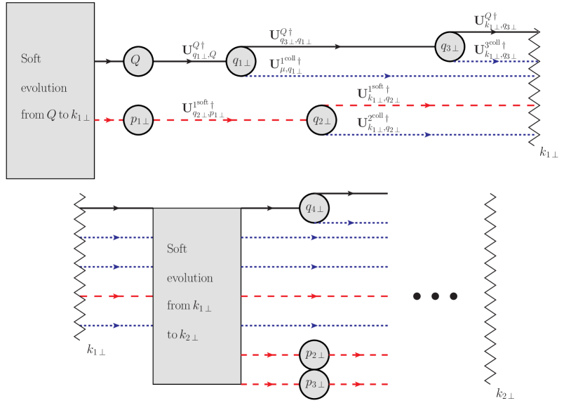
Figure 7: A diagram illustrating factorised parton evolution including Coulomb exchanges. Red dashed lines represent soft gluons and blue dotted lines represent collinear partons. Each line is associated with a Sudakov factor. Circles represent the scale from which the subsequent evolution proceeds. Circles from which two lines leave represent the action of the operator $\tilde{\mathbf{C}}$. Circles from which one line leaves contain the scale information from the preceeding soft evolution. Coulomb exchanges are indicated by vertical zig-zag lines. Momenta are ordered from ‘left to right’, as in Figure 5, including Coulomb exchanges. (The top half of the diagram lies to the ‘left’ of the bottom half.)

Though it is not possible to use the identities in (70) to factorise collinear physics past a Coulomb exchange ($i\pi$ term), it is possible to perform a partial factorisation. Our approach is to expand each Sudakov operator as a series in the number of Coulomb exchanges it resums. Consequently, this enables $\mathbf{A}_{n}$ to be expanded as a series in the number of Coulomb exchanges. We can then factorise soft physics from collinear physics either side of a Coulomb exchange, using our work in the previous section. The partial factorisation is illustrated in Figure 7. We begin by expanding the Sudakov operator:

$$\begin{split}\mathbf{V}_{a,b}=&\hat{\mathbf{V}}_{a,b}-\frac{\alpha_{s}}{\pi}\sum_{i_{1}<j_{1}}\int^{b}_{a}\frac{\mathrm{d}k^{(i_{1}j_{1})}_{1\,\bot}}{k^{(i_{1}j_{1})}_{1\,\bot}}\hat{\mathbf{V}}_{a,k_{1\,\bot}}(\mathbb{T}^{g}_{i_{1}}\cdot\mathbb{T}^{g}_{j_{1}})\,i\pi\,\tilde{\delta}_{i_{1}j_{1}}\hat{\mathbf{V}}_{k_{1\,\bot},b}\\ &+\left(\frac{\alpha_{s}}{\pi}\right)^{2}\sum_{i_{2}<j_{2}}\int^{b}_{a}\frac{\mathrm{d}k^{(i_{1}j_{1})}_{1\,\bot}}{k^{(i_{1}j_{1})}_{1\,\bot}}\sum_{i_{1}<j_{1}}\int_{a}^{k^{(i_{1}j_{1})}_{1\,\bot}}\frac{\mathrm{d}k^{(i_{2}j_{2})}_{2\,\bot}}{k^{(i_{2}j_{2})}_{2\,\bot}}\hat{\mathbf{V}}_{a,k_{2\,\bot}}(\mathbb{T}^{g}_{i_{2}}\cdot\mathbb{T}^{g}_{j_{2}})\,i\pi\,\tilde{\delta}_{i_{2}j_{2}}\\ &\qquad\qquad\times\hat{\mathbf{V}}_{k_{2\,\bot},k_{1\,\bot}}(\mathbb{T}^{g}_{i_{1}}\cdot\mathbb{T}^{g}_{j_{1}})\,i\pi\tilde{\delta}_{i_{1}j_{1}}\hat{\mathbf{V}}_{k_{1\,\bot},b}-...,\end{split}$$ (97)

where $\hat{\mathbf{V}}_{a,b}$ is equal to $\mathbf{V}_{a,b}$ with $\tilde{\delta}_{ij}=0$. Consider using this expanded Sudakov in a parton cascade. The theta functions describing the integral limits on each $i\pi$ term can be used to constrain the limits on the transverse momenta of subsequent emissions (after the $i\pi$). For instance

$$\mathbf{D}_{3}\mathbf{V}_{q_{3\,\bot},q_{2\,\bot}}\mathbf{D}_{2}\mathbf{V}_{q_{2\,\bot},q_{1\,\bot}}\mathbf{D}_{1}$$

$$\quad=...\,+\mathbf{D}_{3}\int^{q_{2\,\bot}}_{q_{3\,\bot}}\frac{\mathrm{d}k_{2\,\bot}}{k_{2\,\bot}}\hat{\mathbf{V}}_{q_{3\,\bot},k_{2\,\bot}}\sum_{i_{2}<j_{2}}(\mathbb{T}^{g}_{i_{2}}\cdot\mathbb{T}^{g}_{j_{2}})\,i\pi\,\hat{\mathbf{V}}_{k_{2\,\bot},q_{2\,\bot}}$$

$$\qquad\qquad\times\mathbf{D}_{2}\int^{q_{1\,\bot}}_{q_{2\,\bot}}\frac{\mathrm{d}k_{1\,\bot}}{k_{1\,\bot}}\hat{\mathbf{V}}_{q_{2\,\bot},k_{1\,\bot}}\sum_{i_{1}<j_{1}}(\mathbb{T}^{g}_{i_{1}}\cdot\mathbb{T}^{g}_{j_{1}})\,i\pi\,\hat{\mathbf{V}}_{k_{1\,\bot},q_{1\,\bot}}\mathbf{D}_{1}+...\,,$$

$$\quad\equiv...\,+\mathbf{D}_{3}\int^{Q}_{\mu}\frac{\mathrm{d}k_{2\,\bot}}{k_{2\,\bot}}\hat{\mathbf{V}}_{q_{3\,\bot},k_{2\,\bot}}\sum_{i_{2}<j_{2}}(\mathbb{T}^{g}_{i_{2}}\cdot\mathbb{T}^{g}_{j_{2}})\,i\pi\,\hat{\mathbf{V}}_{k_{2\,\bot},q_{2\,\bot}}$$

$$\qquad\qquad\times\mathbf{D}_{2}\int^{Q}_{\mu}\frac{\mathrm{d}k_{1\,\bot}}{k_{1\,\bot}}\hat{\mathbf{V}}_{q_{2\,\bot},k_{1\,\bot}}\sum_{i_{1}<j_{1}}(\mathbb{T}^{g}_{i_{1}}\cdot\mathbb{T}^{g}_{j_{1}})\,i\pi\,\hat{\mathbf{V}}_{k_{1\,\bot},q_{1\,\bot}}\mathbf{D}_{1}$$

$$\qquad\qquad\times\Theta(k_{2\,\bot}>q_{3\,\bot})\Theta(k_{1\,\bot}>q_{2\,\bot}>k_{1\,\bot})\Theta(q_{1\,\bot}>k_{1\,\bot})+....\,.$$ (98)

Therefore, we can treat each Coulomb scale as hard relative to the emissions that follow it and soft relative to the emission before it. Thus we can perform a factorised evolution on a hard process up to the scale of the first $i\pi$ term ($k_{1\bot}$). We can take the output from this evolution,

$$\begin{split}\sum_{n}\mathbf{A}_{n}(k_{1\,\bot})=&-\frac{\alpha_{s}}{\pi}\sum_{i_{2}<j_{2}}\frac{\mathrm{d}k^{(i_{1}j_{1})}_{1\,\bot}}{k^{(i_{1}j_{1})}_{1\,\bot}}i\pi\tilde{\delta}_{i_{1}j_{1}}\sum_{n}\sum^{n}_{m=0}\\ &\times\mathrm{Tr}\,\left(\mathbf{A}^{\mathrm{soft}}_{n-m}(k_{1\,\bot})\sum_{i_{1}<j_{1}}\mathbf{Col}^{\dagger}_{m}(k_{1\,\bot})\circ(\mathbb{T}^{g}_{i_{1}}\cdot\mathbb{T}^{g}_{j_{1}})\mathbf{Col}_{m}(k_{1\,\bot})\right),\end{split}$$ (99)

and use it as a new hard process $\mathbf{H}(k_{1\,\bot})$ from which a second factorised evolution can be initiated. This process can be iterated for each $i\pi$ term in the expansion, as illustrated in Figure 7. To complete the computation of $\Sigma$, each $k_{i\,\bot}$ must be integrated over the range $[\mu,Q]$. Interestingly, note that any term in the evolution terminating on a $i\pi$ term to the left of the hard process will cancel against an equivalent term terminating with an $i\pi$ term to the right. Hence collinear emissions can always be factorized below the scale of the last Coulomb exchange. This is consistent with the collinear factorisation shown by Collins, Soper and Sterman Collins:1987pm ; Collins:1988ig .

3.4 Observations on factorisation

Before we leave our discussion on factorisation a few comments are in order. Firstly, we have not been able to achieve factorisation of collinear emissions past Coulomb exchanges. This is to be expected and there is already extensive literature exploring this subject Collins:1988ig ; Mangano:1990by ; BERENDS1988759 ; factorisationBreaking ; Catani:2011st ; SuperleadingLogs ; Rogers:2010dm ; Rogers:2013zha ; Aybat:2008ct . That said, it should be possible to factorise more completely than we have done, by re-expressing the evolution so that all Coulomb terms are only attached to the initial state partons factorisationBreaking , i.e. so we would have complete factorisation on all final state legs.

Secondly, in order to factorise the collinear physics on all legs we had to keep track of intermediate soft scales, from which to initialise the collinear evolution. The number of scales required is equal to the number of soft emissions that occurred prior to factorisation. This means the fully factorised algorithm is no-longer Markovian. We anticipate that our attempts to factorise the collinear physics should bring us in to contact with exact resummations and soft-collinear effective theory (SCET).

It also should be noted that by factorising collinear emissions from the soft evolution, the soft evolution can be explicitly seen to be independent of spin. This is less evident in the interleaved variants of the algorithm. Soft gluons, and subsequent collinear partons, trapped between Coulomb exchanges might conceivably contribute non-trivial spin correlations. This is because, despite equal probabilities for the probability of emission of positive and negative helicity gluons, a collinear emission originating from a soft gluon may depend on its helicity (specifically $g\rightarrow qq$ splitting). This has also been explored in the literature, where it has been noted that soft gluons in the presence of Coulomb/Glauber exchanges can generate spin asymmetries Rogers:2013zha . Further discussions on the spin evolution of the algorithm after factorisation can be found in Appendix B.

It is also interesting to consider the consequences of factorisation in the case of variant B with a universal recoil. A universal recoil allows B to be partitioned in terms of colour-diagonal evolution generated by $\mathbf{C}_{i}$ and colour off-diagonal evolution generated by $\mathbf{S}_{i}$. Hence, provided the recoil prescription does not change the commutators in (70), the proofs of collinear factorisation we have presented become proofs of the complete factorisation of colour-diagonal physics from colour off-diagonal. This is for observables insensitive to the presence of Coulomb exchanges. Since we know that Coulomb exchanges can be factorised onto the initial state factorisationBreaking , this means that there is a complete factorisation of colour-diagonal from colour off-diagonal physics in lepton-lepton, deep-inelastic and Drell-Yan scattering.

Finally, we should remark that it is possible to write down infra-red finite versions of each of the factorised versions of our algorithm, using the procedure in Section 2.5.

4 Phenomenology and resummations

In this section we will first demonstrate how DGLAP evolution emerges. After that, we illustrate the use of the algorithm by calculating thrust, the hemisphere jet mass and gaps-between-jets in $e^{+}e^{-}$.

4.1 DGLAP evolution

We will now show how our algorithm can be used to generate DGLAP evolution, which resums the collinear physics into the running of parton distribution functions. We focus on unpolarised incoming hadrons that collide and produce some high-$p_{T}$ system of interest. We will neglect threshold effects as sub-leading, which is shown carefully in Skands:2009tb ; Nagy:2009re ; Dokshitzer:2008ia . The methods employed in this section can readily be extended to other processes, including those dependent on fragmentation functions.

DGLAP evolution APSplitting ; DOKSHITZER1980269 states that

$$\mu\frac{\partial f_{i}(x,\mu)}{\partial\mu}=\frac{\alpha_{s}}{\pi}\sum_{j}\int^{1}_{x}\frac{\mathrm{d}z}{z}P_{ij}(z)\,f_{j}(x/z,\mu),$$ (100)

where $f_{i}(x,\mu)$ is the parton distribution function for partons of type $i$. $P_{ij}(z)$ are the regularised splitting functions defined at the end of Appendix A. Iterative solutions can be found by expanding the parton distributions:

$$f_{i}(x,Q)=f^{(0)}_{i}(x)+\sum_{n=1}^{\infty}\left(\frac{\alpha_{s}}{\pi}\right)^{n}f^{(n)}_{i}(x,Q),$$ (101)

where $f^{(n)}_{i}(x,\mu)=0$ for all $n\geq 1$. This gives

$$f^{(n+1)}_{i}(x,q_{m-1\,\bot})=\int^{q_{m-1\,\bot}}_{\mu}\frac{\mathrm{d}q_{m\,\bot}}{q_{m\,\bot}}\sum_{j}\int^{1}_{x}\frac{\mathrm{d}z_{m}}{z_{m}}\,P_{ij}(z_{m})f^{(n)}_{j}(x/z_{m},q_{m\,\bot}),$$ (102)

which has a separable solution of the form $f^{(n)}_{i}(x,Q)=f^{(n)}_{i}(x)\frac{1}{n!}\ln^{n}(Q/\mu)$, where $f^{(n)}_{i}(x)$ satisfies

$$f^{(n+1)}_{i}(x)=\sum_{j}\int^{1}_{x}\frac{\mathrm{d}z_{m}}{z_{m}}\,P_{ij}(z_{m})f^{(n)}_{j}(x/z_{m}).$$ (103)

We can write this in terms of the unregularised splitting functions (e.g. see DOKSHITZER1980269 )

$$f^{(n+1)}_{i}(x)=\sum_{j}\int^{1}_{0}\frac{\mathrm{d}z_{m}}{z_{m}}\,\left(\mathcal{P}_{ij}(z_{m})f^{(n)}_{j}(x/z_{m})-z^{2}_{m}\mathcal{P}_{ji}(z_{m})f^{(n)}_{i}(x)\right),$$ (104)

where $f^{(n)}_{j}(x)=0$ for $x>1$ and we have removed factors of $n_{f}$ from $\mathcal{P}_{qg}$.

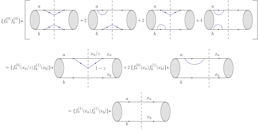
Figure 8: How DGLAP and fragmentation evolution can be constructed from the $\alpha_{s}$ expansion of our algorithm. The vertical dashed lines here correspond to a cut on all external legs (incoming and outgoing) and the grey blobs represent the hard process, i.e. the amplitude evolves from the right grey blob to the vertical dashed line and the conjugate amplitude evolves from the left grey blob to the vertical dashed line. Solid lines indicate hard partons and blue lines collinear partons.

For hadron-hadron collisions, we label the two incoming partons as $a$ and $b$ and their momentum fractions in the hard process as $x_{a}$ and $x_{b}$. We can take the factorised expression corresponding to variant B of our algorithm (64) and attach parton distribution functions:

$$\begin{split}\Sigma=\int\sum_{n}\left(\prod^{n}_{i=1}\mathrm{d}\Pi_{i}\right)\sum^{n}_{m=0}\sum^{n-m}_{p=0}\int\mathrm{d}x_{a}\mathrm{d}x_{b}\,&\mathrm{Tr}\bigg{(}\mathbf{Col}^{\dagger}_{m}(\mu)\circ\mathbf{Col}_{m}(\mu)\\ &\times\mathbf{B}^{p}_{n-m-p}(\mu)\bigg{)}\star\left\{f^{(0)}_{a}(x_{a_{m}})f^{(0)}_{b}(x_{b_{m}})\right\}.\end{split}$$ (105)

$x_{a_{m}}$ and $x_{b_{m}}$ are the momentum fractions of partons $a$ and $b$ respectively after $m$ collinear emissions generated by $\mathbf{Col}^{\dagger}_{m}(\mu)\circ\mathbf{Col}_{m}(\mu)$; they can be related back to $x_{a}$ and $x_{b}$ by momentum conservation along the collinear cascade. The $\star$ operator acts to attach parton distributions of the correct flavour/species to partons $a$ and $b$. There is a technicality relating to parton flavour. That is because DGLAP evolution cares about quark flavour whilst we have defined the splitting operators to sum over quark flavours (in the case $g\to q\bar{q}$). We could have avoided this technicality by defining the splitting operators per flavour (i.e. set $n_{f}=1$ throughout Appendix A). Then we would have to sum over quark flavours throughout the rest of the paper. Instead, we choose to handle quark flavour by keeping track of flavour along the evolution chain, and whenever a $g\to q\bar{q}$ splitting occurs we label the subsequent parton flavour generically, i.e. for two-flavours the relevant set of parton flavours would be $\{u,\bar{u},d,\bar{d},q,g\}$. Note that since we evolve away from the hard scattering, a $g\to q\bar{q}$ branching from an incoming $g$ actually corresponds to a $q\to qg$ (or $\bar{q}\to\bar{q}g$) splitting in the usual DGLAP sense. This can be seen in (A), where the terms involving $\delta^{\text{initial}}_{j}$ and $s_{j}=\pm 1$ involve the $\mathcal{P}_{gq}$ splitting function (the $\mathcal{P}_{qg}$ splitting function appears in the corresponding $\delta^{\text{initial}}$ terms). With this in mind we have that

$$\mathrm{d}\sigma\,\star\left\{f^{A}\,f^{B}\right\}=\sum_{\alpha,\beta}\mathrm{d}\sigma_{\alpha,\beta}\,f^{A}_{\alpha}\,f^{B}_{\beta},$$ (106)

where $\alpha$ and $\beta$ label parton type. For $n_{f}=2$, we would have $\alpha,\beta\in\{u,\bar{u},d,\bar{d},q,g\}$, and $2n_{f}f_{q}$ is the singlet distribution function, i.e. $f_{q}=(u+\bar{u}+d+\bar{d})/(2n_{f})$ for $n_{f}=2$. For completeness, we here also attach labels $A$ and $B$ to indicate the type of hadron (we will drop that label elsewhere in this section).

After expanding $\mathbf{Col}^{\dagger}_{m}(\mu)\circ\mathbf{Col}_{m}(\mu)$ in powers of $\alpha_{s}$, then spin averaging at every vertex, substituting for (103) and evaluating the transverse momentum integrals, we find

$$\begin{split}\Sigma=&\int\sum_{n}\sum^{n}_{m=0}\sum^{n-m}_{p=0}\left(\prod^{n-m}_{i=1}\mathrm{d}\Pi_{i}\right)\\ &\times\int\mathrm{d}x_{a}\mathrm{d}x_{b}\,\mathrm{Tr}\left(\mathbf{B}^{p}_{n-m-p}(\mu)\right)\star\left\{f_{a}(x_{a},Q)f_{b}(x_{b},Q)+\mathcal{O}(\alpha^{m+1}_{s})\right\}.\end{split}$$ (107)

Figure 8 illustrates how terms in our algorithm should be grouped in order to generate the iterative relation in (104) and so arrive at (107). Hence we see that variant B iteratively generates DGLAP evolution up to the hard scale. The derivation of fragmentation function evolution of final-state partons proceeds similarly.

For processes where Coulomb exchanges are relevant, DGLAP evolution is generated up to the scale of the last Coulomb exchange. Also note that, in the infra-red finite reformulations of A and B, DGLAP can be found in the $\mathbf{B}_{n}$ for $n\geq 1$.

4.2 Some familiar resummations

In this subsection we show how to resum a number of observables in $e^{+}e^{-}\rightarrow\mathrm{hadrons}$. The idea is to use well-known results to illustrate the use of the algorithm. The simplicity of the hard process means we can use $\mathbf{H}(Q)=N^{-1}_{c}\sigma_{\mathrm{H}}\mathbbm{1}$ for the hard-scattering matrix. We perform all calculations using the LL recoil from Section 2.4.1.

4.2.1 Thrust

The resummed thrust distribution was initially computed at LL accuracy in Binetruy:1980hd , then at NLL in Resum_large_logs_ee . The current state-of-the-art computation is at $\mathrm{N}^{3}$LL Becher:2008cf . Thrust is defined as

$$T=\max_{\mathbf{n}}\frac{\sum_{\forall\mathbf{p}}|\mathbf{p}\cdot\mathbf{n}|}{\sum_{\forall\mathbf{p}}|\mathbf{p}|},$$ (108)

where the thrust axis $\mathbf{n}$ points along the initial hard parton axis at leading-order in the soft and collinear limits; see Section 3.1 in Resum_large_logs_ee . We will only need to define thrust for 3 partons; of which 2 are hard ($p_{1}$ and $p_{2}$) and one is soft ($k$). We can work in the dipole zero-momentum frame using $p_{q}=E_{q}(1,0,0,1)$, $p_{\bar{q}}=E_{\bar{q}}(1,0,0,-1)$, $k=(k_{\bot}\cosh y,\vec{k}_{\bot},k_{\bot}\sinh y)$, and we can fix $2E_{q}=2E_{\bar{q}}=Q$. Thrust is evaluated as

$$T=1-\frac{k_{\bot}\cosh|y|-k_{\bot}\sinh|y|}{Q}+\mathcal{O}\left(\frac{k^{2}_{\bot}}{Q^{2}}\right).$$ (109)

When calculated in the hard-collinear limit, we can let $T=1+\mathcal{O}(k^{2}_{\bot})$ as all partons lie on the thrust axis up to sub-leading contributions. The thrust distribution $R_{T}$ is defined as

$$R_{T}=\int\mathrm{d}T^{\prime}\frac{1}{\mathrm{Tr}(\mathbf{H}(Q))}\dfrac{\mathrm{d}\Sigma}{\mathrm{d}T^{\prime}}.$$ (110)

As thrust is global, the calculation is most readily performed using the manifestly infra-red finite version of variant A (see Section 2.5). Using this, all terms with one or more emissions cancel exactly. The measurement function $u(k,\{\emptyset\})$ is

$$u(k,\{\emptyset\})=\Theta\left(1-\frac{k^{(q\bar{q})}_{\bot}\cosh|y|-k^{(q\bar{q})}_{\bot}\sinh|y|}{Q}-T\right).$$ (111)

This is unity for a hard-collinear emission, since $|y|\rightarrow\infty$ at LL accuracy. This kills the hard-collinear terms, since they contain a factor $(1-u(k,\{\emptyset\}))=0$, which is as expected since they contribute no double logarithms. Thus we can immediately write

$$\begin{split}\Sigma(T)&=\mathrm{Tr}(\overline{\mathbf{V}}_{0,Q}\overline{\mathbf{V}}^{\dagger}_{0,Q})\sigma_{\mathrm{H}}\\ &=\mathrm{Tr}\left(\exp\left[\frac{2\alpha_{s}}{\pi}\mathbb{T}^{g}_{q}\cdot\mathbb{T}^{g}_{\bar{q}}\int^{Q}_{0}\frac{\mathrm{d}k^{(q\bar{q})}_{\bot}}{k^{(q\bar{q})}_{\bot}}\int\frac{\mathrm{d}S_{2}}{4\pi}\theta_{ij}(k)\right.\right.\\ &\qquad\left.\left.\times\Theta\left(T-1+\frac{k^{(q\bar{q})}_{\bot}\cosh|y|-k^{(q\bar{q})}_{\bot}\sinh|y|}{Q}\right)k_{\bot}^{2}\frac{p_{q}\cdot p_{\bar{q}}}{(p_{q}\cdot k)(p_{\bar{q}}\cdot k)}\right]\right)N^{-1}_{c}\sigma_{\mathrm{H}}.\end{split}$$ (112)

After integrating

$$\begin{split}\Sigma(T)&=\mathrm{Tr}\left(\exp\left[\frac{2\alpha_{s}}{\pi}\mathbb{T}^{g}_{q}\cdot\mathbb{T}^{g}_{\bar{q}}\int^{Q}_{0}\frac{\mathrm{d}k^{(q\bar{q})}_{\bot}}{k^{(q\bar{q})}_{\bot}}2\int^{\infty}_{0}\mathrm{d}y\,\theta_{ij}(k)\Theta\left(\tfrac{k_{\bot}}{Q}e^{-y}-(1-T)\right)\right]\right)N^{-1}_{c}\sigma_{\mathrm{H}},\\ &=\mathrm{Tr}\left(\exp\left[\frac{\alpha_{s}}{\pi}\mathbb{T}^{g}_{q}\cdot\mathbb{T}^{g}_{\bar{q}}\ln^{2}\left(\frac{1}{1-T}\right)\right]\right)N^{-1}_{c}\sigma_{\mathrm{H}}.\end{split}$$ (113)

Here we used the fact that $\theta_{ij}(k)$ restricts the integration so that $k_{0}<Q$. The colour trace can be evaluated to give

$$\begin{split}\frac{\Sigma(T)}{N^{-1}_{c}\sigma_{\mathrm{H}}}&=\mathrm{Tr}(\mathbbm{1})+\frac{\alpha_{s}}{\pi}\ln^{2}\left(\frac{1}{1-T}\right)\mathrm{Tr}\left(\mathbb{T}^{g}_{q}\cdot\mathbb{T}^{g}_{\bar{q}}\right)\\ &\qquad+\frac{1}{2!}\left[\frac{\alpha_{s}}{\pi}\ln^{2}\left(\frac{1}{1-T}\right)\right]^{2}\mathrm{Tr}\left(\mathbb{T}^{g}_{q}\cdot\mathbb{T}^{g}_{\bar{q}}\mathbb{T}^{g}_{q}\cdot\mathbb{T}^{g}_{\bar{q}}\right)+...\\ &=\mathrm{Tr}(\mathbbm{1})-\frac{\alpha_{s}}{\pi}\ln^{2}\left(\frac{1}{1-T}\right)\mathrm{Tr}\left(\mathbb{T}^{g}_{q}\cdot\mathbb{T}^{g}_{q}\right)\\ &\qquad+\frac{1}{2!}\left[\frac{\alpha_{s}}{\pi}\ln^{2}\left(\frac{1}{1-T}\right)\right]^{2}\mathrm{Tr}\left(\mathbb{T}^{g}_{q}\cdot\mathbb{T}^{g}_{q}\mathbb{T}^{g}_{q}\cdot\mathbb{T}^{g}_{q}\right)+...\\ &=\mathrm{Tr}(\mathbbm{1})-\frac{\alpha_{s}}{\pi}\mathcal{C}_{\mathrm{F}}\ln^{2}\left(\frac{1}{1-T}\right)\mathrm{Tr}(\mathbbm{1})+\left[\frac{\alpha_{s}}{\pi}\mathcal{C}^{2}_{\mathrm{F}}\ln^{2}\left(\frac{1}{1-T}\right)\right]^{2}\mathrm{Tr}(\mathbbm{1})+...\\ &=N_{\mathrm{c}}\exp\left[-\frac{\alpha_{s}}{\pi}\mathcal{C}_{\mathrm{F}}\ln^{2}\left(\frac{1}{1-T}\right)\right].\end{split}$$ (114)

And so we obtain the familiar result:

$$\begin{split}R_{T}&=\int\mathrm{d}T^{\prime}\frac{1}{\mathrm{Tr}(\mathbf{H}(Q))}\dfrac{\mathrm{d}\Sigma}{\mathrm{d}T^{\prime}}\\ &=-\frac{\alpha_{s}}{\pi}\mathcal{C}_{\mathrm{F}}\int\mathrm{d}T^{\prime}\,\frac{\ln\left(1-T^{\prime}\right)}{1-T^{\prime}}\exp\left[-\frac{\alpha_{s}}{\pi}\mathcal{C}_{\mathrm{F}}\ln^{2}\left(\frac{1}{1-T^{\prime}}\right)\right].\end{split}$$ (115)

4.2.2 Hemisphere jet mass

The hemisphere jet mass is subject to non-global logarithms, which greatly increase the challenge of resummation. It was first resummed at LL and LC in Dasgupta:2001sh . The current state-of-the-art is split between fixed-order computation ($\alpha^{5}_{s}$ with leading colour Schwartz:2014wha and $\alpha^{4}_{s}$ with full colour Khelifa-Kerfa:2015mma ) and resummation using numerical techniques to introduce full colour dependence with sub-leading logarithms Hagiwara:2015bia . The measurement function corresponding to the hemisphere jet mass in $e^{+}e^{-}\rightarrow\mathrm{hadrons}$ is

$$u_{\pm}(\{q_{i}\})=\prod_{q\in\{q_{i}\}}\left(\Theta(q\in S^{\mp}_{2})+\Theta(q\in S^{\pm}_{2})\Theta(\rho-m_{\pm})\right),$$ (116)

where $S^{+}_{2}$ and $S^{-}_{2}$ are the hemispheres centred on the two primary jets. $m_{\pm}$ is the total invariant mass in the $S^{\pm}_{2}$ hemisphere. The measurement function can be simplified by considering $m_{\pm}$

$$m_{\pm}^{2}=\sum_{q_{i},q_{j}\in S^{\pm}_{2}}2q_{i}\cdot q_{j}=\sum_{q_{i},q_{j}\in S^{\pm}_{2}}2E_{i}E_{j}\left(1-\sqrt{1-\frac{q^{2}_{i\,\bot}}{E^{2}_{i}}}\,\right).$$ (117)

At the order we will perform the calculation we only need to consider one emission, hence

$$\begin{split}u_{\pm}(q_{1})=\Theta(q_{1}\in S^{\mp}_{2})+\Theta(q_{1}\in S^{\pm}_{2})\Theta\left(\rho^{2}-2E_{1}E_{\pm}+2E_{1}E_{\pm}\sqrt{1-q^{2}_{1\,\bot}/E^{2}_{1}}\right),\\ =\left\{\begin{array}[]{ll}\Theta(q_{1}\in S^{\mp}_{2})+\Theta(q_{1}\in S^{\pm}_{2})\Theta\left(\rho^{2}-Q(q_{1\,\bot}\cosh y-q_{1\,\bot}\sinh y)\right)&\;\mathrm{for}\,E_{1}\ll E_{\pm},\\ \Theta(q_{1}\in S^{\mp}_{2})+\Theta(q_{1}\in S^{\pm}_{2})\Theta\left(\rho^{2}-\frac{E_{\pm}}{E_{1}}q^{2}_{1\,\bot})\right)&\;\mathrm{for}\,q_{1\,\bot}\ll E_{1},\end{array}\right.\end{split}$$ (118)

where $E_{\pm}$ is the energy of the quark/anti-quark defining the $S^{\pm}_{2}$ hemisphere and $Q=2E_{\pm}$. Note the similarity between this and the measurement function for thrust, which is expected since it is well known that, at lowest-order, thrust can be expressed as the sum over the two hemisphere jet masses defined by the thrust axis.

Again, we can use the manifestly infra-red finite version of A to find $\Sigma(\rho)$:

$$\begin{split}\Sigma(\rho)=&\mathrm{Tr}(\overline{\mathbf{V}}_{0,Q}\overline{\mathbf{V}}^{\dagger}_{0,Q})N^{-1}_{c}\sigma_{\mathrm{H}}+\int\mathrm{d}\Pi_{1}\mathrm{Tr}\left[\overline{\mathbf{V}}_{0,q_{1\,\bot}}\mathbf{D}_{1}\overline{\mathbf{V}}_{q_{1\,\bot},Q}\overline{\mathbf{V}}^{\dagger}_{q_{1\,\bot},Q}\mathbf{D}^{\dagger}_{1}\overline{\mathbf{V}}^{\dagger}_{0,q_{1\,\bot}}u(q_{1})\right.\\ &\left.\quad\overline{\mathbf{V}}_{0,q_{1\,\bot}}\left\{\overline{\mathbf{V}}_{q_{1\,\bot},Q}\overline{\mathbf{V}}^{\dagger}_{q_{1\,\bot},Q},\frac{1}{2}\mathbf{D}^{2}_{1}\right\}\overline{\mathbf{V}}^{\dagger}_{0,q_{1\,\bot}}u(q_{1},\{\emptyset\})\right]\Theta(Q-q_{1\,\bot})N^{-1}_{c}\sigma_{\mathrm{H}}+...\end{split}$$ (119)

From the calculation in the previous section, we can immediately write

$$\begin{split}\mathrm{Tr}(\overline{\mathbf{V}}_{0,Q}\overline{\mathbf{V}}^{\dagger}_{0,Q})=N_{\mathrm{c}}\exp\left[-\frac{2\alpha_{s}}{\pi}\mathcal{C}_{\mathrm{F}}\ln^{2}\left(\frac{Q}{\rho}\right)\right].\end{split}$$ (120)

This gives the global contribution. The non-global contributions are found by evaluating the remaining terms (corresponding to summing over real emissions in (61)). This calculation can be found in SoftEvolutionAlgorithm , where the non-global terms are evaluated using the FKS algorithm, which is entirely sufficient in this case. Hence we find

$$\begin{split}\Sigma(\rho)=&\sigma_{\mathrm{H}}\exp\left[-\frac{2\alpha_{s}}{\pi}\mathcal{C}_{\mathrm{F}}\ln^{2}\left(Q/\rho\right)\right]\left(1-\mathcal{C}_{\mathrm{A}}\mathcal{C}_{\mathrm{F}}\zeta(2)\left(\frac{\alpha_{s}}{\pi}\right)^{2}\frac{\ln(Q/\rho)^{2}}{2}\right.\\ &\left.-\mathcal{C}^{2}_{\mathrm{A}}\mathcal{C}_{\mathrm{F}}\zeta(3)\left(\frac{\alpha_{s}}{\pi}\right)^{3}\frac{\ln(Q/\rho)^{3}}{3!}+...\right).\end{split}$$ (121)

4.2.3 Gaps-between-jets

The LL measurement function in the case of gaps-between-jets is

$$u_{n}(q_{1},..,q_{n})=\prod_{m=1}^{n}(\Theta_{\mathrm{out}}(q_{m})+\Theta_{\mathrm{in}}(q_{m})\Theta(Q_{0}-q_{m,\bot})),$$ (122)

where the ‘in’ region corresponds to two cones centred on the two leading jets and the ‘out’ region is the region between these cones. The observable vetoes emissions in the out region that have transverse momentum greater than $Q_{0}$. At order $\alpha^{5}_{s}$ this observable is sensitive to super-leading logarithms Forshaw:2006fk ; SuperleadingLogs . These will be correctly calculated using variants A, B and their manifestly infra-red finite versions, but not their factorised form unless Coulomb exchanges are interleaved as in Section 3.3). Using the manifestly infra-red finite version of variant A we correctly find that

$$\begin{split}\Sigma(\mu)&=\sigma_{\mathrm{H}}\exp\left[-\frac{2\alpha_{s}\mathcal{C}_{\mathrm{F}}}{\pi}Y\ln(Q/Q_{0})\right]\left(1+\mathcal{O}(\alpha^{2}_{s})\right),\end{split}$$ (123)

where $Y$ is the rapidity range of the out region and the $\left(1+\mathcal{O}(\alpha^{2}_{s})\right)$ factor is the stack of non-global logarithms, which can be computed by considering real gluon emission into the out region, as encoded in (61). These were calculated up to $\mathcal{O}(\alpha^{5}_{s})$ in SuperleadingLogs ; Forshaw:2006fk ; Keates:2009dn . We note a kinematic maximum on the rapidity of an emitted gluon, i.e. $2|y|<Y_{\mathrm{max}}=\ln\left(\frac{Q}{2Q_{0}}+\sqrt{\frac{Q}{2Q_{0}}-1}\right)$. This means that as $Y\to Y_{\mathrm{max}}$ all soft radiation goes into the in region. At leading-order in the soft approximation $Y_{\mathrm{max}}=\ln(Q/Q_{0})$, i.e. for $Y\geq Y_{\text{max}}$ the observable becomes doubly logarithmic.

5 Conclusions

Our primary goal in writing this paper is to provide the theoretical basis for the future development of a computer code that is able systematically to resum enhanced logarithms due to soft and/or collinear partons including quantum mechanical interference effects. The algorithm we present, and its variants, are (mostly) Markovian and their recursive nature makes them well suited for the task. First steps towards this goal are under development, using the CVolver code to perform the colour evolution Platzer:2013fha ; QCDTalks ; HARPSTalks .

The algorithms in this paper correctly account for the leading soft and/or collinear logarithms, though we have been careful to try and present them in such a way as to make the extension beyond LL possible. For example, we have taken account of the momentum re-mappings that are necessary in order to account for energy-momentum conservation and we have included $g\rightarrow q\bar{q}$ transitions which are strictly single logarithmic.

6 Acknowledgments

This work has received funding from the UK Science and Technology Facilities Council (grant no. ST/P000800/1), the European Union’s Horizon 2020 research and innovation programme as part of the Marie Skłodowska-Curie Innovative Training Network MCnetITN3 (grant agreement no. 722104). JRF thanks the Institute for Particle Physics Phenomenology in Durham for the award of an Associateship and the Particle Physics Group of the University of Vienna for financial support and kind hospitality. JH thanks the UK Science and Technology Facilities Council for the award of a studentship. SP acknowledges partial support by the COST actions CA16201 PARTICLEFACE and CA16108 VBSCAN. We would like to thank Matthew De Angelis for extensive discussions. We would also like to thank Mrinal Dasgupta, Jack Helliwell and Mike Seymour for helpful discussions and comments on the manuscript. Figures have been prepared using JaxoDraw JaxoDraw .

Appendix A Splitting functions

The splitting operator $\mathbf{P}_{ij}$ (see Figure 2), which is explicitly used in variant B of our algorithm, is built from the spin dependent DGLAP splitting functions HelicitySplitting ; HelicitySplitting2 . It is an operator in colour and helicity spaces and is defined using the spinor-helicity formalism HelicityTechniques . We use the convention $v(p,\lambda)=C\bar{u}^{\mathrm{T}}(p,\lambda)$ where $C=i\gamma^{2}\gamma^{0}$, which defines our crossing symmetry to have no global minus sign. Using rotational symmetry and parity invariance one generally can write $\mathcal{M}(\{\lambda_{i}\})=\mathcal{M}^{*}(\{-\lambda_{i}\})$ where $\mathcal{M}$ is a matrix element and $\{\lambda_{i}\}$ the set of helicity states on which $\mathcal{M}$ depends. Together these define the correct treatment for antiparticles, which should evolve as if they are particles with the opposite helicity. Thus $\mathbf{P}_{ij}$ is

$$\begin{split}\mathbf{P}_{ij}&=\delta_{s_{j},\frac{1}{2}}\delta^{\mathrm{final}}_{j}\left(\sqrt{\frac{\mathcal{P}_{qq}}{2\mathcal{C}_{\mathrm{F}}(1+z_{i}^{2})}}\frac{1}{\left\langle q_{i}\tilde{p}_{j}\right\rangle}(\mathbb{T}^{g}_{j}\otimes\mathbb{S}^{+1_{i}})+\sqrt{\frac{z_{i}^{2}\mathcal{P}_{qq}}{2\mathcal{C}_{\mathrm{F}}(1+z_{i}^{2})}}\frac{1}{[\tilde{p}_{j}q_{i}]}(\mathbb{T}^{g}_{j}\otimes\mathbb{S}^{-1_{i}})\right.\\ &\qquad+\sqrt{\frac{\mathcal{P}_{gq}}{2\mathcal{C}_{\mathrm{F}}(2-2z_{i}+z_{i}^{2})}}\frac{1}{\left\langle\tilde{p}_{j}q_{i}\right\rangle}\mathbb{W}^{ij}(\mathbb{T}^{g}_{j}\otimes\mathbb{S}^{+1_{i}})\left.+\sqrt{\frac{(1-z_{i})^{2}\mathcal{P}_{gq}}{2\mathcal{C}_{\mathrm{F}}(2-2z_{i}+z_{i}^{2})}}\frac{1}{[q_{i}\tilde{p}_{j}]}\mathbb{W}^{ij}(\mathbb{T}^{g}_{j}\otimes\mathbb{S}^{-1_{i}})\right)\\ &+\delta_{s_{j},-\frac{1}{2}}\delta^{\mathrm{final}}_{j}\left(\sqrt{\frac{\mathcal{P}_{qq}}{2\mathcal{C}_{\mathrm{F}}(1+z_{i}^{2})}}\frac{1}{[\tilde{p}_{j}q_{i}]}(\mathbb{T}^{g}_{j}\otimes\mathbb{S}^{-1_{i}})+\sqrt{\frac{z_{i}^{2}\mathcal{P}_{qq}}{2\mathcal{C}_{\mathrm{F}}(1+z_{i}^{2})}}\frac{1}{\left\langle q_{i}\tilde{p}_{j}\right\rangle}(\mathbb{T}^{g}_{j}\otimes\mathbb{S}^{+1_{i}})\right.\\ &\qquad+\sqrt{\frac{\mathcal{P}_{gq}}{2\mathcal{C}_{\mathrm{F}}(2-2z_{i}+z_{i}^{2})}}\frac{1}{[q_{i}\tilde{p}_{j}]}\mathbb{W}^{ij}(\mathbb{T}^{g}_{j}\otimes\mathbb{S}^{-1_{i}})\left.+\sqrt{\frac{(1-z_{i})^{2}\mathcal{P}_{gq}}{2\mathcal{C}_{\mathrm{F}}(2-2z_{i}+z_{i}^{2})}}\frac{1}{\left\langle\tilde{p}_{j}q_{i}\right\rangle}\mathbb{W}^{ij}(\mathbb{T}^{g}_{j}\otimes\mathbb{S}^{+1_{i}})\right)\\ &+\delta_{s_{j},1}\delta^{\mathrm{final}}_{j}\left(\sqrt{\frac{(1-z_{i})^{2}\mathcal{P}_{qg}}{2T_{\mathrm{R}}(1-2z_{i}(1-z_{i}))}}\frac{1}{[\tilde{p}_{j}q_{i}]}(\mathbb{W}^{ij}-\mathbbm{1})(\mathbb{T}^{q}_{j}\otimes\mathbb{P}^{1}_{j}\mathbb{P}^{2}_{j}\mathbb{S}^{+\frac{1}{2}_{i}})\right.\\ &\qquad+\sqrt{\frac{z_{i}^{2}\mathcal{P}_{qg}}{2T_{\mathrm{R}}(1-2z_{i}(1-z_{i}))}}\frac{1}{[\tilde{p}_{j}q_{i}]}(\mathbb{W}^{ij}-\mathbbm{1})(\mathbb{T}^{q}_{j}\otimes\mathbb{P}^{2}_{j}\mathbb{S}^{-\frac{1}{2}_{i}})\\ &\qquad+\sqrt{\frac{\mathcal{P}_{gg}}{2\mathcal{C}_{\mathrm{A}}(1-z_{i}+z_{i}^{2})^{2}}}\frac{1}{\left\langle q_{i}\tilde{p}_{j}\right\rangle}(\mathbb{T}^{g}_{j}\otimes\mathbb{S}^{+1_{i}})\\ &\qquad+\sqrt{\frac{z_{i}^{4}\mathcal{P}_{gg}}{2\mathcal{C}_{\mathrm{A}}(1-z_{i}+z_{i}^{2})^{2}}}\frac{1}{[q_{i}\tilde{p}_{j}]}(\mathbb{T}^{g}_{j}\otimes\mathbb{S}^{-1_{i}})\left.+\sqrt{\frac{\mathcal{P}_{gg}(1-z_{i})^{4}}{2\mathcal{C}_{\mathrm{A}}(1-z_{i}+z_{i}^{2})^{2}}}\frac{1}{[\tilde{p}_{j}q_{i}]}(\mathbb{T}^{g}_{j}\otimes\mathbb{P}^{1}_{j}\mathbb{S}^{+1_{i}})\right)\\ &+\delta_{s_{j},-1}\delta^{\mathrm{final}}_{j}\left(\sqrt{\frac{(1-z_{i})^{2}\mathcal{P}_{qg}}{2T_{\mathrm{R}}(1-2z_{i}(1-z_{i}))}}\frac{1}{\left\langle q_{i}\tilde{p}_{j}\right\rangle}(\mathbb{W}^{ij}-\mathbbm{1})(\mathbb{T}^{q}_{j}\otimes\mathbb{P}^{1}_{j}\mathbb{P}^{2}_{j}\mathbb{S}^{-\frac{1}{2}_{i}})\right.\\ &\qquad+\sqrt{\frac{z_{i}^{2}\mathcal{P}_{qg}}{2T_{\mathrm{R}}(1-2z_{i}(1-z_{i}))}}\frac{1}{\left\langle q_{i}\tilde{p}_{j}\right\rangle}(\mathbb{W}^{ij}-\mathbbm{1})(\mathbb{T}^{q}_{j}\otimes\mathbb{P}^{2}_{j}\mathbb{S}^{+\frac{1}{2}_{i}})\\ &\qquad+\sqrt{\frac{\mathcal{P}_{gg}}{2\mathcal{C}_{\mathrm{A}}(1-z_{i}+z_{i}^{2})^{2}}}\frac{1}{[\tilde{p}_{j}q_{i}]}(\mathbb{T}^{g}_{j}\otimes\mathbb{S}^{-1_{i}})\\ &\qquad+\sqrt{\frac{z_{i}^{4}\mathcal{P}_{gg}}{2\mathcal{C}_{\mathrm{A}}(1-z_{i}+z_{i}^{2})^{2}}}\frac{1}{\left\langle\tilde{p}_{j}q_{i}\right\rangle}(\mathbb{T}^{g}_{j}\otimes\mathbb{S}^{+1_{i}})\left.+\sqrt{\frac{\mathcal{P}_{gg}(1-z_{i})^{4}}{2\mathcal{C}_{\mathrm{A}}(1-z_{i}+z_{i}^{2})^{2}}}\frac{1}{\left\langle q_{i}\tilde{p}_{j}\right\rangle}(\mathbb{T}^{g}_{j}\otimes\mathbb{P}^{1}_{j}\mathbb{S}^{-1_{i}})\right)\\ \end{split}$$

$$\begin{split}\quad\;&+\delta_{s_{j},\frac{1}{2}}\delta^{\mathrm{initial}}_{j}\sqrt{\frac{1}{z_{i}}}\left(\sqrt{\frac{\mathcal{P}_{qq}}{\mathcal{C}_{\mathrm{F}}(1+z_{i}^{2})}}\frac{1}{\left\langle q_{i}p_{j}\right\rangle}(\mathbb{T}^{g}_{j}\otimes\mathbb{S}^{+1_{i}})+\sqrt{\frac{z_{i}^{2}\mathcal{P}_{qq}}{\mathcal{C}_{\mathrm{F}}(1+z_{i}^{2})}}\frac{1}{[p_{j}q_{i}]}(\mathbb{T}^{g}_{j}\otimes\mathbb{S}^{-1_{i}})\right.\\ &\qquad+\sqrt{\frac{(1-z_{i})^{2}\mathcal{P}_{qg}}{n_{f}\mathcal{C}_{F}(1-2z_{i}(1-z_{i}))}}\frac{1}{[p_{j}q_{i}]}\mathbb{W}^{ij}(\mathbb{T}^{g}_{j}\otimes\mathbb{S}^{+1_{i}})\\ &\qquad\left.+\sqrt{\frac{z_{i}^{2}\mathcal{P}_{qg}}{n_{f}\mathcal{C}_{F}(1-2z_{i}(1-z_{i}))}}\frac{1}{\left\langle q_{i}p_{j}\right\rangle}\mathbb{W}^{ij}(\mathbb{T}^{g}_{j}\otimes\mathbb{S}^{-1_{i}})\right)\\ \quad\;&+\delta_{s_{j},-\frac{1}{2}}\delta^{\mathrm{initial}}_{j}\sqrt{\frac{1}{z_{i}}}\left(\sqrt{\frac{\mathcal{P}_{qq}}{\mathcal{C}_{\mathrm{F}}(1+z_{i}^{2})}}\frac{1}{[p_{j}q_{i}]}(\mathbb{T}^{g}_{j}\otimes\mathbb{S}^{-1_{i}})+\sqrt{\frac{z_{i}^{2}\mathcal{P}_{qq}}{\mathcal{C}_{\mathrm{F}}(1+z_{i}^{2})}}\frac{1}{\left\langle q_{i}p_{j}\right\rangle}(\mathbb{T}^{g}_{j}\otimes\mathbb{S}^{+1_{i}})\right.\\ &\qquad+\sqrt{\frac{(1-z_{i})^{2}\mathcal{P}_{qg}}{n_{f}\mathcal{C}_{F}(1-2z_{i}(1-z_{i}))}}\frac{1}{\left\langle q_{i}p_{j}\right\rangle}\mathbb{W}^{ij}(\mathbb{T}^{g}_{j}\otimes\mathbb{S}^{-1_{i}})\\ &\left.\qquad+\sqrt{\frac{z_{i}^{2}\mathcal{P}_{qg}}{n_{f}\mathcal{C}_{F}(1-2z_{i}(1-z_{i}))}}\frac{1}{[p_{j}q_{i}]}\mathbb{W}^{ij}(\mathbb{T}^{g}_{j}\otimes\mathbb{S}^{+1_{i}})\right)\\ &+\delta_{s_{j},1}\delta^{\mathrm{initial}}_{j}\sqrt{\frac{1}{z_{i}}}\left(\sqrt{\frac{2n_{f}\mathcal{P}_{gq}}{T_{\mathrm{R}}(2-2z_{i}+z_{i}^{2})}}\frac{1}{\left\langle p_{j}q_{i}\right\rangle}(\mathbb{T}^{q}_{j}\otimes\mathbb{P}^{2}_{j}\mathbb{S}^{+\frac{1}{2}_{i}})\right.\\ &\qquad+\sqrt{\frac{2n_{f}(1-z_{i})^{2}\mathcal{P}_{gq}}{T_{\mathrm{R}}(2-2z_{i}+z_{i}^{2})}}\frac{1}{[q_{i}p_{j}]}(\mathbb{T}^{q}_{j}\otimes\mathbb{P}^{1}_{j}\mathbb{P}^{2}_{j}\mathbb{S}^{-\frac{1}{2}_{i}})+\sqrt{\frac{\mathcal{P}_{gg}}{\mathcal{C}_{\mathrm{A}}(1-z_{i}+z_{i}^{2})^{2}}}\frac{1}{\left\langle q_{i}p_{j}\right\rangle}(\mathbb{T}^{g}_{j}\otimes\mathbb{S}^{+1_{i}})\\ &\qquad+\sqrt{\frac{z_{i}^{4}\mathcal{P}_{gg}}{\mathcal{C}_{\mathrm{A}}(1-z_{i}+z_{i}^{2})^{2}}}\frac{1}{[q_{i}p_{j}]}(\mathbb{T}^{g}_{j}\otimes\mathbb{S}^{-1_{i}})\left.+\sqrt{\frac{\mathcal{P}_{gg}(1-z_{i})^{4}}{\mathcal{C}_{\mathrm{A}}(1-z_{i}+z_{i}^{2})^{2}}}\frac{1}{\left\langle q_{i}p_{j}\right\rangle}(\mathbb{T}^{g}_{j}\otimes\mathbb{P}^{1}_{j}\mathbb{S}^{-1_{i}})\right)\\ &+\delta_{s_{j},-1}\delta^{\mathrm{initial}}_{j}\sqrt{\frac{1}{z_{i}}}\left(\sqrt{\frac{2n_{f}\mathcal{P}_{gq}}{T_{\mathrm{R}}(2-2z_{i}+z_{i}^{2})}}\frac{1}{[q_{i}p_{j}]}(\mathbb{T}^{q}_{j}\otimes\mathbb{P}^{2}_{j}\mathbb{S}^{-\frac{1}{2}_{i}})\right.\\ &\qquad+\sqrt{\frac{2n_{f}(1-z_{i})^{2}\mathcal{P}_{gq}}{T_{\mathrm{R}}(2-2z_{i}+z_{i}^{2})}}\frac{1}{\left\langle p_{j}q_{i}\right\rangle}(\mathbb{T}^{q}_{j}\otimes\mathbb{P}^{1}_{j}\mathbb{P}^{2}_{j}\mathbb{S}^{+\frac{1}{2}_{i}})+\sqrt{\frac{\mathcal{P}_{gg}}{\mathcal{C}_{\mathrm{A}}(1-z_{i}+z_{i}^{2})^{2}}}\frac{1}{[p_{j}q_{i}]}(\mathbb{T}^{g}_{j}\otimes\mathbb{S}^{-1_{i}})\\ &\qquad+\sqrt{\frac{z_{i}^{4}\mathcal{P}_{gg}}{\mathcal{C}_{\mathrm{A}}(1-z_{i}+z_{i}^{2})^{2}}}\frac{1}{\left\langle p_{j}q_{i}\right\rangle}(\mathbb{T}^{g}_{j}\otimes\mathbb{S}^{+1_{i}})\left.+\sqrt{\frac{\mathcal{P}_{gg}(1-z_{i})^{4}}{\mathcal{C}_{\mathrm{A}}(1-z_{i}+z_{i}^{2})^{2}}}\frac{1}{[p_{j}q_{i}]}(\mathbb{T}^{g}_{j}\otimes\mathbb{P}^{1}_{j}\mathbb{S}^{+1_{i}})\right).\end{split}$$ (124)

Here $s_{j}$ is the spin/helicity of parton $j$ and $z_{i}$ is the momentum fraction between parton $i$ and its parent parton, $j$ (as in (9)). $\mathbb{T}^{g}_{j}$ are the basis-independent colour-charge operators for the emission of a gluon SoftEvolutionAlgorithm ; QCD_colour_flow . $\mathbb{T}^{q}_{j}$ is the colour charge operator for the emission of a $q\bar{q}$ pair from a gluon. In the colour flow basis it is

$$\mathbb{T}^{q}_{j}=\sqrt{T_{\mathrm{R}}}\mathbbm{1}-\frac{\sqrt{T_{\mathrm{R}}}}{N}\mathbb{\tau}_{j},$$ (125)

where $\mathbb{\tau}_{j}$ exchanges the anti-colour lines associated with the colour line of parton $j$. For example, let parton $j$ have colour line $c_{2}$ and anti-colour $\bar{c}_{5}$, $\mathbb{\tau}_{j}$ would exchange anti-colour lines $\bar{c}_{2}$ and $\bar{c}_{5}$. A full definition of $\mathbb{\tau}_{j}$, and other colour flow operators, can be found in SoftEvolutionAlgorithm , where $\mathbb{\tau}_{j}$ is written $\mathbf{s}_{\alpha,\beta}$. Note $\mathbb{T}^{q}_{j}\cdot\mathbb{T}^{q}_{j}=T_{\text{R}}\mathbbm{1}$. We have defined $\mathbb{S}^{s}$ as the operator that adds a parton with helicity $s$. Just as $\mathbb{T}^{g}_{i}\cdot\mathbb{T}^{g}_{i}=\mathcal{C}_{i}\mathbbm{1}$, it can be shown that $\mathbb{S}^{s}\cdot\mathbb{S}^{s}=\mathbbm{1}$. We have also defined a ‘swap’ operator, $\mathbb{W}^{ij}$, which swaps the colour and helicity of particles $i$ and $j$. Finally, we defined $\mathbb{P}^{1}_{i}$ as the operator that flips the helicity of parton $i$ and $\mathbb{P}^{2}_{i}$ that halves the helicity of $i$. There is some freedom in how we introduce operators to keep track of the evolving helicity state (for example one could have instead made use of $(\mathbb{S}^{s})^{{\dagger}}$, which deletes a parton of helicity $s$). Examples to illustrate the use of these helicity operators can be found in Appendix B. The (unregularised) collinear splitting functions are

$$\begin{split}\mathcal{P}_{qq}&=\mathcal{C}_{\mathrm{F}}\frac{1+z^{2}}{1-z},\\ \mathcal{P}_{gq}&=\mathcal{C}_{\mathrm{F}}\frac{1+(1-z)^{2}}{z},\\ \mathcal{P}_{qg}&=n_{f}T_{\mathrm{R}}(1-2z(1-z)),\\ \mathcal{P}_{gg}&=2\mathcal{C}_{\mathrm{A}}\left(z(1-z)+\frac{z}{1-z}+\frac{1-z}{z}\right).\end{split}$$ (126)

It should be understood that $\mathbf{P}_{ij}$ always acts as

$$\mathbf{P}_{ij}\mathcal{O}\mathbf{P}^{\dagger}_{ij}=\sum_{\upsilon,\,s_{i},\,s_{i}^{\prime}}S^{(\upsilon_{j}\rightarrow\upsilon)}_{s_{i},s_{i}^{\prime}}\mathbb{T}^{\bar{\upsilon}}_{j}\otimes\mathbb{S}^{(\upsilon_{j}\rightarrow\upsilon)}_{s_{i}}\,\mathcal{O}\,\mathbb{T}^{\bar{\upsilon}\,\dagger}_{j}\otimes\mathbb{S}^{(\upsilon_{j}\rightarrow\upsilon)\,\dagger}_{s_{i}^{\prime}}\,,$$ (127)

where $\mathbb{S}^{(\upsilon_{j}\rightarrow\upsilon)}_{s_{i}}$ is a generalised spin operator and $S^{(\upsilon_{j}\rightarrow\upsilon)}_{s_{i},s_{i}^{\prime}}$ is a c-number coefficient corresponding to a $\upsilon_{j}\rightarrow\upsilon$ splitting. For example, when $j$ is a quark

$$\mathbf{P}_{ij}\mathcal{O}\mathbf{P}^{\dagger}_{ij} =S^{(q\rightarrow q)}_{1,1}\mathbb{T}^{g}_{j}\otimes\mathbb{S}^{1_{i}}\,\mathcal{O}\,\mathbb{T}^{g\,\dagger}_{j}\otimes\mathbb{S}^{1_{i}\,\dagger}+S^{(q\rightarrow q)}_{1,-1}\mathbb{T}^{g}_{j}\otimes\mathbb{S}^{1_{i}}\,\mathcal{O}\,\mathbb{T}^{g\,\dagger}_{j}\otimes\mathbb{S}^{-1_{i}\,\dagger}$$

$$+S^{(q\rightarrow q)}_{-1,1}\mathbb{T}^{g}_{j}\otimes\mathbb{S}^{-1_{i}}\,\mathcal{O}\,\mathbb{T}^{g\,\dagger}_{j}\otimes\mathbb{S}^{1_{i}\,\dagger}+S^{(q\rightarrow q)}_{-1,-1}\mathbb{T}^{g}_{j}\otimes\mathbb{S}^{-1_{i}}\,\mathcal{O}\,\mathbb{T}^{g\,\dagger}_{j}\otimes\mathbb{S}^{-1_{i}\,\dagger}$$

$$+S^{(q\rightarrow g)}_{1,1}\mathbb{T}^{g}_{j}\otimes\mathbb{W}^{ij}\mathbb{S}^{1_{i}}\,\mathcal{O}\,\mathbb{T}^{g\,\dagger}_{j}\otimes\mathbb{S}^{1_{i}\,\dagger}\mathbb{W}^{ij}+S^{(q\rightarrow g)}_{1,-1}\mathbb{T}^{g}_{j}\otimes\mathbb{W}^{ij}\mathbb{S}^{1_{i}}\,\mathcal{O}\,\mathbb{T}^{g\,\dagger}_{j}\otimes\mathbb{S}^{-1_{i}\,\dagger}\mathbb{W}^{ij}$$

$$+S^{(q\rightarrow g)}_{-1,1}\mathbb{T}^{g}_{j}\otimes\mathbb{W}^{ij}\mathbb{S}^{-1_{i}}\,\mathcal{O}\,\mathbb{T}^{g\,\dagger}_{j}\otimes\mathbb{S}^{1_{i}\,\dagger}\mathbb{W}^{ij}+S^{(q\rightarrow g)}_{-1,-1}\mathbb{T}^{g}_{j}\otimes\mathbb{W}^{ij}\mathbb{S}^{-1_{i}}\,\mathcal{O}\,\mathbb{T}^{g\,\dagger}_{j}\otimes\mathbb{S}^{-1_{i}\,\dagger}\mathbb{W}^{ij},$$ (128)

where

$$\sum_{\upsilon,\,s_{i}}S^{(q\rightarrow\upsilon)}_{s_{i},s_{i}}=\mathcal{P}_{qq}\,\mathcal{C}^{-1}_{\mathrm{F}}\left(\frac{\delta^{\mathrm{final}}_{j}}{4\,q_{i}\cdot\tilde{p}_{j}}+\frac{\delta^{\mathrm{initial}}_{j}}{2\,z_{i}\,q_{i}\cdot p_{j}}\right)+\mathcal{P}_{gq}\,\mathcal{C}^{-1}_{\mathrm{F}}\left(\frac{\delta^{\mathrm{final}}_{j}}{4\,q_{i}\cdot\tilde{p}_{j}}+\frac{\delta^{\mathrm{initial}}_{j}}{2\,z_{i}\,q_{i}\cdot p_{j}}\right).$$ (129)

The Sudakov factors in variant B can be written in a variety of ways using

$$\int^{1-x}_{x}\mathrm{d}z\,\mathcal{P}_{gg}=2\int^{1-x}_{x}\mathrm{d}z\,z\mathcal{P}_{gg}\quad\mathrm{and}\quad\int^{1-x}_{x}\mathrm{d}z\,(\mathcal{P}_{qq}+\mathcal{P}_{gq})=2\int^{1-x}_{x}\mathrm{d}z\,z\mathcal{P}_{qq}.$$

Note also that there is a subtle factor of two difference between initial state and final state splittings in $\mathbf{P}_{ij}$. The factor arises as partons in the initial state must be convoluted with PDFs which changes the pole structure of splittings and increases the number of diagrams that must be summed over relative to splittings in the final state. In the final state (without fragmentation function dependence), soft poles from real emissions can be found at both $z=1$ and $z=0$. These poles cancel the poles from loop diagrams. For real emissions in the initial state, the $z=0$ poles are absent due to kinematics whilst the $z=1$ poles cancel the poles from loops. The factor of 2 ensures the correct pattern of cancellations.

Finally, we also note the factors of $n_{f}$, the number of quark flavours, in $\mathbf{P}_{ij}$. They are present since we sum democratically over flavours whenever there is a $g\to q\bar{q}$ branching. Note that since we always evolve away from the hard process this means that we sum over quark flavours in the case of an initial-state $q\to gq$ branching. Care must be taken however, since if the branching cascade terminates with an initial-state quark (or anti-quark) then it is necessary to divide by a factor of $n_{f}$ before convoluting with the corresponding parton distribution function. The same holds in the case where fragmentation functions are needed. In Section 4, we introduced the $\star$ notation to handle this. Of course, one could set $n_{f}=1$ in the above splitting operators, after which it would be necessary to sum over flavours as appropriate.

For variant A, we need the hard-collinear emission operator $\overline{\mathbf{P}}_{ij}$. This operator is defined at cross-section level through the relation

$$\overline{\mathbf{P}}_{ij}\mathcal{O}\overline{\mathbf{P}}^{\dagger}_{ij}=\mathbf{P}_{ij}\mathcal{O}\mathbf{P}^{\dagger}_{ij} -\delta^{\mathrm{final}}_{j}\mathbb{T}^{g}_{j}\otimes\left(\frac{\mathbb{S}^{1_{i}}}{\sqrt{1-z_{i}}\left\langle q_{i}\tilde{p}_{j}\right\rangle}+\frac{\mathbb{S}^{-1_{i}}}{\sqrt{1-z_{i}}[\tilde{p}_{j}q_{i}]}+\frac{\mathbb{W}^{ij}\mathbb{S}^{1_{i}}}{\sqrt{z_{i}}\left\langle\tilde{p}_{j}q_{i}\right\rangle}+\frac{\mathbb{W}^{ij}\mathbb{S}^{-1_{i}}}{\sqrt{z_{i}}[q_{i}\tilde{p}_{j}]}\right)$$

$$~{}\times\,\mathcal{O}\,\mathbb{T}^{g\,\dagger}_{j}\otimes\left(\frac{\mathbb{S}^{1_{i}}}{\sqrt{1-z_{i}}\left\langle q_{i}\tilde{p}_{j}\right\rangle}+\frac{\mathbb{S}^{-1_{i}}}{\sqrt{1-z_{i}}[\tilde{p}_{j}q_{i}]}+\frac{\mathbb{W}^{ij}\mathbb{S}^{1_{i}}}{\sqrt{z_{i}}\left\langle\tilde{p}_{j}q_{i}\right\rangle}+\frac{\mathbb{W}^{ij}\mathbb{S}^{-1_{i}}}{\sqrt{z_{i}}[q_{i}\tilde{p}_{j}]}\right)^{\dagger}$$

$$-2\delta^{\mathrm{initial}}_{j}\mathbb{T}^{g}_{j}\otimes\left(\frac{\mathbb{S}^{1_{i}}}{\sqrt{1-z_{i}}\left\langle q_{i}p_{j}\right\rangle}+\frac{\mathbb{S}^{-1_{i}}}{\sqrt{1-z_{i}}[p_{j}q_{i}]}\right)$$

$$~{}\times\,\mathcal{O}\,\mathbb{T}^{g\,\dagger}_{j}\otimes\left(\frac{\mathbb{S}^{1_{i}}}{\sqrt{1-z_{i}}\left\langle q_{i}p_{j}\right\rangle}+\frac{\mathbb{S}^{-1_{i}}}{\sqrt{1-z_{i}}[p_{j}q_{i}]}\right)^{\dagger},$$ (130)

where $\mathcal{O}$ is a generalised operator. Note that $...\mathbf{P}_{ij}\mathcal{O}\mathbf{P}^{\dagger}_{ij}...$ is not necessarily Casimir in colour. However, as we observed in section 3, ignoring Coulomb contributions, the collinear physics can be factorised and becomes colour-diagonal after taking the trace. Therefore, for processes where Coulomb terms do not contribute (e.g. $e^{+}e^{-}$ and DIS) we could use the emergent colour-diagonal structure to greatly simplify the $\mathbf{P}_{ij}$ and $\overline{\mathbf{P}}_{ij}$ operators. For example, we could redefine $\overline{\mathbf{P}}_{ij}$ with a simpler amplitude-level statement. To this end, we can introduce the hard-collinear splitting functions;

$$\begin{split}\overline{\mathcal{P}}_{qq}&=\mathcal{P}_{qq}-2\mathcal{C}_{\mathrm{F}}\frac{1}{1-z}=-\mathcal{C}_{\mathrm{F}}(1+z),\\ \overline{\mathcal{P}}^{\mathrm{initial}}_{gg}&=\mathcal{P}_{gg}-2\mathcal{C}_{\mathrm{A}}\frac{1}{1-z}=2\mathcal{C}_{\mathrm{A}}\left(\frac{1}{z}+z(1-z)-2\right)\\ \overline{\mathcal{P}}^{\mathrm{final}}_{gg}&=\mathcal{P}_{gg}-2\mathcal{C}_{\mathrm{A}}\frac{1}{1-z}-2\mathcal{C}_{\mathrm{A}}\frac{1}{z}=2\mathcal{C}_{\mathrm{A}}\left(z(1-z)-2\right)\\ \overline{\mathcal{P}}^{\mathrm{final}}_{gq}&=\mathcal{P}_{gq}-2\mathcal{C}_{\mathrm{F}}\frac{1}{z}=\mathcal{C}_{\mathrm{F}}\left(\frac{1+(1-z)^{2}}{z}-\frac{2}{z}\right),\qquad\overline{\mathcal{P}}^{\mathrm{initial}}_{gq}=\mathcal{P}_{gq},\\ \overline{\mathcal{P}}_{qg}&=\mathcal{P}_{qg}.\end{split}$$ (131)

The newly simplified $\overline{\mathbf{P}}_{ij}$ is equal to the operator found by substituting $\mathcal{P}\mapsto\overline{\mathcal{P}}$ inside $\mathbf{P}_{ij}$, i.e.

$$\delta^{\mathrm{final}}_{j}\,\mathcal{P}_{gq}\mapsto\delta^{\mathrm{final}}_{j}\,\overline{\mathcal{P}}^{\mathrm{final}}_{gq}\quad\mathrm{and}\quad\delta^{\mathrm{initial}}_{j}\,\mathcal{P}_{gq}\mapsto\delta^{\mathrm{initial}}_{j}\,\overline{\mathcal{P}}^{\mathrm{initial}}_{gq}.$$

This new $\overline{\mathbf{P}}_{ij}$ operator is constructed so that when used in the LHS of (130) the expression becomes exact after a trace is taken. Additionally, it correctly computes spin correlations after collinear factorisation. Simplifying the collinear emission operators would be very pertinent to an efficient computational implementation of our algorithm.

$\overline{\mathcal{P}}^{\,\circ}_{\upsilon_{i}\upsilon_{j}}$ and $\mathcal{P}^{\,\circ}_{\upsilon_{i}\upsilon_{j}}$ are splitting functions used exclusively in our Sudakov factors and they are defined with all colour factors removed:

$$\begin{split}\overline{\mathcal{P}}^{\,\circ}_{qq}&=\mathcal{P}^{\,\circ}_{qq}-\frac{1}{1-z}=-\frac{1}{2}(1+z),\\ \overline{\mathcal{P}}^{\,\circ}_{gq}&=\mathcal{P}^{\,\circ}_{gq}-\frac{1}{z}=\frac{1+(1-z)^{2}}{2z}-\frac{1}{z},\\ \overline{\mathcal{P}}^{\,\circ}_{qg}&=\mathcal{P}^{\,\circ}_{qg}=n_{f}(1-2z(1-z)),\\ \overline{\mathcal{P}}^{\,\circ}_{gg}&=\mathcal{P}^{\,\circ}_{gg}-\frac{1}{1-z}-\frac{1}{z}=\left(z(1-z)-2\right).\end{split}$$ (132)

In Section 3.1.2 and Section 4 we make use of the plus prescription (see (85)). Applying the plus prescription means

$$\int_{0}^{1}\mathrm{d}x\,f(x)_{+}\,g(x)=\int_{0}^{1}\mathrm{d}x\,[f(x)g(x)-f(x)g(1)].$$ (133)

The plus prescription is, in our case, is defined by

$$\int\mathrm{d}x\,\mathbf{P}(x)_{+}\mathcal{O}\,\mathbf{P}^{\dagger}(x)_{+}\,u(x)=\int\mathrm{d}x\,\bigg{[} \mathbf{P}(x)\mathcal{O}\,\mathbf{P}^{\dagger}(x)\,u(x)$$

$$-\mathbf{P}^{\dagger}_{\text{V}}(x)\mathbf{P}_{\text{V}}(x)\,\mathcal{O}\,\frac{u(1)}{2}-\mathcal{O}\,\mathbf{P}^{\dagger}_{\text{V}}(x)\mathbf{P}_{\text{V}}(x)\,\frac{u(1)}{2}\bigg{]},$$ (134)

where the structure of the subtraction terms is determined by the corresponding structure of the virtual corrections and this simply means that $\mathbf{P}_{\text{V}}$ is determined using (A) but with parton $j$ always treated as if it is final state. The two splitting functions affected by the plus prescription are

$$\begin{split}P_{qq}&=\mathcal{C}_{\mathrm{F}}\left(\frac{1+z^{2}}{1-z}\right)_{+}\equiv\mathcal{C}_{\mathrm{F}}\left[\frac{1+z^{2}}{(1-z)_{+}}+\frac{3}{2}\delta(1-z)\right],\\ P_{gg}&=2\mathcal{C}_{\mathrm{A}}\left(\frac{z}{(1-z)_{+}}+z(1-z)+\frac{1-z}{z}\right)+\frac{1}{6}(11\mathcal{C}_{\mathrm{A}}-4n_{f}T_{\mathrm{R}})\delta(1-z).\end{split}$$ (135)

For the other parton branchings, $P_{ij}=\mathcal{P}_{ij}$ where $i,j$ labels parton type.

Appendix B Connecting to other work on spin

Our goal in this appendix is to show how our treatment of spin connects with the work of others, specifically that of Collins Collins:1987cp and Knowles KNOWLES1990271 . We will begin by re-capping the calculation of the tree-level $q\rightarrow qg$ collinear splitting using the standard notation. The matrix element is

$$\begin{split}\mathcal{M}^{n+1}_{s_{1}...s_{i}\lambda_{j}}(...,p_{i},p_{j})=igT^{a}_{f}\epsilon^{*a}_{\lambda_{j}\,\mu}(p_{j})\bar{u}_{s_{i}}(p_{i})\gamma^{\mu}\dfrac{i\not{p}_{ij}}{p_{ij}^{2}+i\epsilon}\hat{\mathcal{M}}^{n}_{s_{1}...}(...,p_{ij}),\end{split}$$ (136)

where $p_{ij}=p_{i}+p_{j}$. $\mathcal{M}^{n}_{s_{1}...s_{n}}$ is the spin-dependent $n$-particle matrix element, carrying $n$ spin indices. $\hat{\mathcal{M}}^{n}$ is defined so that $\bar{u}_{s_{ij}}(p_{ij})\hat{\mathcal{M}}^{n}_{s_{1}...}(...,p_{ij})=\mathcal{M}^{n}_{s_{1}...s_{ij}}(...,p_{ij})$. In the collinear limit, $\not{p}_{ij}$ is on shell and so we can express it as a product of on-shell spinors, i.e. $\not{p}_{ij}=\sum_{s_{ij}}u_{s_{ij}}(p_{ij})\bar{u}_{s_{ij}}(p_{ij})$. We can then further simplify by replacing Dirac spinors with massless Weyl spinors, defined in the chiral basis as $u_{s}=(x_{s\,\alpha},y^{\dagger\dot{\alpha}}_{s})^{\mathrm{T}}$. To avoid clutter, we will temporarily drop colour factors, factors of $g$ and the denominator of the propagator. We find

$$\begin{split}\textstyle\mathcal{M}^{n+1}_{s_{1}...s_{i}\lambda_{j}}(...,p_{i},p_{j})\propto\,&\epsilon^{*}_{\lambda_{j}\,\mu}(p_{j})y^{\alpha}_{\frac{1}{2}}(p_{i})\sigma^{\mu}_{\alpha\dot{\beta}}y^{\dagger\dot{\beta}}_{\frac{1}{2}}(p_{ij})\mathcal{M}^{n}_{s_{1}...\frac{1}{2}}(...,p_{ij})\delta_{s_{i}\frac{1}{2}}\\ &\textstyle+\epsilon^{*}_{\lambda_{j}\,\mu}(p_{j})x^{\dagger}_{-\frac{1}{2}\dot{\alpha}}(p_{i})\bar{\sigma}^{\mu\,\dot{\alpha}\beta}x_{-\frac{1}{2}\beta}(p_{ij})\mathcal{M}^{n}_{s_{1}...-\frac{1}{2}}(...,p_{ij})\delta_{s_{i}-\frac{1}{2}}.\end{split}$$ (137)

We can now employ the spinor-helicity formalism HelicityTechniques . Also applying a Sudakov decomposition, as defined in Section 2.2, the matrix element becomes

$$\begin{split}\mathcal{M}^{n+1}_{s_{1}...s_{i}\lambda_{j}}(...,p_{i},p_{j})=&gT_{f}\sqrt{\frac{\mathcal{P}_{qq}}{\mathcal{C}_{\mathrm{F}}(1+z^{2})}}\frac{1}{\left\langle p_{j}p_{i}\right\rangle}\mathcal{M}^{n}_{s_{1}...\frac{1}{2}}(...,p_{ij})\delta_{s_{i},\frac{1}{2}}\delta_{\lambda_{j},1}\\ &+gT_{f}\sqrt{\frac{z^{2}\mathcal{P}_{qq}}{\mathcal{C}_{\mathrm{F}}(1+z^{2})}}\frac{1}{\left\langle p_{j}p_{i}\right\rangle}\mathcal{M}^{n}_{s_{1}...-\frac{1}{2}}(...,p_{ij})\delta_{s_{i},-\frac{1}{2}}\delta_{\lambda_{j},1}\\ &+gT_{f}\sqrt{\frac{z^{2}\mathcal{P}_{qq}}{\mathcal{C}_{\mathrm{F}}(1+z^{2})}}\frac{1}{[p_{i}p_{j}]}\mathcal{M}^{n}_{s_{1}...\frac{1}{2}}(...,p_{ij})\delta_{s_{i},\frac{1}{2}}\delta_{\lambda_{j},-1}\\ &+gT_{f}\sqrt{\frac{\mathcal{P}_{qq}}{\mathcal{C}_{\mathrm{F}}(1+z^{2})}}\frac{1}{[p_{i}p_{j}]}\mathcal{M}^{n}_{s_{1}...-\frac{1}{2}}(...,p_{ij})\delta_{s_{i},-\frac{1}{2}}\delta_{\lambda_{j},-1}.\end{split}$$ (138)

Therefore, for each fixed value of $\lambda_{j}$ there is an amplitude level decay matrix $\mathcal{D}^{(\lambda_{j})}_{s_{i}s_{ij}}$ describing the transition of a quark with spin $s_{ij}$ to two partons with spin $s_{i}$ and $\lambda_{s}$ so that $\mathcal{M}^{n+1}_{s_{1}...s_{i}\lambda_{j}}=\mathcal{D}^{(\lambda_{j})}_{s_{i}s_{ij}}\mathcal{M}^{n}_{s_{1}...s_{ij}}$, which can be determined from the above expression. Equivalent calculations lead to decay matrices for each possible collinear splitting. When computed for initial-state collinear splittings, these matrices are amplitude-level spin-density matrices and we denote them with an $\mathcal{S}$ instead of a $\mathcal{D}$.

Current parton showers deal with spin by algorithmically evaluating cross-section level spin density matrices. Consider a $2\rightarrow 2$ scattering, where each hard parton is coloured. Then

$$\begin{split}\mathrm{d}\sigma\propto\rho^{(1)}_{s_{1}s^{\prime}_{1}}\rho^{(2)}_{s_{2}s^{\prime}_{2}}\mathcal{M}_{s_{1}s_{2}s_{3}s_{4}}\mathcal{M}^{*}_{s^{\prime}_{1}s^{\prime}_{2}s^{\prime}_{3}s^{\prime}_{4}}D^{(3)}_{s_{3}s^{\prime}_{3}}D^{(4)}_{s_{4}s^{\prime}_{4}},\end{split}$$ (139)

where $\mathcal{M}$ is the full spin-dependent hard matrix element. Summation over spin indices is implicit in this expression. $\rho^{(1)}_{s_{1}s^{\prime}_{1}}$ and $\rho^{(2)}_{s_{2}s^{\prime}_{2}}$ are cross-section level spin-density matrices. $D^{(3)}_{s_{3}s^{\prime}_{3}}$ and $D^{(4)}_{s_{4}s^{\prime}_{4}}$ are cross-section level decay matrices. $D$ and $\rho$ are calculated from products of amplitude level matrices, $\mathcal{D}$ and $\mathcal{S}$ respectively. For instance, after $n$ emissions from parton $1$:

$$\rho^{(1)}_{s_{1}s^{\prime}_{1}}=\sum_{\{\lambda\}}[\mathcal{S}^{\lambda_{1}}\mathcal{S}^{\lambda_{2}}\mathcal{S}^{\lambda_{3}}...\mathcal{S}^{\lambda_{n}}\mathcal{S}^{\lambda_{n}\,\dagger}...\mathcal{S}^{\lambda_{3}\,\dagger}\mathcal{S}^{\lambda_{2}\,\dagger}\mathcal{S}^{\lambda_{1}\,\dagger}]_{s_{1}s^{\prime}_{1}},$$

where usual matrix multiplication is implied. The algorithm of Collins and Knowles is able to determine the spin density and decay matrices such that computational time only grows linearly with the number of partons Collins:1987cp ; KNOWLES1990271 ; Richardson_2001 .

Now let us turn to the calculation of splitting functions in our notation. We write $\mathcal{M}^{n}_{s_{1}...s_{n}}=\left\langle s_{1}...s_{n}\right|\left.n\right\rangle$, which ignores colour since it is not our focus here, i.e. more correctly we should write $\mathcal{M}^{n}_{c_{1}...c_{n},s_{1}...s_{n}}=(\left\langle c_{1}...c_{n}\right|\otimes\left\langle s_{1}...s_{n}\right|)\left|n\right\rangle$. We wish to define an operator $\mathbf{P}_{k\rightarrow ij}$ that adds a new (collinear) particle ($j$) to $\left|n\right\rangle$ that is emitted off leg $k$, i.e. $\left|n+1_{\mathrm{col}}\right\rangle=\sum_{k\in\{n\}}\mathbf{P}_{k\rightarrow ij}\left|n\right\rangle$.

As before, we will focus on the $q\rightarrow qg$ collinear splitting. Note that $\mathcal{M}^{n+1}_{s_{1}...s_{i},\lambda_{j}}=\left\langle s_{1}...s_{i},\lambda_{j}\right|\mathbf{P}_{k\rightarrow ij}\left|n\right\rangle$. Inserting the identity gives

$$\begin{split}\mathcal{M}^{n+1}_{s_{1}...s_{i},\lambda_{j}}&=\left\langle s_{1}...s_{i},\lambda_{j}\right|\mathbf{P}_{k\rightarrow ij}\sum_{s^{\prime}_{1}...s^{\prime}_{k}}\left|s^{\prime}_{1}...s^{\prime}_{k}\right\rangle\left\langle s^{\prime}_{1}...s^{\prime}_{k}\right.\left|n\right\rangle\\ &=\sum_{s^{\prime}_{k}}\left\langle s_{1}...s_{i},\lambda_{j}\right|\mathbf{P}_{k\rightarrow ij}\left|s_{1}...s^{\prime}_{k}\right\rangle\mathcal{M}^{n}_{s_{1}...s^{\prime}_{k}}.\end{split}$$ (140)

Comparing to (138), it follows that $\mathbf{P}_{k\rightarrow ij}$ is (for $q\to qg$)

$$\begin{split}\left\langle s_{1}...s_{i},\lambda_{j}\right|\mathbf{P}_{k\rightarrow ij}\left|s_{1}...s^{\prime}_{k}\right\rangle=&gT_{f}\sqrt{\frac{\mathcal{P}_{qq}}{\mathcal{C}_{\mathrm{F}}(1+z^{2})}}\frac{1}{\left\langle p_{j}p_{i}\right\rangle}\left\langle s_{1}...s_{i},1_{j}\right|\mathbb{S}^{1_{j}}\left|s_{1}...s^{\prime}_{k}\right\rangle\delta_{s_{i},\frac{1}{2}}\delta_{\lambda_{j},1}\\ +&gT_{f}\sqrt{\frac{z^{2}\mathcal{P}_{qq}}{\mathcal{C}_{\mathrm{F}}(1+z^{2})}}\frac{1}{\left\langle p_{j}p_{i}\right\rangle}\left\langle s_{1}...s_{i},1_{j}\right|\mathbb{S}^{1_{j}}\left|s_{1}...s^{\prime}_{k}\right\rangle\delta_{s_{i},-\frac{1}{2}}\delta_{\lambda_{j},1}\\ +&gT_{f}\sqrt{\frac{z^{2}\mathcal{P}_{qq}}{\mathcal{C}_{\mathrm{F}}(1+z^{2})}}\frac{1}{[p_{i}p_{j}]}\left\langle s_{1}...s_{i},-1_{j}\right|\mathbb{S}^{-1_{j}}\left|s_{1}...s^{\prime}_{k}\right\rangle\delta_{s_{i},\frac{1}{2}}\delta_{\lambda_{j},-1}\\ +&gT_{f}\sqrt{\frac{\mathcal{P}_{qq}}{\mathcal{C}_{\mathrm{F}}(1+z^{2})}}\frac{1}{[p_{i}p_{j}]}\left\langle s_{1}...s_{i},-1_{j}\right|\mathbb{S}^{-1_{j}}\left|s_{1}...s^{\prime}_{k}\right\rangle\delta_{s_{i},-\frac{1}{2}}\delta_{\lambda_{j},-1}.\end{split}$$ (141)

$\mathbb{S}^{s_{j}}$ must satisfy $\left\langle s_{1}...s_{i},s_{j}\right|\mathbb{S}^{s_{j}}\left|s_{1}...s^{\prime}_{k}\right\rangle=\delta_{s_{i},s^{\prime}_{k}}$. More generally, we require

$$\left\langle s_{1}...s_{i},s_{j}\right|\mathbb{S}^{s^{\prime}_{j}}\left|s^{\prime}_{1}...s^{\prime}_{k}\right\rangle=\delta_{s_{1},s^{\prime}_{1}}...\delta_{s_{i},s^{\prime}_{k}}\delta_{s_{j},s^{\prime}_{j}}.$$

This is the definition for $\mathbb{S}^{s}$ presented in Appendix A.

We will now construct a decay matrix $D^{(j)}_{s_{j}s^{\prime}_{j}}$, for a final-state hard parton $j$ using the spin operators we have just introduced. Let us first consider the situation where there are no soft interactions and only include emissions from the initial primary leg, $j$:

$$\begin{split}&\mathrm{d}\sigma\propto\\ &\;\sum_{n}\sum_{\{i\}}\left\langle n;j\right|\mathbf{V}^{\dagger}_{1,Q}\mathbf{P}^{\dagger}_{i_{1}j}\mathbf{V}^{\dagger}_{2,1}...\mathbf{V}^{\dagger}_{n,n-1}\mathbf{P}^{\dagger}_{i_{n}j}\mathbf{V}^{\dagger}_{0,n}\mathbf{V}_{0,n}\mathbf{P}_{i_{n}j}\mathbf{V}_{2,1}...\mathbf{V}_{2,1}\mathbf{P}_{i_{1}j}\mathbf{V}_{1,Q}\left|n;j\right\rangle,\end{split}$$ (142)

where the partons in the set $\{i\}$ are transverse momentum ordered. $\mathbf{V}_{a,b}$ is a Sudakov factor:

$$\begin{split}\mathbf{V}^{\dagger}_{a,b}=\exp&\left[-\frac{\alpha_{s}}{\pi}\int^{q_{b\,\bot}}_{q_{a\,\bot}}\frac{\mathrm{d}k_{\bot}}{k_{\bot}}\sum_{\upsilon}\mathbb{T}^{\bar{\upsilon}\,2}_{j}\int\frac{\mathrm{d}z\,\mathrm{d}\phi}{8\pi}\mathcal{P}^{\,\circ}_{\upsilon\upsilon_{j}}\right].\end{split}$$ (143)

We can evaluate (142) by inserting identity operators and extracting Sudakov factors, which are proportional to identity operators, into a single numerical factor. Hence

$$\begin{split}&\mathrm{d}\sigma\propto\,\sum_{n}\sum_{\{i\}}\sum_{s_{j}s^{\prime}_{j}}\#^{s_{j}s^{\prime}_{j}}_{i_{1}...i_{n}i^{\prime}_{1}...i^{\prime}_{n}}\left\langle n;j\right|\left.s_{j}\right\rangle\left\langle s_{j}\right|\mathbf{P}^{\dagger}_{i_{1}}...\mathbf{P}^{\dagger}_{i_{n}}\mathbf{P}_{i^{\prime}_{n}}...\mathbf{P}_{i^{\prime}_{1}}\left|s^{\prime}_{j}\right\rangle\left\langle s^{\prime}_{j}\right.\left|n;j\right\rangle,\end{split}$$ (144)

where each $\mathbf{P}^{\dagger}_{i}$ is a ‘pure’ colour-helicity operator with no scalar pre-factor. For instance $\mathbf{P}_{i}=\mathbb{T}^{g}_{j}\otimes\mathbb{S}^{1_{i}}$ in the case of a $q^{+\frac{1}{2}}\rightarrow q^{+\frac{1}{2}}g^{+1}$ splitting or $\mathbf{P}_{i}=\mathbb{T}^{q}_{j}\otimes\mathbb{P}^{1}_{j}\mathbb{P}^{2}_{j}\mathbb{S}^{-1_{i}}$ in the case of a $g^{-1}\rightarrow q^{+\frac{1}{2}}q^{-\frac{1}{2}}$ splitting. $\#^{s_{j}s^{\prime}_{j}}_{i_{1}...i_{n}i^{\prime}_{1}...i^{\prime}_{n}}$ is a c-number coefficient built from helicity dependent splitting functions and expanded Sudakov factors. We can now make the link with the previous approach, i.e.

$$\begin{split}D^{(j)}_{s_{j}s^{\prime}_{j}}=\sum_{n}\sum_{\{i\}}\#^{s_{j}s^{\prime}_{j}}_{i_{1}...i_{n}i^{\prime}_{1}...i^{\prime}_{n}}\left\langle s_{j}\right|\mathbf{P}^{\dagger}_{i_{1}}...\mathbf{P}^{\dagger}_{i_{n}}\mathbf{P}_{i^{\prime}_{n}}...\mathbf{P}_{i^{\prime}_{1}}\left|s^{\prime}_{j}\right\rangle.\end{split}$$ (145)

The expectation value is calculable and equals a product of $n$ Casimir co-coefficients, e.g. if parton $j$ is a gluon and each operator $\mathbf{P}_{i}$ corresponds to a $g\rightarrow gg$ splitting then the expectation value equals $\mathcal{C}^{n}_{\mathrm{A}}$ (up to a normalisation for the colour evolution).

Following this procedure, spin-density and decay matrices can be derived using the algorithm presented in this paper. Let’s see this explicitly. Knowles’ algorithm calculates spin-density and decay matrices using other intermediate matrices $\rho^{\prime}$, $\rho^{\prime\prime}$, $D^{\prime}$ and $D^{\prime\prime}$ KNOWLES1990271 . We will calculate $\rho^{\prime}$ using the factorised form of variant B (which we refer to as B-f), with LL recoil. $\rho^{\prime}_{ss^{\prime}}$ describes the distribution of spin states for a give parton after a single collinear emission. It is normalised by the trace of itself so that it maintains a probabilistic interpretation. Knowles begins by defining

$$\begin{split}\rho^{\prime}_{ss^{\prime}}=\frac{\sum_{s_{1},s^{\prime}_{1},s_{2},s^{\prime}_{2}}\rho_{s_{1}s^{\prime}_{1}}V_{s_{1}s_{2}s}V^{*}_{s^{\prime}_{1}s^{\prime}_{2}s^{\prime}}\delta_{s_{2}s^{\prime}_{2}}}{\sum_{s,s_{1},s^{\prime}_{1},s_{2},s^{\prime}_{2}}\rho_{s_{1}s^{\prime}_{1}}V_{s_{1}s_{2}s}V^{*}_{s^{\prime}_{1}s^{\prime}_{2}s}\delta_{s_{2}s^{\prime}_{2}}},\end{split}$$ (146)

where $\rho$ is a spin density matrix for a parton in the hard process that is to be inherited by a forwardly evolving shower. In the language of this paper $\rho_{s_{1}s^{\prime}_{1}}\propto\left\langle s_{1}\right|\mathbf{H}(Q)\left|s^{\prime}_{1}\right\rangle$. $V_{s_{1}s_{2}s}$ is the spin-dependent collinear splitting function for the transition $s_{1}\rightarrow ss_{2}$ with parton type indices suppressed. Importantly, parton type indices are not summed over in $V_{s_{1}s_{2}s}$. When using Knowles’ algorithm, it is assumed that the structure of a cascade has already been fully decided; all except the spin that is.

Consider a term from B-f corresponding to one collinear emission from a final-state hard parton. Labelling this term $P^{\prime}$, we have

$$\begin{split}P^{\prime}_{ss^{\prime}}&=\frac{\sum_{s_{2}s^{\prime}_{2}}\left\langle s,s_{2}\left|\overline{\mathbf{V}}_{\mu,q_{n+1\,\bot}}\overline{\mathbf{D}}_{n+1}\overline{\mathbf{V}}_{q_{n+1\,\bot},Q}\,\mathbf{d}\boldsymbol{\sigma}(n,0)\overline{\mathbf{V}}^{\dagger}_{q_{n+1\,\bot},Q}\overline{\mathbf{D}}^{\dagger}_{n+1}\overline{\mathbf{V}}^{\dagger}_{\mu,q_{n+1\,\bot}}\right|s^{\prime},s^{\prime}_{2}\right\rangle\delta_{s_{2}s^{\prime}_{2}}}{\mathrm{Tr}(\overline{\mathbf{V}}_{\mu,q_{n+1\,\bot}}\overline{\mathbf{D}}_{n+1}\overline{\mathbf{V}}_{q_{n+1\,\bot},Q}\,\mathbf{d}\boldsymbol{\sigma}(n,0)\overline{\mathbf{V}}^{\dagger}_{q_{n+1\,\bot},Q}\overline{\mathbf{D}}^{\dagger}_{n+1}\overline{\mathbf{V}}^{\dagger}_{\mu,q_{n+1\,\bot}})},\\ &=\frac{\sum_{s_{2}s^{\prime}_{2}}\left\langle s,s_{2}\left|\mathbf{P}_{2\,1}\mathbf{H}(Q)\mathbf{P}^{\dagger}_{2\,1}\right|s^{\prime},s^{\prime}_{2}\right\rangle\delta_{s_{2}s^{\prime}_{2}}}{\mathrm{Tr}(\mathbf{P}_{2\,1}\mathbf{H}(Q)\mathbf{P}^{\dagger}_{2\,1})}.\end{split}$$ (147)

We have used the LL recoil with variant B and so integrals over the recoil functions were trivial. In the second line, we have labelled the collinear parton as parton 2 and the hard parton as parton 1. We can insert identity operators and evaluate the trace explicitly to find

$$\begin{split}P^{\prime}_{ss^{\prime}}=\frac{\sum_{s_{1},s^{\prime}_{1},s_{2},s^{\prime}_{2}}\left\langle s,s_{2}\right|\mathbf{P}_{2\,1}\left|s_{1}\right\rangle\left\langle s^{\prime}_{1}\right|\mathbf{P}^{\dagger}_{2\,1}\left|s^{\prime},s^{\prime}_{2}\right\rangle\rho_{s_{1}s^{\prime}_{1}}\delta_{s_{2}s^{\prime}_{2}}}{\sum_{s,s_{1},s^{\prime}_{1},s_{2},s^{\prime}_{2}}\left\langle s,s_{2}\right|\mathbf{P}_{2\,1}\left|s_{1}\right\rangle\left\langle s^{\prime}_{1}\right|\mathbf{P}^{\dagger}_{2\,1}\left|s,s^{\prime}_{2}\right\rangle\rho_{s_{1}s^{\prime}_{1}}\delta_{s_{2}s^{\prime}_{2}}}.\end{split}$$ (148)

Now note that $\left\langle ss_{2}\right|\mathbf{P}_{2\,1}\left|s_{1}\right\rangle=V_{s_{1}s_{2}s}$, with the possibilities of parton 2 being a gluon or quark summed over. Hence

$$\begin{split}P^{\prime}_{ss^{\prime}}=\frac{\sum_{2\in\{q,g\}}\sum_{s_{1},s^{\prime}_{1},s_{2},s^{\prime}_{2}}\rho_{s_{1}s^{\prime}_{1}}V_{s_{1}s_{2}s}V^{*}_{s^{\prime}_{1}s^{\prime}_{2}s^{\prime}}\delta_{s_{2}s^{\prime}_{2}}}{\sum_{2\in\{q,g\}}\sum_{s,s_{1},s^{\prime}_{1},s_{2},s^{\prime}_{2}}\rho_{s_{1}s^{\prime}_{1}}V_{s_{1}s_{2}s}V^{*}_{s^{\prime}_{1}s^{\prime}_{2}s}\delta_{s_{2}s^{\prime}_{2}}}.\end{split}$$ (149)

Thus, we have made the link to Collins and Knowles. If we pick either the quark or gluon term in the numerator and set it 0, then renormalise $P^{\prime}_{ss^{\prime}}$ against the trace of itself, we find

$$P^{{}^{\prime}(1\rightarrow 23)}_{ss^{\prime}}=\frac{\sum_{s_{1},s^{\prime}_{1},s_{2},s^{\prime}_{2}}\rho_{s_{1}s^{\prime}_{1}}V_{s_{1}s_{2}s}V^{*}_{s^{\prime}_{1}s^{\prime}_{2}s^{\prime}}\delta_{s_{2}s^{\prime}_{2}}}{\sum_{s,s_{1},s^{\prime}_{1},s_{2},s^{\prime}_{2}}\rho_{s_{1}s^{\prime}_{1}}V_{s_{1}s_{2}s}V^{*}_{s^{\prime}_{1}s^{\prime}_{2}s}\delta_{s_{2}s^{\prime}_{2}}}=\rho^{\prime}_{ss^{\prime}}.$$

When comparing with Collins and Knowles it was necessary for us to pick a species for parton 2 as their algorithm is defined for pre-determined decay chains. This is why $\rho^{\prime}_{ss^{\prime}}$ is typically used without a label specifying the species of the partons involved, as their species is always provided by context.

We will finish off by calculating $\rho^{\prime}_{ss^{\prime}}$ for a $q\rightarrow qg$ splitting. $\rho_{s_{1}s^{\prime}_{1}}$ is hermitian and so can be expressed as $\rho_{s_{1}s^{\prime}_{1}}=\mathbbm{1}+\rho_{i}\sigma_{i}$ where $\sigma_{i}$ are the Pauli matrices. Using (148) and normalising correctly gives

$$\begin{split}P^{\prime\,(q\rightarrow qg)}_{++}&=\frac{2q.\tilde{p}_{i}\sqrt{\frac{\mathcal{P}_{qq}}{1+z^{2}}}^{2}\rho_{++}+2q.\tilde{p}_{i}\sqrt{\frac{z^{2}\mathcal{P}_{qq}}{1+z^{2}}}^{2}\rho_{++}}{\left(2q.\tilde{p}_{i}\sqrt{\frac{\mathcal{P}_{qq}}{1+z^{2}}}^{2}+2q.\tilde{p}_{i}\sqrt{\frac{z^{2}\mathcal{P}_{qq}}{1+z^{2}}}^{2}\right)(\rho_{++}+\rho_{--})}=\frac{1}{2}(1+\rho_{3}),\\ P^{\prime\,(q\rightarrow qg)}_{+-}&=\frac{2q.\tilde{p}_{i}\sqrt{\frac{\mathcal{P}_{qq}}{1+z^{2}}}\sqrt{\frac{z^{2}\mathcal{P}_{qq}}{1+z^{2}}}\rho_{++}+2q.\tilde{p}_{i}\sqrt{\frac{\mathcal{P}_{qq}}{1+z^{2}}}\sqrt{\frac{z^{2}\mathcal{P}_{qq}}{1+z^{2}}}\rho_{++}}{\left(2q.\tilde{p}_{i}\sqrt{\frac{\mathcal{P}_{qq}}{1+z^{2}}}^{2}+2q.\tilde{p}_{i}\sqrt{\frac{z^{2}\mathcal{P}_{qq}}{1+z^{2}}}^{2}\right)(\rho_{++}+\rho_{--})}=\frac{z}{1+z^{2}}(\rho_{1}-i\rho_{2}),\\ \end{split}$$ (150)

where $q$ is the momentum of the gluon and $1-z$ is its momentum fraction. We also used $\left\langle q\tilde{p}_{i}\right\rangle\left\langle q\tilde{p}_{i}\right\rangle^{*}=[q\tilde{p}_{i}][q\tilde{p}_{i}]^{*}=2q\cdot\tilde{p}_{i}$ . It follows that

$$\begin{split}P^{\prime\,(q\rightarrow qg)}&=\frac{1}{2}\left(\begin{array}[]{ll}1+\rho_{3}&\frac{2z}{1+z^{2}}(\rho_{1}-i\rho_{2})\\ \frac{2z}{1+z^{2}}(\rho_{1}+i\rho_{2})&1-\rho_{3}\\ \end{array}\right)\end{split}=\rho^{\prime\,(q\rightarrow qg)}.$$ (151)

Similarly, matrices for the other collinear splittings can be found. The most algebraically complex is the $g\rightarrow gg$ splitting (as usual). In that case

$$P^{\prime\,(g\rightarrow gg)}_{++}=1+\frac{\left(\frac{z}{1-z}+2(1-z)\right)\rho_{3}}{\frac{1}{2}P_{gg}+z(1-z)(\cos(2\phi)\rho_{1}+\sin(2\phi)\rho_{2})}=\rho^{\prime\,(g\rightarrow gg)}_{++},$$ (152)

where $\phi$ is the azimuthal angle to the plane of the splitting. The exact angular dependence depends on the definition of the Weyl spinor products. We have chosen the definition so as to match with the matrices defined in KNOWLES1990271 , where a factor $e^{i(s_{1}-s_{2}-s)\phi}$ has been pulled out from the definitions of $V_{s_{1}s_{2}s}$.

References

- (1) C. W. Bauer, S. Fleming and M. E. Luke, Summing Sudakov logarithms in in effective field theory, Phys. Rev. D63 (2000) 014006, [hep-ph/0005275].
- (2) C. W. Bauer, S. Fleming, D. Pirjol and I. W. Stewart, An Effective field theory for collinear and soft gluons: Heavy to light decays, Phys. Rev. D63 (2001) 114020, [hep-ph/0011336].
- (3) C. W. Bauer, D. Pirjol and I. W. Stewart, Soft collinear factorization in effective field theory, Phys. Rev. D65 (2002) 054022, [hep-ph/0109045].
- (4) T. Becher, A. Broggio and A. Ferroglia, Introduction to Soft-Collinear Effective Theory, Lect. Notes Phys. 896 (2015) pp.1–206, [1410.1892].
- (5) L. Lönnblad, ARIADNE version 4: A Program for simulation of QCD cascades implementing the color dipole model, Comput. Phys. Commun. 71 (1992) 15–31.
- (6) S. Plätzer and S. Gieseke, Dipole Showers and Automated NLO Matching in Herwig++, Eur. Phys. J. C72 (2012) 2187, [1109.6256].
- (7) S. Gieseke, P. Stephens and B. Webber, New formalism for QCD parton showers, JHEP 12 (2003) 045, [hep-ph/0310083].
- (8) S. Höche and S. Prestel, The midpoint between dipole and parton showers, Eur. Phys. J. C75 (2015) 461, [1506.05057].
- (9) A. Banfi, G. P. Salam and G. Zanderighi, Principles of general final-state resummation and automated implementation, JHEP 03 (2005) 073, [hep-ph/0407286].
- (10) T. Sjöstrand and P. Z. Skands, Transverse-momentum-ordered showers and interleaved multiple interactions, Eur. Phys. J. C39 (2005) 129–154, [hep-ph/0408302].
- (11) T. Sjöstrand, S. Ask, J. R. Christiansen, R. Corke, N. Desai, P. Ilten et al., An Introduction to PYTHIA 8.2, Comput. Phys. Commun. 191 (2015) 159–177, [1410.3012].
- (12) M. Dasgupta and G. P. Salam, Resummation of nonglobal QCD observables, Phys. Lett. B512 (2001) 323–330, [hep-ph/0104277].
- (13) J. R. Forshaw, A. Kyrieleis and M. H. Seymour, Super-leading logarithms in non-global observables in QCD, JHEP 08 (2006) 059, [hep-ph/0604094].
- (14) J. R. Forshaw, A. Kyrieleis and M. H. Seymour, Super-leading logarithms in non-global observables in QCD: Colour basis independent calculation, JHEP 09 (2008) 128, [0808.1269].
- (15) A. Banfi, G. P. Salam and G. Zanderighi, Phenomenology of event shapes at hadron colliders, JHEP 06 (2010) 038, [1001.4082].
- (16) S. Catani, D. de Florian and G. Rodrigo, Space-like (versus time-like) collinear limits in QCD: Is factorization violated?, JHEP 07 (2012) 026, [1112.4405].
- (17) J. R. Forshaw, M. H. Seymour and A. Siódmok, On the Breaking of Collinear Factorization in QCD, JHEP 11 (2012) 066, [1206.6363].
- (18) M. Dasgupta, F. A. Dreyer, K. Hamilton, P. F. Monni and G. P. Salam, Logarithmic accuracy of parton showers: a fixed-order study, JHEP 09 (2018) 033, [1805.09327].
- (19) S. Plätzer, M. Sjödahl and J. Thorén, Color matrix element corrections for parton showers, JHEP 11 (2018) 009, [1808.00332].
- (20) S. Plätzer and M. Sjödahl, Subleading improved Parton Showers, JHEP 07 (2012) 042, [1201.0260].
- (21) Z. Nagy and D. E. Soper, What is a parton shower?, Phys. Rev. D98 (2018) 014034, [1705.08093].
- (22) Z. Nagy and D. E. Soper, Parton showers with quantum interference: Leading color, with spin, JHEP 07 (2008) 025, [0805.0216].
- (23) Z. Nagy and D. E. Soper, Parton shower evolution with subleading color, JHEP 06 (2012) 044, [1202.4496].
- (24) Z. Nagy and D. E. Soper, Effects of subleading color in a parton shower, JHEP 07 (2015) 119, [1501.00778].
- (25) R. Ángeles Martínez, M. De Angelis, J. R. Forshaw, S. Plätzer and M. H. Seymour, Soft gluon evolution and non-global logarithms, JHEP 05 (2018) 044, [1802.08531].
- (26) Z. Nagy and D. E. Soper, Parton showers with more exact color evolution, 1902.02105.
- (27) R. Ángeles Martínez, J. R. Forshaw and M. H. Seymour, Coulomb gluons and the ordering variable, JHEP 12 (2015) 091, [1510.07998].
- (28) R. Ángeles Martínez, J. R. Forshaw and M. H. Seymour, Ordering multiple soft gluon emissions, Phys. Rev. Lett. 116 (2016) 212003, [1602.00623].
- (29) A. Banfi, G. Marchesini and G. Smye, Away from jet energy flow, JHEP 08 (2002) 006, [hep-ph/0206076].
- (30) J. C. Collins and D. E. Soper, The Theorems of Perturbative QCD, Ann. Rev. Nucl. Part. Sci. 37 (1987) 383–409.
- (31) J. C. Collins, D. E. Soper and G. F. Sterman, Soft Gluons and Factorization, Nucl. Phys. B308 (1988) 833–856.
- (32) Y. L. Dokshitzer, Calculation of the Structure Functions for Deep Inelastic Scattering and Annihilation by Perturbation Theory in Quantum Chromodynamics., Sov. Phys. JETP 46 (1977) 641–653.
- (33) V. N. Gribov and L. N. Lipatov, Deep inelastic e p scattering in perturbation theory, Sov. J. Nucl. Phys. 15 (1972) 438–450.
- (34) G. Altarelli and G. Parisi, Asymptotic freedom in parton language, Nuclear Physics B 126 (1977) 298 – 318.
- (35) Y. L. Dokshitzer, V. A. Khoze, A. H. Mueller and S. I. Troian, Basics of perturbative QCD. 1991.
- (36) Y. Dokshitzer, D. Dyakonov and S. Troyan, Hard processes in quantum chromodynamics, Physics Reports 58 (1980) 269 – 395.
- (37) A. Bassetto, M. Ciafaloni and G. Marchesini, Jet Structure and Infrared Sensitive Quantities in Perturbative QCD, Phys. Rept. 100 (1983) 201–272.
- (38) Z. Bern, V. Del Duca, W. B. Kilgore and C. R. Schmidt, The infrared behavior of one loop QCD amplitudes at next-to-next-to leading order, Phys. Rev. D60 (1999) 116001, [hep-ph/9903516].
- (39) H. K. Dreiner, H. E. Haber and S. P. Martin, Two-component spinor techniques and Feynman rules for quantum field theory and supersymmetry, Phys. Rept. 494 (2010) 1–196, [0812.1594].
- (40) G. Bewick, S. Ferrario Ravasio, P. Richardson and M. H. Seymour, Logarithmic Accuracy of Angular-Ordered Parton Showers, 1904.11866.
- (41) Yu. L. Dokshitzer and G. Marchesini, Hadron collisions and the fifth form-factor, Phys. Lett. B631 (2005) 118–125, [hep-ph/0508130].
- (42) S. Schumann and F. Krauss, A Parton shower algorithm based on Catani-Seymour dipole factorisation, JHEP 03 (2008) 038, [0709.1027].
- (43) S. Plätzer and S. Gieseke, Coherent Parton Showers with Local Recoils, JHEP 01 (2011) 024, [0909.5593].
- (44) S. Catani and M. H. Seymour, A General algorithm for calculating jet cross-sections in NLO QCD, Nucl. Phys. B485 (1997) 291–419, [hep-ph/9605323].
- (45) M. L. Mangano and S. J. Parke, Multiparton amplitudes in gauge theories, Phys. Rept. 200 (1991) 301–367, [hep-th/0509223].
- (46) F. Berends and W. Giele, Recursive calculations for processes with n gluons, Nuclear Physics B 306 (1988) 759 – 808.
- (47) T. C. Rogers and P. J. Mulders, No Generalized TMD-Factorization in Hadro-Production of High Transverse Momentum Hadrons, Phys. Rev. D81 (2010) 094006, [1001.2977].
- (48) T. C. Rogers, Extra spin asymmetries from the breakdown of transverse-momentum-dependent factorization in hadron-hadron collisions, Phys. Rev. D88 (2013) 014002, [1304.4251].
- (49) S. M. Aybat and G. F. Sterman, Soft-Gluon Cancellation, Phases and Factorization with Initial-State Partons, Phys. Lett. B671 (2009) 46–50, [0811.0246].
- (50) P. Z. Skands and S. Weinzierl, Some remarks on dipole showers and the DGLAP equation, Phys. Rev. D79 (2009) 074021, [0903.2150].
- (51) Z. Nagy and D. E. Soper, Final state dipole showers and the DGLAP equation, JHEP 05 (2009) 088, [0901.3587].
- (52) Yu. L. Dokshitzer and G. Marchesini, Monte Carlo and large angle gluon radiation, JHEP 03 (2009) 117, [0809.1749].
- (53) P. Binetruy, Summing Leading Logs in Thrust Distributions, Phys. Lett. 91B (1980) 245–248.
- (54) S. Catani, L. Trentadue, G. Turnock and B. Webber, Resummation of large logarithms in event shape distributions, Nucl. Phys. B407 (1993) 3.
- (55) T. Becher and M. D. Schwartz, A precise determination of from LEP thrust data using effective field theory, JHEP 07 (2008) 034, [0803.0342].
- (56) M. D. Schwartz and H. X. Zhu, Nonglobal logarithms at three loops, four loops, five loops, and beyond, Phys. Rev. D90 (2014) 065004, [1403.4949].
- (57) K. Khelifa-Kerfa and Y. Delenda, Non-global logarithms at finite Nc beyond leading order, JHEP 03 (2015) 094, [1501.00475].
- (58) Y. Hagiwara, Y. Hatta and T. Ueda, Hemisphere jet mass distribution at finite , Phys. Lett. B756 (2016) 254–258, [1507.07641].
- (59) J. Keates and M. H. Seymour, Super-leading logarithms in non-global observables in QCD: Fixed order calculation, JHEP 04 (2009) 040, [0902.0477].
- (60) S. Plätzer, Summing Large- Towers in Colour Flow Evolution, Eur. Phys. J. C74 (2014) 2907, [1312.2448].
- (61) M. De Angelis, Non-global Logarithms beyond Leading Colour, talk at https://indico.cern.ch/event/662485/, 2018.
- (62) J. R. Forshaw and S. Plätzer, Soft Gluon Evolution beyond Leading Colour, talks at https://indico.cern.ch/event/729453/, 2018.
- (63) D. Binosi and L. Theussl, JaxoDraw: A Graphical user interface for drawing Feynman diagrams, Comput. Phys. Commun. 161 (2004) 76–86, [hep-ph/0309015].
- (64) L. J. Dixon, Calculating scattering amplitudes efficiently, in QCD and beyond. Proceedings, Theoretical Advanced Study Institute in Elementary Particle Physics, TASI-95, Boulder, USA, June 4-30, 1995, pp. 539–584, 1996, hep-ph/9601359, http://www-public.slac.stanford.edu/sciDoc/docMeta.aspx?slacPubNumber=SLAC-PUB-7106.
- (65) W. Kilian, T. Ohl, J. Reuter and C. Speckner, QCD in the Color-Flow Representation, JHEP 10 (2012) 022, [1206.3700].
- (66) J. C. Collins, Spin Correlations in Monte Carlo Event Generators, Nucl. Phys. B304 (1988) 794–804.
- (67) I. Knowles, A linear algorithm for calculating spin correlations in hadronic collisions, Computer Physics Communications 58 (1990) 271 – 284.
- (68) P. Richardson, Spin correlations in Monte Carlo simulations, Journal of High Energy Physics 2001 (Nov., 2001) 029–029.