The shape of the Photon Transfer Curve of CCD sensors

The Photon Transfer Curve (PTC) of a CCD depicts the variance of uniform images as a function of their average. It is now well established that the variance is not proportional to the average, as Poisson statistics would indicate, but rather flattens out at high flux. This “variance deficit”, related to the brighter-fatter effect, feeds correlations between nearby pixels, that increase with flux, and decay with distance. We propose an analytical expression for the PTC shape, and for the dependence of correlations with intensity, and relate both to some more basic quantities related to the electrostatics of the sensor, that are commonly used to correct science images for the brighter-fatter effect. We derive electrostatic constraints from a large set of flat field images acquired with a CCD e2v 250, and eventually question the generally-admitted assumption that boundaries of CCD pixels shift by amounts proportional to the source charges. Our results show that the departure of flat field statistics from Poisson law is entirely compatible with charge redistribution during the drift in the sensor.

1 Introduction

The response of CCD sensors to uniform illumination is used primarily to probe the sensor cosmetics (and possibly correct science images for some defects), to compensate for possible response non uniformity, and to measure the gain of the sensor and its electronic chain up to the digitization. For astronomy, the gain of each video channel (expressed in el/ADU) allows one to evaluate the expected Poisson variance of a pixel from its value, which is required to propagate the shot noise to flux and position measurements performed on astronomical images.

Since Poisson fluctuations drive the variance of uniform illuminations (commonly called flat fields), the gain could easily be obtained as the ratio of the average to the variance of a flat field. (Note that the gain used by astronomers varies in the opposite way as the electronic gain). In order to allow for a constant read out noise (very sub-dominant in practice), one usually performs a series of flat field images at increasing illuminations in order to separate the two contributions. This variance versus average of uniform illuminations is called the Photon Transfer Curve (PTC) of a sensor (or more appropriately of a video channel), and was first introduced, as a mean to measure gain and read noise, in Janesick et al. (1985). When the read out noise becomes negligible, the variance should just increase as the mean, if it follows Poisson statistics. In Downing et al. (2006), it is shown that the PTC of CCD sensors is not linear but rather flattens out at high fluxes: close to saturation of the sensor, one can miss up to 25 % of the variance expected from extrapolating the slope at low flux. The same authors remark that re-binning the image (i.e., summing nearby pixels into bigger ones) improves very efficiently the linearity of the PTC curve. One can readily infer from these observations that nearby pixels of the original images are positively correlated (at least on average), which is indeed reported in Downing et al. (2006). One can also deduce that the covariances between nearby pixels in uniform illuminations grow faster than their average and hence that correlations grow with the average: indeed the correlations shown in Downing et al. (2006) are compatible with a linear increase with the average, and hence the variance should be a quadratic function of the average. One should note that even if the electronic chain is perfectly linear, this is a genuine departure from linearity, because adding two uniform exposures of (e.g.) 10 ke on average does not give the variance expected in a 20 ke exposure. So, in a 20 ke exposure, the second half is sensitive to the fluctuations in the first half. It is then in principle possible to distinguish a 20 ke flat field exposure from the sum of two 10 ke exposures.

In flat fields, this non-linearity is only noticeable on variance and covariances, but in structured images, as we will discuss shortly, the average values do not add up. Around 2012, at least three teams noticed that stars on astronomical images, or spots on CCD test benches tend to become slightly bigger when they become brighter (see Antilogus et al. 2014; Lupton 2014, App. B of Astier et al. 2013). This broadening is nowadays refered to as the ”brighter-fatter effect”. It was probably noticed at these times due to the advent of large observational programs relying on thick fully-depleted sensors (for their high NIR efficiency) which make the effect bigger than in thinned CCDs (Stubbs 2014).

In Antilogus et al. (2014); Guyonnet et al. (2015), it is proposed that this departure from linearity is due to the electric fields sourced by the charges stored in the pixel potential wells, which increase as image integration goes. Pixels containing more charges than their neighbors will tend to repel forthcoming charges, hence reducing their own effective physical area. One can derive the size of the expected effects from electrostatics, and the expected effect size is shown to be broadly compatible with the observations in Antilogus et al. (2014), and much more precisely in Lage et al. (2017).

The brighter-fatter effect could bias the PSF size by $\sim$ 1% or more for faint sources, which would bias PSF fluxes of faint point sources by the same amount; this is no longer tolerable for e.g. supernova Ia cosmology (see e.g., Betoule et al. 2014). It would also bias the shear of faint galaxies by even more, which is even less acceptable (for example Jarvis 2014; Mandelbaum 2015). In both cases, biases on this scale are just not acceptable for current large imaging surveys, and in this context, one has to devise a precise correction. So far, all attempts to correct for the brighter-fatter effect have relied on the pixel correlation function in flat fields to infer the modifications to pixel boundaries sourced by a given astronomical scene (Gruen et al. 2015; Coulton et al. 2018), an approach proposed in Antilogus et al. (2014); Guyonnet et al. (2015). LSST strategy to handle the effect follows the same lines, and still anticipate to use flat field statistics to infer the alteration of pixel areas caused by stored charges. This paper, as compared to previous enterprises, refines the relation between flat field statistics and pixel area alterations. We also discuss several technicalities of covariance measurements, on a practical example, and show that currently used simplifications can cause very significant biases of the pixel area alterations and hence of the brighter-fatter effect correction. We do not discuss here the practical correction of astronomical scenes, described in the above references, noting however that they all assume that images are sufficiently well sampled to infer the incoming charge flow over pixel boundaries.

In this paper we first evaluate how variances and covariances in flat fields grow with their average (§2, §3), in order to infer as precisely as possible the strength of electrostatic interactions required to constrain any empirical electrostatic model, eventually used to “undo” the brighter-fatter effect. These measurements are necessary whether one uses a mostly agnostic approach as in Guyonnet et al. (2015); Gruen et al. (2015); Coulton et al. (2018) or a numerical solution of Poisson equation as in Lage et al. (2017). Section 4 generalizes the approach to pixel boundary shifts not exactly proportional to the source charges. We describe the laboratory setup used to generate data (§5), and describe our analysis of a large flat field image set and our findings in §6. We summarize and conclude in §7.

2 The importance of PTC and covariance curves shapes

The flattening of the PTC can be described trivially by adding one order to the polynomial used to fit the curve, i.e., replacing a linear fit (expected if Poisson statistics hold, with some read noise contribution) by a quadratic one. This is somehow justified by the fact that if one models the pixel covariances induced by electrostatics, they scale, to first order, as the product $V\mu$ (variance times average) of flat fields (Antilogus et al. 2014). Since $V$ scales as $\mu$ to zeroth order, and the total noise power (variance plus covariances) is conserved by the electrostatic re-distribution, this indicates that the sum of covariances takes away a quadratic contribution ($\propto\mu^{2}$) from the variance as flux increases. This paradigm roughly describes the data, so why should we worry about “higher orders” or “next to leading order” (NLO) effects? To set the scale, the “variance deficit”(i.e. by how much the variance of flat fields is lower than the Poisson expectation) can reach 20% at 100 ke intensity. It indicates that higher order corrections could be of the order of 4% at the same intensity. As ignoring the flattening of the PTC biases gain estimations, ignoring the same effect on correlations biases the measurement, possibly by a similar amount. For example, ignoring the quadratic behavior of the PTC would typically bias the gain by 10% if the variance deficit is 20 % at the high end.

While it is easy to measure the second order on a PTC, it becomes more involved for covariances, because their uncertainties are of the same order as for PTC, but the values are at least 2 orders of magnitude lower. This is why we work with data sets of typically 1000 flat field pairs or more, while the shape of the PTC can be characterized with less than 100 pairs.

A model for the PTC shape is proposed in Rasmussen et al. (2016). It relies on a simplified electrostatic model of the sensor to derive a PTC shape model, which describes the data better than a parabola, but still relies on approximations that we will avoid. The electrostatics worked out there indicates that assuming that pixel area distortions scale as source charges is probably not entirely true, as the vast majority of previous works assume. This work also tackles the contributions of diffusion to the brighter-fatter effect and confirms that they are largely sub-dominant.

We now establish the relation between some electrostatics-related quantities and the shape of PTC and covariance curves, beyond perturbative arguments.

3 Dynamical development of variance and covariances

We aim here at modeling the time-dependent build-up of correlations in flat fields. We will first express the basic (differential) equations governing the phenomenon, and then solve them.

As common in electrostatics, we distinguish source charges from test charges. When describing a flat field filling up, the source charges are the ones stored in the potential wells of the sensor, and the test charges are the ones drifting in the sensor. We label “ $00$” a particular pixel (far from the edges of the sensor), and index its neighbors by their coordinates with respect to this “central” pixel: $Q_{ij}$ refers to a pixel located $i$ columns and $j$ rows away from the pixel $(0,0)$. The charge $Q_{ij}$ alters the current impinging on pixel $(0,0)$, by modifying the drift lines and consequently shifting the pixel boundaries. The current flowing into pixel $(0,0)$ reads:

$${\dot{Q}_{00}}=I[1+\sum_{kl}a_{kl}Q_{kl}]$$ (1)

where $a_{kl}$ describes the strength (and sense) of the interaction, and $I$ is the current that would flow in the absence of interactions (all $a_{kl}=0$). Since we are considering uniform exposures, $I$ does not vary with position, nor time. The coefficients $a_{kl}$ describe the change of pixel area per unit stored charge caused at a pixel located at a separation $(k,l)$ from the source, where $k$ is the separation along rows (the serial direction), and $l$ the separation along columns (i.e. the parallel direction). In Antilogus et al. 2014, coefficients labeled as $a^{X}_{ij}$ describe the pixel boundary shifts induced by stored charges. The relation between boundary shifts and change of area can be expressed (to first order) as $a_{ij}=\sum_{X}a^{X}_{ij}$, where the sum runs over the four sides of a pixel.

The equation 1 relies on the fact that electrostatic forces are proportional to source charges $Q_{kl}$, and assumes that the alteration of pixel area is proportional to the charge that is causing it. The latter is not a prescription of electrostatics. Thanks to parity symmetry, these $a_{kl}$ coefficients only depend on the absolute value of $k$ and $l$. If we consider a single source charge $Q_{kl}$, the sum of currents flowing into all affected pixels should not depend on this source charge. This imposes the following sum rule :

$$\sum_{kl}a_{kl}=0$$ (2)

where the sum runs over positive, null and negative $k$ and $l$. Since $a_{00}$ describes the change of a pixel area due to its own charge content, and since same-charge carriers repel each other, this pixel area has to shrink as charge accumulates inside the pixel, which implies $a_{00}<0$. Since the $a_{ij}$ are almost always positive, the sum rule imposes that $a_{00}$ is much larger in absolute value than any other $a_{ij}$. Since the sum in eq. 2 necessarily converges, $a_{ij}$ should decay faster than $r^{-2}$ with $r\equiv\sqrt{i^{2}+j^{2}}$.

In order to describe the shape of the variance versus average curve, and the associated covariances, we evaluate $Cov[{\dot{Q}_{00}},Q_{ij}]$. We will handle $(i,j)=(0,0)$ later and first concentrate on $(i,j)\neq(0,0)$. In this latter case, only the second term of eq. 1 matters:

$$Cov[{\dot{Q}_{00}},Q_{ij}] =I\sum_{kl}a_{kl}\ Cov(Q_{kl},Q_{ij})$$

$$=I\sum_{kl}a_{kl}C_{i-k,j-l}$$ (3)

where $C_{ij}$ denotes the covariance of pixels located at separation $(i,j)$, hence $C_{00}$ is the variance. We then have (still for $(i,j)\neq(0,0)$):

$${\dot{C}}_{ij}=Cov[{\dot{Q}_{00}},Q_{ij}]+Cov[Q_{00},{\dot{Q}_{ij}}]=2I\sum_{kl}a_{kl}C_{i-k,j-l}$$ (4)

where the two covariances are equal because of parity symmetry.

When $(i,j)=(0,0)$ there is an extra contribution coming from $Cov(I_{00},Q_{00})$ where $I_{00}$ refers to the current flowing into the undistorted pixel $(0,0)$, with its statistical fluctuations. For a Poisson process, this reads $V_{I}/2$ where $V_{I}$ is the average number of quanta per unit time in the current $I_{00}$. If all $a_{kl}$ are zero, we get ${\dot{C}}_{00}=V_{I}$, and $C_{00}(t)=V_{I}t$, which is just the Poisson variance.

So, we rewrite the above equation for all $(i,j)$ values as:

$${\dot{C}}_{ij}=\delta_{i0}\delta_{j0}V_{I}+2I\sum_{kl}a_{kl}C_{i-k,j-l}$$ (5)

The sum on the right-hand side contains a “direct” term $a_{ij}C_{00}$ where the fluctuations of the charge at $(i,j)$ source the covariance. But all covariances involving the source (on the RHS) and any other pixel also feed covariances (on the LHS). Of course, these “three-pixel terms” are expected to be small, but they are numerous, and we should track them down in the analysis.

If we sum eq. 5 over all separations, we have:

$$\sum_{ij}{\dot{C}}_{ij} =V_{I}+2I\sum_{ij}\sum_{kl}a_{kl}C_{i-k,j-l}$$

$$=V_{I}+2I\sum_{kl}a_{kl}\sum_{ij}C_{i-k,j-l}$$ (6)

$$=V_{I}+2I\sum_{kl}a_{kl}\sum_{ij}C_{ij}$$ (7)

$$=V_{I}$$ (8)

where the last step follows from the sum rule $\sum_{ij}a_{ij}=0$, and one goes from equation 6 to 7 by noting that $\sum_{ij}C_{i-k,j-l}$ does not depend on $k$ or $l$. We then have $\sum_{ij}C_{ij}=V_{I}t$, i.e. the sum of variance and covariances is the Poisson variance $V_{I}t$. This indicates that if one rebins the uniform image into big enough pixels, the Poisson behavior of the variance vs average curve is restored (as originally reported in Downing et al. 2006). Alternatively, imposing that $\sum_{ij}C_{ij}=V_{I}t$ yields $\sum_{ij}a_{ij}=0$. Note that the derivation above does not assume that $a_{ij}$ is independent of time (i.e. accumulated charge).

One can rewrite the differential equation 5 as:

$$\dot{\boldsymbol{C}}=\boldsymbol{\delta}V_{I}+2I\boldsymbol{C}\otimes\boldsymbol{a}$$ (9)

where $\boldsymbol{C}$ refers to the 2-d array of covariances, and $\boldsymbol{\delta}$ to the 2-d discrete delta function, and the symbol $\otimes$ refers to discrete convolution. One can solve for $\boldsymbol{C}$ as a series of powers of $t$, but it is tempting to apply a discrete Fourier transform in pixel space (i.e. over the spatial indices involved in the convolution) to this differential equation, so that the convolution product becomes a regular product. The equation system then becomes diagonal:

$$\tilde{\dot{\boldsymbol{C}}}=V_{I}+2I\tilde{\boldsymbol{a}}\tilde{\boldsymbol{C}}$$ (10)

where $\tilde{\boldsymbol{C}}$ refers to the (spatial) Fourier transform of $\boldsymbol{C}$, and similarly for $\boldsymbol{a}$. These equations are now independent for each “separation” in reciprocal space. We assume that the $\boldsymbol{a}$ coefficients are constants, i.e. are independent of time or accumulated charge; we impose $\tilde{\boldsymbol{C}}(t=0)=0$, and the solution reads:

$$\tilde{\boldsymbol{C}}(t)=\frac{V_{I}}{2I\tilde{\boldsymbol{a}}}\left[e^{2I\tilde{\boldsymbol{a}}t}-1\right]$$ (11)

And the Taylor expansion reads:

$$\tilde{\boldsymbol{C}}(t) =V_{I}t\left[1+I\tilde{\boldsymbol{a}}t+\frac{2}{3}(I\tilde{\boldsymbol{a}}t)^{2}+\frac{1}{3}(I\tilde{\boldsymbol{a}}t)^{3}+\cdots\right]$$ (12)

$$\tilde{\boldsymbol{C}}(\mu) =V\left[1+\tilde{\boldsymbol{a}}\mu+\frac{2}{3}(\tilde{\boldsymbol{a}}\mu)^{2}+\frac{1}{3}(\tilde{\boldsymbol{a}}\mu)^{3}+\cdots\right]$$

where $V\equiv V_{I}t$ is the Poisson variance of the image (i.e. the variance for $\boldsymbol{a}=0$), and $\mu\equiv It$ is its average (unaffected by $\boldsymbol{a}$, because charge is conserved). Transforming back to direct pixel space, we obtain:

$$\boldsymbol{C}(\mu)=V\left[\boldsymbol{\delta}+\boldsymbol{a}\mu+\frac{2}{3}TF^{-1}[(\tilde{\boldsymbol{a}})^{2}]\mu^{2}+\cdots\right]$$ (13)

where $\boldsymbol{\delta}$ refers again to the 2-d discrete delta function in pixel space, and $TF^{-1}$ to the inverse Fourier transform. Since $V$ is the Poisson variance, it is proportional to $\mu$ and we use the common definition of “gain” used in astronomy $V=\mu/g$ and further add a constant term to describe the contribution of electronic noise (and its correlations). Making the components explicit, we get:

$$C_{ij}(\mu)=\frac{\mu}{g}\left[\delta_{i0}\delta_{j0}+a_{ij}\mu+\frac{2}{3}[\boldsymbol{a}\otimes\boldsymbol{a}]_{ij}\mu^{2}\\ +\frac{1}{3}[\boldsymbol{a}\otimes\boldsymbol{a}\otimes\boldsymbol{a}]_{ij}\mu^{3}+\cdots\right]+n_{ij}/g^{2}$$ (14)

By expressing the constant term as $n_{ij}/g^{2}$, $n$ is defined in el² units.

The analysis presented in Antilogus et al. (2014); Guyonnet et al. (2015) roughly correspond to the two first terms in the bracket: the variance $C_{00}$ is approximated by a parabola, and the correlations ($C_{ij}/V$) are linear in $\mu$ (and $a_{ij}$ is their slope, commonly positive). At this level of approximation, there is a trivial relation between the values of $\boldsymbol{a}$ and the measured covariances. Higher order terms mix the relation between the measured $C_{ij}$ and the interaction strengths $a_{ij}$. Since $a_{00}<0$ for all types of CCDs, the variance of flat fields grows less rapidly than their average.

Since the $\boldsymbol{a}$ quantities carry an inverse charge unit, their values are sensitive to the charge unit. If expressing charges in ADU is straightforward, it makes $\boldsymbol{a}$ dependent on the electronic gain, which seems inadequate for quantities attached to the sensor itself. So, we decide to express $\boldsymbol{a}$ in inverse el, and expression 14 becomes:

$$C_{ij}(\mu)=\frac{\mu}{g}\left[\delta_{i0}\delta_{j0}+a_{ij}\mu g+\frac{2}{3}[\boldsymbol{a}\otimes\boldsymbol{a}]_{ij}(\mu g)^{2}+\frac{1}{3}[\boldsymbol{a}\otimes\boldsymbol{a}\otimes\boldsymbol{a}]_{ij}(\mu g)^{3}+\cdots\right]+n_{ij}/g^{2}$$ (15)

where both $C_{ij}$ and $\mu$ are expressed in ADU, i.e. as measured. The generic numerical factor of the term $(\mu g)^{n}$ reads $2^{n}/(n+1)!$. Regarding the expansion truncation, we reproduced the analysis that follows with one extra order, and the results are almost indistinguishable. However, for some separations, adding this extra term changes the predictions by as much as 2% for $\mu$ close to saturation.

One may note that the conservation of variance (i.e. $\sum_{ij}C_{ij}=\mu/g$, as discussed earlier, see eq. 8) is ensured because when summed over all separations, all terms but the first in the RHS bracket of the above equation vanish. This is a consequence of the sum rule $\sum_{ij}a_{ij}=0$, because $\sum_{ij}[\boldsymbol{a}\otimes\boldsymbol{a}]_{ij}=[\sum_{ij}a_{ij}]^{2}$, for the same reason as the one used earlier between equations 6 and 7. By recurrence, higher convolution powers of $\boldsymbol{a}$ also integrate to $0$.

For the shape of the PTC, one can think to approximate the values of convolutions as $a_{00}^{n}$ since $a_{00}$ dominates in size. This is a simple way of approximating the PTC shape as a function of only one parameter, but testing the validity of the approximation still requires to measure the other $a_{ij}$ values. Within this approximation, the PTC shape reads:

$$C_{00}=\frac{1}{2g^{2}a_{00}}\left[\exp\left(2a_{00}\mu g\right)-1\right]+n_{00}/g^{2}$$ (16)

where $a_{00}$ is negative.

One should remark that in equation 15, all terms of the expansion are determined by the first order ($a\mu$). Neglecting the term scaling as $a^{2}$ biases $a$ by a relative amount of order $a\mu$, which reaches about 20% at $\mu=10^{5}$ el, for the sensor we characterize later in the paper. So, accounting for the term in $a^{2}$ is mandatory when measuring $a$, and in what follows, we have coded all the terms displayed in eq. 15.

In order to verify the above algebra, we have implemented a Monte-Carlo simulation of eq. 1, rewritten as:

$${\dot{\mathbf{Q}}}=I[1+\boldsymbol{Q}\otimes\boldsymbol{a}]$$ (17)

where ${\mathbf{Q}}$ is the pixelized image. The integration step reads:

$${\mathbf{Q}}(T_{i+1})={\mathbf{Q}}(T_{i})+\mathrm{Poisson}\left[(T_{i+1}-T_{i})I\left[1+{\mathbf{Q}}\otimes\boldsymbol{a}\right]\right]$$ (18)

where “Poisson” refers to a Monte-Carlo realization of a Poisson law having its argument as average (we used numpy.random.poisson). We have reduced the time step until results became stable to a few $10^{-4}$ level and settled for $(T_{i+1}-T_{i})I=50$ el. We have chosen $\boldsymbol{a}$ from an electrostatic simulation closely describing our real data, integrated up to $\mu=10^{5}$ el, and generated numerous image sequences. One integration step takes about 2s (on a core i7 CPU) for a 2k$\times$2k image. We have then checked that fitting eq. 15 on covariances measured on the simulated images delivers the input $\boldsymbol{a}$ to an acceptable accuracy, for statistics similar to our real data set. This test on simulated data was mostly meant to confirm the algebra developed above and test the data reduction and fitting codes, because equation 18 can be transformed into equation 9 for a time step going to zero. One should then not expect subtle physical effects to show up in this simplified simulation.

4 Questioning the linearity of the interaction model

Our “interaction equation” (eq. 1) assumes that the strength of the current alteration is strictly proportional to the source charge. This is questionable because both the shape and the position of the charge cloud within the potential well may evolve as charge accumulates. For example, a quantitative analysis of such an effect can be found in §4.3 of Rasmussen et al. 2016. In the context of flat fields, one should expect the drift field to go down as charge accumulates in the potential wells. One can also consider the possibility that if the charge cloud stored in a pixel well moves away from the parallel clock stripes as charge flows in, electrostatic forces will increase faster than the stored charges. One could think that covariances will then grow faster than in the linear hypothesis (i.e. forces are just proportional to signal level), but covariances and variance obey a sum rule, so anticipating the sense of the effect is not straightforward. In any case, if such phenomena happen, we expect that both the PTC and the covariances shapes are altered.

In order to quantitatively question this linear assumption, we propose to generalize eq. 1 by:

$${\dot{Q}_{00}}=I[1+\sum_{kl}a_{kl}Q_{kl}(1+b_{kl}\ I\ t)]$$ (19)

where we simply assume that the electrostatic force has an extra component (presumably small) proportional to the square of the source charge, as an extra term in a Taylor expansion. Charge conservation imposes a second sum rule : $\sum_{ij}a_{ij}b_{ij}=0$. We neglect the contributions of random fluctuations but concentrate on the average, and hence replace charges by their average when multiplied by $\boldsymbol{b}$. Note that $\boldsymbol{b}$ has the dimension of an inverse charge, as $\boldsymbol{a}$. We could not find an analytical expression for the solution, and hence resorted to solving for a series in powers of $t$. Equation 15 becomes:

$$C_{ij}(\mu)=\frac{\mu}{g}\left[\delta_{i0}\delta_{j0}+a_{ij}\mu g+\frac{2}{3}[\boldsymbol{a}\otimes\boldsymbol{a}+\boldsymbol{ab}]_{ij}(\mu g)^{2}\\ +\frac{1}{6}(2\boldsymbol{a}\otimes\boldsymbol{a}\otimes\boldsymbol{a}+5\boldsymbol{a}\otimes\boldsymbol{ab})_{ij}(\mu g)^{3}+\cdots\right]+\frac{n_{ij}}{g^{2}}$$ (20)

One can note that $\boldsymbol{b}$ only appears in the expression through the $\boldsymbol{ab}$ combination, as in the source equation 19. Non-linearity of the interaction is mostly detected by the term in $\mu^{2}$ in the bracket being inconsistent with the linear term for $\boldsymbol{b}=0$. $\boldsymbol{a}$ and $\boldsymbol{b}$ are expressed in the same unit, i.e. inverse el, for $C_{ij}$ and $\mu$ expressed in ADU.

5 Measurements

We report here measurements performed on a CCD 250 from e2v that has been developed for the LSST project (Juramy et al. (2014); O’Connor et al. (2016)). This sensor is made of high-resistivity silicon, 100 $\mu$m thick, has 10 $\mu$m pixel side and 4096x4004 pixels in total. It is divided into 16 segments, each of which is 512x2002 pixels in size and has its own readout channel. Each segment has its own serial register made of 522 pixels: it has 10 extra pre-scan pixels which are not fed by the science array. Following the vendor recommendations, we operate the sensor in full depletion mode.

5.1 Laboratory setup

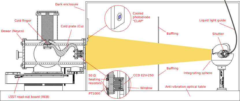
Figure 1: Laboratory setup. The QTH lamp and the monochromator sit outside of the dark enclosure and are not drawn. The light from the monochromator exit slit is conveyed through a liquid light guide (Newport 77639 Liquid Light Guide, 2 m long, 8 mm diameter) which feeds the integrating sphere. Exposure time is controlled through a mechanical shutter placed between the end of the light guide and the sphere entrance port. Our cooled photodiode (“CLAP”) is attached on the dark box wall just above the dewar window, and allows to measure the effective exposure time (see fig. 2 below).

Our test CCD is temperature-controlled at $-100\pm 0.01^{\circ}\text{C}$, is kept inside a Neyco Dewar at pressure below $7.10^{-7}$mbar, and is read out using the LSST electronic chain (see Juramy et al. (2014); O’Connor et al. (2016)), which runs at room temperature on our test stand, in a dedicated class 10000 / ISO-7 clean room. The clean room temperature is regulated ($\pm 0.2^{\circ}$C) to minimize temperature effects on the readout electronics. The video channels consist in a dual slope integration (performed by two 8-channel ASICs named ASPIC, see Juramy et al. (2014)) followed by a 18-bit ADC. In our setup, the CCD is connected to the readout electronics by two flex cables (one per half CCD, and per ASPIC), which also transport the CCD clocking lines. The sequencing of read out is delivered by an FPGA driving the CCD clocks (through appropriate power drivers) and the analog integration chain. We typically read at 550 kpix/s (so that the image is read out in 2 s) and measure a readout noise of $\sim$ 5 el per pixel. The gains are about 0.7 el/ADU. This setup achieved a gain stability of the full video chain over 3 days of a few $10^{-4}$ and always better than $10^{-4}$ within the 1-h time frame needed to measure the overall response non-linearity once, as described below.

For flat field studies, our light source is a Newport 69931 QTH (Quartz Tungsten Halogen) lamp, operated at a regulated power of 240 W, which feeds a monochromator via a lens and an order blocking filter, when needed. For the data presented below, the monochromator is set to 650 nm with a slit width of about 15 nm. The light is conveyed into the dark box via an optical fiber (Newport 77639 Liquid Light Guide, 2 m long, 8 mm diameter). A mechanical shutter is placed between the end of the fiber and the entrance port of the integrating sphere. A cooled photodiode (Cooled Large Area Photodiode, “CLAP”, see Regnault et al. (2015), appendix F) is attached to the dark box wall and placed above the dewar window; it is readout using a low-noise ASIC pre-amplifier, with $\sim$ 300 Hz bandwidth, feeding a 31.25 kHz flashing ADC. The Dewar is attached to one side of the dark box, and sees the integrating sphere at a distance of $\sim$ 1 m (see fig. 1). The illumination system delivers about 10,000 photoelectrons per second and per CCD pixel for a $\sim 15$ nm bandwidth. Our test bench is similar to the one described in O’Connor et al. (2016) for LSST CCD acceptance test.

The CCD is operated within the vendor recommendations (see table 1): the drift field is created by applying -70 V to the back substrate (namely the light entrance window of the sensor). The CCD250 is a 4-phase device, and during integration, we set 2 phases low and 2 phases high. Even for short integrations, we do not run faster than $\sim$3 images per min, which is the expected acquisition rate of LSST.

Voltage Name	Line	Voltage Value
Back Substrate bias	BS	-70.0 V
Guard Diode	GD	26. V
Output amplifier Drain	OD	30. V
Output Gate	OG	3.3 V
Reset transistor Drain	RD	18. V
Serial lines Low	SL	0.6 V
Serial lines High	SU	9.8 V
Parallel lines Low	PL	0.06 V
Parallel lines High	PU	9.3 V
Reset Gate Low	RGL	-0.02 V
Reset Gate High	RGU	11.8 V

Table 1: Voltages used to operate the e2v-250 CCD.

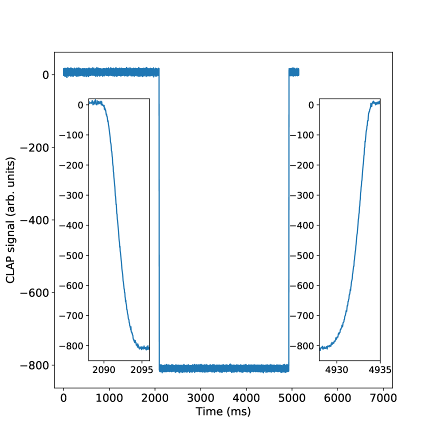
Figure 2: Waveform acquired from our photodiode for a $\sim 3\,\text{s}$ exposure. The insets display the signal edges, which result from the shutter motion rather than the bandwidth of the electronics.

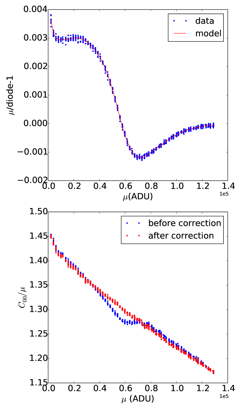
Figure 3: Top: integral non-linearity of channel 8, and the spline model (with 14 knots) we use to correct for it. Bottom: $C_{00}/\mu$ before and after non linearity correction. We see that the main distortion has disappeared.

Figure 4: Spline fits to integral non-linearity of the 16 channels. The main differences between various channels are the overall gains (the two groups correspond to the two different chips hosting the preamplifiers), and the low signal level behavior (presumably due to the on-CCD amplifier).

In order to measure the non-linearity of the electronic chains, we use the photodiode to measure the delivered light, integrating numerically the digitized waveform, an example of which is shown in figure 2. Our video channels are affected by a small non-linearity, which we measure and correct (fig. 3). In order to vary the integrated charge in the CCD image, we vary the open-shutter time at a somehow constant illumination intensity, ensured by our light source regulation. The photodiode hence delivers a current essentially independent of the exposure time, and our non-linearity measurement does not rely on its electronics being linear. We determine a non-linearity correction for each channel and apply it to the input data. We note that correcting the variances for differential non-linearity is more important than correcting the signal levels for integral non-linearity. In the image series we consider here, the pedestals do not vary by more than 10 ADU’s, and so, wondering if the non-linearity should be corrected before or after pedestal subtraction is pointless. Figure 4 displays the correction for the 16 channels, and one can notice that the distortions are mostly similar. The prominent dip at roughly half the full range resembles in size and shape the non-linearity measured when testing the pre-amplifier, namely the ASPIC circuits. One may note that although our photodiode system allow us to measure the actual open-shutter time, we do not rely on this capability when establishing the non-linearity correction. The plots in fig. 3 display the data of 10 successive acquisitions and allows one to visually judge the overall stability of the gain.

5.2 Dataset and processing

We use here 1000 pairs of flat field images (at 650 nm, as described above). We refer here to pairs, because all variance or covariance measurements are carried out on pixel to pixel subtractions of pairs of flat fields at the same intensity, in order to eliminate the contribution of illumination or response non-uniformity to the measurements. The data is acquired as 10 successive sequences of flat pairs of increasing intensity, so that a slowly varying gain (because e.g. of temperature variations) does not distort differently low- and high-intensity images.

We first subtract the pedestal from the image, measured on the serial overscan (ignoring the first 5 columns). We tried several approaches : subtracting a global value per amplifier, and subtracting from each line the median of its overscan. The latter leaves residual covariance of order of 2 el² along the serial direction, and we eventually settled for a spline smoothing of the overscan along the parallel direction. We then get residual covariances along the serial direction of about $0.2$ el².

We clip 10 pixels on the four sides of the $512\times 2002$ pixel area of each channel, because at low and high x (i.e. serial direction) and at low y (parallel direction), the response of the sensor varies rapidly because of distortions of the drift field near its edges. This clipping is not required for all channels, but it allows us to safely compare measurements from different channels.

The variances and covariances are computed from spatial averaging, and using subtractions of image pairs of the same intensity eliminates the contributions from non-uniformity of illumination or sensor sensitivity. We however have to clip bad pixels, typically cosmetic defects and ionizing particle depositions. To this end, we first clip 5 $\sigma$ outliers in each image of the pair, and then clip 4 $\sigma$ outliers on the subtraction. Toy Monte Carlo simulations show that the bias on variance is $10^{-3}$ and twice as much for covariances. We compensate this small bias in the analysis that follows. With a cut at 3 $\sigma$ on the subtraction, the bias of the variance would be about 2.7 %, and again twice as large for covariances.

One might wonder if the outlier clipping varies with signal level. We find on average that there are 8 more pixels (per channel of $10^{6}$ pixels) clipped at high flux ($10^{5}$ el) as compared with low flux. If we attribute these 8 pixels to the tails of a Gaussian distribution, the relative loss in variance is 1.4 $10^{-4}$. This corresponds to a loss of variance of about 10 el², while the effects we are discussing later are at least of the order of a few hundred. Furthermore, since the number or clipped pixels varies smoothly with signal level, most of the (small) induced bias is firstly absorbed by the gain.

We carry the computation of covariances in the Fourier domain (the code is provided in appendix A), because it is faster than in direct space as soon as one computes covariances for more than about $5\times 5$ separations, and even less if fast Fourier transforms are computed for image sizes which are powers of 2. In terms of symmetry, $C_{i,j}=C_{-i,-j}$, because these two expressions are algebraically identical, as they involve exactly the same pixel pairs. On the other hand, $C_{i,j}$ and $C_{i,-j}$ do not involve the same pixel pairs (if both $i$ and $j$ are non zero), but are expected, from parity symmetry, to be equal on average. So, we compute both covariances (for $i\neq 0$ and $j\neq 0$) for sake of statistical efficiency, and report their average. For small correlations, the statistical uncertainty of a covariance estimate is:

$$\sigma\left(\hat{C_{ij}}\right)=V/\sqrt{N}$$ (21)

for $i$ or $j$ non zero, where V is the variance of the pixel distribution, and N is the number of pixel pairs used to evaluate the covariance. The uncertainty of the variance estimation is twice as large. With $\sim$ $10^{6}$ pixels per channel and image, and 1000 image pairs, we measure each correlation ($C_{ij}/V$) with an (absolute) uncertainty of $\sim 3\leavevmode\nobreak\ 10^{-5}$, for each channel. The figure improves by a factor of 4 when averaging over the 16 channels, and by $\sqrt{2}$ when both $i$ and $j$ are non zero.

5.3 Deferred charge

Variance and covariances can be affected by contributions unrelated the brighter-fatter effect, in particular imperfect charge transport: if a small fraction of a charge belonging to a pixel is eventually read out into its neighbor, a statistical correlation between neighbors will build up. The quality of charge transport in CCDs is commonly studied using “overscans”, which correspond to clock and read out cycles beyond the physical number of rows and/or columns. Charges measured in these first overscan pixels are deferred signals, and are commonly used to measure charge transfer inefficiencies (CTI), in both the serial and parallel directions.

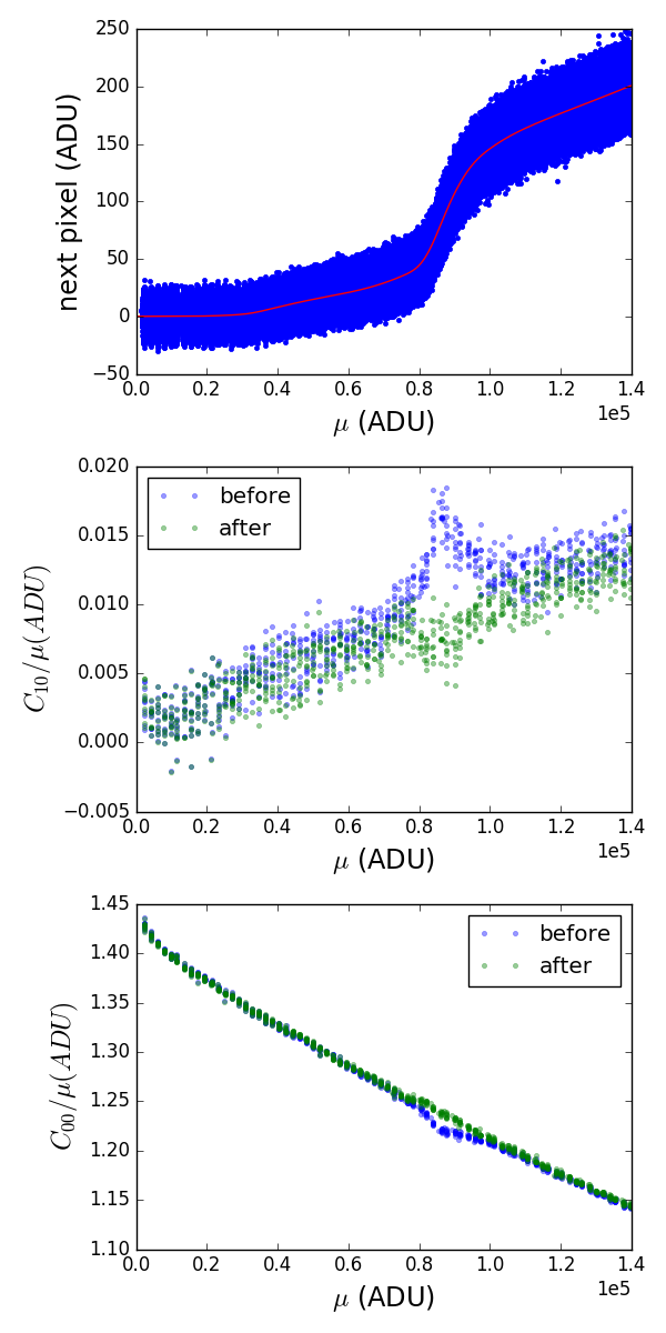
Figure 5: The 3 plots refer to channel 10 only, after linearity correction. Top: content of the first serial overscan pixel as a function of flat level (data points and a spline fit). Middle: first serial correlation as a function of flat level, before and after placing the charge back, i.e., before and after deferred charge correction. Bottom: same as middle, but for the variance. In figure 3, there is no obvious distortion of the variance curve after linearity correction because channel 8 is essentially free of deferred charge.

	$\chi^{2}_{full}/N_{dof}$	$\chi^{2}_{2}/N_{dof}$	gain	$a_{00}$	RO noise
value	1.23	4.04	0.713	-2.377 $10^{-6}$	4.54
scatter	0.10	0.27	0.020	0.032 $10^{-6}$	0.43

Table 2: Statistics of PTC fits. The $\chi^{2}$ refer to the contribution of the variance terms, although the fit actually involves variances and covariances. The scatter is evaluated over the 16 video channels. $\chi^{2}_{full}$ refers to the model of eq. 20. The scatter of the gains essentially reflects different gains of the two integrated circuits hosting the pre-amplifiers. The observed spread of $a_{00}$ across amplifiers is several times larger than expected from shot noise.

In figure 5, we display the data of channel 10 only: the top plot displays the measured content of first serial overscan pixel (after pedestal subtraction) as a function of the content of the last physical pixel, while the two bottom plots display the serial covariance, and the variance respectively. It is clear that the rapid rise in deferred charge is associated to a peak in the covariance, and a small trough in the variance. To illustrate the relation between deferred charge and covariances, let us consider two successive pixels, $p_{0}$ and $p_{1}$, each leaving some deferred charge $\epsilon$ behind. $p_{1}$ becomes:

$$p^{\prime}_{1}\equiv p_{1}+\epsilon_{0}-\epsilon_{1}$$ (22)

We have:

$$Cov(p^{\prime}_{1},p^{\prime}_{0}) =Cov(p_{1},p^{\prime}_{0})+Cov(\epsilon_{0},p^{\prime}_{0})$$ (23)

$$\simeq Cov(p_{1},p_{0})+Var(p^{\prime}_{0})dE[\epsilon_{0}]/dp_{0}$$ (24)

So, the correlation between successive pixels follows the derivative of the deferred charge. Following a similar route, we get $Var(p^{\prime}_{1})\simeq Var(p_{1})[1-2dE[\epsilon_{1}]/dp_{1}]$, which means that we expect a variance deficit at the same charge levels as the peaks in the serial correlation, that can be observed on the bottom plot of fig. 5. A toy simulation confirms that transferring a signal-dependent charge to the next (time-wise) pixel produces peaks on the $C_{10}$ vs $\mu$ curve at $\mu$ values where the deferred charge varies rapidly. In the case where a constant fraction is transferred to the next pixel (possibly negative, at some point of the video chain), this causes a constant correlation offset, so mostly a linear contribution to the covariance which does not exist in the covariance models discussed above.

We do not have a clear physical model of what causes the deferred serial charge to increase rapidly at specific signal values. This non-linearity seems to exclude trailing signals in the electronic chain. Not all channels have clear $C_{10}$ peaks (for example channel 8 displayed in figure 3 is essentially free of such effects) and different channels have peaks at different $\mu$ values. These peaks remain located at the same positions expressed in number of electrons when using an other readout board or when altering the gain at the CCD level. This indicates that their cause lies in the sensor itself. The sizes of these peaks are similar in all sub-regions of the image section corresponding to a given channel. We hence attribute those to some effect happening in the pre-scan pixels of the serial register, that all collected charges have to traverse. We finally observe that the height of these peaks varies with the parallel gate voltages, which may influence the electric field in the vicinity of the serial registers. We are currently studying a possible mitigation of these peaks by altering the parallel clock levels.

We have modeled the average deferred serial charge by fitting a spline curve to the measurements (fig. 5, top), for each channel separately, based on the content of the last physical pixels and the first overscan pixels. Using this simple modeling, we pre-process the images by placing the (average) deferred charge back into the previous pixel. Once the correction is done, the peaks in the $C_{10}$ curve vanish as well as their counterparts on the variance curve (fig. 5, middle and bottom). We do not know why this simple correction procedure slightly over-corrects the $C_{10}$ peak (fig. 5 middle). In this figure, one can notice that the correction of deferred charge reduces the slope of $C_{10}/\mu$ by roughly 10%, and inspecting the model of equation 15 shows that this slope drives the $a_{10}$ coefficient value.

We note that the correction procedure we used assumes that all columns are affected in the same way, i.e. that all charges go through the defect causing deferred charge. This is justified by covariances measured separately for different set of columns being similar, and by the “pocket-pumping” technique (see e.g. §5.3.4 in Janesick 2001) not unveiling traps in the serial register.

The parallel transport of this sensor is far better than the serial one: we typically measure a few ADUs of deferred signal close to saturation, as compared to more than 100 ADUs in the serial direction. We hence decided to not correct for this small effect. We convert the measured values of deferred charge into the commonly used CTI figure: the channel displayed in fig. 5 has a high signal serial CTI of $200/1.4\leavevmode\nobreak\ 10^{5}/522\simeq 3\leavevmode\nobreak\ 10^{-6}$, where $522$ is the number of pixels in the serial register. The highest accepted serial CTI for LSST is set to $5\leavevmode\nobreak\ 10^{-6}$. The parallel CTI of this sensor is better than $2\leavevmode\nobreak\ 10^{-8}$at high flux.

We finish this section by one more puzzling observation: the channel displayed in fig. 5 has a gain of approximately 0.7 (el/ADU), meaning that the overscan pixel reaches about 130 electron at the maximum $\mu\simeq 10^{5}$ el. At this highest value, we measure a variance of $\sim$ 60 el², of which typically 25 are expected from read noise (as measured at the other end of the curve). So, at $10^{5}$ el, the variance of the deferred charge ($\sim 35$ el²) is less that one third of its average ($\sim 130$), i.e. much less than expected from Poisson statistics. At all values, the measured deferred charge fluctuates much less than expected from Poisson fluctuations and read noise. A physical model for this deferred charge would have to accommodate this observation, but this goes beyond the scope of this paper.

6 Analysis of the Photon Transfer Curve and covariance curves

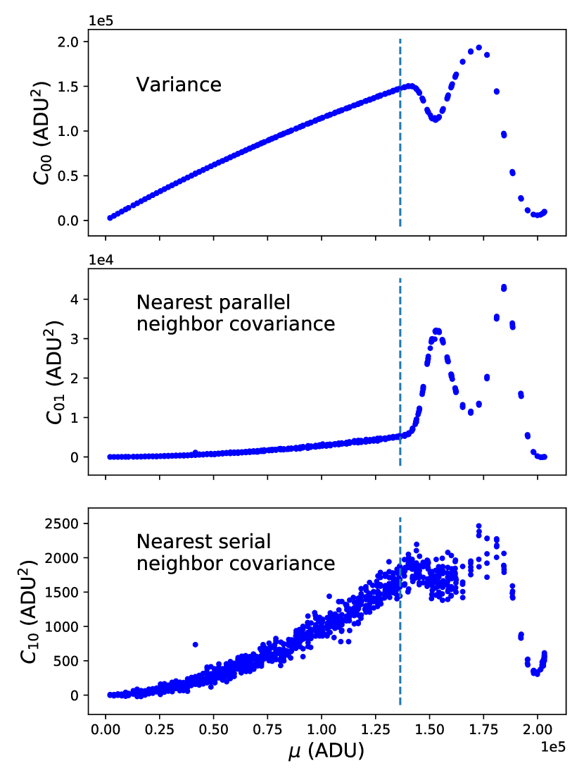
Figure 6: Variance and two nearest covariances as a function of flat field average, in order to illustrate the saturation level (in channel 0). The three curves change behavior around 1.5 $10^{5}$ ADUs. The drawn fitting limit is about 10% below this value, and corresponds to $10^{5}$ el, at a gain of 0.733.

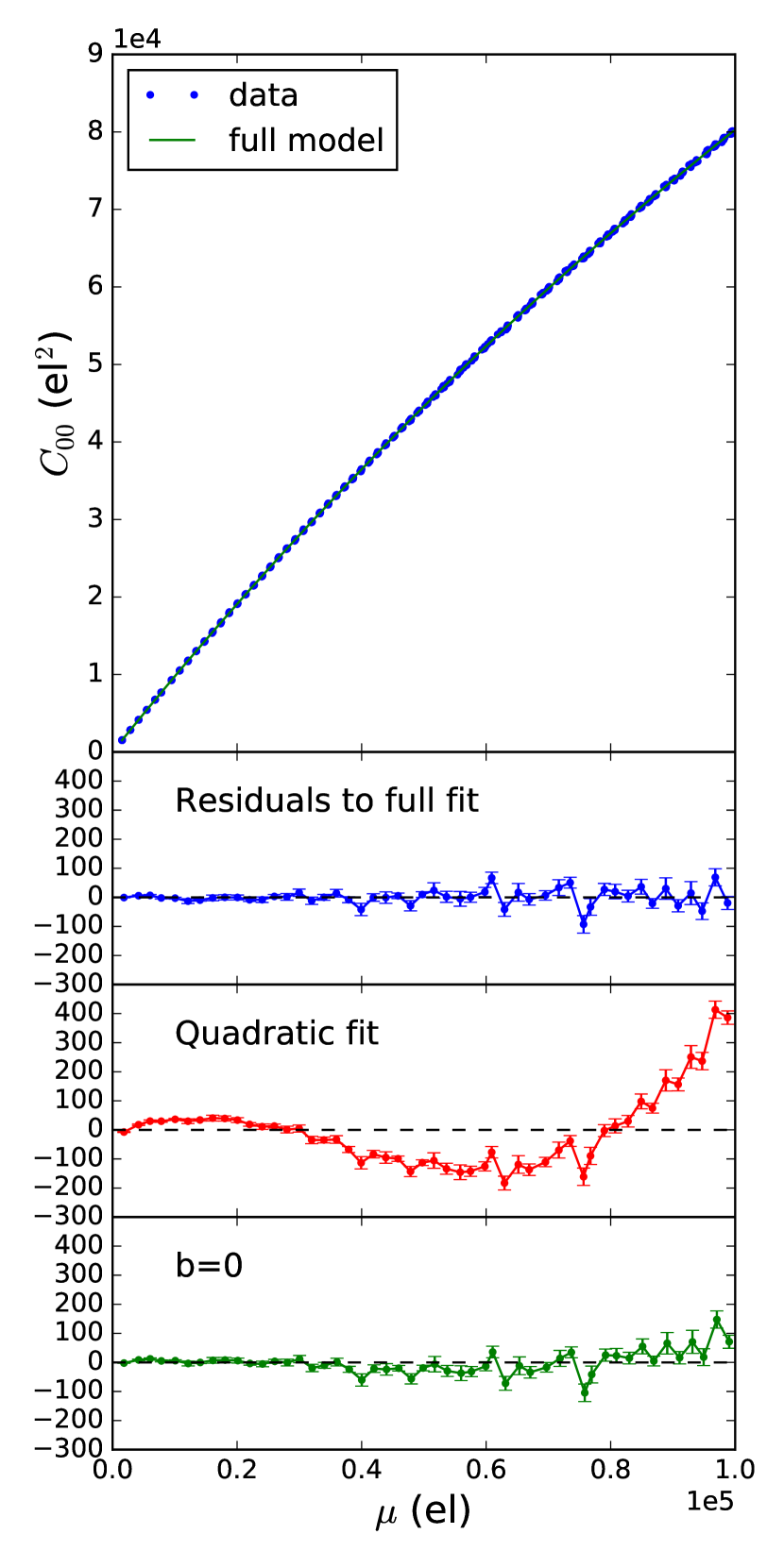
Figure 7: PTC of channel 0 fitted with three different models : the full model, a quadratic fit, and the “simple model” with $b=0$. The bottom plots display the fit residuals. The full model and the $b=0$ model describe well the data, although the $\chi^{2}$ is 10% higher for the latter. We believe that part of the fit residuals are artifacts caused by the non-linearity and deferred charge corrections.

We now confront the models presented above to our data set. We fit the $C_{ij}$ vs $\mu$ relation with two models, eq. 15 and 20, up to terms in $(\mu g)^{3}$ in the bracket. The fitted parameters are the gain, the $a_{ij}$ and $n_{ij}$ quantities, and when applicable $b_{ij}$. For $\mu$, we simply use the average between the two members of the image pair.

We fit 64 $C_{ij}$ curves with $i<8$ and $j<8$, because beyond this separation, the signal is much smaller than shot noise, for our data sample. We fit separately each readout channel, using scipy.optimize.leastsq, without binning the data. The uncertainties are derived from shot noise. We iteratively reject outliers measurements at the 5 $\sigma$ level, where the cut is derived from the scatter of the residuals. We initialize the parameters from separate polynomial fits to each separation. The fit takes a few seconds (on a core i7 CPU) for about 50,000 measurements. In the figures we display here, we generally choose to display $C_{ij}/\mu$ rather than correlations ($C_{ij}/C_{00}$), because the latter involve the measured variance, itself affected by the brighter-fatter effect.

We first have to decide up to which charge value we should fit. Variance and nearest neighbor covariances change behavior at similar filling levels, as shown on fig. 6, and it is then fairly easy to define a saturation. We arbitrarily choose a margin of about 10% below this saturation, which makes $10^{5}$ el. All fits that are described here are carried out to up to this level. Applying this cut involves some iterative procedure since it requires to know the gain, which requires some crude fit of the PTC (we use a third degree polynomial).

Figure 8: PTC of all channels (namely $C_{00}/\mu$), offset by 0.01 times the channel number. The curves going through the data points correspond to the full fit. The statistics associated to these fits are provided in table 2.

Figure 7 displays the PTC fit result of channel 0, and residuals to the two models above, and to a parabolic fit. The inadequacy of the parabolic fit is clear, but allowing for a non-zero $b$ term does not dramatically improve the fit quality at least visually, although the $\chi^{2}$ goes down by $65$ on average (over channels) for a single extra parameter. The PTCs of the 16 channels are shown in Figure 8 and Table 2 details the outcome of the data fits regarding the PTC itself (i.e. $C_{00}$). We find that the model from eq. 20 describes the data fairly well, although $\chi^{2}$ are higher than expected from shot noise, which we attribute to imperfections of the non-linearity and deferred charge corrections, which are both localized in $\mu$ because we use highly flexible functions to model both. The excess in $\chi^{2}$ corresponds to offsets at the $2\ 10^{-4}$ level r.m.s.

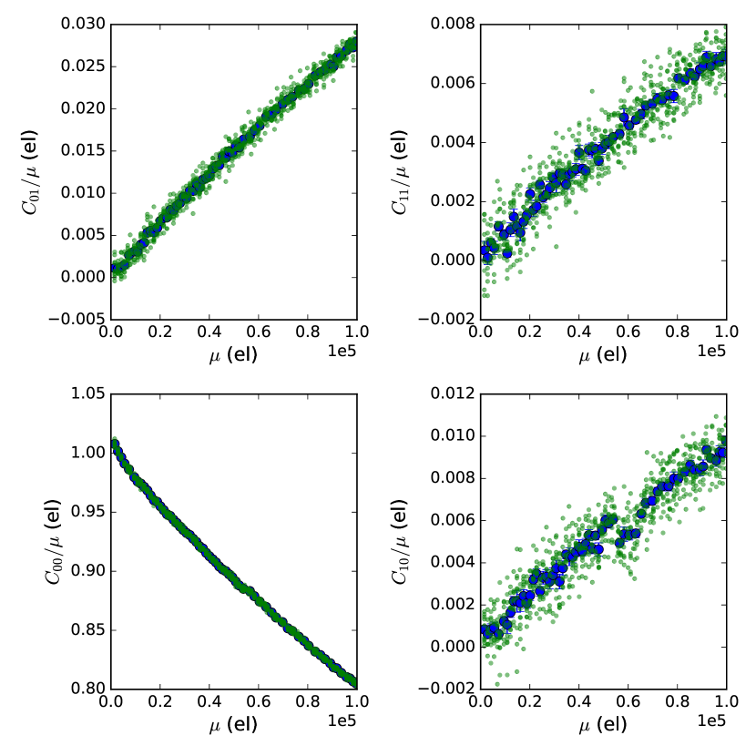
Figure 9: Nearest neighbor covariances for channel 10, and variance (divided by $\mu$). We display both the individual measurements and binned values. All quantities are expressed in electron units. The spread is similar for all plots but appears differently because scales are different. The wiggle on $C_{10}$ around $\mu=0.6\ 10^{5}$ is a remainder of the deferred charge correction (§5.3). It is clear that the data does not follow straight lines.

The next step is to study the covariance fits. We first illustrate the data by displaying the variance and 3 nearest neighbor covariances in fig. 9 for channel 10, which is affected by a varying deferred charge. All covariance measurements have similar statistical uncertainties, so the best relative uncertainties are obtained for the highest covariances, i.e. for the nearest neighbors. We first display the fit of the largest covariance i.e. $C_{01}$ (which is not affected by deferred charge). We display the fits results in fig. 10 to each channel separately and report the statistics of these fits in table 3. Visually, it is very clear that $b\neq 0$ is required. Allowing for $b\neq 0$, the $\chi^{2}$ goes down by 106 on average over channels, for a single extra degree of freedom. Taken at face value, the sense of $b_{01}$ is that the effect of a given charge on its nearest parallel neighbor pixel is 17 % larger at $\mu=10^{5}$ el  than linearly extrapolated from low-average data. The spread of this 17 % figure, as measured over the 16 channels, is only 3%.

	$a_{01}$	$b_{01}$	$\chi^{2}/N_{dof}$
value	3.32 $10^{-7}$	1.71 $10^{-6}$	1.03
scatter	0.06 $10^{-7}$	0.29 $10^{-6}$	0.04

Table 3: Statistics of $C_{01}$ curve fits (mean and r.m.s. scatter over read out channels). The scatter of $a_{01}$ over channels is about twice as large as expected from shot noise.

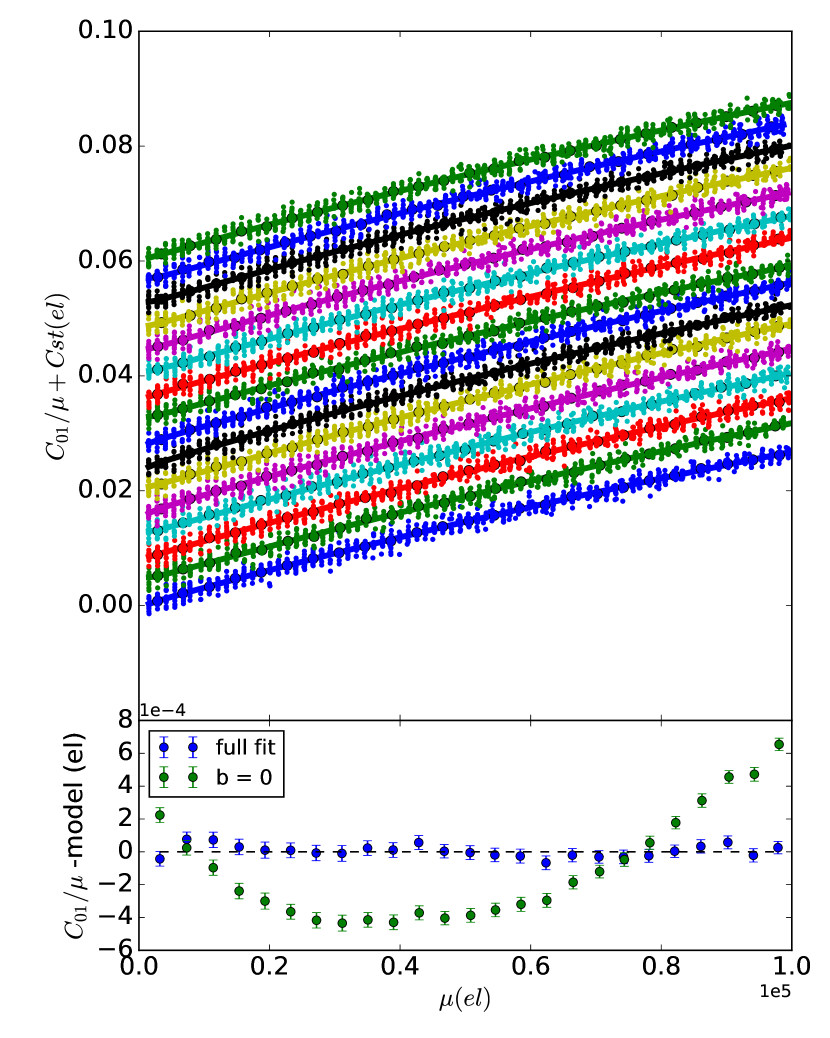
Figure 10: Fits of $C_{01}/\mu$ as a function of $\mu$ for the 16 channels. On the top plot, the data and model (the full model of eq 20) have been offset by $0.004\times c$ where $c$ is the channel number. We plot, both individual measurements and averages at the same intensity, where the error bars reflect the scatter (compatible with the expected shot noise). The bottom plot reports the binned average residuals to both fits.

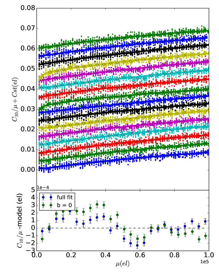
Figure 11: Fits of $C_{10}/\mu$ as a function of $\mu$ for the 16 channels. On the top plot, the data and model (the full model of eq 20) have been offset by $0.004\times c$ where $c$ is the channel number. We plot, both individual measurements, and averages at the same intensity, where the error bars reflect the scatter (compatible with the expected shot noise). The down turn at low flux of channels 8 and 12 is accommodated in the fit by the $n_{10}$ term in the model equation 20. The bottom plot reports the binned average residuals to both fits.

The nearest serial neighbor covariance $C_{10}$ is much noisier than $C_{01}$, because the covariance is about 2.5 times smaller, and wiggles have survived the deferred charge correction. We however display the fit results in figure 11 and the fit statistics table in table 4. The scatter of the measured coefficients is again larger than expected from shot noise, by about a factor of 3 for $a_{10}$, although the $\chi^{2}$ of the fits are close to the statistical expectation. The $\chi^{2}$ improvement due to $b\neq 0$ is 17 on average over channels. Note that $b_{10}$ is negative, i.e., the anisotropy of nearest neighbor covariances seems to increase with charge levels.

	$a_{10}$	$b_{10}$	$\chi^{2}/N_{dof}$
value	1.26 $10^{-7}$	-1.77 $10^{-6}$	1.03
scatter	0.08 $10^{-7}$	0.97 $10^{-6}$	0.07

Table 4: Statistics of $C_{10}$ curve fits (mean and r.m.s. scatter over read out channels). The scatter of $a_{10}$ over channels is about three times larger than expected from shot noise.

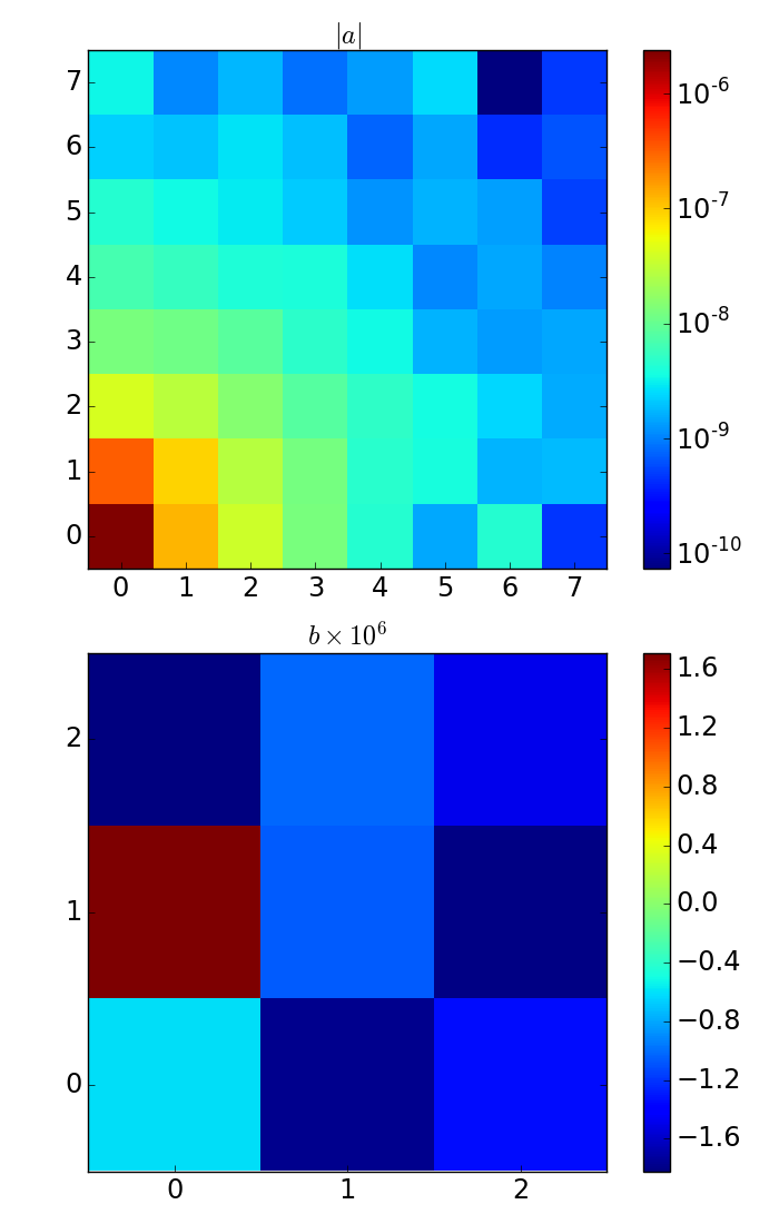
Figure 12: Color display of $a$ and $b$ arrays fits, averaged over channels. The parallel direction is vertical.

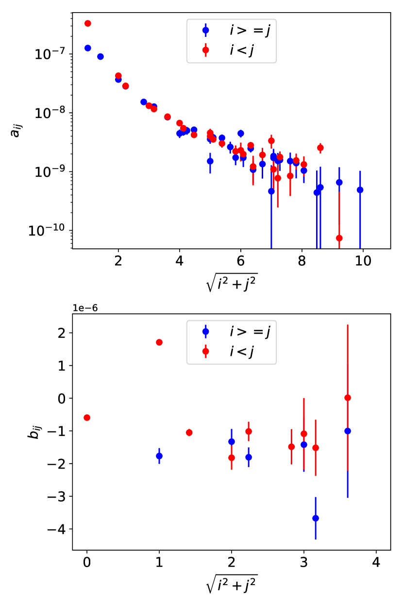
Figure 13: Values of $a$ and $b$ arrays fits, averaged over channels, as a function of distance. Error bars represent the uncertainty of the average, derived from the observed scatter. One can notice that $b$ values are mostly negative.

Figure 12 displays the fitted $a$ and $b$ values, averaged over channels. At increasing distances, $a$ decays rapidly and becomes isotropic, as visible in fig 13 (top). In figure 13, we display the $a$ and $b$ values averaged over channels, as a function of distance, with error bars representing the uncertainty on the average, derived from the observed scatter. One can deduce that, with our data, individual $a$ values are measured down to distances of about 8 pixels, and $b$ values down to about 3 to 4 pixels. For a fit to some electrostatic model, one could use even farther measurements with proper weights. As already noted $b_{01}$ and $b_{10}$ are found of opposite signs, and examining the bottom plot of fig. 13, one observes that $b$ values are mostly negative, with the notable exception of $b_{01}$. A positive $b_{01}$ can be due to the cloud getting broader in the parallel direction as charge accumulates. We can then imagine two distance-independent contributions to $b$: first the decay of the drift field due to stored charges (sometimes referred to as space charge effect), or the electron clouds center of gravity gradually changing distance to the parallel clock stripes as charge accumulates. The first effect would cause positive $b$ values, and hence, if present, has to be sub-dominant. If one attributes the negative $b$ to the second effect, the wells have to move closer to the clock stripes as charge accumulates. Regarding the stored charge diminishing the drift field (or space charge effect), one should note that even if this effect contributes to flat field electrostatics, it is in practice mostly absent from science images which usually have low to moderate sky background levels.

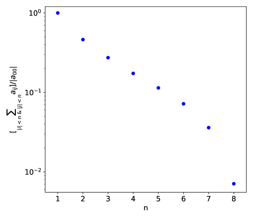
Figure 14: Cumulative sum of $a_{ij}$ as a function of maximum separation. This plot displays the average over channels.

One final analysis point is the empirical verification of the sum rule in eq. 2, that we have not enforced in the fit. On average over channels, we find:

$$\sum_{-8<k,l<8}a_{kl}=-1.6\ 10^{-8}\pm 5.7\ 10^{-8}$$ (25)

where the uncertainty reflect the scatter (to be divided by 4 for the uncertainty of the average). To set the scale, $a_{00}\simeq-2.4\ 10^{-6}$, i.e. the sum rule is satisfied down to the % level, thus indicating that the effects we measure are mostly due to charge redistribution. Figure 14 displays the sum as a function of maximum separation, and shows that, for our sensor, about 1% of the area lost (or gained) by a pixel due to its charge content is transferred to pixels located 7 or more pixels away.

We finish this paragraph by a short technical note about the fitting approach: we have considered fitting in Fourier space rather than in direct space because the expression of the model does not involve convolutions. This is however the only benefit over direct space: first, starting from covariances in direct space, one has to Fourier transform those, and the mandatory zero padding correlates the transformed data (which would otherwise be statistically independent because measured covariances have uncertainties independent of the separation). Second, one can think that different “reciprocal separations” in Fourier space could be fitted independently, but the common gain parameter still imposes to fit all the data at once. Finally, it is trivial to concentrate on small distances in direct space, but selecting large-k modes in the power spectrum of image pairs requires manipulating a lot of data. So, we have not been able to devise a simpler framework in Fourier space.

6.1 Inaccuracies of simpler analyses of covariance curves

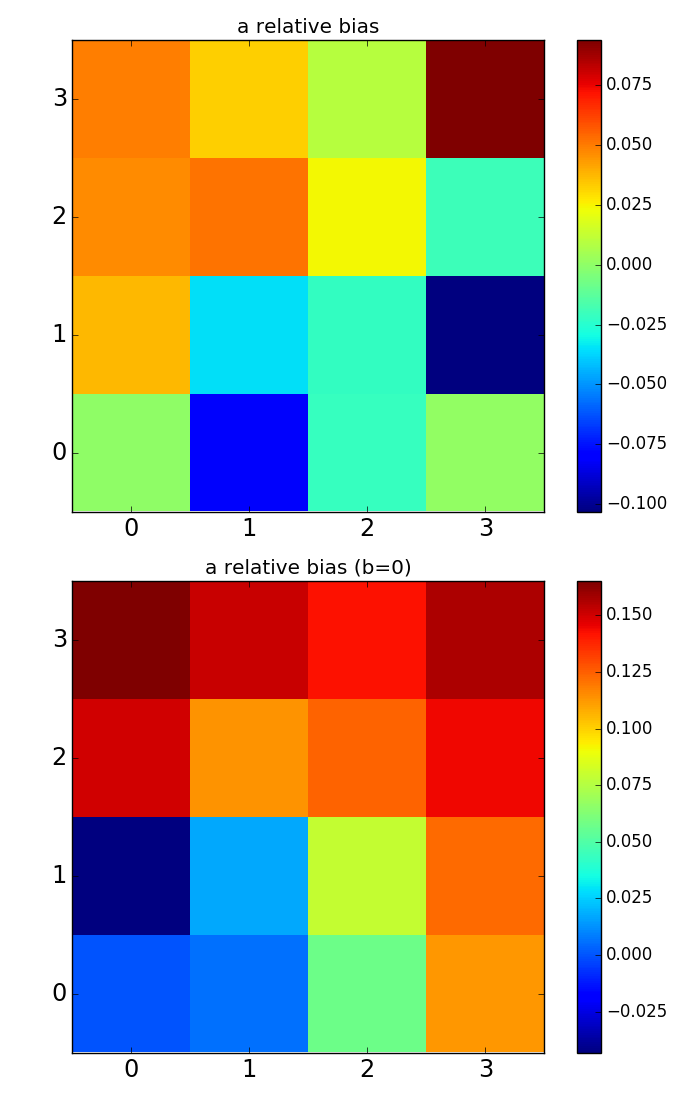
Figure 15: Relative systematic bias of the commonly used method that estimates $a_{ij}$ from the slopes of correlations, using a single illumination value at 75 ke. The top figure is for the full model, and the bottom one is for $b=0$. In the top case the nearest neighbors $a_{ij}$ are biased by +8% and -4% respectively. For the bottom case, there is a global overestimation of the effect, increasing with distance.

Many works in the literature using pixel covariances to constrain (and correct) the brighter-fatter effect (Antilogus et al. 2014; Guyonnet et al. 2015; Gruen et al. 2015; Coulton et al. 2018) assume that pixel correlations are linear with respect to illumination level, i.e. :

$$C_{ij}=a_{ij}V\mu$$ (26)

where $V$ generally represents the measured variance $C_{00}(\mu)$, and sometimes only one intensity (preferably high, in order to optimize the S/N) is being measured. Using the expression above is a simplification, as compared to equations 15 and 20. We evaluate the biases caused by this simplification alone, using the model fits reported in the previous section. To this end, we compare $a_{ij}$ as extracted from the simplified equation above with the one of the model used to evaluate $C_{ij}$ and $C_{00}$. As in the previous section, we study both the full fit result and the $b=0$ case. In figure 15, we display the relative difference between $a_{ij}$ evaluated using the above equation and the model value, for a measurement that would be performed at 75 ke (a value representative of the data studied in Guyonnet et al. 2015), averaging over the 16 video channels. We see that for the full fit ($b\neq 0$), the nearest neighbor coefficients are offset by -8% and +4% respectively. Using these biased inputs to correct science images not only compromises the measurement of the size of the PSF, but more importantly causes spurious PSF anisotropy. For the case where $b=0$, we see that essentially all $a_{ij}$ are overestimated (except $a_{01}$, biased by -4%), with a relative bias increasing with separation, up to more than 10 % at distances of $\sim 3$. For both models, the bias arises from neglecting (or approximating) terms beyond $\mu^{2}$ in equations 15 and 20. Depending on the considered sensor, it is plausible that the limitations of the brighter-fatter effect corrections observed empirically (e.g. Guyonnet et al. 2015; Mandelbaum et al. 2018) are partly due to the oversimplification implied by eq. 26.

6.2 Non-electrostatic contributions to covariances

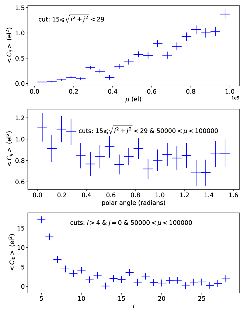
Figure 16: These figures display distant covariances, averaged over the 16 channels. Top: average value of distant covariances as a function of flat field average. Middle: the average of covariances as a function of angle shows no excess in the serial direction (angle = 0). Bottom: covariances along the serial direction, which do not exhibit any obvious structure on top of the decay expected from electrostatics.

In order to identify non-electrostatic contributions to covariances, we consider covariances at large distances, where electrostatic contributions are expected to be negligible. From a simple electrostatic model tuned on the well-measured nearest neighbors correlations, one can readily infer that electrostatically-induced covariances beyond a separation of $\sim 12$ are expected to be much lower than 1 el² at a flat field average of 50 ke, and not detectable with our statistics. Reproducing the shape of the long distance decay of electrostatic covariances is not involved because the source of the disturbing field (i.e. the charge cloud within a pixel potential well) can then be considered as a point source without a significant loss of accuracy.

Figure 16 shows that long-distance covariances are larger than expected from electrostatics only and they are increasing with the flat field average. We do not know the cause of this small distant signal, which seems almost isotropic. It is however smaller than covariances up to separations of about 8, and so does not deserve a correction for the analysis we did in the previous section. The bottom plot of figure 16 shows the serial correlation decaying as expected, but at some point, it displayed an oscillating pattern associated to a gain oscillation at 40 kHz induced by a pickup affecting the clocking of the FPGA and in turn the duration of the analog integration windows for signal and pedestal. This was solved by damping the injection by the switching power supply sourcing the noise, and using a phase-locked loop on the FPGA clocks.

7 Discussion

We have developed a framework to analyse photon transfer curves and covariance curves, starting from some model of the effect of stored charges on incoming currents. This framework allows one to constrain the electrostatic distortions as a function of separation and charge level, using large-statistics flat field data, covering a large dynamical range. In order to exploit our high-statistics data set, we had to correct for the read out chain non linearity and deferred charge effects. In a separate study, we are investigating if altering the operational voltages of the sensor reduces deferred charge effects.

Our model shows that approximating the charge-induced pixel area changes by the slope of correlation curves can lead to sizable errors, depending on the sensor, but typically scaling as $a_{00}\mu$, and which in turn bias the $a_{ij}$ measurements by a few %. Our analysis of flat field data shows that, for the e2v sensor we are studying (and under the chosen operational conditions), assuming that pixel boundaries shift linearly with source charges should be questioned. We have not yet explored the practical consequences of this finding when it comes to modeling the brighter-fatter effect on science images. One should remark that the image contrasts in uniform images are small as compared to the ones in science images, by typically two orders of magnitude or more. One should question if the low-constrast measurements carried out in flat fields apply directly to higher constrast images (see e.g. Rasmussen et al. (2016)). We are then attempting to devise practical tests of this apparent non-linearity using high contrast images.

Finally, we note that all attempts to correct the brighter-fatter effect following the framework proposed in Guyonnet et al. (2015) typically leave of the order of 10 % of the initial effect in the images (Guyonnet et al. 2015; Gruen et al. 2015; Mandelbaum et al. 2018). We have identified in this work a set of effects that could contribute to these residual PSF variation with flux by biasing the measurements of electrostatic forces at play: non-linearity of the electronic chain, covariances induced by non-electrostatic sources, oversimplification of the flux dependence of variance and covariances, small biases in variance and covariance estimates. These small contributions can conspire to leave a flux-dependent PSF after correction of the images for the brighter-fatter effect.

Appendix A Computation of covariances in the Fourier domain

We provide here a sample of the Python code we use to compute covariances in the Fourier domain, together with the calculation in direct space used to check that results are identical, and to compare the computing speeds. In order to avoid that pixels at the end of (e.g.) a line are correlated with the ones at the beginning, one has to zero-pad the data provided as input to the discrete Fourier transform (DFT), in both directions, with at least as many zeros as the maximum considered separation. With numpy.fft, zero-padding is done internally by providing the wanted size (called shape in Python parlance) of the DFT. One technical note is required here: when using DFT for real images (numpy.fft.rfft2), one should provide an even second dimension for the direct transform in order for the inverse transform (irfft2) to return the original data (up to rounding errors).

Here are the Fourier and direct routines :

import numpy as np

def compute_cov(diff, w, fft_shape, maxrange) :
    """
    diff : image to compute the covariance of
    w : weights (0 or 1) of the pixels of diff
    fft_shape : the actual shape of the DFTs
    maxrange: last index of the covariance to be computed
    returns cov[maxrange, maxrange], npix[maxrange,maxrange]
    """
    assert(fft_shape[0]>diff.shape[0]+maxrange)
    assert(fft_shape[1]>diff.shape[1]+maxrange)
    # for some reason related to numpy.fft.rfftn,
    # the second dimension should be even, so
    my_fft_shape = fft_shape
    if fft_shape[1] %2 == 1 :
        my_fft_shape = (fft_shape[0], fft_shape[1]+1)
    # FFT of the image
    tim = np.fft.rfft2(diff*w, my_fft_shape)
    # FFT of the mask
    tmask = np.fft.rfft2(w, my_fft_shape)
    # three inverse transforms:
    pcov = np.fft.irfft2(tim*tim.conjugate())
    pmean= np.fft.irfft2(tim*tmask.conjugate())
    pcount= np.fft.irfft2(tmask*tmask.conjugate())
    # now evaluate covariances and numbers of "active" pixels
    cov = np.ndarray((maxrange,maxrange))
    npix = np.zeros_like(cov)
    for dx in range(maxrange) :
        for dy in range(maxrange) :
            # compensate rounding errors
            npix1 = int(round(pcount[dy,dx]))
            cov1 = pcov[dy,dx]/npix1-pmean[dy,dx]*pmean[-dy,-dx]/(npix1*npix1)
            if (dx == 0 or dy == 0):
                cov[dy,dx] = cov1
                npix[dy,dx] = npix1
                continue
            npix2 = int(round(pcount[-dy,dx]))
            cov2 = pcov[-dy,dx]/npix2-pmean[-dy,dx]*pmean[dy,-dx]/(npix2*npix2)
            cov[dy,dx] = 0.5*(cov1+cov2)
            npix[dy,dx] = npix1+npix2
    return cov,npix

def cov_direct_value(diff ,w, dx,dy):
    (ncols,nrows) = diff.shape
    if dy>=0 :
        im1 = diff[dy:, dx:]
        w1 = w[dy:, dx:]
        im2 = diff[:ncols-dy, :nrows-dx]
        w2=w[:ncols-dy, :nrows-dx]
    else:
        im1 = diff[:ncols+dy, dx:]
        w1 = w[:ncols+dy, dx:]
        im2 = diff[-dy:, :nrows-dx]
        w2 = w[-dy:, :nrows-dx]
    w_all = w1*w2
    npix = w_all.sum()
    im1_times_w = im1*w_all
    s1 = im1_times_w.sum()/npix
    s2 = (im2*w_all).sum()/npix
    p = (im1_times_w*im2).sum()/npix
    cov = p-s1*s2
    return cov,npix