Abstract

This paper proposes a geometric estimator of dependency between a pair of multivariate samples. The proposed estimator of dependency is based on a randomly permuted geometric graph (the minimal spanning tree) over the two multivariate samples. This estimator converges to a quantity that we call the geometric mutual information (GMI), which is equivalent to the Henze-Penrose divergence Henze and Penrose (1999) between the joint distribution of the multivariate samples and the product of the marginals. The GMI has many of the same properties as standard MI but can be estimated from empirical data without density estimation; making it scalable to large datasets. The proposed empirical estimator of GMI is simple to implement, involving the construction of a MST spanning over both the original data and a randomly permuted version of this data. We establish asymptotic convergence of the estimator and convergence rates of the bias and variance for smooth multivariate density functions belonging to a Hölder class. We demonstrate the advantages of our proposed geometric dependency estimator in a series of experiments.

keywords:
Henze-Penrose mutual information, Friedman-Rafsky test statistic, geometric mutual information, convergence rates, bias and variance tradeoff, optimization, minimal spanning trees.
\pubvolume

xx \issuenum1 \articlenumber5 \TitleGeometric Estimation of Multivariate Dependency \AuthorSalimeh Yasaei Sekeh and Alfred O. Hero \AuthorNamesSalimeh Yasaei Sekeh and Alfred O. Hero

1 Introduction

Estimation of multivariate dependency has many applications in fields such as information theory, clustering, structure learning, data processing, feature selection, time series prediction and reinforcement learning, see Lewi et al. (2006) and Peng et al. (2002), Moon et al. (2017), Brillinger (2004), Torkkola (2003); Vergara and A. (2014); Peng et al. (2005, 1997), Sorjamaa et al. (2005), and Mohamed and Rezende (2015), respectively. It is difficult to accurately estimate the mutual information in high dimensional settings where the data is multivariate with a Lebesgue continuous density—the setting considered in this paper. An important and ubiquitous measure of dependency is the Shannon Mutual Information (MI), which has seen extensive use across many application domains. However, the estimation of mutual information can often be challenging. In this paper we focus on a measure of MI that we call the Geometric MI (GMI). This MI measure is defined as the asymptotic large sample limit of a randomized minimal spanning tree (MST) statistic spanning the multivariate sample realizations. The GMI is related to a divergence measure called the Henze-Penrose divergence Neemuchwala and Hero (2005), Neemuchwala et al. (2006), and related to the multivariate runs test Henze and Penrose (1999). In Berisha and Hero (2015), Berisha et al. (2016), it was shown that this divergence measure can be used to specify a tighter bound for the Bayes error rate for testing if a random sample comes from one of two distributions as compared to previous divergence-type bounds such as the Bhattacharrya bound. Furthermore, the authors of Yasaei Sekeh et al. (2018) proposed a nonparametric bound on multi-class classification Bayes error rate using a global MST graph.

Let 𝐗𝐗\mathbf{X} and 𝐘𝐘\mathbf{Y} be random variables with unknown joint density fXYsubscript𝑓𝑋𝑌f_{{X}{Y}} and marginal densities fXsubscript𝑓𝑋f_{{X}} and fYsubscript𝑓𝑌f_{{Y}}, respectively, and consider two hypotheses: H0subscript𝐻0H_{0}, 𝐗𝐗\mathbf{X} and 𝐘𝐘\mathbf{Y} are independent and H1subscript𝐻1H_{1}, 𝐗𝐗\mathbf{X} and 𝐘𝐘\mathbf{Y} are dependent,

H0:fXY=fXfY,versusH1:fXYfXfY.:subscript𝐻0subscript𝑓𝑋𝑌subscript𝑓𝑋subscript𝑓𝑌versussubscript𝐻1:subscript𝑓𝑋𝑌subscript𝑓𝑋subscript𝑓𝑌H_{0}:f_{{X}{Y}}=f_{{X}}f_{{Y}},\;\;\;\;\;\hbox{versus}\;\;\;\;\;H_{1}:f_{{X}{Y}}\neq f_{{X}}f_{{Y}}.

The GMI is defined as the Henze-Penrose divergence between fXYsubscript𝑓𝑋𝑌f_{XY} and fXfYsubscript𝑓𝑋subscript𝑓𝑌f_{X}f_{Y} which can be used as a dependency measure. In this paper we prove that for large sample size the randomized minimal spanning tree (MST) statistic spanning the original multivariate sample realizations and randomly shuffled data set in which for given the first element in each pair the second element is replaced by a randomly selected from all second elements, convergences to the GMI measure. A direct implication of Berisha and Hero (2015), Berisha et al. (2016) is that the GMI provides a tighter bound on the Bayes misclassification rate for the independence test of H0subscript𝐻0H_{0} vs H1subscript𝐻1H_{1}. In this paper we propose an estimator based on a random permutation modification of the Friedman-Rafsky multivariate test statistic and show that under certain conditions the GMI estimator achieves the parametric mean square error (MSE) rate when the joint and marginal densities are bounded and smooth. Importantly our proposed GMI estimator does not require explicit estimation of the joint and marginal densities.

In addition to achieving the optimal theoretical MSE rate, computational complexity is an important challenge addressed by researchers in machine learning and data science. Most plug-in based estimators like kernel density estimator (KDE) or K-nearest neighbour (KNN) estimator require runtime complexity of O(n2)𝑂superscript𝑛2O(n^{2}) which is not suitable for large scale applications. Noshad et al. proposed a graph theoretic direct estimation method based on nearest neighbor ratios (NNR) Noshad et al. (2017). The NNR estimator is based on k𝑘k-NN graph and computationally more tractable than other competing estimators with complexity O(knlogn)𝑂𝑘𝑛𝑛O(kn\log n). The construction of the minimal spanning tree lies at the heart of the GMI estimator proposed in this paper. Since the GMI estimator is based on the Euclidean MST the dual-tree algorithm by March et al. March et al. (2010) can be applied. This algorithm is based on the construction of Borůvka Borůvka (1926) and implements the Euclidean MST in approximately O(nlogn)𝑂𝑛𝑙𝑜𝑔𝑛O(nlogn) time which is faster than the previous estimators. In this paper we experimentally show that for large number of sample sizes the proposed GMI estimator is less computationally complex than the KDE plug-in method.

1.1 Related work

Estimation of mutual information is related to estimation of the information histogram. The most common estimators of MI are based on plug-in density estimation, e.g., using kernel density or kNN density estimators Kraskov et al. (2004), Moon et al. (2017). Motivated by ensemble methods applied to divergence estimation Moon and Hero (2014)-Moon et al. (2016), in Moon et al. (2017) an ensemble method for combining multiple KDE bandwidths was proposed for estimating MI. Under certain smoothness conditions this ensemble MI estimator was shown to achieve parametric convergence rates.

Another class of estimators of multivariate dependency bypasses the difficult density estimation task. This class includes the statistically consistent estimator of Rényi-α𝛼\alpha and KL mutual information which is based on the asymptotic of the length of the KNN graph, Leonenko et al. (2008) and Gao et al. (2015). The estimator of Pál et al. (2010) builds on the KNN methods for Rényi entropy estimation. As MI increases, the dependencies between random variables increase which results in less smooth densities. In Gao et al. (2015), it has been shown that for large MI the KNN or KDE approaches are ill-suited candidates for estimating MI since the assumption of local uniformity can be violated when they are strong dependencies. To overcome this issue an assumption on the smoothness of the density is required, see Krishnamurthy et al. (2014), Kandasamy et al. (2015), and Moon and Hero (2014)-Moon et al. (2016). For all of these methods, the optimal parametric rate of MSE convergence is achieved when the densities are either d𝑑d, (d+1)/2𝑑12(d+1)/2 or d/2𝑑2d/2 times differentiable Singh and Póczos (2016). In this paper, we assume that joint and marginal densities are smooth in the sense that they belong to a strong Hölder continuous classes of densities Σds(η,K)subscriptsuperscriptΣ𝑠𝑑𝜂𝐾\Sigma^{s}_{d}(\eta,K), such that the smoothness parameter η𝜂\eta ranges in (0,1]01(0,1].

A MI measure based on the Pearson divergence was considered in Sugiyama (2012) that is computational efficient and numerically stable. The authors of Costa and Hero (2004) and Pál et al. (2010) used minimal spanning tree generalized nearest-neighbor graph approaches, respectively, to estimate Rényi mutual information. In Moon et al. (2017), a nonparametric mutual information estimator was proposed using a weighted ensemble method with O(1/n)𝑂1𝑛O(1/n) parametric convergence rate. This estimator was based on plug-in density estimation, which is challenging in high dimension.

Our proposed estimator differs from previous methods in the following ways. First, it estimates a different measure of mutual information, the GMI. Second, instead of using the KNN graph the estimator of GMI uses a randomized minimal spanning tree that spans the multivariate realizations. The proposed GMI estimator is motivated by the multivariate runs test of Friedman and Rafsky (FR) Friedman and Rafsky (1979) which is a multivariate generalization of the univariate Smirnov maximum deviation test Smirnov (1939) and the Wald-Wolfowitz Wald and Wolfowitz (1940) runs test in one dimension. We also emphasize that our proposed GMI estimator does not require boundary correction, in contrast to other graph-based estimators, such as, the NNR estimator Noshad et al. (2017), scalable MI estimator Noshad and Hero (2018), or cross match statistic Yasaei Sekeh et al. (2018).

1.2 Contribution

The contribution of this paper has three components

  • (1)

    We propose a novel non-parametric multivariate dependency measure, referred to as Geometric Mutual Information (GMI), that is based on graph-based divergence estimation. The geometric mutual information is constructed using a minimal spanning tree and is a function of Friedman-Rafsky multivariate test statistic.

  • (2)

    We establish properties of the proposed dependency measure analogous to those of standard mutual information, such as, convexity, concavity, chain rule, and the data processing inequality.

  • (3)

    We derive a bound on the MSE rate for the proposed geometric estimator. An advantage of the estimator is that it achieves the optimal MSE rate without explicitly performing boundary correction, which is required for most plug-in estimators.

1.3 Organization

The paper is organized as follows. In Section 2, we define the geometric mutual information and establish some of its mathematical properties. In Subsection 2.2 and 2.3, we introduce a statistically consistent GMI estimator and derive a bound on its mean square error convergence rate. In Section 3 we verify the theory through experiments.

Throughout the paper, we denote statistical expectation by 𝔼𝔼{\mathbb{E}}, the variance by abbreviation VarVar{\rm Var}. Bold face type indicates random vectors. All densities are assumed to be Lebesgue continuous with no atoms.

2 The geometric mutual information (GMI)

In this section, we first review the definition of Henze-Penrose (HP) divergence measure defined by Berisha and Hero in Berisha and Hero (2015) and Henze and Penrose (1999). The Henze-Penrose divergence between densities f𝑓f and g𝑔g with domain dsuperscript𝑑{\mathbb{R}}^{d} for parameter p(0,1)𝑝01p\in(0,1) is defined as follows (see Henze and Penrose (1999), Berisha and Hero (2015), and Berisha et al. (2016)):

Dp(f,g)=14pq[(pf(𝐱)qg(𝐱))2pf(𝐱)+qg(𝐱)d𝐱(pq)2],subscript𝐷𝑝𝑓𝑔14𝑝𝑞delimited-[]superscript𝑝𝑓𝐱𝑞𝑔𝐱2𝑝𝑓𝐱𝑞𝑔𝐱differential-d𝐱superscript𝑝𝑞2D_{p}(f,g)=\displaystyle\frac{1}{4pq}\left[\int\frac{\big{(}pf(\mathbf{x})-qg(\mathbf{x})\big{)}^{2}}{pf(\mathbf{x})+qg(\mathbf{x})}\;{\rm d}\mathbf{x}-(p-q)^{2}\right], (1)

where q=1p𝑞1𝑝q=1-p. This functional is an f𝑓f-divergence Csiszár (1967), also known as an Ali-Silvey distance Ali and Silvey (1996). That is, it satisfies the properties of non-negativity, monotonicity, and joint convexity Berisha et al. (2016). This measure takes values in [0,1]01[0,1] and Dp=0subscript𝐷𝑝0D_{p}=0 if and only if f=g𝑓𝑔f=g almost surely.

The geometric mutual information measure is defined as follows. Let fXsubscript𝑓𝑋f_{X}, fYsubscript𝑓𝑌f_{Y}, and fXYsubscript𝑓𝑋𝑌f_{XY} be the marginal and joint distributions, respectively, of random vectors 𝐗dx𝐗superscriptsubscript𝑑𝑥\mathbf{X}\in{\mathbb{R}}^{d_{x}}, 𝐘dy𝐘superscriptsubscript𝑑𝑦\mathbf{Y}\in{\mathbb{R}}^{d_{y}} where dxsubscript𝑑𝑥d_{x} and dysubscript𝑑𝑦d_{y} are positive integers. Then by using (1), a Henze-Penrose generalization of the mutual information between 𝐗𝐗\mathbf{X} and 𝐘𝐘\mathbf{Y}, is defined by

Ip(𝐗;𝐘)=Dp(fXY,fXfY)=14pq[(pfXY(𝐱,𝐲)qfX(𝐲)fY(𝐲))2pfXY(𝐱,𝐲)+qfX(𝐱)fY(𝐲)d𝐱d𝐲(pq)2].subscript𝐼𝑝𝐗𝐘subscript𝐷𝑝subscript𝑓𝑋𝑌subscript𝑓𝑋subscript𝑓𝑌missing-subexpressionabsent14𝑝𝑞delimited-[]double-integralsuperscript𝑝subscript𝑓𝑋𝑌𝐱𝐲𝑞subscript𝑓𝑋𝐲subscript𝑓𝑌𝐲2𝑝subscript𝑓𝑋𝑌𝐱𝐲𝑞subscript𝑓𝑋𝐱subscript𝑓𝑌𝐲differential-d𝐱differential-d𝐲superscript𝑝𝑞2\begin{array}[]{l}I_{p}(\mathbf{X};\mathbf{Y})=D_{p}(f_{XY},f_{X}f_{Y})\\ \\ \qquad\qquad=\displaystyle\frac{1}{4pq}\left[\iint\frac{\big{(}pf_{XY}(\mathbf{x},\mathbf{y})-qf_{X}(\mathbf{y})f_{Y}(\mathbf{y})\big{)}^{2}}{pf_{XY}(\mathbf{x},\mathbf{y})+qf_{X}(\mathbf{x})f_{Y}(\mathbf{y})}\;{\rm d}\mathbf{x}\;{\rm d}\mathbf{y}-(p-q)^{2}\right].\end{array} (2)

We will show below that Ip(𝐗;𝐘)subscript𝐼𝑝𝐗𝐘I_{p}(\mathbf{X};\mathbf{Y}) has a geometric interpretation in terms of the large sample limit of a minimal spanning tree spanning n𝑛n sample realizations of 𝐗𝐘𝐗𝐘\mathbf{X}\cup\mathbf{Y}. Thus we call Ip(𝐗;𝐘)subscript𝐼𝑝𝐗𝐘I_{p}(\mathbf{X};\mathbf{Y}) the geometric mutual information (GMI) between 𝐗𝐗\mathbf{X} and 𝐘𝐘\mathbf{Y}. The GMI satisfies similar properties to other definitions of mutual information, such as Shannon and Rényi mutual information. Recalling (3) in Berisha and Hero (2015), an alternative form of Ipsubscript𝐼𝑝I_{p} is given by

Ip(𝐗;𝐘)=1Ap(𝐗;𝐘)=up(𝐗;𝐘)4pq(pq)24pq,subscript𝐼𝑝𝐗𝐘1subscript𝐴𝑝𝐗𝐘subscript𝑢𝑝𝐗𝐘4𝑝𝑞superscript𝑝𝑞24𝑝𝑞\displaystyle I_{p}(\mathbf{X};\mathbf{Y})=1-A_{p}(\mathbf{X};\mathbf{Y})=\displaystyle\frac{u_{p}(\mathbf{X};\mathbf{Y})}{4pq}-\displaystyle\frac{(p-q)^{2}}{4pq}, (3)

where

Ap(𝐗;𝐘)=fXY(𝐱,𝐲)fX(𝐱)fY(𝐲)pfXY(𝐱,𝐲)+qfX(𝐱)fY(𝐲)d𝐱d𝐲=𝔼XY[(pfXY(𝐗,𝐘)fX(𝐗)fY(𝐘)+q)1],andup(𝐗;𝐘)=14pqAp(𝐗;𝐘).formulae-sequencesubscript𝐴𝑝𝐗𝐘double-integralsubscript𝑓𝑋𝑌𝐱𝐲subscript𝑓𝑋𝐱subscript𝑓𝑌𝐲𝑝subscript𝑓𝑋𝑌𝐱𝐲𝑞subscript𝑓𝑋𝐱subscript𝑓𝑌𝐲differential-d𝐱differential-d𝐲subscript𝔼𝑋𝑌delimited-[]superscript𝑝subscript𝑓𝑋𝑌𝐗𝐘subscript𝑓𝑋𝐗subscript𝑓𝑌𝐘𝑞1andmissing-subexpressionmissing-subexpressionmissing-subexpressionsubscript𝑢𝑝𝐗𝐘14𝑝𝑞subscript𝐴𝑝𝐗𝐘missing-subexpression\begin{array}[]{cl}A_{p}(\mathbf{X};\mathbf{Y})=\displaystyle\iint\frac{f_{XY}(\mathbf{x},\mathbf{y})f_{X}(\mathbf{x})f_{Y}(\mathbf{y})}{pf_{XY}(\mathbf{x},\mathbf{y})+qf_{X}(\mathbf{x})f_{Y}(\mathbf{y})}\;{\rm d}\mathbf{x}\;{\rm d}\mathbf{y}=\displaystyle{\mathbb{E}}_{XY}\bigg{[}\Big{(}p\;\frac{f_{XY}(\mathbf{X},\mathbf{Y})}{f_{X}(\mathbf{X})f_{Y}(\mathbf{Y})}+q\Big{)}^{-1}\bigg{]},\;\;\hbox{and}\\ \\ \displaystyle u_{p}(\mathbf{X};\mathbf{Y})=1-4pq\;A_{p}(\mathbf{X};\mathbf{Y}).\end{array} (4)

The affinity Ap(𝐗;𝐘)subscript𝐴𝑝𝐗𝐘A_{p}(\mathbf{X};\mathbf{Y}) is called the geometric affinity between 𝐗𝐗\mathbf{X} and 𝐘𝐘\mathbf{Y}, and it was originally defined in Henze and Penrose (1999). The next subsection of the paper is dedicated to the basic inequalities and properties of the proposed GMI measure (2).

2.1 Properties of the geometric mutual information

In this subsection we establish basic inequalities and properties of the GMI, Ipsubscript𝐼𝑝I_{p}, given in (2).

2.1.1 Basic inequalities

The following theorem shows that Ip(𝐗;𝐘)subscript𝐼𝑝𝐗𝐘I_{p}(\mathbf{X};\mathbf{Y}) is a concave function in fXsubscript𝑓𝑋f_{X} and a convex function in fY|Xsubscript𝑓conditional𝑌𝑋f_{Y|X}. The proof is given in Appendix A, Subsection 5.1.

{Theorem}

Denote by I~p(fXY)subscript~𝐼𝑝subscript𝑓𝑋𝑌\tilde{I}_{p}(f_{XY}) the GMI Ip(𝐗;𝐘)subscript𝐼𝑝𝐗𝐘I_{p}(\mathbf{X};\mathbf{Y}) when 𝐗dx𝐗superscriptsubscript𝑑𝑥\mathbf{X}\in{\mathbb{R}}^{d_{x}} and 𝐘dy𝐘superscriptsubscript𝑑𝑦\mathbf{Y}\in{\mathbb{R}}^{d_{y}} have joint density fXYsubscript𝑓𝑋𝑌f_{XY}. Then the GMI satisfies

  • (i) Concavity in fXsubscript𝑓𝑋f_{X}: Let fY|Xsubscript𝑓conditional𝑌𝑋f_{Y|X} be conditional density of 𝐘𝐘\mathbf{Y} given 𝐗𝐗\mathbf{X} and let gXsubscript𝑔𝑋g_{X} and hXsubscript𝑋h_{X} be densities on dxsuperscriptsubscript𝑑𝑥{\mathbb{R}}^{d_{x}}. For p(0,1)𝑝01p\in(0,1)

    I~p(λ1fY|XgX+λ2fY|XhX)λ1I~p(fY|XgX)+λ2I~p(fY|XhX).subscript~𝐼𝑝subscript𝜆1subscript𝑓conditional𝑌𝑋subscript𝑔𝑋subscript𝜆2subscript𝑓conditional𝑌𝑋subscript𝑋subscript𝜆1subscript~𝐼𝑝subscript𝑓conditional𝑌𝑋subscript𝑔𝑋subscript𝜆2subscript~𝐼𝑝subscript𝑓conditional𝑌𝑋subscript𝑋\tilde{I}_{p}\big{(}\lambda_{1}f_{Y|X}g_{X}+\lambda_{2}f_{Y|X}h_{X}\big{)}\geq\lambda_{1}\tilde{I}_{p}(f_{Y|X}g_{X})+\lambda_{2}\tilde{I}_{p}(f_{Y|X}h_{X}). (5)

    The inequality is strict unless either λ1subscript𝜆1\lambda_{1} or λ2subscript𝜆2\lambda_{2} are zero or hX=gXsubscript𝑋subscript𝑔𝑋h_{X}=g_{X}.

  • (ii) Convexity in fY|Xsubscript𝑓conditional𝑌𝑋f_{Y|X}: Let gY|Xsubscript𝑔conditional𝑌𝑋g_{Y|X} and hY|Xsubscriptconditional𝑌𝑋h_{Y|X} be conditional densities of 𝐘𝐘\mathbf{Y} given 𝐗𝐗\mathbf{X} and let fXsubscript𝑓𝑋f_{X} be marginal density. Then for p(0,1)𝑝01p\in(0,1)

    I~p(λ1gY|XfX+λ2hY|XfX)λ1I~p(gY|XfX)+λ2I~p(hY|XfX).subscript~𝐼𝑝subscript𝜆1subscript𝑔conditional𝑌𝑋subscript𝑓𝑋subscript𝜆2subscriptconditional𝑌𝑋subscript𝑓𝑋subscript𝜆1subscript~𝐼𝑝subscript𝑔conditional𝑌𝑋subscript𝑓𝑋subscript𝜆2subscript~𝐼𝑝subscriptconditional𝑌𝑋subscript𝑓𝑋\tilde{I}_{p}\big{(}\lambda_{1}g_{Y|X}f_{X}+\lambda_{2}h_{Y|X}f_{X}\big{)}\leq\lambda_{1}\tilde{I}_{p}(g_{Y|X}f_{X})+\lambda_{2}\tilde{I}_{p}(h_{Y|X}f_{X}). (6)

    The equality occurs when either λ1subscript𝜆1\lambda_{1} or λ2subscript𝜆2\lambda_{2} are zero or hY|X=gY|Xsubscriptconditional𝑌𝑋subscript𝑔conditional𝑌𝑋h_{Y|X}=g_{Y|X}.

The GMI, Ip(𝐗;𝐘)subscript𝐼𝑝𝐗𝐘I_{p}(\mathbf{X};\mathbf{Y}), satisfies a property analogous to the standard chain rule and the data processing inequality Cover and Thomas (1991). For random variables 𝐗dx,𝐘dyformulae-sequence𝐗superscriptsubscript𝑑𝑥𝐘superscriptsubscript𝑑𝑦\mathbf{X}\in{\mathbb{R}}^{d_{x}},\;\mathbf{Y}\in{\mathbb{R}}^{d_{y}}, and 𝐙dz𝐙superscriptsubscript𝑑𝑧\mathbf{Z}\in{\mathbb{R}}^{d_{z}} we define the conditional GMI measure by

Ip(𝐗;𝐘|𝐙)=𝔼𝐙[Ip(𝐗;𝐘|𝐙=𝐳)],whereIp(𝐗;𝐘|𝐙=𝐳)=1fXY|Z(𝐱,𝐲|𝐳)fX|Z(𝐱|𝐳)fY|Z(𝐲|𝐳)pfXY|Z(𝐱,𝐲|𝐳)+qfX|Z(𝐱|𝐳)fY|Z(𝐲|𝐳)d𝐱d𝐲.\displaystyle\begin{array}[]{l}I_{p}(\mathbf{X};\mathbf{Y}|\mathbf{Z})=\displaystyle{\mathbb{E}}_{\mathbf{Z}}\Big{[}I_{p}(\mathbf{X};\mathbf{Y}|\mathbf{Z}=\mathbf{z})\Big{]},\;\;\;\hbox{where}\\ \\ I_{p}(\mathbf{X};\mathbf{Y}|\mathbf{Z}=\mathbf{z})=\quad 1-\displaystyle\iint\frac{f_{XY|Z}(\mathbf{x},\mathbf{y}|\mathbf{z})f_{X|Z}(\mathbf{x}|\mathbf{z})f_{Y|Z}(\mathbf{y}|\mathbf{z})}{p\;f_{XY|Z}(\mathbf{x},\mathbf{y}|\mathbf{z})+q\;f_{X|Z}(\mathbf{x}|\mathbf{z})f_{Y|Z}(\mathbf{y}|\mathbf{z})}\;{\rm d}\mathbf{x}\;{\rm d}\mathbf{y}.\end{array}

The next theorem establishes a relation between the joint and conditional geometric mutual information. {Theorem} For given d𝑑d-dimensional random vector 𝐗𝐗\mathbf{X} with components X1,X2,,Xdsubscript𝑋1subscript𝑋2subscript𝑋𝑑X_{1},X_{2},\dots,X_{d} and random variable Y𝑌Y,

  • (i)

    For d=2𝑑2d=2, set

    δX2,Y|X1=𝔼f[(pfX2Y|X1(x2,y|x1)fX2|X1(x2|x1)fY|X1(y|x1)+q)1].subscript𝛿subscript𝑋2conditional𝑌subscript𝑋1subscript𝔼𝑓delimited-[]superscript𝑝subscript𝑓conditionalsubscript𝑋2𝑌subscript𝑋1subscript𝑥2conditional𝑦subscript𝑥1subscript𝑓conditionalsubscript𝑋2subscript𝑋1conditionalsubscript𝑥2subscript𝑥1subscript𝑓conditional𝑌subscript𝑋1conditional𝑦subscript𝑥1𝑞1\delta_{X_{2},Y|X_{1}}=\displaystyle{\mathbb{E}}_{f}\left[\bigg{(}p\;\frac{f_{X_{2}Y|X_{1}}(x_{2},y|x_{1})}{f_{X_{2}|X_{1}}(x_{2}|x_{1})\;f_{Y|X_{1}}(y|x_{1})}+q\bigg{)}^{-1}\right]. (8)

    Here f𝑓f is the joint PDF of random vector (X1,X2,Y)subscript𝑋1subscript𝑋2𝑌(X_{1},X_{2},Y) and note that 0δX2,Y|X110subscript𝛿subscript𝑋2conditional𝑌subscript𝑋110\leq\delta_{X_{2},Y|X_{1}}\leq 1. Then we have

    Ip(X1,X2;Y)Ip(X1;Y)δX2,Y|X1.subscript𝐼𝑝subscript𝑋1subscript𝑋2𝑌subscript𝐼𝑝subscript𝑋1𝑌subscript𝛿subscript𝑋2conditional𝑌subscript𝑋1I_{p}(X_{1},X_{2};Y)\geq I_{p}(X_{1};Y)-\delta_{X_{2},Y|X_{1}}. (9)

    Furthermore δXi,Y|𝐗i1[0,1]subscript𝛿subscript𝑋𝑖conditional𝑌superscript𝐗𝑖101\delta_{X_{i},Y|\mathbf{X}^{i-1}}\in[0,1].

  • (ii)

    Let 𝐗i:=X1,X2,,Xiassignsuperscript𝐗𝑖subscript𝑋1subscript𝑋2subscript𝑋𝑖\mathbf{X}^{i}:=X_{1},X_{2},\dots,X_{i}. Define a general form of δ𝛿\delta in (i) by

    δXi,Y|𝐗i1=𝔼f(pfXiY|Xi1(xi,y|xi1)fXi|Xi1(x2|xi1)fY|Xi1(y|xi1)+q)1,subscript𝛿subscript𝑋𝑖conditional𝑌superscript𝐗𝑖1subscript𝔼𝑓superscript𝑝subscript𝑓conditionalsubscript𝑋𝑖𝑌superscript𝑋𝑖1subscript𝑥𝑖conditional𝑦superscript𝑥𝑖1subscript𝑓conditionalsubscript𝑋𝑖superscript𝑋𝑖1conditionalsubscript𝑥2superscript𝑥𝑖1subscript𝑓conditional𝑌superscript𝑋𝑖1conditional𝑦superscript𝑥𝑖1𝑞1\delta_{X_{i},Y|\mathbf{X}^{i-1}}=\displaystyle{\mathbb{E}}_{f}\bigg{(}p\;\frac{f_{X_{i}Y|X^{i-1}}(x_{i},y|x^{i-1})}{f_{X_{i}|X^{i-1}}(x_{2}|x^{i-1})\;f_{Y|X^{i-1}}(y|x^{i-1})}+q\bigg{)}^{-1}, (10)

    where f𝑓f is the join PDF of random vector (X1,,Xd,Y)subscript𝑋1subscript𝑋𝑑𝑌(X_{1},\dots,X_{d},Y). A general form of (9) is given by

    Ip(𝐗;Y)Ip(X1;Y)i=1d1δXi,Y|𝐗i1.subscript𝐼𝑝𝐗𝑌subscript𝐼𝑝subscript𝑋1𝑌superscriptsubscript𝑖1𝑑1subscript𝛿subscript𝑋𝑖conditional𝑌superscript𝐗𝑖1I_{p}(\mathbf{X};Y)\geq I_{p}(X_{1};Y)-\displaystyle\sum_{i=1}^{d-1}\delta_{X_{i},Y|\mathbf{X}^{i-1}}. (11)

Note that in the special case i=1d1δXi,Y|𝐗i11superscriptsubscript𝑖1𝑑1subscript𝛿subscript𝑋𝑖conditional𝑌superscript𝐗𝑖11\displaystyle\sum_{i=1}^{d-1}\delta_{X_{i},Y|\mathbf{X}^{i-1}}\geq 1, the inequality (11) is trivial. The proof of Theorem 2.1.1 is given in Appendix B, subsection 5.2. Next we apply Theorem 2.1.1 and state a result for Markov chain random vectors. Likewise to previous proofs, the proof of Proposition 2.1.1 is provided in Appendices section, Appendix C. {Proposition} Suppose random vectors 𝐗,𝐘,𝐙𝐗𝐘𝐙\mathbf{X},\mathbf{Y},\mathbf{Z} form a Markov chain denoted, 𝐗𝐘𝐙𝐗𝐘𝐙\mathbf{X}\rightarrow\mathbf{Y}\rightarrow\mathbf{Z}, in the sense that fXYZ=fX|YfY|ZfZsubscript𝑓𝑋𝑌𝑍subscript𝑓conditional𝑋𝑌subscript𝑓conditional𝑌𝑍subscript𝑓𝑍f_{XYZ}=f_{X|Y}f_{Y|Z}f_{Z}. Then for p(0,1)𝑝01p\in(0,1)

Ip(𝐘;𝐗)Ip(𝐙;𝐗)(p𝔼XY[δX,Y]+q)1,subscript𝐼𝑝𝐘𝐗subscript𝐼𝑝𝐙𝐗superscript𝑝subscript𝔼𝑋𝑌delimited-[]subscript𝛿𝑋𝑌𝑞1\displaystyle I_{p}(\mathbf{Y};\mathbf{X})\geq I_{p}(\mathbf{Z};\mathbf{X})-\Big{(}p\;{\mathbb{E}}_{XY}\big{[}\delta_{X,Y}\big{]}+q\Big{)}^{-1}, (12)

where

δX,Y=fX|Y(𝐱|𝐲)fZ|Y(𝐳|𝐲)fX|Z(𝐱|𝐳)d𝐳.subscript𝛿𝑋𝑌subscript𝑓conditional𝑋𝑌conditional𝐱𝐲subscript𝑓conditional𝑍𝑌conditional𝐳𝐲subscript𝑓conditional𝑋𝑍conditional𝐱𝐳differential-d𝐳\displaystyle\delta_{X,Y}=\displaystyle\int\displaystyle\frac{f_{X|Y}(\mathbf{x}|\mathbf{y})\;f_{Z|Y}(\mathbf{z}|\mathbf{y})}{f_{X|Z}(\mathbf{x}|\mathbf{z})}\;{\rm d}\mathbf{z}.

Further, if both 𝐗𝐘𝐙𝐗𝐘𝐙\mathbf{X}\rightarrow\mathbf{Y}\rightarrow\mathbf{Z} and 𝐗𝐙𝐘𝐗𝐙𝐘\mathbf{X}\rightarrow\mathbf{Z}\rightarrow\mathbf{Y} together hold true, we have Ip(𝐘;𝐗)=Ip(𝐙;𝐗)subscript𝐼𝑝𝐘𝐗subscript𝐼𝑝𝐙𝐗I_{p}(\mathbf{Y};\mathbf{X})=I_{p}(\mathbf{Z};\mathbf{X}).
The inequality in (12) becomes a tighter inequality interpretable as a standard data-processing inequality Ip(𝐘;𝐗)Ip(𝐙;𝐗)subscript𝐼𝑝𝐘𝐗subscript𝐼𝑝𝐙𝐗I_{p}(\mathbf{Y};\mathbf{X})\geq I_{p}(\mathbf{Z};\mathbf{X}), when

𝔼Z[f(𝐙|𝐘)f(𝐙|𝐗)]=,subscript𝔼𝑍delimited-[]𝑓conditional𝐙𝐘𝑓conditional𝐙𝐗{\mathbb{E}}_{Z}\left[\frac{f(\mathbf{Z}|\mathbf{Y})}{f(\mathbf{Z}|\mathbf{X})}\right]=\infty,

since

𝔼XY[δX,Y]=𝔼XY(f(𝐗|𝐘)f(𝐗)𝔼Z[f(𝐙|𝐘)f(𝐙|𝐗)]).subscript𝔼𝑋𝑌delimited-[]subscript𝛿𝑋𝑌subscript𝔼𝑋𝑌𝑓conditional𝐗𝐘𝑓𝐗subscript𝔼𝑍delimited-[]𝑓conditional𝐙𝐘𝑓conditional𝐙𝐗{\mathbb{E}}_{XY}\big{[}\delta_{X,Y}\big{]}={\mathbb{E}}_{XY}\left(\displaystyle\frac{f(\mathbf{X}|\mathbf{Y})}{f(\mathbf{X})}{\mathbb{E}}_{Z}\left[\frac{f(\mathbf{Z}|\mathbf{Y})}{f(\mathbf{Z}|\mathbf{X})}\right]\right).

2.2 The Friedman-Rafsky Estimator

Let a random sample {𝐱i,𝐲i}i=1nsuperscriptsubscriptsubscript𝐱𝑖subscript𝐲𝑖𝑖1𝑛\{\mathbf{x}_{i},\mathbf{y}_{i}\}_{i=1}^{n} from fXY(𝐱,𝐲)subscript𝑓𝑋𝑌𝐱𝐲f_{XY}(\mathbf{x},\mathbf{y}) be available. Here we show that the GMI Ip(𝐗;𝐘)subscript𝐼𝑝𝐗𝐘I_{p}(\mathbf{X};\mathbf{Y}) can be directly estimated without estimating the densities. The estimator is inspired by the MST construction of Friedman and Rafsky (1979) that provides a consistent estimate of the Henze-Penrose divergence Berisha and Hero (2015), Berisha et al. (2016). We denote by 𝐳isubscript𝐳𝑖\mathbf{z}_{i} the i𝑖i-th joint sample 𝐱i,𝐲isubscript𝐱𝑖subscript𝐲𝑖\mathbf{x}_{i},\mathbf{y}_{i} and by 𝒵nsubscript𝒵𝑛\mathcal{Z}_{n} the sample set {𝐳i}i=1nsuperscriptsubscriptsubscript𝐳𝑖𝑖1𝑛\{\mathbf{z}_{i}\}_{i=1}^{n}. Divide the sample set 𝒵nsubscript𝒵𝑛\mathcal{Z}_{n} into two subsets 𝒵nsubscriptsuperscript𝒵superscript𝑛\mathcal{Z}^{\prime}_{n^{\prime}} and 𝒵n′′′′subscriptsuperscript𝒵′′superscript𝑛′′\mathcal{Z}^{\prime\prime}_{n^{\prime\prime}} with the proportion α=n/n𝛼superscript𝑛𝑛\alpha=n^{\prime}/n and β=n′′/n𝛽superscript𝑛′′𝑛\beta=n^{\prime\prime}/n, where α+β=1𝛼𝛽1\alpha+\beta=1.

Denote by 𝒵~n′′subscript~𝒵superscript𝑛′′\widetilde{\mathcal{Z}}_{n^{\prime\prime}} the set

{(𝐱ik,𝐲jk),k=1,,n′′,selected at random from𝒵n′′′′}:\big{\{}(\mathbf{x}_{i_{k}},\mathbf{y}_{j_{k}}),\;k=1,\dots,n^{\prime\prime},\;\hbox{selected at random from}\;{\mathcal{Z}}^{\prime\prime}_{n^{\prime\prime}}\big{\}}:
(x1x2xn′′)(y1y2yn′′)subscript𝑥1subscript𝑥2subscript𝑥superscript𝑛′′subscript𝑦1subscript𝑦2subscript𝑦superscript𝑛′′\displaystyle\left(\begin{array}[]{c}\leavevmode\hbox to15.18pt{\vbox to12.78pt{\pgfpicture\makeatletter\hbox{\hskip 7.59064pt\lower-6.388pt\hbox to0.0pt{\pgfsys@beginscope\pgfsys@invoke{ }\definecolor{pgfstrokecolor}{rgb}{0,0,0}\pgfsys@color@rgb@stroke{0}{0}{0}\pgfsys@invoke{ }\pgfsys@color@rgb@fill{0}{0}{0}\pgfsys@invoke{ }\pgfsys@setlinewidth{0.4pt}\pgfsys@invoke{ }\nullfont\hbox to0.0pt{\pgfsys@beginscope\pgfsys@invoke{ }{{{}}\hbox{\hbox{{\pgfsys@beginscope\pgfsys@invoke{ }{{}{}{{ {}{}}}{ {}{}} {{}{{}}}{{}{}}{}{{}{}} { }{{{{}}\pgfsys@beginscope\pgfsys@invoke{ }\pgfsys@transformcm{1.0}{0.0}{0.0}{1.0}{-4.25763pt}{-1.25055pt}\pgfsys@invoke{ }\hbox{{\definecolor{pgfstrokecolor}{rgb}{0,0,0}\pgfsys@color@rgb@stroke{0}{0}{0}\pgfsys@invoke{ }\pgfsys@color@rgb@fill{0}{0}{0}\pgfsys@invoke{ }\hbox{{$x_{1}$}} }}\pgfsys@invoke{\lxSVG@closescope }\pgfsys@endscope}}} \pgfsys@invoke{\lxSVG@closescope }\pgfsys@endscope}}} } \pgfsys@invoke{\lxSVG@closescope }\pgfsys@endscope\hbox to0.0pt{}{}{}{}\hss}\pgfsys@discardpath\pgfsys@invoke{\lxSVG@closescope }\pgfsys@endscope\hss}}\lxSVG@closescope\endpgfpicture}}\\ \leavevmode\hbox to15.18pt{\vbox to12.78pt{\pgfpicture\makeatletter\hbox{\hskip 7.59064pt\lower-6.388pt\hbox to0.0pt{\pgfsys@beginscope\pgfsys@invoke{ }\definecolor{pgfstrokecolor}{rgb}{0,0,0}\pgfsys@color@rgb@stroke{0}{0}{0}\pgfsys@invoke{ }\pgfsys@color@rgb@fill{0}{0}{0}\pgfsys@invoke{ }\pgfsys@setlinewidth{0.4pt}\pgfsys@invoke{ }\nullfont\hbox to0.0pt{\pgfsys@beginscope\pgfsys@invoke{ }{{{}}\hbox{\hbox{{\pgfsys@beginscope\pgfsys@invoke{ }{{}{}{{ {}{}}}{ {}{}} {{}{{}}}{{}{}}{}{{}{}} { }{{{{}}\pgfsys@beginscope\pgfsys@invoke{ }\pgfsys@transformcm{1.0}{0.0}{0.0}{1.0}{-4.25763pt}{-1.25055pt}\pgfsys@invoke{ }\hbox{{\definecolor{pgfstrokecolor}{rgb}{0,0,0}\pgfsys@color@rgb@stroke{0}{0}{0}\pgfsys@invoke{ }\pgfsys@color@rgb@fill{0}{0}{0}\pgfsys@invoke{ }\hbox{{$x_{2}$}} }}\pgfsys@invoke{\lxSVG@closescope }\pgfsys@endscope}}} \pgfsys@invoke{\lxSVG@closescope }\pgfsys@endscope}}} } \pgfsys@invoke{\lxSVG@closescope }\pgfsys@endscope\hbox to0.0pt{}{}{}{}\hss}\pgfsys@discardpath\pgfsys@invoke{\lxSVG@closescope }\pgfsys@endscope\hss}}\lxSVG@closescope\endpgfpicture}}\\ \leavevmode\hbox to14.17pt{\vbox to15.67pt{\pgfpicture\makeatletter\hbox{\hskip 7.08301pt\lower-7.83301pt\hbox to0.0pt{\pgfsys@beginscope\pgfsys@invoke{ }\definecolor{pgfstrokecolor}{rgb}{0,0,0}\pgfsys@color@rgb@stroke{0}{0}{0}\pgfsys@invoke{ }\pgfsys@color@rgb@fill{0}{0}{0}\pgfsys@invoke{ }\pgfsys@setlinewidth{0.4pt}\pgfsys@invoke{ }\nullfont\hbox to0.0pt{\pgfsys@beginscope\pgfsys@invoke{ }{{{}}\hbox{\hbox{{\pgfsys@beginscope\pgfsys@invoke{ }{{}{}{{ {}{}}}{ {}{}} {{}{{}}}{{}{}}{}{{}{}} { }{{{{}}\pgfsys@beginscope\pgfsys@invoke{ }\pgfsys@transformcm{1.0}{0.0}{0.0}{1.0}{-3.75pt}{-2.5pt}\pgfsys@invoke{ }\hbox{{\definecolor{pgfstrokecolor}{rgb}{0,0,0}\pgfsys@color@rgb@stroke{0}{0}{0}\pgfsys@invoke{ }\pgfsys@color@rgb@fill{0}{0}{0}\pgfsys@invoke{ }\hbox{{$\vdots$}} }}\pgfsys@invoke{\lxSVG@closescope }\pgfsys@endscope}}} \pgfsys@invoke{\lxSVG@closescope }\pgfsys@endscope}}} } \pgfsys@invoke{\lxSVG@closescope }\pgfsys@endscope\hbox to0.0pt{}{}{}{}\hss}\pgfsys@discardpath\pgfsys@invoke{\lxSVG@closescope }\pgfsys@endscope\hss}}\lxSVG@closescope\endpgfpicture}}\\ \leavevmode\hbox to17.5pt{\vbox to12.62pt{\pgfpicture\makeatletter\hbox{\hskip 8.7513pt\lower-6.31078pt\hbox to0.0pt{\pgfsys@beginscope\pgfsys@invoke{ }\definecolor{pgfstrokecolor}{rgb}{0,0,0}\pgfsys@color@rgb@stroke{0}{0}{0}\pgfsys@invoke{ }\pgfsys@color@rgb@fill{0}{0}{0}\pgfsys@invoke{ }\pgfsys@setlinewidth{0.4pt}\pgfsys@invoke{ }\nullfont\hbox to0.0pt{\pgfsys@beginscope\pgfsys@invoke{ }{{{}}\hbox{\hbox{{\pgfsys@beginscope\pgfsys@invoke{ }{{}{}{{ {}{}}}{ {}{}} {{}{{}}}{{}{}}{}{{}{}} { }{{{{}}\pgfsys@beginscope\pgfsys@invoke{ }\pgfsys@transformcm{1.0}{0.0}{0.0}{1.0}{-5.41829pt}{-1.32777pt}\pgfsys@invoke{ }\hbox{{\definecolor{pgfstrokecolor}{rgb}{0,0,0}\pgfsys@color@rgb@stroke{0}{0}{0}\pgfsys@invoke{ }\pgfsys@color@rgb@fill{0}{0}{0}\pgfsys@invoke{ }\hbox{{$x_{n^{\prime\prime}}$}} }}\pgfsys@invoke{\lxSVG@closescope }\pgfsys@endscope}}} \pgfsys@invoke{\lxSVG@closescope }\pgfsys@endscope}}} } \pgfsys@invoke{\lxSVG@closescope }\pgfsys@endscope\hbox to0.0pt{}{}{}{}\hss}\pgfsys@discardpath\pgfsys@invoke{\lxSVG@closescope }\pgfsys@endscope\hss}}\lxSVG@closescope\endpgfpicture}}\end{array}\right)\qquad\left(\begin{array}[]{c}\leavevmode\hbox to14.73pt{\vbox to12.92pt{\pgfpicture\makeatletter\hbox{\hskip 7.3638pt\lower-6.458pt\hbox to0.0pt{\pgfsys@beginscope\pgfsys@invoke{ }\definecolor{pgfstrokecolor}{rgb}{0,0,0}\pgfsys@color@rgb@stroke{0}{0}{0}\pgfsys@invoke{ }\pgfsys@color@rgb@fill{0}{0}{0}\pgfsys@invoke{ }\pgfsys@setlinewidth{0.4pt}\pgfsys@invoke{ }\nullfont\hbox to0.0pt{\pgfsys@beginscope\pgfsys@invoke{ }{{{}}\hbox{\hbox{{\pgfsys@beginscope\pgfsys@invoke{ }{{}{}{{ {}{}}}{ {}{}} {{}{{}}}{{}{}}{}{{}{}} { }{{{{}}\pgfsys@beginscope\pgfsys@invoke{ }\pgfsys@transformcm{1.0}{0.0}{0.0}{1.0}{-4.03079pt}{-1.18056pt}\pgfsys@invoke{ }\hbox{{\definecolor{pgfstrokecolor}{rgb}{0,0,0}\pgfsys@color@rgb@stroke{0}{0}{0}\pgfsys@invoke{ }\pgfsys@color@rgb@fill{0}{0}{0}\pgfsys@invoke{ }\hbox{{$y_{1}$}} }}\pgfsys@invoke{\lxSVG@closescope }\pgfsys@endscope}}} \pgfsys@invoke{\lxSVG@closescope }\pgfsys@endscope}}} } \pgfsys@invoke{\lxSVG@closescope }\pgfsys@endscope\hbox to0.0pt{}{}{}{}\hss}\pgfsys@discardpath\pgfsys@invoke{\lxSVG@closescope }\pgfsys@endscope\hss}}\lxSVG@closescope\endpgfpicture}}\\ \leavevmode\hbox to14.73pt{\vbox to12.92pt{\pgfpicture\makeatletter\hbox{\hskip 7.3638pt\lower-6.458pt\hbox to0.0pt{\pgfsys@beginscope\pgfsys@invoke{ }\definecolor{pgfstrokecolor}{rgb}{0,0,0}\pgfsys@color@rgb@stroke{0}{0}{0}\pgfsys@invoke{ }\pgfsys@color@rgb@fill{0}{0}{0}\pgfsys@invoke{ }\pgfsys@setlinewidth{0.4pt}\pgfsys@invoke{ }\nullfont\hbox to0.0pt{\pgfsys@beginscope\pgfsys@invoke{ }{{{}}\hbox{\hbox{{\pgfsys@beginscope\pgfsys@invoke{ }{{}{}{{ {}{}}}{ {}{}} {{}{{}}}{{}{}}{}{{}{}} { }{{{{}}\pgfsys@beginscope\pgfsys@invoke{ }\pgfsys@transformcm{1.0}{0.0}{0.0}{1.0}{-4.03079pt}{-1.18056pt}\pgfsys@invoke{ }\hbox{{\definecolor{pgfstrokecolor}{rgb}{0,0,0}\pgfsys@color@rgb@stroke{0}{0}{0}\pgfsys@invoke{ }\pgfsys@color@rgb@fill{0}{0}{0}\pgfsys@invoke{ }\hbox{{$y_{2}$}} }}\pgfsys@invoke{\lxSVG@closescope }\pgfsys@endscope}}} \pgfsys@invoke{\lxSVG@closescope }\pgfsys@endscope}}} } \pgfsys@invoke{\lxSVG@closescope }\pgfsys@endscope\hbox to0.0pt{}{}{}{}\hss}\pgfsys@discardpath\pgfsys@invoke{\lxSVG@closescope }\pgfsys@endscope\hss}}\lxSVG@closescope\endpgfpicture}}\\ \leavevmode\hbox to14.17pt{\vbox to15.67pt{\pgfpicture\makeatletter\hbox{\hskip 7.08301pt\lower-7.83301pt\hbox to0.0pt{\pgfsys@beginscope\pgfsys@invoke{ }\definecolor{pgfstrokecolor}{rgb}{0,0,0}\pgfsys@color@rgb@stroke{0}{0}{0}\pgfsys@invoke{ }\pgfsys@color@rgb@fill{0}{0}{0}\pgfsys@invoke{ }\pgfsys@setlinewidth{0.4pt}\pgfsys@invoke{ }\nullfont\hbox to0.0pt{\pgfsys@beginscope\pgfsys@invoke{ }{{{}}\hbox{\hbox{{\pgfsys@beginscope\pgfsys@invoke{ }{{}{}{{ {}{}}}{ {}{}} {{}{{}}}{{}{}}{}{{}{}} { }{{{{}}\pgfsys@beginscope\pgfsys@invoke{ }\pgfsys@transformcm{1.0}{0.0}{0.0}{1.0}{-3.75pt}{-2.5pt}\pgfsys@invoke{ }\hbox{{\definecolor{pgfstrokecolor}{rgb}{0,0,0}\pgfsys@color@rgb@stroke{0}{0}{0}\pgfsys@invoke{ }\pgfsys@color@rgb@fill{0}{0}{0}\pgfsys@invoke{ }\hbox{{$\vdots$}} }}\pgfsys@invoke{\lxSVG@closescope }\pgfsys@endscope}}} \pgfsys@invoke{\lxSVG@closescope }\pgfsys@endscope}}} } \pgfsys@invoke{\lxSVG@closescope }\pgfsys@endscope\hbox to0.0pt{}{}{}{}\hss}\pgfsys@discardpath\pgfsys@invoke{\lxSVG@closescope }\pgfsys@endscope\hss}}\lxSVG@closescope\endpgfpicture}}\\ \leavevmode\hbox to17.05pt{\vbox to12.92pt{\pgfpicture\makeatletter\hbox{\hskip 8.52446pt\lower-6.458pt\hbox to0.0pt{\pgfsys@beginscope\pgfsys@invoke{ }\definecolor{pgfstrokecolor}{rgb}{0,0,0}\pgfsys@color@rgb@stroke{0}{0}{0}\pgfsys@invoke{ }\pgfsys@color@rgb@fill{0}{0}{0}\pgfsys@invoke{ }\pgfsys@setlinewidth{0.4pt}\pgfsys@invoke{ }\nullfont\hbox to0.0pt{\pgfsys@beginscope\pgfsys@invoke{ }{{{}}\hbox{\hbox{{\pgfsys@beginscope\pgfsys@invoke{ }{{}{}{{ {}{}}}{ {}{}} {{}{{}}}{{}{}}{}{{}{}} { }{{{{}}\pgfsys@beginscope\pgfsys@invoke{ }\pgfsys@transformcm{1.0}{0.0}{0.0}{1.0}{-5.19145pt}{-1.18056pt}\pgfsys@invoke{ }\hbox{{\definecolor{pgfstrokecolor}{rgb}{0,0,0}\pgfsys@color@rgb@stroke{0}{0}{0}\pgfsys@invoke{ }\pgfsys@color@rgb@fill{0}{0}{0}\pgfsys@invoke{ }\hbox{{$y_{n^{\prime\prime}}$}} }}\pgfsys@invoke{\lxSVG@closescope }\pgfsys@endscope}}} \pgfsys@invoke{\lxSVG@closescope }\pgfsys@endscope}}} } \pgfsys@invoke{\lxSVG@closescope }\pgfsys@endscope\hbox to0.0pt{}{}{}{}\hss}\pgfsys@discardpath\pgfsys@invoke{\lxSVG@closescope }\pgfsys@endscope\hss}}\lxSVG@closescope\endpgfpicture}}\end{array}\right)

This means that for each 𝐳ik=(𝐱ik,𝐲ik)𝒵n′′′′subscript𝐳𝑖𝑘subscript𝐱𝑖𝑘subscript𝐲𝑖𝑘subscriptsuperscript𝒵′′superscript𝑛′′\mathbf{z}_{ik}=(\mathbf{x}_{ik},\mathbf{y}_{ik})\in\mathcal{Z}^{\prime\prime}_{n^{\prime\prime}} given the first element 𝐱iksubscript𝐱𝑖𝑘\mathbf{x}_{ik} the second element 𝐲iksubscript𝐲𝑖𝑘\mathbf{y}_{ik} is replaced by a randomly selected y{yjk}j=1n′′𝑦superscriptsubscriptsubscript𝑦𝑗𝑘𝑗1superscript𝑛′′y\in\{y_{jk}\}_{j=1}^{n^{\prime\prime}}. This results in a shuffling of the binary relation relating yiksubscript𝑦𝑖𝑘y_{ik} in yjksubscript𝑦𝑗𝑘y_{jk}. The estimator of Ip(𝐗;𝐘)subscript𝐼𝑝𝐗𝐘I_{p}(\mathbf{X};\mathbf{Y}) is derived based on the Friedman-Rafsky (FR) multivariate runs test statistic Friedman and Rafsky (1979) on the concatenated data set , 𝒵n𝒵~n′′subscriptsuperscript𝒵superscript𝑛subscript~𝒵superscript𝑛′′\mathcal{Z}^{\prime}_{n^{\prime}}\cup\widetilde{\mathcal{Z}}_{n^{\prime\prime}}. The FR test statistic is defined as the number of edges in the MST spanning the concatenated data set that connect a point in 𝒵nsubscriptsuperscript𝒵superscript𝑛\mathcal{Z}^{\prime}_{n^{\prime}} to a point in 𝒵~n′′subscript~𝒵superscript𝑛′′\widetilde{\mathcal{Z}}_{n^{\prime\prime}}. This test statistic is denoted by n,n′′:=n,n′′(𝒵n,𝒵~n′′)assignsubscriptsuperscript𝑛superscript𝑛′′subscriptsuperscript𝑛superscript𝑛′′subscriptsuperscript𝒵superscript𝑛subscript~𝒵superscript𝑛′′\mathfrak{R}_{n^{\prime},n^{\prime\prime}}:=\mathfrak{R}_{n^{\prime},n^{\prime\prime}}(\mathcal{Z}^{\prime}_{n^{\prime}},\widetilde{\mathcal{Z}}_{n^{\prime\prime}}). Note that since the MST is unique with probability one (under the assumption that all density functions are Lebesgue continuous) then all inter point distances between nodes are distinct. This estimator converges to Ip(𝐗;𝐘)subscript𝐼𝑝𝐗𝐘I_{p}(\mathbf{X};\mathbf{Y}) almost surely as n𝑛n\rightarrow\infty. The procedure is summarized in Algorithm 1.
Algorithm 1 FR estimator of GMI
0:  Data set 𝒵n:={(𝐱i,𝐲i)i=1n}assignsubscript𝒵𝑛superscriptsubscriptsubscript𝐱𝑖subscript𝐲𝑖𝑖1𝑛\mathcal{Z}_{n}:=\big{\{}(\mathbf{x}_{i},\mathbf{y}_{i})_{i=1}^{n}\big{\}}
1:  Find α~~𝛼\tilde{\alpha} using arguments in Subsection 2.4
2:  nα~nsuperscript𝑛~𝛼𝑛n^{\prime}\leftarrow\tilde{\alpha}n, n′′(1α~)nsuperscript𝑛′′1~𝛼𝑛n^{\prime\prime}\leftarrow(1-\tilde{\alpha})n
3:  Divide 𝒵nsubscript𝒵𝑛\mathcal{Z}_{n} into two subsets 𝒵nsubscriptsuperscript𝒵superscript𝑛\mathcal{Z}^{\prime}_{n^{\prime}} and 𝒵n′′′′subscriptsuperscript𝒵′′superscript𝑛′′\mathcal{Z}^{\prime\prime}_{n^{\prime\prime}}
4:  𝒵~n′′{(𝐱ik,𝐲jk)k=1n′′\widetilde{\mathcal{Z}}_{n^{\prime\prime}}\leftarrow\big{\{}(\mathbf{x}_{ik},\mathbf{y}_{jk})_{k=1}^{n^{\prime\prime}}: shuffle first and second elements of pairs in 𝒵n′′′′}\mathcal{Z}^{\prime\prime}_{n^{\prime\prime}}\big{\}}
5:  𝒵^𝒵n𝒵~n′′′′^𝒵subscriptsuperscript𝒵superscript𝑛subscriptsuperscript~𝒵′′superscript𝑛′′\widehat{\mathcal{Z}}\leftarrow\mathcal{Z}^{\prime}_{n^{\prime}}\cup\widetilde{\mathcal{Z}}^{\prime\prime}_{n^{\prime\prime}}
6:  Construct MST on 𝒵^^𝒵\widehat{\mathcal{Z}}
7:  n,n′′#subscriptsuperscript𝑛superscript𝑛′′#\mathfrak{R}_{n^{\prime},n^{\prime\prime}}\leftarrow\# edges connecting a node in 𝒵nsubscriptsuperscript𝒵superscript𝑛\mathcal{Z}^{\prime}_{n^{\prime}} to a node of 𝒵~n′′subscript~𝒵superscript𝑛′′\widetilde{\mathcal{Z}}_{n^{\prime\prime}}
8:  I^p1n,n′′n+n′′2nn′′subscript^𝐼𝑝1subscriptsuperscript𝑛superscript𝑛′′superscript𝑛superscript𝑛′′2superscript𝑛superscript𝑛′′\widehat{I}_{p}\leftarrow 1-\mathfrak{R}_{n^{\prime},n^{\prime\prime}}\displaystyle\frac{n^{\prime}+n^{\prime\prime}}{2n^{\prime}n^{\prime\prime}}
8:  I^psubscript^𝐼𝑝\widehat{I}_{p}, where p=α~𝑝~𝛼p=\tilde{\alpha}
Refer to caption
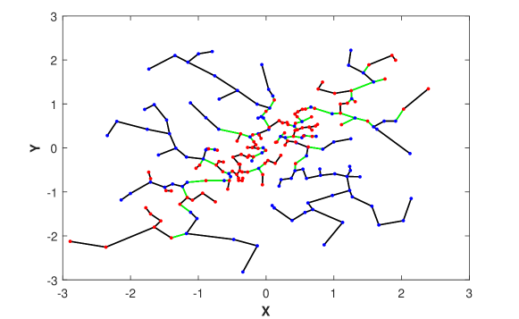
Figure 1: The MST and FR statistic of spanning the merged set of Normal points when 𝐗𝐗\mathbf{X} and 𝐘𝐘\mathbf{Y} are independent (denoted in blue points) and when 𝐗𝐗\mathbf{X} and 𝐘𝐘\mathbf{Y} are highly dependent (denoted in red points). The FR test statistic is the number of edges in the MST that connect samples from different color nodes (denoted in green) and it is used to estimate the GMI Ipsubscript𝐼𝑝I_{p}.

Theorem 2.2 shows that the output in Algorithm 1 estimates the GMI with parameter p=α𝑝𝛼p={\alpha}. The proof is provided in Appendix D, Subsection 5.4. {Theorem} For given proportionality parameter α(0,1)𝛼01\alpha\in(0,1), choose nsuperscript𝑛n^{\prime}, n′′superscript𝑛′′n^{\prime\prime} such that n+n′′=nsuperscript𝑛superscript𝑛′′𝑛n^{\prime}+n^{\prime\prime}=n and as n𝑛n\rightarrow\infty, we have n/nαsuperscript𝑛𝑛𝛼n^{\prime}/n\rightarrow\alpha and n′′/nβ=1αsuperscript𝑛′′𝑛𝛽1𝛼n^{\prime\prime}/n\rightarrow\beta=1-\alpha. Then

1n,n′′(𝒵n,𝒵~n′′)n2nn′′Iα(𝐗;𝐘),a.s.formulae-sequence1subscriptsuperscript𝑛superscript𝑛′′subscriptsuperscript𝒵superscript𝑛subscript~𝒵superscript𝑛′′𝑛2superscript𝑛superscript𝑛′′subscript𝐼𝛼𝐗𝐘𝑎𝑠\displaystyle 1-\mathfrak{R}_{n^{\prime},n^{\prime\prime}}(\mathcal{Z}^{\prime}_{n^{\prime}},\widetilde{\mathcal{Z}}_{n^{\prime\prime}})\;\displaystyle\frac{n}{2n^{\prime}\;n^{\prime\prime}}\rightarrow I_{\alpha}(\mathbf{X};\mathbf{Y}),\;\;\;a.s. (14)

Note that the asymptotic limit in (14) depends on the proportionality parameter α𝛼\alpha. Later in Subsection 2.4, we discuss on choosing an optimal parameter α~~𝛼\tilde{\alpha}. In Fig. 1, we show a visualization of the MST constructed over merged independent (ρ=0𝜌0\rho=0) and highly dependent (ρ=0.9𝜌0.9\rho=0.9) data sets drawn from two dimensional standard Normal distribution with correlation coefficient ρ𝜌\rho. Notice that the MST connects different colored samples, corresponding to independent and dependent samples, respectively, indicated in green. The total number of green edges is the FR test statistic.

2.3 Convergence Rates

In this subsection we provide the MSE convergence rates in the form of upper bounds on the bias and the variance. This MSE bound is given in terms of the sample size n𝑛n, the dimension d𝑑d, and the proportionality parameter α𝛼\alpha. Deriving convergence rates for mutual information estimators has been of interest in information theory and machine learning Pál et al. (2010), Moon et al. (2017). The rates are typically derived in terms of a smoothness condition on the densities, such as the Hölder condition Wolfgang (1991). Here we assume fXsubscript𝑓𝑋f_{X}, fYsubscript𝑓𝑌f_{Y} and fXYsubscript𝑓𝑋𝑌f_{XY} with support sets 𝕊Xsubscript𝕊𝑋\mathbb{S}_{X}, 𝕊Ysubscript𝕊𝑌\mathbb{S}_{Y}, and 𝕊XY:=𝕊X×𝕊Yassignsubscript𝕊𝑋𝑌subscript𝕊𝑋subscript𝕊𝑌\mathbb{S}_{XY}:=\mathbb{S}_{X}\times\mathbb{S}_{Y}, respectively, are smooth in the sense that they belong to strong Hölder continuous classes of densities Σds(η,\Sigma^{s}_{d}(\eta, K), 0<η10𝜂10<\eta\leq 1 Lorentz (1966), Wolfgang (1991): {Definition} (Strong Hölder class): Let 𝒳d𝒳superscript𝑑\mathcal{X}\subset{\mathbb{R}}^{d} be a compact space. The strong Hölder class Σds(η,K)superscriptsubscriptΣ𝑑𝑠𝜂𝐾\Sigma_{d}^{s}(\eta,K), with η𝜂\eta-Hölder parameter and constant K𝐾K, of functions on Ldsubscript𝐿𝑑L_{d}-norm, consists of the functions g𝑔g that satisfy

{g:g(𝐳)p𝐱η(𝐳)dKg(𝐱)𝐱𝐳dη,𝐱,𝐳𝒳},conditional-set𝑔formulae-sequencesubscriptnorm𝑔𝐳superscriptsubscript𝑝𝐱𝜂𝐳𝑑𝐾𝑔𝐱superscriptsubscriptnorm𝐱𝐳𝑑𝜂𝐱𝐳𝒳\displaystyle\begin{array}[]{l}\Big{\{}g:\big{\|}g(\mathbf{z})-p_{\mathbf{x}}^{\lfloor\eta\rfloor}(\mathbf{z})\big{\|}_{d}\leq K\;g(\mathbf{x})\;\big{\|}\mathbf{x}-\mathbf{z}\big{\|}_{d}^{\eta},\;\;\mathbf{x},\;\mathbf{z}\in\mathcal{X}\Big{\}},\end{array} (16)

where p𝐱k(𝐳)superscriptsubscript𝑝𝐱𝑘𝐳p_{\mathbf{x}}^{k}(\mathbf{z}) is the Taylor polynomial (multinomial) of g𝑔g of order k𝑘k expanded about the point 𝐱𝐱\mathbf{x} and η𝜂\lfloor\eta\rfloor is defined as the greatest integer strictly less than η𝜂\eta. Note that for the standard Hölder class the factor g(𝐱)𝑔𝐱g(\mathbf{x}) on the RHS of (16) is omitted. To find the optimal parameter α𝛼\alpha we require explicit expressions for the bias and variance. Bounds are provided in Appendix E, Subsection 5.5. To obtain such expressions, we require several assumptions on the absolutely continuous densities fXsubscript𝑓𝑋f_{X}, fYsubscript𝑓𝑌f_{Y}, fXYsubscript𝑓𝑋𝑌f_{XY} and support sets 𝕊Xsubscript𝕊𝑋\mathbb{S}_{X}, 𝕊Ysubscript𝕊𝑌\mathbb{S}_{Y}, 𝕊XYsubscript𝕊𝑋𝑌\mathbb{S}_{XY}:

  • (A.1)

    Each of the densities belong to Σds(η,K)subscriptsuperscriptΣ𝑠𝑑𝜂𝐾\displaystyle\Sigma^{s}_{d}(\eta,K) class in their support sets with smoothness parameters η𝜂\eta and smoothness constants K𝐾K.

  • (A.2)

    The volumes of the support sets are finite, i.e. 0<𝕍(𝕊X)<,   0<𝕍(𝕊Y)<formulae-sequence0𝕍subscript𝕊𝑋   0𝕍subscript𝕊𝑌0<\mathbb{V}(\mathbb{S}_{X})<\infty,\;\;\;0<\mathbb{V}(\mathbb{S}_{Y})<\infty.

  • (A.3)

    All densities are bounded on their support sets, i.e. there exist two sets of constants CXL,CYL,CXYLsubscriptsuperscript𝐶𝐿𝑋subscriptsuperscript𝐶𝐿𝑌subscriptsuperscript𝐶𝐿𝑋𝑌C^{L}_{X},C^{L}_{Y},C^{L}_{XY} and CXU,CYU,CXYUsubscriptsuperscript𝐶𝑈𝑋subscriptsuperscript𝐶𝑈𝑌subscriptsuperscript𝐶𝑈𝑋𝑌C^{U}_{X},C^{U}_{Y},C^{U}_{XY} such that 0<CXLfXCXU<0subscriptsuperscript𝐶𝐿𝑋subscript𝑓𝑋subscriptsuperscript𝐶𝑈𝑋0<C^{L}_{X}\leq f_{X}\leq C^{U}_{X}<\infty, 0<CYLfYCYU<0subscriptsuperscript𝐶𝐿𝑌subscript𝑓𝑌subscriptsuperscript𝐶𝑈𝑌0<C^{L}_{Y}\leq f_{Y}\leq C^{U}_{Y}<\infty and 0<CXYLfXYCXYU<0subscriptsuperscript𝐶𝐿𝑋𝑌subscript𝑓𝑋𝑌subscriptsuperscript𝐶𝑈𝑋𝑌0<C^{L}_{XY}\leq f_{XY}\leq C^{U}_{XY}<\infty.

Remarks:

  • 1.

    The assumption (A.3) implies that the strong Hölder class, (A.1), is a subset of standard Hölder class:

    {g:g(𝐳)p𝐱η(𝐳)dK𝐱𝐳dη,𝐱,𝐳𝒳}.conditional-set𝑔formulae-sequencesubscriptnorm𝑔𝐳superscriptsubscript𝑝𝐱𝜂𝐳𝑑superscript𝐾superscriptsubscriptnorm𝐱𝐳𝑑𝜂𝐱𝐳𝒳\Big{\{}g:\big{\|}g(\mathbf{z})-p_{\mathbf{x}}^{\lfloor\eta\rfloor}(\mathbf{z})\big{\|}_{d}\leq K^{\prime}\;\big{\|}\mathbf{x}-\mathbf{z}\big{\|}_{d}^{\eta},\;\;\mathbf{x},\;\mathbf{z}\in\mathcal{X}\Big{\}}. (17)
  • 2.

    If in (A.3) CXL,CYL,CXYLsubscriptsuperscript𝐶𝐿𝑋subscriptsuperscript𝐶𝐿𝑌subscriptsuperscript𝐶𝐿𝑋𝑌C^{L}_{X},C^{L}_{Y},C^{L}_{XY} and CXU,CYU,CXYUsubscriptsuperscript𝐶𝑈𝑋subscriptsuperscript𝐶𝑈𝑌subscriptsuperscript𝐶𝑈𝑋𝑌C^{U}_{X},C^{U}_{Y},C^{U}_{XY} are equal i.e. the density functions are uniform, g(𝐱)=K′′𝑔𝐱superscript𝐾′′g(\mathbf{x})=K^{\prime\prime}, and if K=K.K′′formulae-sequencesuperscript𝐾𝐾superscript𝐾′′K^{\prime}=K.K^{\prime\prime} then two classes (16) and (17) are equal.

  • 3.

    By using the Strong Hölder class (16) our proposed bias bound in Theorem 2.3 below, becomes tighter. Another bound can be derived for the standard Hölder class (17) but the proposed bias bound becomes weaker, and so in the result for bounding convergence rate.

The following theorems on the bias and variance follow under assumptions (A.1), (A.2), and (A.3): {Theorem} Under two assumptions (A.1) and (A.3), for given α(0,1)𝛼01\alpha\in(0,1), β=1α𝛽1𝛼\beta=1-\alpha, the bias of the n,n′′subscriptsuperscript𝑛superscript𝑛′′\mathfrak{R}_{n^{\prime},n^{\prime\prime}} estimator for d2𝑑2d\geq 2, 0<η10𝜂10<\eta\leq 1 satisfies

|𝔼[n,n′′]n2αβf𝐗𝐘(𝐱,𝐲)f𝐗(𝐱)f𝐘(𝐲)αf𝐗𝐘(𝐱,𝐲)+βf𝐗(𝐱)f𝐘(𝐲)d𝐱d𝐲|O(max{nη2/(d(1+η)),(βn)η/(1+η),cd2dn1}),𝔼delimited-[]subscriptsuperscript𝑛superscript𝑛′′𝑛2𝛼𝛽double-integralsubscript𝑓𝐗𝐘𝐱𝐲subscript𝑓𝐗𝐱subscript𝑓𝐘𝐲𝛼subscript𝑓𝐗𝐘𝐱𝐲𝛽subscript𝑓𝐗𝐱subscript𝑓𝐘𝐲differential-d𝐱differential-d𝐲missing-subexpressionabsent𝑂superscript𝑛superscript𝜂2𝑑1𝜂superscript𝛽𝑛𝜂1𝜂subscript𝑐𝑑superscript2𝑑superscript𝑛1\begin{array}[]{l}\displaystyle\bigg{|}\frac{{\mathbb{E}}\big{[}\mathfrak{R}_{n^{\prime},n^{\prime\prime}}\big{]}}{n}-2\alpha\beta\iint\frac{f_{\mathbf{X}\mathbf{Y}}(\mathbf{x},\mathbf{y})f_{\mathbf{X}}(\mathbf{x})f_{\mathbf{Y}}(\mathbf{y})}{\alpha f_{\mathbf{X}\mathbf{Y}}(\mathbf{x},\mathbf{y})+\beta f_{\mathbf{X}}(\mathbf{x})f_{\mathbf{Y}}(\mathbf{y})}\;{\rm d}\mathbf{x}{\rm d}\mathbf{y}\bigg{|}\\ \\ \qquad\quad\leq O\bigg{(}\max\Big{\{}n^{-\eta^{2}\big{/}(d(1+\eta))},\;(\beta n)^{-\eta/(1+\eta)},\;c_{d}2^{d}n^{-1}\Big{\}}\bigg{)},\end{array} (18)

where cdsubscript𝑐𝑑c_{d} is a constant depending only on d𝑑d. Note that according to Theorem 13 in Robins and Salowe (1994), the constant cdsubscript𝑐𝑑c_{d} is lower bounded by Ω(d2n(1H(γ)))Ω𝑑superscript2𝑛1𝐻𝛾\Omega\left(\sqrt{d}2^{n(1-H(\gamma))}\right), γ=2d𝛾superscript2𝑑\gamma=2^{-d} and H(γ)𝐻𝛾H(\gamma) is the binary entropy i.e.

H(γ)=γlogγ(1γ)log(1γ).𝐻𝛾𝛾𝛾1𝛾1𝛾H(\gamma)=-\gamma\log\gamma-(1-\gamma)\log(1-\gamma).

A proof of Theorem 2.3 is given in Appendix E. The next theorem gives an upper bound on the variance of the FR estimator n,n′′subscriptsuperscript𝑛superscript𝑛′′\mathfrak{R}_{n^{\prime},n^{\prime\prime}}. The proof of the variance result requires a different approach than the bias bound. The proof uses the Efron-Stein inequality Efron and stein (1981) and is similar to arguments in (Yasaei Sekeh et al., 2018, Appendix C), and is omitted. In Theorem 2.3 we assume that the densities fXsubscript𝑓𝑋f_{X}, fYsubscript𝑓𝑌f_{Y}, and fXYsubscript𝑓𝑋𝑌f_{XY} are absolutely continuous and bounded. Note that we can obtain a weaker bound than (18) when we relax (A.1) to the standard Hölder class with a constant coefficient Ksuperscript𝐾K^{\prime} instead of Kg(𝐱)𝐾𝑔𝐱Kg(\mathbf{x}). {Theorem} Given α(0,1)𝛼01\alpha\in(0,1), the variance of the estimator n,n′′(𝒵n,𝒵~n′′)subscriptsuperscript𝑛superscript𝑛′′subscriptsuperscript𝒵superscript𝑛subscript~𝒵superscript𝑛′′\mathfrak{R}_{n^{\prime},n^{\prime\prime}}(\mathcal{Z}^{\prime}_{n^{\prime}},\widetilde{\mathcal{Z}}_{n^{\prime\prime}}) is bounded by

Var(n,n′′n)(1α)cdn,α=n/n,formulae-sequence𝑉𝑎𝑟subscriptsuperscript𝑛superscript𝑛′′𝑛1𝛼subscript𝑐𝑑𝑛𝛼superscript𝑛𝑛\displaystyle Var\left(\displaystyle\frac{\mathfrak{R}_{n^{\prime},n^{\prime\prime}}}{n}\right)\leq\displaystyle\frac{{(1-\alpha)\;c_{d}}}{n},\;\;\;\alpha=n^{\prime}/n, (19)

where cdsubscript𝑐𝑑c_{d} is a constant depending only on the dimension d𝑑d.

2.4 Minimax Parameter α𝛼\alpha

A question in Algorithm 1 is the existance of a best proportion α𝛼\alpha that partitions sample. In this subsection we obtain on an upper bound of the MSE rate and characterize the parameter α𝛼\alpha that minimizes the upper bound. This optimal α𝛼\alpha depends on maximize densities, however.

Recall assumptions (A.1), (A.2), and (A.3) in Subsection 2.3. The constant α𝛼\alpha can be chosen to ensure that the MSE converges rate obtained from the bias and variance rates (18) and (2.3) by selecting α𝛼\alpha to minimize the maximum MSE, where the maximum is taken over the space of Hölder smooth joint densities fXYsubscript𝑓𝑋𝑌f_{XY}.

Throughout this subsection we use the following notations:

  • ϵXY:=fXY/fXfYassignsubscriptitalic-ϵ𝑋𝑌subscript𝑓𝑋𝑌subscript𝑓𝑋subscript𝑓𝑌\epsilon_{XY}:=f_{XY}\big{/}f_{X}f_{Y},

  • CϵL:=CXYL/CXUCYUassignsubscriptsuperscript𝐶𝐿italic-ϵsubscriptsuperscript𝐶𝐿𝑋𝑌subscriptsuperscript𝐶𝑈𝑋subscriptsuperscript𝐶𝑈𝑌C^{L}_{\epsilon}:=C^{L}_{XY}\big{/}C^{U}_{X}C^{U}_{Y} and CϵU:=CXYU/CXLCYLassignsubscriptsuperscript𝐶𝑈italic-ϵsubscriptsuperscript𝐶𝑈𝑋𝑌subscriptsuperscript𝐶𝐿𝑋subscriptsuperscript𝐶𝐿𝑌C^{U}_{\epsilon}:=C^{U}_{XY}\big{/}C^{L}_{X}C^{L}_{Y},

  • Cn:=CXYLn/2assignsubscript𝐶𝑛subscriptsuperscript𝐶𝐿𝑋𝑌𝑛2C_{n}:=C^{L}_{XY}\;n/2,

  • α0L:=2Cnassignsubscriptsuperscript𝛼𝐿02subscript𝐶𝑛\alpha^{L}_{0}:=\displaystyle\frac{2}{C_{n}} and α0U:=min{14,1+1/Cn4+2CϵU,1nη/d1}assignsubscriptsuperscript𝛼𝑈01411subscript𝐶𝑛42subscriptsuperscript𝐶𝑈italic-ϵ1superscript𝑛𝜂𝑑1\alpha^{U}_{0}:=\min\left\{\displaystyle\frac{1}{4},\displaystyle\frac{1+1/C_{n}}{4+2C^{U}_{\epsilon}},1-n^{\eta/d-1}\right\}, where η𝜂\eta is the smoothness parameter,

  • ln:=nη/(d2(1+η))assignsubscript𝑙𝑛superscript𝑛𝜂superscript𝑑21𝜂l_{n}:=\big{\lfloor}n^{\eta/(d^{2}(1+\eta))}\big{\rfloor}.

Now define G~ϵXY,nα,β(𝐱,𝐲)subscriptsuperscript~𝐺𝛼𝛽subscriptitalic-ϵ𝑋𝑌𝑛𝐱𝐲\widetilde{{G}}^{\alpha,\beta}_{\epsilon_{XY},n}(\mathbf{x},\mathbf{y}) by

(ϵXY(𝐱,𝐲)+1/(βCn))(1+ϵXY(𝐱𝐲)+1/(βCn))(α+βϵXY(𝐱,𝐲))2,β=1α.subscriptitalic-ϵ𝑋𝑌𝐱𝐲1𝛽subscript𝐶𝑛1subscriptitalic-ϵ𝑋𝑌𝐱𝐲1𝛽subscript𝐶𝑛superscript𝛼𝛽subscriptitalic-ϵ𝑋𝑌𝐱𝐲2𝛽1𝛼\displaystyle\frac{(\epsilon_{XY}(\mathbf{x},\mathbf{y})+1/(\beta C_{n}))(1+\epsilon_{XY}(\mathbf{x}\mathbf{y})+1/(\beta C_{n}))}{(\alpha+\beta\epsilon_{XY}(\mathbf{x},\mathbf{y}))^{2}},\;\;\;\beta=1-\alpha. (20)

Consider the following optimization problem:

min𝛼maxϵXY𝛼minsubscriptitalic-ϵ𝑋𝑌max\displaystyle\underset{\alpha}{\text{min}}\;\;\underset{\epsilon_{XY}}{\text{max}} Δ~(α,ϵXY)+cd(1α)n1~Δ𝛼subscriptitalic-ϵ𝑋𝑌subscript𝑐𝑑1𝛼superscript𝑛1\displaystyle\widetilde{\Delta}(\alpha,\epsilon_{XY})+c_{d}(1-\alpha)\;n^{-1} (21)
subject to CϵLϵXYCϵU,subscriptsuperscript𝐶𝐿italic-ϵsubscriptitalic-ϵ𝑋𝑌subscriptsuperscript𝐶𝑈italic-ϵ\displaystyle C^{L}_{\epsilon}\leq\epsilon_{XY}\leq C^{U}_{\epsilon},
α0Lαα0U,subscriptsuperscript𝛼𝐿0𝛼subscriptsuperscript𝛼𝑈0\displaystyle\alpha^{L}_{0}\leq\alpha\leq\alpha^{U}_{0},

where

Δ~(α,ϵXY):=D(n,ln,d,η)+D¯(n,ln,d)CXYU𝕊XYG~ϵXY,nα,β(𝐱,𝐲)d𝐱d𝐲,assign~Δ𝛼subscriptitalic-ϵ𝑋𝑌𝐷𝑛subscript𝑙𝑛𝑑𝜂¯𝐷𝑛subscript𝑙𝑛𝑑subscriptsuperscript𝐶𝑈𝑋𝑌subscriptdouble-integralsubscript𝕊𝑋𝑌subscriptsuperscript~𝐺𝛼𝛽subscriptitalic-ϵ𝑋𝑌𝑛𝐱𝐲differential-d𝐱differential-d𝐲\displaystyle\widetilde{\Delta}(\alpha,\epsilon_{XY}):=\displaystyle D(n,l_{n},d,\eta)+\overline{D}(n,l_{n},d)C^{U}_{XY}\displaystyle\iint_{\mathbb{S}_{XY}}\widetilde{{G}}^{\alpha,\beta}_{\epsilon_{XY},n}(\mathbf{x},\mathbf{y})\;{\rm d}\mathbf{x}{\rm d}\mathbf{y}, (22)

and

D(n,ln,d,η)=c2lndn1+cd2dn1+clndnη/d+clndn1/d+2c1lnd1n1/d1,𝐷𝑛subscript𝑙𝑛𝑑𝜂subscript𝑐2superscriptsubscript𝑙𝑛𝑑superscript𝑛1subscript𝑐𝑑superscript2𝑑superscript𝑛1superscript𝑐superscriptsubscript𝑙𝑛𝑑superscript𝑛𝜂𝑑𝑐superscriptsubscript𝑙𝑛𝑑superscript𝑛1𝑑2subscript𝑐1superscriptsubscript𝑙𝑛𝑑1superscript𝑛1𝑑1\displaystyle\begin{array}[]{l}D(n,l_{n},d,\eta)=\displaystyle c_{2}l_{n}^{d}n^{-1}+c_{d}2^{d}n^{-1}+c^{\prime}l_{n}^{d}n^{-\eta/d}+\displaystyle cl_{n}^{d}n^{-1/d}+2c_{1}l_{n}^{d-1}n^{1/d-1},\end{array} (24)
D~(n,ln,d)=2+n12c′′i=1Mlnlndai1+n3/22c1i=1Mlnlnd/2biai2+n1i=1M2n3/2lnd/2biai2(nailnd+n2ai2)1/2(nbilnd+n2bi2)1/2.~𝐷𝑛subscript𝑙𝑛𝑑2superscript𝑛12superscript𝑐′′superscriptsubscript𝑖1𝑀subscript𝑙𝑛superscriptsubscript𝑙𝑛𝑑superscriptsubscript𝑎𝑖1superscript𝑛322subscriptsuperscript𝑐1superscriptsubscript𝑖1𝑀subscript𝑙𝑛superscriptsubscript𝑙𝑛𝑑2subscript𝑏𝑖superscriptsubscript𝑎𝑖2superscript𝑛1superscriptsubscript𝑖1𝑀2superscript𝑛32superscriptsubscript𝑙𝑛𝑑2subscript𝑏𝑖superscriptsubscript𝑎𝑖2superscript𝑛subscript𝑎𝑖superscriptsubscript𝑙𝑛𝑑superscript𝑛2superscriptsubscript𝑎𝑖212superscript𝑛subscript𝑏𝑖superscriptsubscript𝑙𝑛𝑑superscript𝑛2superscriptsubscript𝑏𝑖212\begin{array}[]{l}\widetilde{D}(n,l_{n},d)=\displaystyle 2+n^{-1}2c^{\prime\prime}\sum\limits_{i=1}^{M}l_{n}\;l_{n}^{d}a_{i}^{-1}+n^{-3/2}2c^{\prime}_{1}\sum\limits_{i=1}^{M}l_{n}\;l_{n}^{d/2}\sqrt{b_{i}}{a_{i}^{2}}\\ \qquad+n^{-1}\displaystyle\sum\limits_{i=1}^{M}2n^{-3/2}l_{n}^{-d/2}\displaystyle\frac{\sqrt{b_{i}}}{a_{i}^{2}}\big{(}na_{i}l_{n}^{d}+n^{2}a_{i}^{2}\big{)}^{1/2}\big{(}nb_{i}l_{n}^{d}+n^{2}b_{i}^{2}\big{)}^{1/2}.\end{array} (25)

Note that in (24), c,c,c1,c2𝑐superscript𝑐subscript𝑐1subscript𝑐2c,c^{\prime},c_{1},c_{2} are constants, and cdsubscript𝑐𝑑c_{d} only depends on the dimension d𝑑d. Also, in (25), aisubscript𝑎𝑖a_{i} and bisubscript𝑏𝑖b_{i} are constants. Let ϵXYsuperscriptsubscriptitalic-ϵ𝑋𝑌\epsilon_{XY}^{*} be the optimal ϵXYsubscriptitalic-ϵ𝑋𝑌\epsilon_{XY} i.e. ϵXYsuperscriptsubscriptitalic-ϵ𝑋𝑌\epsilon_{XY}^{*} be the solution of the optimization problem (21). Set

Ξ(α):=ddα(Δ~(α,ϵXY)+cd(1α)n1),assignΞ𝛼dd𝛼~Δ𝛼subscriptsuperscriptitalic-ϵ𝑋𝑌subscript𝑐𝑑1𝛼superscript𝑛1\begin{array}[]{l}\Xi(\alpha):=\displaystyle\frac{{\rm d}}{{\rm d}\alpha}\Big{(}\widetilde{\Delta}(\alpha,\epsilon^{*}_{XY})+c_{d}(1-\alpha)\;n^{-1}\Big{)},\\ \end{array} (26)

such that Δ~(α,ϵXY)~Δ𝛼subscriptsuperscriptitalic-ϵ𝑋𝑌\displaystyle\widetilde{\Delta}(\alpha,\epsilon^{*}_{XY}) is (22) when ϵXY=ϵXYsubscriptitalic-ϵ𝑋𝑌subscriptsuperscriptitalic-ϵ𝑋𝑌\epsilon_{XY}=\epsilon^{*}_{XY}. For α[α0L,α0U\alpha\in[\alpha^{L}_{0},\alpha^{U}_{0}], the optimal choice of ϵXYsubscriptitalic-ϵ𝑋𝑌\epsilon_{XY} in terms of maximizing the MSE is ϵXY=CϵUsuperscriptsubscriptitalic-ϵ𝑋𝑌subscriptsuperscript𝐶𝑈italic-ϵ\epsilon_{XY}^{*}=C^{U}_{\epsilon} and the saddle point for the parameter α𝛼\alpha, denoted by α~~𝛼\tilde{\alpha}, is given as follows:

  • α~=α0U~𝛼superscriptsubscript𝛼0𝑈\tilde{\alpha}=\alpha_{0}^{U}, if Ξ(α0U)<0Ξsuperscriptsubscript𝛼0𝑈0\Xi(\alpha_{0}^{U})<0.

  • α~=α0L~𝛼superscriptsubscript𝛼0𝐿\tilde{\alpha}=\alpha_{0}^{L}, if Ξ(α0L)>0Ξsuperscriptsubscript𝛼0𝐿0\Xi(\alpha_{0}^{L})>0.

  • α~=Ξ1(0)~𝛼superscriptΞ10\tilde{\alpha}=\Xi^{-1}(0), if α0LΞ1(0)α0Usuperscriptsubscript𝛼0𝐿superscriptΞ10superscriptsubscript𝛼0𝑈\alpha_{0}^{L}\leq\Xi^{-1}(0)\leq\alpha_{0}^{U}.

Further details are given in Appendix F.

3 Simulation Study

In this section numerical simulations are presented that illustrate the theory in Section 2. We perform multiple experiments to demonstrate the utility of the proposed direct estimator of the HP-divergence in terms of the dimension d𝑑d and the sample size n𝑛n. Our proposed MST-based estimator of the GMI is compared to other plug-in GMI estimators, in particular the standard KDE estimator of Moon et al. (2017), where the convergence rates of Theorem 2.3 and 2.3 are validated. We use multivariate Normal simulated data in the experiments. In this section, we also discuss the choice of the proportionality parameter α𝛼\alpha and compare runtime of our proposed FR estimator approach with KDE method.

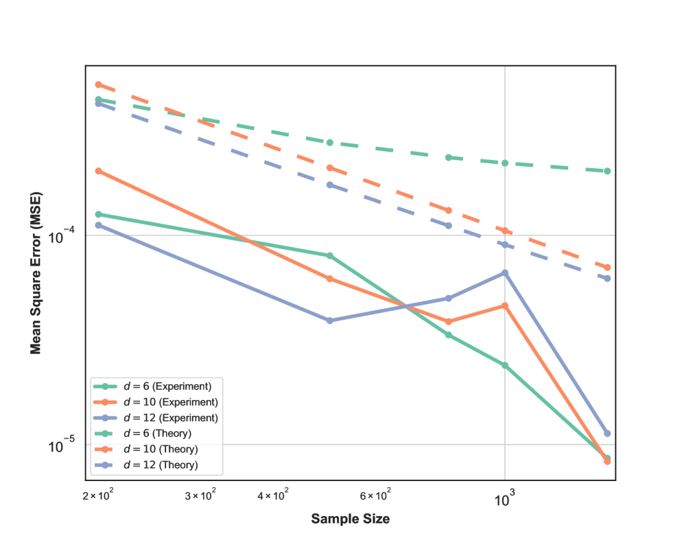
Here we perform four sets of experiments to illustrate the estimator and the theory derived above. For the first set of experiments the MSE of the FR estimator proposed in Algorithm 1 is shown in Fig. 2-(left). The samples were drawn from d𝑑d-dimensional Normal distribution, with various sample sizes and dimensions d=6,10,12𝑑61012d=6,10,12. We selected the proportionality parameter α=0.3𝛼0.3\alpha=0.3 and computed the MSE in terms of the sample size n𝑛n. We show the log-log plot of MSE when n𝑛n varies in [100,1500]1001500[100,1500]. Note that the empirically optimal proportion α𝛼\alpha depends on n𝑛n, so to avoid the computational complexity we fixed α𝛼\alpha for this experiment. The experimental result shown in Fig. 2-(left) validates the theoretical MSE growth rates derived from (18) and (19), i.e., decreasing sublinearly in n𝑛n and increasing exponentially in d𝑑d.

Refer to caption
Refer to caption
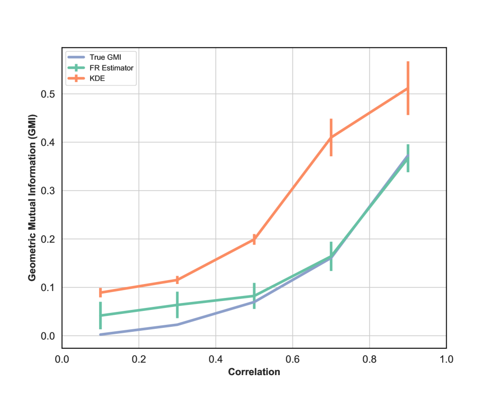
Figure 2: (left) Log–log plot of theoretical and experimental MSE of the FR estimator of the GMI as a function of sample size n𝑛n for d=6,10,12𝑑61012d=6,10,12 and fixed smoothness parameter η𝜂\eta. (right) The GMI estimator using two approaches, FR test statistic and KDE method along with True GMI. In this experiment, we generated data from the two dimensional Normal distribution with zero mean and covariance matrix (27) for various ρ[0.1,0.9]𝜌0.10.9\rho\in[0.1,0.9].

In Fig. 2-(right), we compare our estimator with the true GMI and the standard KDE Moon et al. (2017). For the KDE approach, we estimated the joint and marginal densities and then plugged them into the proposed expression (3) in Moon et al. (2017). The bandwidth used for the the KDE plug-in estimator was selected by setting h=n1/(d+1)superscript𝑛1𝑑1h=n^{-1/(d+1)} to minimize the MSE of the plug in estimator. We generated data from the two dimensional Normal distribution with zero mean and covariance matrix

(1ρρ1).1𝜌𝜌1\left(\begin{array}[]{cc}1&\rho\\ \rho&1\end{array}\right). (27)

We varied ρ𝜌\rho in range [0.1,0.9]0.10.9[0.1,0.9] and computed the proposed estimated GMI and the KDE. We used the Monte Carlo method to approximate the integral (2) and compute the GMI measure (labeled True GMI). We see that as ρ𝜌\rho increases the estimated GMI using the FR test statistic outperforms the KDE approach (FR curve approaches to True curve and KDE curve diverges from True curve). In this set of experiments α=0.6𝛼0.6\alpha=0.6.

Refer to caption
Refer to caption
Refer to caption
Refer to caption
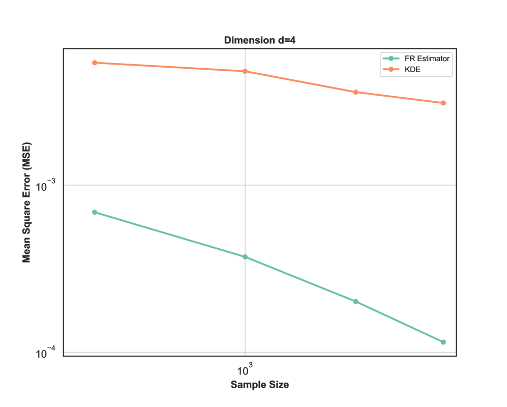
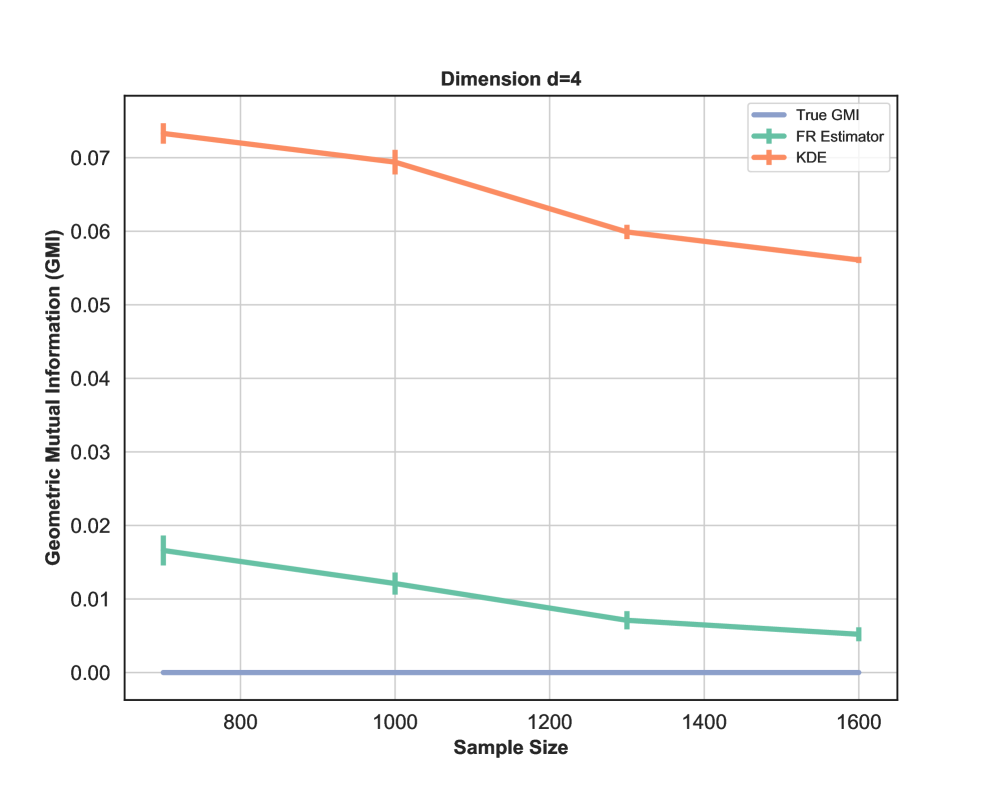
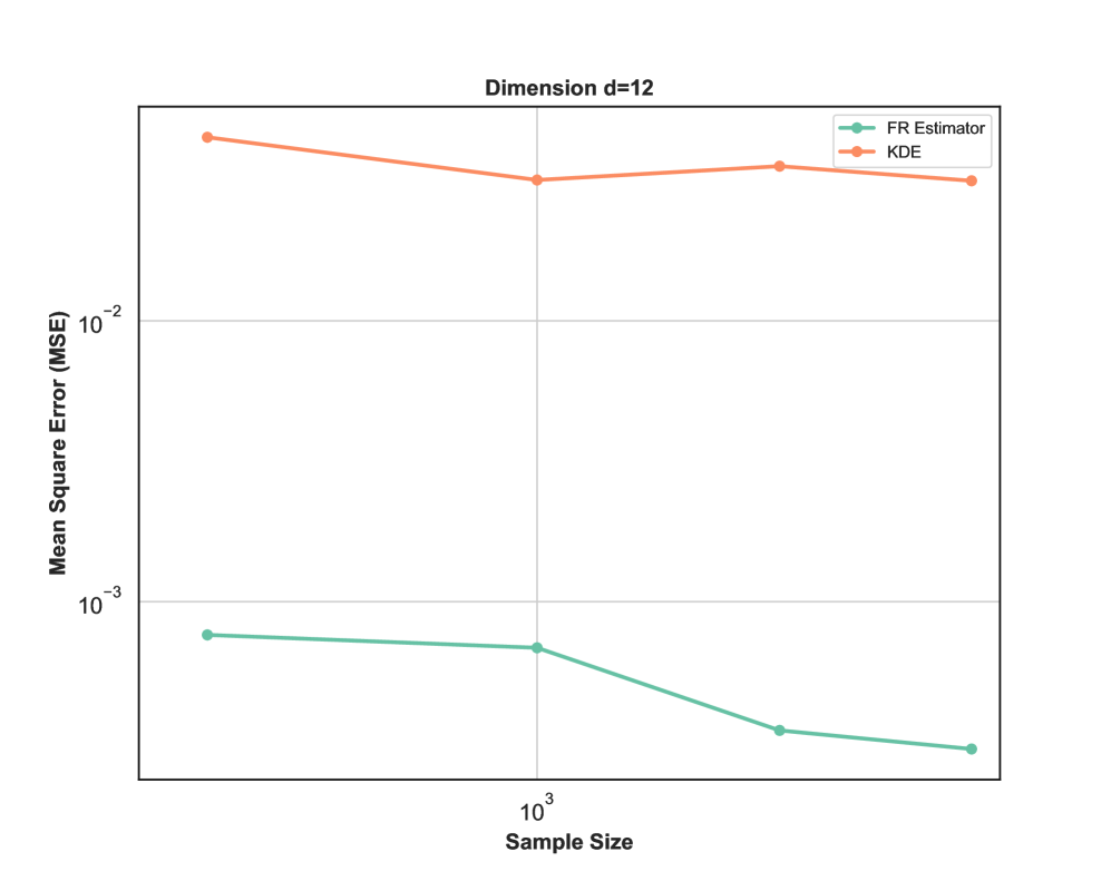
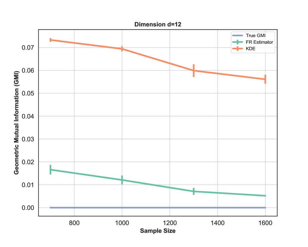
Figure 3: MSE log-log plots as a function of sample size n𝑛n (left) for the proposed Friedman-Rafsky estimator ("Estimated GMI") and the standard KDE plug-in estimator ("KDE"). The two right plots each corresponds to the geometric mutual information with the dimension d=4𝑑4d=4 (top) and d=12𝑑12d=12 (bottom). In both cases the proportionality parameter α𝛼\alpha is 0.50.50.5. The FR estimator in both plots for sample size n𝑛n in [700,1600]7001600[700,1600] outperforms the standard kernel plug-in estimator, especially for larger dimensions.

Fig. 3 again compares the FR estimator with the standard KDE estimator. In this setting, we draw samples from the multivariate standard Normal distribution with dimensions d=4𝑑4d=4 and d=12𝑑12d=12. In both cases the proportionality parameter α=0.5𝛼0.5\alpha=0.5. The left plots in Fig. 3 show the MSE (100 trials) of the GMI estimator implemented with an KDE estimator (with bandwidth as in Fig. 2 i.e. h=n1/(d+1)superscript𝑛1𝑑1h=n^{-1/(d+1)}) for dimensions d=4,12𝑑412d=4,12 and various sample sizes. For all dimensions and sample sizes the FR estimator also outperforms the plug-in KDE estimator based on the estimated log-log MSE slope given in Fig. 3 (left plots). The right plots in Fig. 3 show the geometric mutual information estimated by KED and FR approaches. The iteration in this experiment is 100 and error bars are standard deviations. We observe that for higher dimension d=12𝑑12d=12 and larger sample size n𝑛n, the KDE estimator approaches to the true GMI slower than the FR estimator. This reflects the power of graph-based (direct) estimators, and in particular our proposed FR estimator.
Refer to caption
Refer to caption
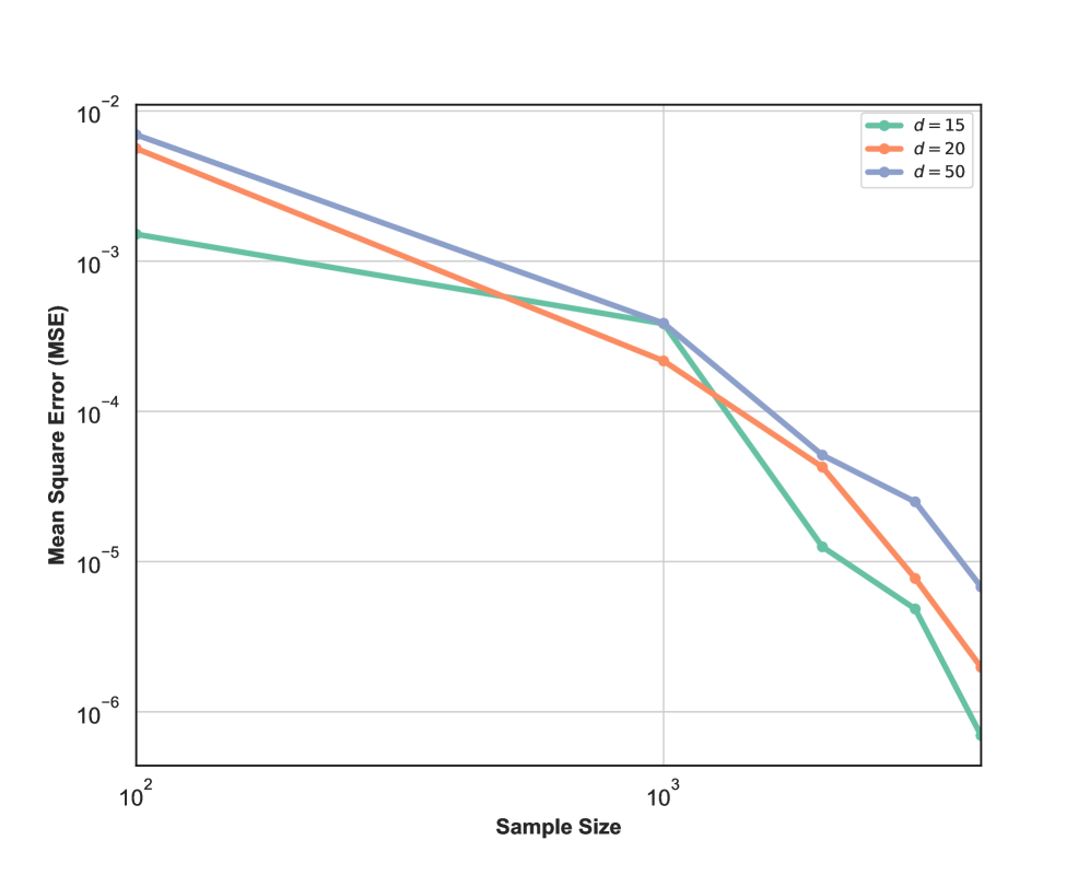
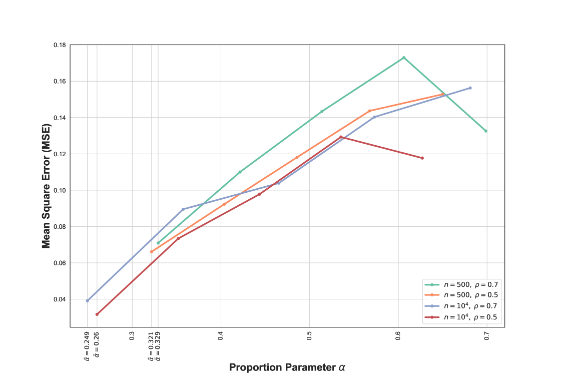
Figure 4: MSE log-log plots as a function of sample size n𝑛n for the proposed FR estimator. We compare the MSE of our proposed FR estimator for various dimensions d=15,20,50𝑑152050d=15,20,50 (left). As d𝑑d increases, the blue curve takes larger values than green and orange curves i.e. MSE increases as d𝑑d grows. However, this is more evidential for large sample size n𝑛n. The second experiment (right) focuses on optimal proportion α𝛼\alpha for n=500,104𝑛500superscript104n=500,10^{4} and ρ=0.7,0.5𝜌0.70.5\rho=0.7,0.5. α~~𝛼\tilde{\alpha} is the optimal α𝛼\alpha for α[α0L,α0U]𝛼superscriptsubscript𝛼0𝐿superscriptsubscript𝛼0𝑈\alpha\in[\alpha_{0}^{L},\alpha_{0}^{U}].

The comparison between MSEs for various dimension d𝑑d is shown in Fig. 4 (left). This experiment highlights higher dimension’s impact on our proposed FR estimator for the GMI measure. As expected, for larger sample size n𝑛n, MSE decreases while for higher dimension it increases. In this setting, we have generated samples from standard Normal distribution with size n[102,4×10³]𝑛superscript1024superscript103n\in[10^{2},4\times 10^{3}] and α=0.5𝛼0.5\alpha=0.5. From Fig. 4 (left) we observe that for larger sample size, MSE curves are ordered based on their corresponding dimensions. Fig. 4 (right) illustrates the MSE vs proportion parameter α𝛼\alpha when n=500,104𝑛500superscript104n=500,10^{4} samples are generated from Normal distribution with ρ=0.7,0.5𝜌0.70.5\rho=0.7,0.5. First, following subsection 2.4, we compute the bound [α0L,α0U]superscriptsubscript𝛼0𝐿superscriptsubscript𝛼0𝑈[\alpha_{0}^{L},\alpha_{0}^{U}] and then derive optimal α𝛼\alpha in this range. Therefore, each experiment with different sample size and ρ𝜌\rho provides different range [α0L,α0U]superscriptsubscript𝛼0𝐿superscriptsubscript𝛼0𝑈[\alpha_{0}^{L},\alpha_{0}^{U}]. We observe that the MSE is not necessarily a monotonic function in α𝛼\alpha and its behavior strongly depends on sample size n𝑛n, d𝑑d, and density functions’ bounds. This is studied extensively in Appendix F. In this set of experiments Ξ(α0L)>0Ξsuperscriptsubscript𝛼0𝐿0\Xi(\alpha_{0}^{L})>0, therefore following the results in subsection 2.4, we have α~=α0L~𝛼superscriptsubscript𝛼0𝐿\tilde{\alpha}=\alpha_{0}^{L}. The optimal α𝛼\alpha is indicated in the Fig. 4 (right).

Next, we consider three scenarios to analyze parameter α𝛼\alpha. In these scenarios the lower bounds CXL,CYL,CXYLsubscriptsuperscript𝐶𝐿𝑋subscriptsuperscript𝐶𝐿𝑌subscriptsuperscript𝐶𝐿𝑋𝑌C^{L}_{X},\;C^{L}_{Y},\;C^{L}_{XY} and upper bounds CXU,CYU,CXYUsubscriptsuperscript𝐶𝑈𝑋subscriptsuperscript𝐶𝑈𝑌subscriptsuperscript𝐶𝑈𝑋𝑌C^{U}_{X},\;C^{U}_{Y},\;C^{U}_{XY} are unknown, therefore results in Section 2.4 are not applicable. In these set of experiments we varied α𝛼\alpha in the range (0,1)01(0,1) to divide our original sample. We generated sample from the multivariate standard Normal distribution in all three scenarios (all features are independent). Therefore the true GMI is zero and in all scenarios the GMI column is compared with zero. In each scenario we fixed dimension d𝑑d and sample size n𝑛n and varied α=0.2,0.5,0.8𝛼0.20.50.8\alpha=0.2,0.5,0.8. The dimension and sample size in Scenarios 1,2, and 3 are d=6,8,10𝑑6810d=6,8,10 and n=1000,1500,2000𝑛100015002000n=1000,1500,2000, respectively. In Table 1 the last column (α𝛼\alpha) stars the parameter α{0.2,0.5,0.8}𝛼0.20.50.8\alpha\in\{0.2,0.5,0.8\} with the minimum MSE and GMI (Iα)subscript𝐼𝛼(I_{\alpha}) in each scenario. Table 1 shows that in these sets of experiments when α=0.5𝛼0.5\alpha=0.5, the GMI estimator has less MSE (i.e. is more accurate) than when α=0.2𝛼0.2\alpha=0.2 or α=0.8𝛼0.8\alpha=0.8. This experimentally demonstrates that if we split our training data, the proposed Algorithm 1 performs better than α=0.2or 0.8𝛼0.2or0.8\alpha=0.2\;\hbox{or}\;0.8 to estimate the GMI measure.

Overview table for different d𝑑d, n𝑛n, and α𝛼\alpha
Experiments Dimension (d𝑑d) Sample size (n𝑛n) GMI (Iαsubscript𝐼𝛼I_{\alpha}) MSE (×104absentsuperscript104\times 10^{-4}) Parameter (α)\alpha)
Scenario 1-1 6 1000 0.0229 12 0.2
Scenario 1-2 6 1000 0.0143 4.7944 0.5*
Scenario 1-3 6 1000 0.0176 6.3867 0.8
Scenario 2-1 8 1500 0.0246 11 0.2
Scenario 2-2 8 1500 0.0074 1.6053 0.5*
Scenario 2-3 8 1500 0.0137 5.3863 0.8
Scenario 3-1 10 2000 0.0074 2.3604 0.2
Scenario 3-2 10 2000 0.0029 0.54180 0.5*
Scenario 3-3 10 2000 0.0262 11 0.8
Table 1: Comparison between different scenarios of various dimensions and sample sizes in terms of parameter α𝛼\alpha. We applied the FR approach to estimate the GMI (Iαsubscript𝐼𝛼I_{\alpha}) with α=0.2,0.5,0.8𝛼0.20.50.8\alpha=0.2,0.5,0.8. We varied dimension d=6,8,10𝑑6810d=6,8,10 and sample size n=1000,1500,2000𝑛100015002000n=1000,1500,2000 in each scenario. We observe that for α={0.2,0.5,0.8}𝛼0.20.50.8\alpha=\{0.2,0.5,0.8\}, the GMI estimator provides less MSE when α=0.5𝛼0.5\alpha=0.5.
Refer to caption
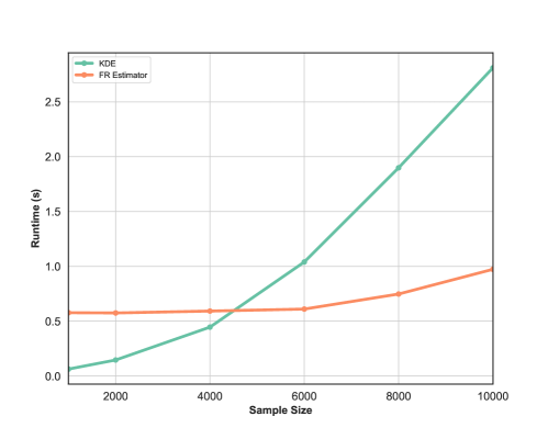
Figure 5: Runtime of KDE approach and proposed FR estimator of GMI measure vs sample size. The proposed GMI estimator achieves significant speedup, while for small sample size, the KDE method becomes overly fast. Note that in this experiment we have generated our sample from standard Gaussian distribution.

Finally Fig. 5 shows the runtime (KDE - FR methods) as a function of sample size n𝑛n. We vary sample size in the range [103,104]superscript103superscript104[10^{3},10^{4}]. Observe that for smaller number of samples the KDE method is slightly faster but as n𝑛n becomes large we see significant relative speedup of the proposed FR method.

4 Conclusion

In this paper we have proposed a new measure of mutual information, called Geometric MI (GMI), that is related to the Henze-Penrose divergence. The GMI can be viewed as dependency measure that is the limit of the Friedman-Rafsky test statistic that depends on the minimal spanning tree over all data points. We established some properties of the GMI in terms of convexity/concavity, chain rule, and analogous to a data processing inequality. A direct estimator of the GMI was introduced that uses random permutations of observed relationships between variables in the multivariate samples. An explicit form for the MSE convergence rate bound was derived that depends on a free parameter called the proportionality parameter. An asymptotically optimal form for this free parameter was given that minimizes the MSE convergence rate. Simulation studies were performed that illustrate and verify the theory.

Acknowledgments

The work presented in this paper was partially supported by ARO grant W911NF-15-1-0479 and DOE grant de-na0002534. The authors would like to thank Brandon Oselio for the useful comments.

5 Appendices

We organize the appendices as the following: Theorem 2.1.1 which establishes convexity/concavity property is proved in Appendix A. Appendix B and C are arranged to establish the inequality (9) and (12) for given p(0,1)𝑝01p\in(0,1), respectively. In Appendix D, we first prove that the set 𝒵~n′′subscript~𝒵superscript𝑛′′\widetilde{\mathcal{Z}}_{n^{\prime\prime}} which is randomly generated from original dependent data, contains independent samples asymptotically. Later by using the generated independent sample 𝒵~n′′subscript~𝒵superscript𝑛′′\widetilde{\mathcal{Z}}_{n^{\prime\prime}} we show that for given α𝛼\alpha the FR estimator of the GMI given in Algorithm 1 intends to Iαsubscript𝐼𝛼I_{\alpha} approximately. Appendix E is dedicated to the Theorem 2.3. A full discussion on the proportionality parameter (α𝛼\alpha) optimization strategy is provided in Appendix F.

5.1 Appendix A: Theorem 2.1.1

Proof.

The proof is similar to the result for standard (Shannon) mutual information. However, we require the following lemma, proved in analogue manner as the log-sum inequality: {Lemma} For non-negative real numbers α1,,αnsubscript𝛼1subscript𝛼𝑛\alpha_{1},\dots,\alpha_{n} and β1,,βnsubscript𝛽1subscript𝛽𝑛\beta_{1},\dots,\beta_{n}, given p(0,1)𝑝01p\in(0,1), q=1p𝑞1𝑝q=1-p, the following holds

i=1nαi(p(βiαi)+q)1i=1nαi(p(i=1nβii=1nαi)+q)1.superscriptsubscript𝑖1𝑛subscript𝛼𝑖superscript𝑝subscript𝛽𝑖subscript𝛼𝑖𝑞1superscriptsubscript𝑖1𝑛subscript𝛼𝑖superscript𝑝superscriptsubscript𝑖1𝑛subscript𝛽𝑖superscriptsubscript𝑖1𝑛subscript𝛼𝑖𝑞1\displaystyle\sum\limits_{i=1}^{n}\alpha_{i}\;\left(p\left(\frac{\beta_{i}}{\alpha_{i}}\right)+q\right)^{-1}\geq\displaystyle\sum\limits_{i=1}^{n}\alpha_{i}\left(p\left(\frac{\sum\limits_{i=1}^{n}\beta_{i}}{\sum\limits_{i=1}^{n}\alpha_{i}}\right)+q\right)^{-1}.

Notice this follows by using the convex function u(y)=y2/(p+qy)𝑢𝑦superscript𝑦2𝑝𝑞𝑦u(y)=\displaystyle y^{2}\big{/}(p+q\;y) for any p(0,1)𝑝01p\in(0,1), q=1p𝑞1𝑝q=1-p, and the Jensen inequality. Define the shorthand 𝐱subscript𝐱\int\limits_{\mathbf{x}}, 𝐲subscript𝐲\int\limits_{\mathbf{y}}, and 𝐱𝐲subscript𝐱𝐲\int\limits_{\mathbf{x}\mathbf{y}} for d𝐱differential-d𝐱\int{\rm d}\mathbf{x}, d𝐲differential-d𝐲\int{\rm d}\mathbf{y} and d𝐱d𝐲double-integraldifferential-d𝐱differential-d𝐲\iint\;{\rm d}\mathbf{x}{\rm d}\mathbf{y}, respectively. To prove part (i) of the Theorem 2.1.1, we represent the LHS of (5) as:

I~p(λ1fY|XgX+λ2fY|XhX)=1𝐱𝐲(λ1fY|XgX+λ2fY|XhX)×[pλ1fY|XgX+λ2fY|XhX(𝐱λ1fY|XgX+λ2fY|XhX)(𝐲λ1fY|XgX+λ2fY|XhX)+q]1=1𝐱𝐲(λ1fY|XgX+λ2fY|XhX)[pfY|X(𝐱λ1fY|XgX+λ2fY|XhX)+q]1.\begin{array}[]{l}\tilde{I}_{p}\big{(}\lambda_{1}f_{Y|X}g_{X}+\lambda_{2}f_{Y|X}h_{X}\big{)}=\displaystyle 1-\displaystyle\int_{\mathbf{x}\mathbf{y}}\left(\lambda_{1}f_{Y|X}g_{X}+\lambda_{2}f_{Y|X}h_{X}\right)\times\\ \\ \displaystyle\left[p\displaystyle\frac{\lambda_{1}f_{Y|X}g_{X}+\lambda_{2}f_{Y|X}h_{X}}{\Big{(}\int_{\mathbf{x}}\lambda_{1}f_{Y|X}g_{X}+\lambda_{2}f_{Y|X}h_{X}\Big{)}\Big{(}\int_{\mathbf{y}}\lambda_{1}f_{Y|X}g_{X}+\lambda_{2}f_{Y|X}h_{X}\Big{)}}+q\right]^{-1}\\ \\ =\displaystyle 1-\int_{\mathbf{x}\mathbf{y}}\left(\lambda_{1}f_{Y|X}g_{X}+\lambda_{2}f_{Y|X}h_{X}\right)\left[p\displaystyle\frac{f_{Y|X}}{\Big{(}\int_{\mathbf{x}}\lambda_{1}f_{Y|X}g_{X}+\lambda_{2}f_{Y|X}h_{X}\Big{)}}+q\right]^{-1}.\end{array}

Furthermore, the RHS of (5) can be rewritten as

λ1I~p(fY|XgX)+λ2I~p(fY|XhX)=1𝐱𝐲(λ1fY|XgX[pfY|XgX(𝐱fY|XgX)(𝐲fY|XgX)+q]1+λ2fY|XhX[pfY|XhX(𝐱fY|XhX)(𝐲fY|XhX)+q]1)=1𝐱𝐲(λ1fY|XgX[pfY|X𝐱fY|XgX+q]1+λ2fY|XhX[pfY|X𝐱fY|XhX+q]1).subscript𝜆1subscript~𝐼𝑝subscript𝑓conditional𝑌𝑋subscript𝑔𝑋subscript𝜆2subscript~𝐼𝑝subscript𝑓conditional𝑌𝑋subscript𝑋missing-subexpressionabsent1subscript𝐱𝐲subscript𝜆1subscript𝑓conditional𝑌𝑋subscript𝑔𝑋superscriptdelimited-[]𝑝subscript𝑓conditional𝑌𝑋subscript𝑔𝑋subscript𝐱subscript𝑓conditional𝑌𝑋subscript𝑔𝑋subscript𝐲subscript𝑓conditional𝑌𝑋subscript𝑔𝑋𝑞1subscript𝜆2subscript𝑓conditional𝑌𝑋subscript𝑋superscriptdelimited-[]𝑝subscript𝑓conditional𝑌𝑋subscript𝑋subscript𝐱subscript𝑓conditional𝑌𝑋subscript𝑋subscript𝐲subscript𝑓conditional𝑌𝑋subscript𝑋𝑞1missing-subexpressionabsent1subscript𝐱𝐲subscript𝜆1subscript𝑓conditional𝑌𝑋subscript𝑔𝑋superscriptdelimited-[]𝑝subscript𝑓conditional𝑌𝑋subscript𝐱subscript𝑓conditional𝑌𝑋subscript𝑔𝑋𝑞1subscript𝜆2subscript𝑓conditional𝑌𝑋subscript𝑋superscriptdelimited-[]𝑝subscript𝑓conditional𝑌𝑋subscript𝐱subscript𝑓conditional𝑌𝑋subscript𝑋𝑞1\begin{array}[]{l}\lambda_{1}\tilde{I}_{p}(f_{Y|X}g_{X})+\lambda_{2}\tilde{I}_{p}(f_{Y|X}h_{X})\\ \\ =\displaystyle 1-\displaystyle\int\limits_{\mathbf{x}\mathbf{y}}\left(\lambda_{1}f_{Y|X}g_{X}\left[p\frac{f_{Y|X}g_{X}}{\big{(}\int\limits_{\mathbf{x}}f_{Y|X}g_{X}\big{)}\big{(}\int\limits_{\mathbf{y}}f_{Y|X}g_{X}\big{)}}+q\right]^{-1}+\displaystyle\lambda_{2}f_{Y|X}h_{X}\left[p\frac{f_{Y|X}h_{X}}{\big{(}\int\limits_{\mathbf{x}}f_{Y|X}h_{X}\big{)}\big{(}\int\limits_{\mathbf{y}}f_{Y|X}h_{X}\big{)}}+q\right]^{-1}\right)\\ \\ \qquad=1-\displaystyle\int\limits_{\mathbf{x}\mathbf{y}}\left(\lambda_{1}f_{Y|X}g_{X}\left[p\frac{f_{Y|X}}{\int\limits_{\mathbf{x}}f_{Y|X}g_{X}}+q\right]^{-1}+\displaystyle\lambda_{2}f_{Y|X}h_{X}\left[p\frac{f_{Y|X}}{\int\limits_{\mathbf{x}}f_{Y|X}h_{X}}+q\right]^{-1}\right).\end{array}

Thus, in order to prove LHSRHSLHSRHS\hbox{LHS}\geq\hbox{RHS}, we use the inequality below:

(λ1fY|XgX+λ2fY|XhX)[pfY|X𝐱λ1fY|XgX+λ2fY|XhX+q]1(λ1fY|XgX)[pπ𝐱fY|XgX+q]1+(λ2fY|XhX)[pπ𝐱fY|XhX+q]1.subscript𝜆1subscript𝑓conditional𝑌𝑋subscript𝑔𝑋subscript𝜆2subscript𝑓conditional𝑌𝑋subscript𝑋superscriptdelimited-[]𝑝subscript𝑓conditional𝑌𝑋subscript𝐱subscript𝜆1subscript𝑓conditional𝑌𝑋subscript𝑔𝑋subscript𝜆2subscript𝑓conditional𝑌𝑋subscript𝑋𝑞1missing-subexpressionabsentsubscript𝜆1subscript𝑓conditional𝑌𝑋subscript𝑔𝑋superscriptdelimited-[]𝑝𝜋subscript𝐱subscript𝑓conditional𝑌𝑋subscript𝑔𝑋𝑞1subscript𝜆2subscript𝑓conditional𝑌𝑋subscript𝑋superscriptdelimited-[]𝑝𝜋subscript𝐱subscript𝑓conditional𝑌𝑋subscript𝑋𝑞1\begin{array}[]{l}\displaystyle\left(\lambda_{1}f_{Y|X}g_{X}+\lambda_{2}f_{Y|X}h_{X}\right)\left[p\frac{f_{Y|X}}{\int\limits_{\mathbf{x}}\lambda_{1}f_{Y|X}g_{X}+\lambda_{2}f_{Y|X}h_{X}}+q\right]^{-1}\\ \\ \quad\qquad\leq\displaystyle\left(\lambda_{1}f_{Y|X}g_{X}\right)\left[p\frac{\pi}{\int\limits_{\mathbf{x}}f_{Y|X}g_{X}}+q\right]^{-1}+\displaystyle\left(\lambda_{2}f_{Y|X}h_{X}\right)\left[p\frac{\pi}{\int\limits_{\mathbf{x}}f_{Y|X}h_{X}}+q\right]^{-1}.\end{array}

In Lemma 5.1, let

α1=λ1(𝐱fY|XgX)(λ1fY|XgX+λ2fY|XhX)𝐱λ1fY|XgX+λ2fY|XhX,α2=λ2(𝐱fY|XhX)(λ1fY|XgX+λ2fY|XhX)𝐱λ1fY|XgX+λ2fY|XhX,subscript𝛼1subscript𝜆1subscript𝐱subscript𝑓conditional𝑌𝑋subscript𝑔𝑋subscript𝜆1subscript𝑓conditional𝑌𝑋subscript𝑔𝑋subscript𝜆2subscript𝑓conditional𝑌𝑋subscript𝑋subscript𝐱subscript𝜆1subscript𝑓conditional𝑌𝑋subscript𝑔𝑋subscript𝜆2subscript𝑓conditional𝑌𝑋subscript𝑋missing-subexpressionmissing-subexpressionmissing-subexpressionmissing-subexpressionmissing-subexpressionsubscript𝛼2subscript𝜆2subscript𝐱subscript𝑓conditional𝑌𝑋subscript𝑋subscript𝜆1subscript𝑓conditional𝑌𝑋subscript𝑔𝑋subscript𝜆2subscript𝑓conditional𝑌𝑋subscript𝑋subscript𝐱subscript𝜆1subscript𝑓conditional𝑌𝑋subscript𝑔𝑋subscript𝜆2subscript𝑓conditional𝑌𝑋subscript𝑋missing-subexpressionmissing-subexpression\begin{array}[]{ccl}\displaystyle\alpha_{1}=\displaystyle\frac{\lambda_{1}\left(\int\limits_{\mathbf{x}}f_{Y|X}g_{X}\right)\left(\lambda_{1}f_{Y|X}g_{X}+\lambda_{2}f_{Y|X}h_{X}\right)}{\int\limits_{\mathbf{x}}\lambda_{1}f_{Y|X}g_{X}+\lambda_{2}f_{Y|X}h_{X}},\\ \\ \displaystyle\alpha_{2}=\displaystyle\frac{\lambda_{2}\left(\int\limits_{\mathbf{x}}f_{Y|X}h_{X}\right)\left(\lambda_{1}f_{Y|X}g_{X}+\lambda_{2}f_{Y|X}h_{X}\right)}{\int\limits_{\mathbf{x}}\lambda_{1}f_{Y|X}g_{X}+\lambda_{2}f_{Y|X}h_{X}},\end{array}

and for i=1,2𝑖12i=1,2,

βi=λifY|X(λ1fY|XgX+λ2fY|XhX)𝐱λ1fY|XgX+λ2fY|XhX.subscript𝛽𝑖subscript𝜆𝑖subscript𝑓conditional𝑌𝑋subscript𝜆1subscript𝑓conditional𝑌𝑋subscript𝑔𝑋subscript𝜆2subscript𝑓conditional𝑌𝑋subscript𝑋subscript𝐱subscript𝜆1subscript𝑓conditional𝑌𝑋subscript𝑔𝑋subscript𝜆2subscript𝑓conditional𝑌𝑋subscript𝑋\beta_{i}=\displaystyle\frac{\lambda_{i}f_{Y|X}\Big{(}\lambda_{1}f_{Y|X}g_{X}+\lambda_{2}f_{Y|X}h_{X}\Big{)}}{\int\limits_{\mathbf{x}}\lambda_{1}f_{Y|X}g_{X}+\lambda_{2}f_{Y|X}h_{X}}.

Then the claimed assertion (i) is obtained. Part (ii) follows by convexity of Dpsubscript𝐷𝑝D_{p} and the following expression:

I~p(λ1gY|XfX+λ2hY|XfX)=Dp(λ1fXgY|X+λ2fXhY|X,(𝐱λ1fXgY|X+λ2fXhY|X)(𝐲λ1ϕπ1+λ2ϕπ2))=Dp(λ1fXgY|X+λ2fXhY|X,fX(𝐱λ1fXgY|X+λ2fXhY|X)=Dp(λ1fXgY|X+λ2fXhY|X,λ1(𝐱fXgY|X)(𝐲fXgY|X)+λ2(𝐱fXhY|X)(𝐲fXhY|X)).\begin{array}[]{l}\tilde{I}_{p}\big{(}\lambda_{1}g_{Y|X}f_{X}+\lambda_{2}h_{Y|X}f_{X}\big{)}\\ \\ \qquad=\displaystyle D_{p}\bigg{(}\lambda_{1}f_{X}g_{Y|X}+\lambda_{2}f_{X}h_{Y|X}\;,\bigg{(}\int\limits_{\mathbf{x}}\lambda_{1}f_{X}g_{Y|X}+\lambda_{2}f_{X}h_{Y|X}\bigg{)}\displaystyle\bigg{(}\int\limits_{\mathbf{y}}\lambda_{1}\phi\pi_{1}+\lambda_{2}\phi\pi_{2}\bigg{)}\bigg{)}\\ \qquad=\displaystyle D_{p}\bigg{(}\lambda_{1}f_{X}g_{Y|X}+\lambda_{2}f_{X}h_{Y|X}\;,f_{X}\bigg{(}\int\limits_{\mathbf{x}}\lambda_{1}f_{X}g_{Y|X}+\lambda_{2}f_{X}h_{Y|X}\bigg{)}\\ \qquad=\displaystyle D_{p}\bigg{(}\lambda_{1}f_{X}g_{Y|X}+\lambda_{2}f_{X}h_{Y|X}\;,\displaystyle\lambda_{1}\Big{(}\int\limits_{\mathbf{x}}f_{X}g_{Y|X}\Big{)}\Big{(}\int\limits_{\mathbf{y}}f_{X}g_{Y|X}\Big{)}+\displaystyle\lambda_{2}\Big{(}\int\limits_{\mathbf{x}}f_{X}h_{Y|X}\Big{)}\Big{(}\int\limits_{\mathbf{y}}f_{X}h_{Y|X}\Big{)}\bigg{)}.\end{array}

Therefore the claim in (6) is proved. ∎

5.2 Appendix B: Theorem 2.1.1

Proof.

We prove part (i) and the second part (ii) is shown by repetition method. To show (9), we use the inequality below. Given p(0,1)𝑝01p\in(0,1) and q=1p𝑞1𝑝q=1-p, we can easily check that for positive t>q𝑡𝑞t>q, s>q𝑠𝑞s>q, such that t,s1𝑡𝑠1t,s\neq 1:

(t+s)[(ts)+q(1ts)]p(ts)0.𝑡𝑠delimited-[]𝑡𝑠𝑞1𝑡𝑠𝑝𝑡𝑠0(t+s)\left[(ts)+q(1-t-s)\right]-p(ts)\geq 0.

This implies

p(tqp)(sqp)+qtst+s,𝑝𝑡𝑞𝑝𝑠𝑞𝑝𝑞𝑡𝑠𝑡𝑠p\Big{(}\displaystyle\frac{t-q}{p}\Big{)}\Big{(}\frac{s-q}{p}\Big{)}+q\geq\displaystyle\frac{t\;s}{t+s},

By substituting

fX1Y(x1,y)fX1(x1)fY(y)=tqp,fX2Y|X1(x2,y|x1)fX2|X1(x2|x1)fY|X1(y|x1)=sqp,formulae-sequencesubscript𝑓subscript𝑋1𝑌subscript𝑥1𝑦subscript𝑓subscript𝑋1subscript𝑥1subscript𝑓𝑌𝑦𝑡𝑞𝑝subscript𝑓conditionalsubscript𝑋2𝑌subscript𝑋1subscript𝑥2conditional𝑦subscript𝑥1subscript𝑓conditionalsubscript𝑋2subscript𝑋1conditionalsubscript𝑥2subscript𝑥1subscript𝑓conditional𝑌subscript𝑋1conditional𝑦subscript𝑥1𝑠𝑞𝑝\displaystyle\displaystyle\frac{f_{X_{1}Y}(x_{1},y)}{f_{X_{1}}(x_{1})\;f_{Y}(y)}=\displaystyle\frac{t-q}{p},\;\;\;\;\displaystyle\frac{f_{X_{2}Y|X_{1}}(x_{2},y|x_{1})}{f_{X_{2}|X_{1}}(x_{2}|x_{1})\;f_{Y|X_{1}}(y|x_{1})}=\displaystyle\frac{s-q}{p},

we get

(pfX1X2Y(x1,x2,y)fX1X2(x1,x2)fY(y)+q)1(pfX1Y(x1,y)fX1(x1)fY(y)+q)1+(pfX2Y|X1(x2,y|x1)fX2|X1(x2|x1)fY|X1(y|x1)+q)1.superscript𝑝subscript𝑓subscript𝑋1subscript𝑋2𝑌subscript𝑥1subscript𝑥2𝑦subscript𝑓subscript𝑋1subscript𝑋2subscript𝑥1subscript𝑥2subscript𝑓𝑌𝑦𝑞1superscript𝑝subscript𝑓subscript𝑋1𝑌subscript𝑥1𝑦subscript𝑓subscript𝑋1subscript𝑥1subscript𝑓𝑌𝑦𝑞1missing-subexpressionsuperscript𝑝subscript𝑓conditionalsubscript𝑋2𝑌subscript𝑋1subscript𝑥2conditional𝑦subscript𝑥1subscript𝑓conditionalsubscript𝑋2subscript𝑋1conditionalsubscript𝑥2subscript𝑥1subscript𝑓conditional𝑌subscript𝑋1conditional𝑦subscript𝑥1𝑞1\begin{array}[]{l}\displaystyle\left(p\;\frac{f_{X_{1}X_{2}Y}(x_{1},x_{2},y)}{f_{X_{1}X_{2}}(x_{1},x_{2})\;f_{Y}(y)}+q\right)^{-1}\leq\left(p\;\frac{f_{X_{1}Y}(x_{1},y)}{f_{X_{1}}(x_{1})\;f_{Y}(y)}+q\right)^{-1}\\ \\ \qquad\qquad+\displaystyle\left(p\;\frac{f_{X_{2}Y|X_{1}}(x_{2},y|x_{1})}{f_{X_{2}|X_{1}}(x_{2}|x_{1})\;f_{Y|X_{1}}(y|x_{1})}+q\right)^{-1}.\end{array} (28)

Consequently

Ip(X1,X2;Y)Ip(X1;Y)𝔼f[(pfX2Y|X1(x2,y|x1)fX2|X1(x2|x1)fY|X1(y|x1)+q)1].subscript𝐼𝑝subscript𝑋1subscript𝑋2𝑌subscript𝐼𝑝subscript𝑋1𝑌subscript𝔼𝑓delimited-[]superscript𝑝subscript𝑓conditionalsubscript𝑋2𝑌subscript𝑋1subscript𝑥2conditional𝑦subscript𝑥1subscript𝑓conditionalsubscript𝑋2subscript𝑋1conditionalsubscript𝑥2subscript𝑥1subscript𝑓conditional𝑌subscript𝑋1conditional𝑦subscript𝑥1𝑞1\displaystyle\begin{array}[]{l}I_{p}(X_{1},X_{2};Y)\geq I_{p}(X_{1};Y)-\displaystyle{\mathbb{E}}_{f}\left[\left(p\;\frac{f_{X_{2}Y|X_{1}}(x_{2},y|x_{1})}{f_{X_{2}|X_{1}}(x_{2}|x_{1})\;f_{Y|X_{1}}(y|x_{1})}+q\right)^{-1}\right].\end{array} (30)

Here f𝑓f is the joint PDF of random vector (X1,X2,Y)subscript𝑋1subscript𝑋2𝑌(X_{1},X_{2},Y). This completes the proof of part (i). ∎

5.3 Appendix C: Proposition 2.1.1

Proof.

Recall the Theorem 2.1.1, part (i). First from 𝐗𝐘𝐙𝐗𝐘𝐙\mathbf{X}\rightarrow\mathbf{Y}\rightarrow\mathbf{Z} we have fXYZ=fXYfZ|Ysubscript𝑓𝑋𝑌𝑍subscript𝑓𝑋𝑌subscript𝑓conditional𝑍𝑌f_{XYZ}=f_{XY}f_{Z|Y} and then by applying the Jensen inequality, we can write

Ip(𝐗;𝐘)=Ip(𝐗;𝐘,𝐙)andIp(𝐗;𝐘,𝐙)Ip(𝐙;𝐗)𝔼[(pπ(𝐗,𝐘,𝐙)+q)1]Ip(𝐙;𝐗)(p𝔼[π(𝐗,𝐘,𝐙)]+q)1,subscript𝐼𝑝𝐗𝐘subscript𝐼𝑝𝐗𝐘𝐙andmissing-subexpressionsubscript𝐼𝑝𝐗𝐘𝐙subscript𝐼𝑝𝐙𝐗𝔼delimited-[]superscript𝑝𝜋𝐗𝐘𝐙𝑞1missing-subexpressionabsentsubscript𝐼𝑝𝐙𝐗superscript𝑝𝔼delimited-[]𝜋𝐗𝐘𝐙𝑞1\begin{array}[]{l}I_{p}(\mathbf{X};\mathbf{Y})=I_{p}(\mathbf{X};\mathbf{Y},\mathbf{Z})\;\;\;\;\;\;\;\hbox{and}\\ \\ I_{p}(\mathbf{X};\mathbf{Y},\mathbf{Z})\geq I_{p}(\mathbf{Z};\mathbf{X})-{\mathbb{E}}\bigg{[}\Big{(}p\;\displaystyle\pi(\mathbf{X},\mathbf{Y},\mathbf{Z})+q\Big{)}^{-1}\bigg{]}\\ \\ \qquad\qquad\qquad\geq I_{p}(\mathbf{Z};\mathbf{X})-\bigg{(}p\;{\mathbb{E}}\Big{[}\displaystyle\pi(\mathbf{X},\mathbf{Y},\mathbf{Z})\Big{]}+q\bigg{)}^{-1},\end{array} (31)

where

π(𝐱,𝐲,𝐳)=fYX|Z(𝐲,𝐱|𝐳)fY|Z(𝐲|𝐳)fX|Z(𝐱|𝐳).𝜋𝐱𝐲𝐳subscript𝑓conditional𝑌𝑋𝑍𝐲conditional𝐱𝐳subscript𝑓conditional𝑌𝑍conditional𝐲𝐳subscript𝑓conditional𝑋𝑍conditional𝐱𝐳\pi(\mathbf{x},\mathbf{y},\mathbf{z})=\displaystyle\frac{f_{YX|Z}(\mathbf{y},\mathbf{x}|\mathbf{z})}{f_{Y|Z}(\mathbf{y}|\mathbf{z})f_{X|Z}(\mathbf{x}|\mathbf{z})}.

Now by Markovian property we can immediately simplify the last line of (31) to the RHS in (12).

Furthermore we can easily show that if 𝐗𝐙𝐘𝐗𝐙𝐘\mathbf{X}\rightarrow\mathbf{Z}\rightarrow\mathbf{Y}, we have fXYZ=fZXfY|Zsubscript𝑓𝑋𝑌𝑍subscript𝑓𝑍𝑋subscript𝑓conditional𝑌𝑍f_{XYZ}=f_{ZX}f_{Y|Z} and therefore Ip(𝐙;𝐗)=Ip(𝐗;𝐘,𝐙)subscript𝐼𝑝𝐙𝐗subscript𝐼𝑝𝐗𝐘𝐙I_{p}(\mathbf{Z};\mathbf{X})=I_{p}(\mathbf{X};\mathbf{Y},\mathbf{Z}). This together with (31) proves that under both conditions 𝐗𝐘𝐙𝐗𝐘𝐙\mathbf{X}\rightarrow\mathbf{Y}\rightarrow\mathbf{Z} and 𝐗𝐙𝐘𝐗𝐙𝐘\mathbf{X}\rightarrow\mathbf{Z}\rightarrow\mathbf{Y}, the equality Ip(𝐗;𝐘)=Ip(𝐙;𝐗)subscript𝐼𝑝𝐗𝐘subscript𝐼𝑝𝐙𝐗I_{p}(\mathbf{X};\mathbf{Y})=I_{p}(\mathbf{Z};\mathbf{X}) holds true. ∎

5.4 Appendix D: Theorem 2.2

Proof.

In this appendix, we first derive two required Lemmas 5.4 and 5.4 below: {Lemma} Consider random vector 𝐙=(𝐗,𝐘)𝐙𝐗𝐘\mathbf{Z}=(\mathbf{X},\mathbf{Y}) with joint probability density function (pdf) fXYsubscript𝑓𝑋𝑌f_{XY}. Let n={𝐳1,,𝐳n}={(𝐱i,𝐲i)}i=1nsubscript𝑛subscript𝐳1subscript𝐳𝑛superscriptsubscriptsubscript𝐱𝑖subscript𝐲𝑖𝑖1𝑛\mathfrak{Z}_{n}=\{\mathbf{z}_{1},\ldots,\mathbf{z}_{n}\}=\{(\mathbf{x}_{i},\mathbf{y}_{i})\}_{i=1}^{n} be a set of samples with pdf fXYsubscript𝑓𝑋𝑌f_{XY}. Let nsubscriptsuperscriptsuperscript𝑛{\mathfrak{Z}}^{\prime}_{n^{\prime}} and n′′′′subscriptsuperscript′′superscript𝑛′′{\mathfrak{Z}}^{\prime\prime}_{n^{\prime\prime}} be two distinct subsets of nsubscript𝑛\mathfrak{Z}_{n} such that n+n′′=nsuperscript𝑛superscript𝑛′′𝑛n^{\prime}+n^{\prime\prime}=n and sample proportion is α=n/n𝛼superscript𝑛𝑛\alpha=n^{\prime}/n and β=1α𝛽1𝛼\beta=1-\alpha. Next, let ~n′′={𝐳~1,,𝐳~n′′}subscript~superscript𝑛′′subscript~𝐳1subscript~𝐳superscript𝑛′′\widetilde{\mathfrak{Z}}_{n^{\prime\prime}}=\{\widetilde{\mathbf{z}}_{1},\ldots,\widetilde{\mathbf{z}}_{n^{\prime\prime}}\} be a set of pairs such that 𝐳~k=(𝐱ik,𝐲jk)subscript~𝐳𝑘subscript𝐱subscript𝑖𝑘subscript𝐲subscript𝑗𝑘\widetilde{\mathbf{z}}_{k}=(\mathbf{x}_{i_{k}},\mathbf{y}_{j_{k}}), k=1,,n′′𝑘1superscript𝑛′′k=1,\dots,n^{\prime\prime} are selected at random from n′′subscriptsuperscriptsuperscript𝑛′′{\mathfrak{Z}}^{\prime}_{n^{\prime\prime}}. Denote 𝐙~=(𝐗~,𝐘~)~𝐙~𝐗~𝐘\widetilde{\mathbf{Z}}=(\widetilde{\mathbf{X}},\widetilde{\mathbf{Y}}) as the random vector corresponding to samples in ~n′′subscript~superscript𝑛′′\widetilde{\mathfrak{Z}}_{n^{\prime\prime}}. Then as n𝑛n\rightarrow\infty such that n′′superscript𝑛′′n^{\prime\prime} also grows in a linked manner that β0𝛽0\beta\neq 0 then the distribution of 𝐙~~𝐙\widetilde{\mathbf{Z}} convergences to fX×fYsubscript𝑓𝑋subscript𝑓𝑌f_{X}\times f_{Y} i.e. random vectors 𝐗~~𝐗\widetilde{\mathbf{X}} and 𝐘~~𝐘\widetilde{\mathbf{Y}} become independent.

Proof.

Consider two subsets 𝔸,𝔹n𝔸𝔹superscript𝑛\mathbb{A},\;\mathbb{B}\subset{\mathbb{R}}^{n}, then we have

P(𝐗~𝔸,𝐘~𝔹)=𝔼[𝐈𝔸(𝐗~).𝐈𝔹(𝐘~)]=𝔼[i,j𝐈𝔸(𝐗i).𝐈𝔹(𝐘j).P((𝐗~,𝐘~)=(𝐗i,𝐘j)|𝐙n)].\begin{array}[]{l}\displaystyle P(\widetilde{\mathbf{X}}\in\mathbb{A},\widetilde{\mathbf{Y}}\in\mathbb{B})={\mathbb{E}}\left[\mathbf{I}_{\mathbb{A}}({\widetilde{\mathbf{X}}}).\;\mathbf{I}_{\mathbb{B}}({\widetilde{\mathbf{Y}}})\right]=\displaystyle{\mathbb{E}}\left[\displaystyle\sum\limits_{i,j}\mathbf{I}_{\mathbb{A}}(\mathbf{X}_{i}).\;\mathbf{I}_{\mathbb{B}}(\mathbf{Y}_{j}).\;P\big{(}(\widetilde{\mathbf{X}},\widetilde{\mathbf{Y}})=(\mathbf{X}_{i},\mathbf{Y}_{j})\big{|}\mathbf{Z}_{n}\big{)}\right].\end{array}

Here 𝐈𝔸subscript𝐈𝔸\mathbf{I}_{\mathbb{A}} stands for the indicator function. Note that

P((𝐗~,𝐘~)=(𝐗i,𝐘j)|𝐙n)=1n′′2,𝑃~𝐗~𝐘conditionalsubscript𝐗𝑖subscript𝐘𝑗subscript𝐙𝑛1superscriptsuperscript𝑛′′2P\Big{(}(\widetilde{\mathbf{X}},\widetilde{\mathbf{Y}})=(\mathbf{X}_{i},\mathbf{Y}_{j})\big{|}\mathbf{Z}_{n}\Big{)}=\displaystyle\frac{1}{{n^{\prime\prime}}^{2}},

and 𝐗isubscript𝐗𝑖\mathbf{X}_{i} and 𝐘jsubscript𝐘𝑗\mathbf{Y}_{j}, ij𝑖𝑗i\neq j are independent, therefore

P(𝐗~𝔸,𝐘~𝔹)=1n′′2ijP(𝐗i𝔸)P(𝐘j𝔹)+1n′′2i=1nP(𝐗i𝔸,𝐘i𝔹)=P(𝐗i𝔸)P(𝐘j𝔹)+1n′′{P(𝐗i𝔸,𝐘i𝔹)P(𝐗i𝔸)P(𝐘i𝔹)},𝑃formulae-sequence~𝐗𝔸~𝐘𝔹1superscriptsuperscript𝑛′′2subscript𝑖𝑗𝑃subscript𝐗𝑖𝔸𝑃subscript𝐘𝑗𝔹1superscriptsuperscript𝑛′′2superscriptsubscript𝑖1𝑛𝑃formulae-sequencesubscript𝐗𝑖𝔸subscript𝐘𝑖𝔹absent𝑃subscript𝐗𝑖𝔸𝑃subscript𝐘𝑗𝔹1superscript𝑛′′𝑃formulae-sequencesubscript𝐗𝑖𝔸subscript𝐘𝑖𝔹𝑃subscript𝐗𝑖𝔸𝑃subscript𝐘𝑖𝔹\begin{array}[]{l}P(\widetilde{\mathbf{X}}\in\mathbb{A},\widetilde{\mathbf{Y}}\in\mathbb{B})=\displaystyle\frac{1}{{n^{\prime\prime}}^{2}}\displaystyle\sum\limits_{i\neq j}P(\mathbf{X}_{i}\in\mathbb{A})P(\mathbf{Y}_{j}\in\mathbb{B})+\displaystyle\frac{1}{{n^{\prime\prime}}^{2}}\sum\limits_{i=1}^{n}P(\mathbf{X}_{i}\in\mathbb{A},\mathbf{Y}_{i}\in\mathbb{B})\\ \quad=\displaystyle P(\mathbf{X}_{i}\in\mathbb{A})P(\mathbf{Y}_{j}\in\mathbb{B})+\displaystyle\frac{1}{n^{\prime\prime}}\bigg{\{}P(\mathbf{X}_{i}\in\mathbb{A},\mathbf{Y}_{i}\in\mathbb{B})-P(\mathbf{X}_{i}\in\mathbb{A})P(\mathbf{Y}_{i}\in\mathbb{B})\bigg{\}},\end{array}

this implies that

|P(𝐗~𝔸,𝐘~𝔹)P(𝐗~𝔸)P(𝐘~𝔹)|1n′′|fXY(𝐱,𝐲)fX(𝐱)fY(𝐲)|d𝐱d𝐲.𝑃formulae-sequence~𝐗𝔸~𝐘𝔹𝑃~𝐗𝔸𝑃~𝐘𝔹1superscript𝑛′′double-integralsubscript𝑓𝑋𝑌𝐱𝐲subscript𝑓𝑋𝐱subscript𝑓𝑌𝐲differential-d𝐱differential-d𝐲\begin{array}[]{l}\displaystyle\Big{|}P(\widetilde{\mathbf{X}}\in\mathbb{A},\widetilde{\mathbf{Y}}\in\mathbb{B})-P(\widetilde{\mathbf{X}}\in\mathbb{A})P(\widetilde{\mathbf{Y}}\in\mathbb{B})\Big{|}\leq\displaystyle\frac{1}{n^{\prime\prime}}\iint\Big{|}f_{XY}(\mathbf{x},\mathbf{y})-f_{X}(\mathbf{x})f_{Y}(\mathbf{y})\Big{|}\;{\rm d}\mathbf{x}\;{\rm d}\mathbf{y}.\end{array} (32)

On the other hand, we know that n′′=βnsuperscript𝑛′′𝛽𝑛n^{\prime\prime}=\beta\;n, so we get

|P(𝐗~𝔸,𝐘~𝔹)P(𝐗~𝔸)P(𝐘~𝔹)|1βn|fXY(𝐱,𝐲)fX(𝐱)fY(𝐲)|d𝐱d𝐲.𝑃formulae-sequence~𝐗𝔸~𝐘𝔹𝑃~𝐗𝔸𝑃~𝐘𝔹1𝛽𝑛double-integralsubscript𝑓𝑋𝑌𝐱𝐲subscript𝑓𝑋𝐱subscript𝑓𝑌𝐲differential-d𝐱differential-d𝐲\begin{array}[]{l}\displaystyle\Big{|}P(\widetilde{\mathbf{X}}\in\mathbb{A},\widetilde{\mathbf{Y}}\in\mathbb{B})-P(\widetilde{\mathbf{X}}\in\mathbb{A})P(\widetilde{\mathbf{Y}}\in\mathbb{B})\Big{|}\leq\displaystyle\frac{1}{\beta\;n}\iint\Big{|}f_{XY}(\mathbf{x},\mathbf{y})-f_{X}(\mathbf{x})f_{Y}(\mathbf{y})\Big{|}\;{\rm d}\mathbf{x}\;{\rm d}\mathbf{y}.\end{array} (33)

From (33), we observe that when β𝛽\beta takes larger values the bound becomes tighter. So if n𝑛n\rightarrow\infty such that n′′superscript𝑛′′n^{\prime\prime} also becomes large enough in a linked manner that β0𝛽0\beta\neq 0 then the RHS in (33) tends to zero. This implies that 𝐗~~𝐗\widetilde{\mathbf{X}} and 𝐘~~𝐘\widetilde{\mathbf{Y}} become independent when n𝑛n\rightarrow\infty. ∎

An immediate result of Lemma 5.4 is the following: {Lemma} For given random vector 𝐙n=(𝐗n,𝐘n)subscript𝐙𝑛subscript𝐗𝑛subscript𝐘𝑛\mathbf{Z}_{n}=(\mathbf{X}_{n},\mathbf{Y}_{n}) from joint density function fXYsubscript𝑓𝑋𝑌f_{XY} and with marginal density functions fXsubscript𝑓𝑋f_{X} and fYsubscript𝑓𝑌f_{Y} set ~n′′={𝐳~1,,𝐳~n′′}subscript~superscript𝑛′′subscript~𝐳1subscript~𝐳superscript𝑛′′\widetilde{\mathfrak{Z}}_{n^{\prime\prime}}=\big{\{}\widetilde{\mathbf{z}}_{1},\dots,\widetilde{\mathbf{z}}_{n^{\prime\prime}}\big{\}} be realization of random vector 𝐙~~𝐙\widetilde{\mathbf{Z}} as in Lemma 5.4 with parameter β=n′′/n𝛽superscript𝑛′′𝑛\beta=n^{\prime\prime}/n. Then for given points of ~n′′subscript~superscript𝑛′′\widetilde{\mathfrak{Z}}_{n^{\prime\prime}} at 𝐳~=(𝐱~,𝐲~)~𝐳~𝐱~𝐲\widetilde{\mathbf{z}}=(\widetilde{\mathbf{x}},\widetilde{\mathbf{y}}), we have

|fZ~(𝐱~,𝐲~)fX(𝐱~)fY(𝐲~)|=O(1βn).subscript𝑓~𝑍~𝐱~𝐲subscript𝑓𝑋~𝐱subscript𝑓𝑌~𝐲𝑂1𝛽𝑛\Big{|}f_{\widetilde{Z}}(\widetilde{\mathbf{x}},\widetilde{\mathbf{y}})-f_{X}(\widetilde{\mathbf{x}})f_{Y}(\widetilde{\mathbf{y}})\Big{|}=O\left(\displaystyle\frac{1}{\beta n}\right). (34)

Now, let us get back to our main goal which is the proof of assertion (14). Consider two subsets 𝐙nsubscriptsuperscript𝐙superscript𝑛\mathbf{Z}^{\prime}_{n^{\prime}} and 𝐙~n′′subscript~𝐙superscript𝑛′′\widetilde{\mathbf{Z}}_{n^{\prime\prime}} as described in Subsection 2.2 . Assume that the components of sample 𝐙~n′′subscript~𝐙superscript𝑛′′\widetilde{\mathbf{Z}}_{n^{\prime\prime}} follow density function f~X~Y~subscript~𝑓~𝑋~𝑌\widetilde{f}_{\widetilde{X}\widetilde{Y}}. Therefore by owing to Lemma 5.4 and 5.4, when n𝑛n\rightarrow\infty then f~X~Y~fXfYsubscript~𝑓~𝑋~𝑌subscript𝑓𝑋subscript𝑓𝑌\widetilde{f}_{\widetilde{X}\widetilde{Y}}\rightarrow f_{X}f_{Y}. Let Mnsubscript𝑀superscript𝑛M_{n^{\prime}} and Nn′′subscript𝑁superscript𝑛′′N_{n^{\prime\prime}} be Poisson variables with mean nsuperscript𝑛n^{\prime} and n′′superscript𝑛′′n^{\prime\prime} independent of one another and {𝐙i}subscriptsuperscript𝐙𝑖\{{\mathbf{Z}}^{\prime}_{i}\} and {𝐙~j}subscript~𝐙𝑗\{\widetilde{\mathbf{Z}}_{j}\}. Assume two Poisson processes n={𝐙1,,𝐙Mn}subscriptsuperscriptsuperscript𝑛subscriptsuperscript𝐙1subscriptsuperscript𝐙subscript𝑀superscript𝑛\mathfrak{Z}^{\prime}_{n^{\prime}}=\big{\{}{\mathbf{Z}}^{\prime}_{1},\dots,{\mathbf{Z}}^{\prime}_{M_{n^{\prime}}}\big{\}} and ~n′′={𝐙~1,,𝐙~Nn′′}subscript~superscript𝑛′′subscript~𝐙1subscript~𝐙subscript𝑁superscript𝑛′′\widetilde{\mathfrak{Z}}_{n^{\prime\prime}}=\big{\{}\widetilde{\mathbf{Z}}_{1},\dots,\widetilde{\mathbf{Z}}_{N_{n^{\prime\prime}}}\big{\}}, with the FR statistic n,n′′subscriptsuperscriptsuperscript𝑛superscript𝑛′′\mathfrak{R}^{\prime}_{n^{\prime},n^{\prime\prime}}. So by owing to the arguments in Henze and Penrose (1999), Yasaei Sekeh et al. (2018) we shall prove the following:

𝔼[n,n′′]n+n′′2αβfX,Y(𝐱,𝐲)fX(𝐱)fY(𝐲)αfXY(𝐱,𝐲)+βfX(𝐱)fY(𝐲)d𝐱d𝐲.𝔼delimited-[]subscriptsuperscriptsuperscript𝑛superscript𝑛′′superscript𝑛superscript𝑛′′2𝛼𝛽double-integralsubscript𝑓𝑋𝑌𝐱𝐲subscript𝑓𝑋𝐱subscript𝑓𝑌𝐲𝛼subscript𝑓𝑋𝑌𝐱𝐲𝛽subscript𝑓𝑋𝐱subscript𝑓𝑌𝐲differential-d𝐱differential-d𝐲\displaystyle\frac{{\mathbb{E}}\left[\mathfrak{R}^{\prime}_{n^{\prime},n^{\prime\prime}}\right]}{n^{\prime}+n^{\prime\prime}}\rightarrow 2\alpha\beta\;\displaystyle\iint\displaystyle\frac{f_{X,Y}(\mathbf{x},\mathbf{y})f_{X}(\mathbf{x})f_{Y}(\mathbf{y})}{\alpha f_{XY}(\mathbf{x},\mathbf{y})+\beta f_{X}(\mathbf{x})f_{Y}(\mathbf{y})}\;{\rm d}\mathbf{x}\;{\rm d}\mathbf{y}.

This is because of |n,n′′n,n′′|Kd(|Mnn|+|Nn′′n′′|)subscriptsuperscriptsuperscript𝑛superscript𝑛′′subscriptsuperscript𝑛superscript𝑛′′subscript𝐾𝑑subscript𝑀superscript𝑛superscript𝑛subscript𝑁superscript𝑛′′superscript𝑛′′\big{|}\mathfrak{R}^{\prime}_{n^{\prime},n^{\prime\prime}}-\mathfrak{R}_{n^{\prime},n^{\prime\prime}}\big{|}\leq K_{d}\Big{(}|M_{n^{\prime}}-n^{\prime}|+|N_{n^{\prime\prime}}-n^{\prime\prime}|\Big{)}, where Kdsubscript𝐾𝑑K_{d} is a constant defined in Lemma 1, Henze and Penrose (1999) and n+n′′=nsuperscript𝑛superscript𝑛′′𝑛n^{\prime}+n^{\prime\prime}=n, then (n+n′′)1𝔼|n,n′′n,n′′|0superscriptsuperscript𝑛superscript𝑛′′1𝔼subscriptsuperscriptsuperscript𝑛superscript𝑛′′subscriptsuperscript𝑛superscript𝑛′′0(n^{\prime}+n^{\prime\prime})^{-1}\;{\mathbb{E}}\big{|}\mathfrak{R}^{\prime}_{n^{\prime},n^{\prime\prime}}-\mathfrak{R}_{n^{\prime},n^{\prime\prime}}\big{|}\rightarrow 0 as n𝑛n\rightarrow\infty. Let 𝐖1n,n′′,𝐖2n,n′′,superscriptsubscript𝐖1superscript𝑛superscript𝑛′′superscriptsubscript𝐖2superscript𝑛superscript𝑛′′\mathbf{W}_{1}^{n^{\prime},n^{\prime\prime}},\mathbf{W}_{2}^{n^{\prime},n^{\prime\prime}},\dots be independent variables with common density

ϕn,n′′(𝐱,𝐲)=(nfXY(𝐱,𝐲)+n′′f~X~Y~(𝐱,𝐲))/(n+n′′),subscriptitalic-ϕsuperscript𝑛superscript𝑛′′𝐱𝐲superscript𝑛subscript𝑓𝑋𝑌𝐱𝐲superscript𝑛′′subscript~𝑓~𝑋~𝑌𝐱𝐲superscript𝑛superscript𝑛′′\phi_{n^{\prime},n^{\prime\prime}}(\mathbf{x},\mathbf{y})=\Big{(}n^{\prime}f_{XY}(\mathbf{x},\mathbf{y})+n^{\prime\prime}\widetilde{f}_{\widetilde{X}\widetilde{Y}}(\mathbf{x},\mathbf{y})\Big{)}\big{/}(n^{\prime}+n^{\prime\prime}),

for (𝐱,𝐲)d×d𝐱𝐲superscript𝑑superscript𝑑(\mathbf{x},\mathbf{y})\in{\mathbb{R}}^{d}\times{\mathbb{R}}^{d}. Let Ln,n′′subscript𝐿superscript𝑛superscript𝑛′′L_{n^{\prime},n^{\prime\prime}} be an independent Poisson variable with mean n+n′′superscript𝑛superscript𝑛′′n^{\prime}+n^{\prime\prime}. Let 𝔉n,n′′={𝐖1n,n′′,,𝐖Ln,n′′n,n′′}subscriptsuperscript𝔉superscript𝑛superscript𝑛′′superscriptsubscript𝐖1superscript𝑛superscript𝑛′′superscriptsubscript𝐖subscript𝐿superscript𝑛superscript𝑛′′superscript𝑛superscript𝑛′′\mathfrak{F}^{\prime}_{n^{\prime},n^{\prime\prime}}=\left\{\mathbf{W}_{1}^{n^{\prime},n^{\prime\prime}},\dots,\mathbf{W}_{L_{n^{\prime},n^{\prime\prime}}}^{n^{\prime},n^{\prime\prime}}\right\} a nonhomogeneous Poisson process of rate nfXY+n′′f~X~Y~superscript𝑛subscript𝑓𝑋𝑌superscript𝑛′′subscript~𝑓~𝑋~𝑌n^{\prime}\;f_{XY}+n^{\prime\prime}\;\widetilde{f}_{\widetilde{X}\widetilde{Y}}. Assign mark 111 to a point in 𝔉n,n′′subscriptsuperscript𝔉superscript𝑛superscript𝑛′′\mathfrak{F}^{\prime}_{n^{\prime},n^{\prime\prime}} with probability

nfXY(𝐱,𝐲)/(nfXY(𝐱,𝐲)+n′′f~X~Y~(𝐱,𝐲)),superscript𝑛subscript𝑓𝑋𝑌𝐱𝐲superscript𝑛subscript𝑓𝑋𝑌𝐱𝐲superscript𝑛′′subscript~𝑓~𝑋~𝑌𝐱𝐲n^{\prime}\;f_{XY}(\mathbf{x},\mathbf{y})\Big{/}\left(n^{\prime}\;f_{XY}(\mathbf{x},\mathbf{y})+n^{\prime\prime}\;\widetilde{f}_{\widetilde{X}\widetilde{Y}}(\mathbf{x},\mathbf{y})\right),

and mark 2 otherwise, having the FR test statistic ~n,n′′subscript~superscript𝑛superscript𝑛′′\widetilde{\mathfrak{R}}_{n^{\prime},n^{\prime\prime}} which by the marking theorem Kingman (1993), Henze and Penrose (1999), has a same distribution as n,n′′subscriptsuperscriptsuperscript𝑛superscript𝑛′′\mathfrak{R}^{\prime}_{n^{\prime},n^{\prime\prime}}. Given points of 𝔉n,n′′subscriptsuperscript𝔉superscript𝑛superscript𝑛′′\mathfrak{F}^{\prime}_{n^{\prime},n^{\prime\prime}} at 𝐳=(𝐱,𝐲)superscript𝐳superscript𝐱superscript𝐲\mathbf{z}^{\prime}=(\mathbf{x}^{\prime},\mathbf{y}^{\prime}) and 𝐳′′=(𝐱′′,𝐲′′)superscript𝐳′′superscript𝐱′′superscript𝐲′′\mathbf{z}^{\prime\prime}=(\mathbf{x}^{\prime\prime},\mathbf{y}^{\prime\prime}), the probability that they have different marks is given by (35).

gn,n′′(𝐳,𝐳′′)=nfXY(𝐱,𝐲)n′′f~X~,Y~(𝐱′′,𝐲′′)+n′′f~X~,Y~(𝐱,𝐲)nfXY(𝐱′′,𝐲′′)(nfXY(𝐱,𝐲)+n′′f~X~,Y~(𝐱,𝐲))(nfXY(𝐱′′,𝐲′′)+n′′f~X~,Y~(𝐱′′,𝐲′′)),subscript𝑔superscript𝑛superscript𝑛′′superscript𝐳superscript𝐳′′superscript𝑛subscript𝑓𝑋𝑌superscript𝐱superscript𝐲superscript𝑛′′subscript~𝑓~𝑋~𝑌superscript𝐱′′superscript𝐲′′superscript𝑛′′subscript~𝑓~𝑋~𝑌superscript𝐱superscript𝐲superscript𝑛subscript𝑓𝑋𝑌superscript𝐱′′superscript𝐲′′superscript𝑛subscript𝑓𝑋𝑌superscript𝐱superscript𝐲superscript𝑛′′subscript~𝑓~𝑋~𝑌superscript𝐱superscript𝐲superscript𝑛subscript𝑓𝑋𝑌superscript𝐱′′superscript𝐲′′superscript𝑛′′subscript~𝑓~𝑋~𝑌superscript𝐱′′superscript𝐲′′g_{n^{\prime},n^{\prime\prime}}(\mathbf{z}^{\prime},\mathbf{z}^{\prime\prime})=\displaystyle\frac{n^{\prime}\;f_{XY}(\mathbf{x}^{\prime},\mathbf{y}^{\prime})\;n^{\prime\prime}\;\widetilde{f}_{\widetilde{X},\widetilde{Y}}(\mathbf{x}^{\prime\prime},\mathbf{y}^{\prime\prime})+n^{\prime\prime}\;\widetilde{f}_{\widetilde{X},\widetilde{Y}}(\mathbf{x}^{\prime},\mathbf{y}^{\prime})\;n^{\prime}\;f_{XY}(\mathbf{x}^{\prime\prime},\mathbf{y}^{\prime\prime})}{\left(n^{\prime}\;f_{XY}(\mathbf{x}^{\prime},\mathbf{y}^{\prime})+n^{\prime\prime}\;\widetilde{f}_{\widetilde{X},\widetilde{Y}}(\mathbf{x}^{\prime},\mathbf{y}^{\prime})\right)\left(n^{\prime}\;f_{XY}(\mathbf{x}^{\prime\prime},\mathbf{y}^{\prime\prime})+n^{\prime\prime}\;\widetilde{f}_{\widetilde{X},\widetilde{Y}}(\mathbf{x}^{\prime\prime},\mathbf{y}^{\prime\prime})\right)}, (35)

Set

g(𝐳,𝐳′′)=αβ(fXY(𝐱,𝐲)fX(𝐱′′)fY(𝐲′′)+fX(𝐱)fY(𝐲)fXY(𝐱′′,𝐲′′))(αfXY(𝐱′′,𝐲′′)+βfX(𝐱′′)fY(𝐲′′))(αfXY(𝐱,𝐲)+βfX(𝐱)fY(𝐲)),𝑔superscript𝐳superscript𝐳′′𝛼𝛽subscript𝑓𝑋𝑌superscript𝐱superscript𝐲subscript𝑓𝑋superscript𝐱′′subscript𝑓𝑌superscript𝐲′′subscript𝑓𝑋superscript𝐱subscript𝑓𝑌superscript𝐲subscript𝑓𝑋𝑌superscript𝐱′′superscript𝐲′′𝛼subscript𝑓𝑋𝑌superscript𝐱′′superscript𝐲′′𝛽subscript𝑓𝑋superscript𝐱′′subscript𝑓𝑌superscript𝐲′′𝛼subscript𝑓𝑋𝑌superscript𝐱superscript𝐲𝛽subscript𝑓𝑋superscript𝐱subscript𝑓𝑌superscript𝐲g(\mathbf{z}^{\prime},\mathbf{z}^{\prime\prime})=\displaystyle\frac{\alpha\beta\left(f_{XY}(\mathbf{x}^{\prime},\mathbf{y}^{\prime})f_{X}(\mathbf{x}^{\prime\prime})f_{Y}(\mathbf{y}^{\prime\prime})+f_{X}(\mathbf{x}^{\prime})f_{Y}(\mathbf{y}^{\prime})f_{XY}(\mathbf{x}^{\prime\prime},\mathbf{y}^{\prime\prime})\right)}{\bigg{(}\alpha\;f_{XY}(\mathbf{x}^{\prime\prime},\mathbf{y}^{\prime\prime})+\beta f_{X}(\mathbf{x}^{\prime\prime})f_{Y}(\mathbf{y}^{\prime\prime})\bigg{)}\bigg{(}\alpha f_{XY}(\mathbf{x}^{\prime},\mathbf{y}^{\prime})+\beta f_{X}(\mathbf{x}^{\prime})f_{Y}(\mathbf{y}^{\prime})\bigg{)}}, (36)

then

𝔼[~n,n′′|𝔉n,n′′]=i<jLn,n′′gn(𝐖in,n′′,𝐖jn,n′′)𝐈𝔉n,n′′(𝐖in,n′′,𝐖jn,n′′).𝔼delimited-[]conditionalsubscriptsuperscript~superscript𝑛superscript𝑛′′subscriptsuperscript𝔉superscript𝑛superscript𝑛′′subscript𝑖𝑗subscript𝐿superscript𝑛superscript𝑛′′subscript𝑔𝑛superscriptsubscript𝐖𝑖superscript𝑛superscript𝑛′′superscriptsubscript𝐖𝑗superscript𝑛superscript𝑛′′subscript𝐈subscriptsuperscript𝔉superscript𝑛superscript𝑛′′superscriptsubscript𝐖𝑖superscript𝑛superscript𝑛′′superscriptsubscript𝐖𝑗superscript𝑛superscript𝑛′′\begin{array}[]{l}{\mathbb{E}}\Big{[}\widetilde{\mathfrak{R}}^{\prime}_{n^{\prime},n^{\prime\prime}}|\mathfrak{F}^{\prime}_{n^{\prime},n^{\prime\prime}}\Big{]}=\displaystyle\mathop{\sum\sum}_{i<j\leq L_{n^{\prime},n^{\prime\prime}}}g_{n}(\mathbf{W}_{i}^{n^{\prime},n^{\prime\prime}},\mathbf{W}_{j}^{n^{\prime},n^{\prime\prime}})\mathbf{I}_{\mathfrak{F}^{\prime}_{n^{\prime},n^{\prime\prime}}}(\mathbf{W}_{i}^{n^{\prime},n^{\prime\prime}},\mathbf{W}_{j}^{n^{\prime},n^{\prime\prime}}).\end{array} (37)

Now recall (36). We observe that gn,n′′(𝐳,𝐳′′)g(𝐳,𝐳′′)subscript𝑔superscript𝑛superscript𝑛′′superscript𝐳superscript𝐳′′𝑔superscript𝐳superscript𝐳′′g_{n^{\prime},n^{\prime\prime}}(\mathbf{z}^{\prime},\mathbf{z}^{\prime\prime})\rightarrow g(\mathbf{z}^{\prime},\mathbf{z}^{\prime\prime}). Going back to (37), we can write

𝔼[~n,n′′]=i<jLn,n′′gn,n′′(𝐖in,n′′,𝐖jn,n′′)𝐈𝔉n,n′′(𝐖in,n′′,𝐖jn,n′′)+o(n+n′′).𝔼delimited-[]subscriptsuperscript~superscript𝑛superscript𝑛′′subscript𝑖𝑗subscript𝐿superscript𝑛superscript𝑛′′subscript𝑔superscript𝑛superscript𝑛′′superscriptsubscript𝐖𝑖superscript𝑛superscript𝑛′′superscriptsubscript𝐖𝑗superscript𝑛superscript𝑛′′subscript𝐈subscriptsuperscript𝔉superscript𝑛superscript𝑛′′superscriptsubscript𝐖𝑖superscript𝑛superscript𝑛′′superscriptsubscript𝐖𝑗superscript𝑛superscript𝑛′′𝑜superscript𝑛superscript𝑛′′\begin{array}[]{l}{\mathbb{E}}\Big{[}\widetilde{\mathfrak{R}}^{\prime}_{n^{\prime},n^{\prime\prime}}\Big{]}=\displaystyle\mathop{\sum\sum}_{i<j\leq L_{n^{\prime},n^{\prime\prime}}}g_{n^{\prime},n^{\prime\prime}}(\mathbf{W}_{i}^{n^{\prime},n^{\prime\prime}},\mathbf{W}_{j}^{n^{\prime},n^{\prime\prime}})\mathbf{I}_{\mathfrak{F}^{\prime}_{n^{\prime},n^{\prime\prime}}}(\mathbf{W}_{i}^{n^{\prime},n^{\prime\prime}},\mathbf{W}_{j}^{n^{\prime},n^{\prime\prime}})+o(n^{\prime}+n^{\prime\prime}).\end{array} (38)

Consider the non-Poisson process

𝔉n,n′′={𝐖1n,n′′,,𝐖n,n′′n+n′′}.subscript𝔉superscript𝑛superscript𝑛′′superscriptsubscript𝐖1superscript𝑛superscript𝑛′′superscriptsubscript𝐖superscript𝑛superscript𝑛′′superscript𝑛superscript𝑛′′\mathfrak{F}_{n^{\prime},n^{\prime\prime}}=\left\{\mathbf{W}_{1}^{n^{\prime},n^{\prime\prime}},\dots,\mathbf{W}_{n^{\prime},n^{\prime\prime}}^{n^{\prime}+n^{\prime\prime}}\right\}.

So by the fact that 𝔼[Mn+Nn′′(n+n′′)]=o(n+n′′)𝔼delimited-[]subscript𝑀superscript𝑛subscript𝑁superscript𝑛′′superscript𝑛superscript𝑛′′𝑜superscript𝑛superscript𝑛′′{\mathbb{E}}\Big{[}M_{n^{\prime}}+N_{n^{\prime\prime}}-(n^{\prime}+n^{\prime\prime})\Big{]}=o(n^{\prime}+n^{\prime\prime}), we have

𝔼[~n,n′′]=i<jn+n′′gn,n′′(𝐖in,n′′,𝐖jn,n′′)𝐈𝔉n,n′′(𝐖in,𝐖jn′′)+o(n+n′′).𝔼delimited-[]subscriptsuperscript~superscript𝑛superscript𝑛′′subscript𝑖𝑗superscript𝑛superscript𝑛′′subscript𝑔superscript𝑛superscript𝑛′′superscriptsubscript𝐖𝑖superscript𝑛superscript𝑛′′superscriptsubscript𝐖𝑗superscript𝑛superscript𝑛′′subscript𝐈subscript𝔉superscript𝑛superscript𝑛′′superscriptsubscript𝐖𝑖superscript𝑛superscriptsubscript𝐖𝑗superscript𝑛′′𝑜superscript𝑛superscript𝑛′′\begin{array}[]{l}\displaystyle{\mathbb{E}}\Big{[}\widetilde{\mathfrak{R}}^{\prime}_{n^{\prime},n^{\prime\prime}}\Big{]}=\displaystyle\mathop{\sum\sum}_{i<j\leq n^{\prime}+n^{\prime\prime}}g_{n^{\prime},n^{\prime\prime}}(\mathbf{W}_{i}^{n^{\prime},n^{\prime\prime}},\mathbf{W}_{j}^{n^{\prime},n^{\prime\prime}})\mathbf{I}_{\mathfrak{F}_{n^{\prime},n^{\prime\prime}}}(\mathbf{W}_{i}^{n^{\prime}},\mathbf{W}_{j}^{n^{\prime\prime}})+o(n^{\prime}+n^{\prime\prime}).\end{array} (39)

Introduce

ϕ(𝐱,𝐲)=αfXY(𝐱,𝐲)+βfX(𝐱)fY(𝐲).italic-ϕ𝐱𝐲𝛼subscript𝑓𝑋𝑌𝐱𝐲𝛽subscript𝑓𝑋𝐱subscript𝑓𝑌𝐲\phi(\mathbf{x},\mathbf{y})=\alpha f_{XY}(\mathbf{x},\mathbf{y})+\beta f_{X}(\mathbf{x})f_{Y}(\mathbf{y}).

Then ϕn,n′′(𝐱,𝐲)ϕ(𝐱,𝐲)subscriptitalic-ϕsuperscript𝑛superscript𝑛′′𝐱𝐲italic-ϕ𝐱𝐲\phi_{n^{\prime},n^{\prime\prime}}(\mathbf{x},\mathbf{y})\rightarrow\phi(\mathbf{x},\mathbf{y}) uniformly because of n/nαsuperscript𝑛𝑛𝛼\displaystyle{n^{\prime}}/{n}\rightarrow\alpha and n′′/nβsuperscript𝑛′′𝑛𝛽\displaystyle{n^{\prime\prime}}/{n}\rightarrow\beta. Thus by using Proposition 1 in Henze and Penrose (1999), we get

𝔼[~n,n′′]ng(𝐳,𝐳)ϕ(𝐳)d𝐳=2αβfXY(𝐱,𝐲)fX(𝐱)fY(𝐲)αfXY(𝐱,𝐲)+βfX(𝐱)fY(𝐲)d𝐱d𝐲.𝔼delimited-[]subscriptsuperscript~superscript𝑛superscript𝑛′′𝑛𝑔𝐳𝐳italic-ϕ𝐳differential-d𝐳double-integral2𝛼𝛽subscript𝑓𝑋𝑌𝐱𝐲subscript𝑓𝑋𝐱subscript𝑓𝑌𝐲𝛼subscript𝑓𝑋𝑌𝐱𝐲𝛽subscript𝑓𝑋𝐱subscript𝑓𝑌𝐲differential-d𝐱differential-d𝐲\begin{array}[]{l}\displaystyle\frac{{\mathbb{E}}\left[\widetilde{\mathfrak{R}}^{\prime}_{n^{\prime},n^{\prime\prime}}\right]}{n}\rightarrow\int g(\mathbf{z},\mathbf{z})\phi(\mathbf{z}){\rm d}\mathbf{z}=\displaystyle\iint\frac{2\alpha\beta f_{XY}(\mathbf{x},\mathbf{y})f_{X}(\mathbf{x})f_{Y}(\mathbf{y})}{\alpha f_{XY}(\mathbf{x},\mathbf{y})+\beta f_{X}(\mathbf{x})f_{Y}(\mathbf{y})}\;{\rm d}\mathbf{x}\;{\rm d}\mathbf{y}.\end{array} (40)

So, we conclude the proof. ∎

5.5 Appendix E: Theorem 2.3

Proof.

We begin by providing a family of bias rate bound for the FR estimator n,n′′subscriptsuperscript𝑛superscript𝑛′′\mathfrak{R}_{n^{\prime},n^{\prime\prime}} in terms of a parameter l𝑙l. Then by plugging the optimal l𝑙l, we prove the bias rate bound given in (18). {Theorem} Let n,n′′:=(n,n′′)assignsubscriptsuperscript𝑛superscript𝑛′′subscriptsuperscript𝑛subscriptsuperscript𝑛′′\mathfrak{R}_{n^{\prime},n^{\prime\prime}}:=\mathfrak{R}(\mathfrak{Z}_{n^{\prime}},\mathfrak{Z}_{n^{\prime\prime}}) be the FR test statistic. Then a bound on the bias rate of the n,n′′subscriptsuperscript𝑛superscript𝑛′′\mathfrak{R}_{n^{\prime},n^{\prime\prime}} estimator for 0<η10𝜂10<\eta\leq 1, d2𝑑2d\geq 2 is given by

|𝔼[n,n′′]n2αβfXY(𝐱,𝐲)fX(𝐱)fY(𝐲)αfXY(𝐱,𝐲)+βfX(𝐱)fY(𝐲)d𝐱|O(ld(n)η/d)+O(ldη)+O(ldβ1n1)+O(cd2dn1),𝔼delimited-[]subscriptsuperscript𝑛superscript𝑛′′𝑛2𝛼𝛽double-integralsubscript𝑓𝑋𝑌𝐱𝐲subscript𝑓𝑋𝐱subscript𝑓𝑌𝐲𝛼subscript𝑓𝑋𝑌𝐱𝐲𝛽subscript𝑓𝑋𝐱subscript𝑓𝑌𝐲differential-d𝐱missing-subexpressionabsent𝑂superscript𝑙𝑑superscript𝑛𝜂𝑑𝑂superscript𝑙𝑑𝜂𝑂superscript𝑙𝑑superscript𝛽1superscript𝑛1𝑂subscript𝑐𝑑superscript2𝑑superscript𝑛1\begin{array}[]{l}\displaystyle\bigg{|}\frac{{\mathbb{E}}\left[\mathfrak{R}_{n^{\prime},n^{\prime\prime}}\right]}{n}-2\alpha\beta\iint\frac{f_{XY}(\mathbf{x},\mathbf{y})f_{X}(\mathbf{x})f_{Y}(\mathbf{y})}{\alpha f_{XY}(\mathbf{x},\mathbf{y})+\beta f_{X}(\mathbf{x})f_{Y}(\mathbf{y})}\;{\rm d}\mathbf{x}\bigg{|}\\ \\ \leq O\left(l^{d}(n)^{-\eta/d}\right)+O\left(l^{-d\eta}\right)+O\left(l^{d}\beta^{-1}n^{-1}\right)+O\left(c_{d}2^{d}n^{-1}\right),\end{array} (41)

where 0<η10𝜂10<\eta\leq 1 is the Hölder smoothness parameter and cdsubscript𝑐𝑑c_{d} is a constant depending only on d𝑑d.
Set

αi=αnaild(1aild)+(αn)2ai2,βi=βnbild(1bild)+(βn)2bi2.subscript𝛼𝑖𝛼𝑛subscript𝑎𝑖superscript𝑙𝑑1subscript𝑎𝑖superscript𝑙𝑑superscript𝛼𝑛2superscriptsubscript𝑎𝑖2missing-subexpressionmissing-subexpressionmissing-subexpressionmissing-subexpressionmissing-subexpressionsubscript𝛽𝑖𝛽𝑛subscript𝑏𝑖superscript𝑙𝑑1subscript𝑏𝑖superscript𝑙𝑑superscript𝛽𝑛2superscriptsubscript𝑏𝑖2missing-subexpressionmissing-subexpression\begin{array}[]{ccl}\alpha_{i}=\alpha na_{i}l^{d}\;\left(1-a_{i}l^{-d}\right)+{\left(\alpha n\right)}^{2}a_{i}^{2},\\ \\ \beta_{i}=\beta nb_{i}l^{d}\;\left(1-b_{i}l^{-d}\right)+{\left(\beta n\right)}^{2}b_{i}^{2}.\end{array}

and

𝒜f,nβ,α(𝐱,𝐲)=2fXY(𝐱,𝐲)(fX(𝐱)fY(𝐲)+δf/(βn))(fXY(𝐱,𝐲)α+(fX(𝐱)fY(𝐲)+δf/(βn))β)ai2ld(αfXY(𝐱,𝐲)+β(fX(𝐱)fY(𝐲)+δf/(βn)))2,superscriptsubscript𝒜𝑓𝑛𝛽𝛼𝐱𝐲2subscript𝑓𝑋𝑌𝐱𝐲subscript𝑓𝑋𝐱subscript𝑓𝑌𝐲subscript𝛿𝑓𝛽𝑛subscript𝑓𝑋𝑌𝐱𝐲𝛼subscript𝑓𝑋𝐱subscript𝑓𝑌𝐲subscript𝛿𝑓𝛽𝑛𝛽superscriptsubscript𝑎𝑖2superscript𝑙𝑑superscript𝛼subscript𝑓𝑋𝑌𝐱𝐲𝛽subscript𝑓𝑋𝐱subscript𝑓𝑌𝐲subscript𝛿𝑓𝛽𝑛2\displaystyle\mathcal{A}_{f,n}^{\beta,\alpha}(\mathbf{x},\mathbf{y})=\displaystyle\frac{2f_{XY}(\mathbf{x},\mathbf{y})\left(f_{X}(\mathbf{x})f_{Y}(\mathbf{y})+\delta_{f}\big{/}(\beta n)\right)\left(f_{XY}(\mathbf{x},\mathbf{y})\sqrt{\alpha}+\big{(}f_{X}(\mathbf{x})f_{Y}(\mathbf{y})+\delta_{f}\big{/}(\beta n))\sqrt{\beta}\right)}{a_{i}^{2}l^{-d}\left(\alpha f_{XY}(\mathbf{x},\mathbf{y})+\beta\Big{(}f_{X}(\mathbf{x})f_{Y}(\mathbf{y})+\delta_{f}\big{/}(\beta n)\Big{)}\right)^{2}}, (42)

where

δf=|fXY(𝐱,𝐲)fX(𝐱)fY(𝐲)|d𝐱d𝐲,subscript𝛿𝑓double-integralsubscript𝑓𝑋𝑌𝐱𝐲subscript𝑓𝑋𝐱subscript𝑓𝑌𝐲differential-d𝐱differential-d𝐲\delta_{f}=\displaystyle\iint\Big{|}f_{XY}(\mathbf{x},\mathbf{y})-f_{X}(\mathbf{x})f_{Y}(\mathbf{y})\Big{|}\;{\rm d}\mathbf{x}{\rm d}\mathbf{y}, (43)

A more explicit form for the bound on the RHS is given below:

Δ(α,fXY,fXfY):=c2ld(n)1+cd2d(n)1+O(ld(n)η/d)+O(ld(n)1/2)+O(cd(n)1/2)+2c1ld1(n)(1/d)1+δf((βn)1)2αβfXY(𝐱,𝐲)αfXY(𝐱,𝐲)+βfX(𝐱)fY(𝐲)d𝐱d𝐲+(n)1i=1M2fXY(𝐱,𝐲)(fX(𝐱)fY(𝐲)+δf/(βn))(αiβi(αnaildfXY2(𝐱,𝐲)+βnbild(fX(𝐱)fY(𝐲)+δf/(βn))2))1/2/(αnaifXY(𝐱,𝐲)+βnbifX(𝐱)fY(𝐲))2d𝐱d𝐲+(n)1i=1MO(l)ld(ai)12fXY(𝐱,𝐲)(fX(𝐱)fY(𝐲)+δf/(βn))αfXY(𝐱,𝐲)+βfX(𝐱)fY(𝐲)d𝐱d𝐲+(n)3/2i=1MO(l)ld/2bi𝒜f,nβ,α(𝐱,𝐲)d𝐱d𝐲.\begin{array}[]{cl}\Delta(\alpha,f_{XY},f_{X}f_{Y}):=\displaystyle c_{2}l^{d}(n)^{-1}+c_{d}2^{d}(n)^{-1}+O\Big{(}l^{d}(n)^{-\eta/d}\Big{)}+O\Big{(}l^{d}(n)^{-1/2}\Big{)}\\ \\ +O\left(c_{d}(n)^{-1/2}\right)+2c_{1}l^{d-1}(n)^{(1/d)-1}+\displaystyle\delta_{f}((\beta n)^{-1})\iint\displaystyle\frac{2\alpha\beta f_{XY}(\mathbf{x},\mathbf{y})}{\alpha f_{XY}(\mathbf{x},\mathbf{y})+\beta f_{X}(\mathbf{x})f_{Y}(\mathbf{y})}\;{\rm d}\mathbf{x}{\rm d}\mathbf{y}\\ \\ +\displaystyle(n)^{-1}\sum\limits_{i=1}^{M}2\iint\displaystyle f_{XY}(\mathbf{x},\mathbf{y})\Big{(}f_{X}(\mathbf{x})f_{Y}(\mathbf{y})+\delta_{f}\big{/}(\beta n)\Big{)}\displaystyle\Big{(}\alpha_{i}\beta_{i}\Big{(}\alpha na_{i}l^{-d}f^{2}_{XY}(\mathbf{x},\mathbf{y})\\ \\ \quad+\beta nb_{i}l^{-d}\big{(}f_{X}(\mathbf{x})f_{Y}(\mathbf{y})+\delta_{f}\big{/}(\beta n)\big{)}^{2}\Big{)}\Big{)}^{1/2}\Big{/}\big{(}\alpha na_{i}f_{XY}(\mathbf{x},\mathbf{y})+\beta nb_{i}f_{X}(\mathbf{x})f_{Y}(\mathbf{y})\big{)}^{2}\;{\rm d}\mathbf{x}{\rm d}\mathbf{y}\\ \\ \quad+\displaystyle(n)^{-1}\sum\limits_{i=1}^{M}O(l)\iint l^{d}(a_{i})^{-1}\displaystyle\frac{2f_{XY}(\mathbf{x},\mathbf{y})\Big{(}f_{X}(\mathbf{x})f_{Y}(\mathbf{y})+\delta_{f}\big{/}(\beta n)\Big{)}}{\alpha f_{XY}(\mathbf{x},\mathbf{y})+\beta f_{X}(\mathbf{x})f_{Y}(\mathbf{y})}\;{\rm d}\mathbf{x}{\rm d}\mathbf{y}\\ \\ \quad+\displaystyle(n)^{-3/2}\sum\limits_{i=1}^{M}O(l)\iint l^{-d/2}\sqrt{b_{i}}\;\mathcal{A}_{f,n}^{\beta,\alpha}(\mathbf{x},\mathbf{y})\;{\rm d}\mathbf{x}{\rm d}\mathbf{y}.\end{array} (44)
Proof.

Consider two Poisson variables Mnsubscript𝑀superscript𝑛M_{n^{\prime}} and Nn′′subscript𝑁superscript𝑛′′N_{n^{\prime\prime}} with mean nsuperscript𝑛n^{\prime} and n′′superscript𝑛′′n^{\prime\prime} respectively and independent of one another and {𝐙i}subscriptsuperscript𝐙𝑖\{\mathbf{Z}^{\prime}_{i}\} and {𝐙~j}subscript~𝐙𝑗\{\widetilde{\mathbf{Z}}_{j}\}. Let nsubscriptsuperscriptsuperscript𝑛\mathfrak{Z}^{\prime}_{n^{\prime}} and ~n′′subscript~superscript𝑛′′\widetilde{\mathfrak{Z}}_{n^{\prime\prime}} be the Poisson processes {𝐙1,,𝐙Mn}subscriptsuperscript𝐙1subscriptsuperscript𝐙subscript𝑀superscript𝑛\{\mathbf{Z}^{\prime}_{1},\dots,\mathbf{Z}^{\prime}_{M_{n^{\prime}}}\} and {𝐙~1,,𝐙~Nn′′}subscript~𝐙1subscript~𝐙subscript𝑁superscript𝑛′′\{\widetilde{\mathbf{Z}}_{1},\dots,\widetilde{\mathbf{Z}}_{N_{n^{\prime\prime}}}\}. Likewise Appendix D, set n,n′′=(n,~n′′)subscriptsuperscriptsuperscript𝑛superscript𝑛′′subscriptsuperscriptsuperscript𝑛subscript~superscript𝑛′′\mathfrak{R}^{\prime}_{n^{\prime},n^{\prime\prime}}=\mathfrak{R}(\mathfrak{Z}^{\prime}_{n^{\prime}},\widetilde{\mathfrak{Z}}_{n^{\prime\prime}}). Applying Lemma 1, and (12) in Henze and Penrose (1999), we can write

|n,n′′n,n′′|cd(|Mnn|+|Nn′′n′′|).subscriptsuperscriptsuperscript𝑛superscript𝑛′′subscriptsuperscript𝑛superscript𝑛′′subscript𝑐𝑑subscript𝑀superscript𝑛superscript𝑛subscript𝑁superscript𝑛′′superscript𝑛′′\displaystyle\Big{|}\mathfrak{R}^{\prime}_{n^{\prime},n^{\prime\prime}}-\mathfrak{R}_{n^{\prime},n^{\prime\prime}}\Big{|}\leq c_{d}\big{(}|M_{n^{\prime}}-n^{\prime}|+|N_{n^{\prime\prime}}-n^{\prime\prime}|). (45)

Here cdsubscript𝑐𝑑c_{d} denotes the largest possible degree of any vertex of the MST in dsuperscript𝑑{\mathbb{R}}^{d}. Following the arguments in Yasaei Sekeh et al. (2018), we have 𝔼[|Mnn|]=O(n1/2)𝔼delimited-[]subscript𝑀superscript𝑛superscript𝑛𝑂superscriptsuperscript𝑛12{\mathbb{E}}\big{[}\big{|}M_{n^{\prime}}-n^{\prime}\big{|}\big{]}=O\big{(}\;{n^{\prime}}^{1/2}\big{)} and 𝔼[|Nn′′n′′|]=O(n′′1/2)𝔼delimited-[]subscript𝑁superscript𝑛′′superscript𝑛′′𝑂superscriptsuperscript𝑛′′12{\mathbb{E}}\big{[}\big{|}N_{n^{\prime\prime}}-n^{\prime\prime}\big{|}\big{]}=O\big{(}\;{n^{\prime\prime}}^{1/2}\big{)}. Hence

𝔼[n,n′′]n+n′′=𝔼[n,n′′]n+n′′+O(cd(n+n′′)1/2).𝔼delimited-[]subscriptsuperscript𝑛superscript𝑛′′superscript𝑛superscript𝑛′′𝔼delimited-[]subscriptsuperscriptsuperscript𝑛superscript𝑛′′superscript𝑛superscript𝑛′′𝑂subscript𝑐𝑑superscriptsuperscript𝑛superscript𝑛′′12\displaystyle\frac{{\mathbb{E}}\Big{[}\mathfrak{R}_{n^{\prime},n^{\prime\prime}}\Big{]}}{n^{\prime}+n^{\prime\prime}}=\displaystyle\frac{{\mathbb{E}}\left[\mathfrak{R}^{\prime}_{n^{\prime},n^{\prime\prime}}\right]}{n^{\prime}+n^{\prime\prime}}+O\left(c_{d}(n^{\prime}+n^{\prime\prime})^{-1/2}\right). (46)

Next let nisubscriptsuperscript𝑛𝑖n^{\prime}_{i} and ni′′subscriptsuperscript𝑛′′𝑖n^{\prime\prime}_{i} be independent binomial random variables with marginal densities B(n,aild)𝐵superscript𝑛subscript𝑎𝑖superscript𝑙𝑑B(n^{\prime},a_{i}l^{-d}) and B(n′′,bild)𝐵superscript𝑛′′subscript𝑏𝑖superscript𝑙𝑑B(n^{\prime\prime},b_{i}l^{-d}) such that ai,bisubscript𝑎𝑖subscript𝑏𝑖a_{i},b_{i} are non-negative constants aibisubscript𝑎𝑖subscript𝑏𝑖a_{i}\leq b_{i} and i=1ldaild=i=1ldbild=1superscriptsubscript𝑖1superscript𝑙𝑑subscript𝑎𝑖superscript𝑙𝑑superscriptsubscript𝑖1superscript𝑙𝑑subscript𝑏𝑖superscript𝑙𝑑1\displaystyle\sum\limits_{i=1}^{l^{d}}a_{i}l^{-d}=\displaystyle\sum\limits_{i=1}^{l^{d}}b_{i}l^{-d}=1. Therefore using subadditivity property in Lemma 2.2, Yasaei Sekeh et al. (2018), we can write

𝔼[n,n′′]i=1M𝔼[𝔼[ni,ni′′|ni,ni′′]]+2c1ld1(n+n′′)1/d,𝔼delimited-[]subscriptsuperscriptsuperscript𝑛superscript𝑛′′superscriptsubscript𝑖1𝑀𝔼delimited-[]𝔼delimited-[]conditionalsubscriptsuperscriptsubscriptsuperscript𝑛𝑖subscriptsuperscript𝑛′′𝑖subscriptsuperscript𝑛𝑖subscriptsuperscript𝑛′′𝑖2subscript𝑐1superscript𝑙𝑑1superscriptsuperscript𝑛superscript𝑛′′1𝑑\begin{array}[]{l}\displaystyle{\mathbb{E}}\Big{[}\mathfrak{R}^{\prime}_{n^{\prime},n^{\prime\prime}}\Big{]}\leq\displaystyle\sum\limits_{i=1}^{M}{\mathbb{E}}\bigg{[}{\mathbb{E}}\Big{[}\mathfrak{R}^{\prime}_{n^{\prime}_{i},n^{\prime\prime}_{i}}|n^{\prime}_{i},n^{\prime\prime}_{i}\Big{]}\bigg{]}+2\;c_{1}\;l^{d-1}(n^{\prime}+n^{\prime\prime})^{1/d},\end{array} (47)

where M=ld𝑀superscript𝑙𝑑M=l^{d}, and η>0𝜂0\eta>0 stands with Hölder smoothness parameter. Further, for given nisubscriptsuperscript𝑛𝑖n^{\prime}_{i}, ni′′subscriptsuperscript𝑛′′𝑖n^{\prime\prime}_{i}, let 𝐖1ni,ni′′,𝐖2ni,ni′′,superscriptsubscript𝐖1subscriptsuperscript𝑛𝑖subscriptsuperscript𝑛′′𝑖superscriptsubscript𝐖2subscriptsuperscript𝑛𝑖subscriptsuperscript𝑛′′𝑖\mathbf{W}_{1}^{n^{\prime}_{i},n^{\prime\prime}_{i}},\mathbf{W}_{2}^{n^{\prime}_{i},n^{\prime\prime}_{i}},\dots be independent variables with common densities for (𝐱,𝐲)d×d𝐱𝐲superscript𝑑superscript𝑑(\mathbf{x},\mathbf{y})\in{\mathbb{R}}^{d}\times{\mathbb{R}}^{d}:

gni,ni′′(𝐱,𝐲)=(nifXY(𝐱,𝐲)+ni′′f~X~Y~(𝐱,𝐲))/(ni+ni′′).subscript𝑔subscriptsuperscript𝑛𝑖subscriptsuperscript𝑛′′𝑖𝐱𝐲subscriptsuperscript𝑛𝑖subscript𝑓𝑋𝑌𝐱𝐲subscriptsuperscript𝑛′′𝑖subscript~𝑓~𝑋~𝑌𝐱𝐲subscriptsuperscript𝑛𝑖subscriptsuperscript𝑛′′𝑖g_{n^{\prime}_{i},n^{\prime\prime}_{i}}(\mathbf{x},\mathbf{y})=\left(n^{\prime}_{i}f_{XY}(\mathbf{x},\mathbf{y})+n^{\prime\prime}_{i}\widetilde{f}_{\widetilde{X}\widetilde{Y}}(\mathbf{x},\mathbf{y})\right)\big{/}(n^{\prime}_{i}+n^{\prime\prime}_{i}).

Denote Lni,ni′′subscript𝐿subscriptsuperscript𝑛𝑖subscriptsuperscript𝑛′′𝑖L_{n^{\prime}_{i},n^{\prime\prime}_{i}} be an independent Poisson variable with mean ni+ni′′subscriptsuperscript𝑛𝑖subscriptsuperscript𝑛′′𝑖n^{\prime}_{i}+n^{\prime\prime}_{i} and 𝔉ni,ni′′={𝐖1ni,ni′′,,𝐖Lni.ni′′ni,ni′′}subscriptsuperscript𝔉subscriptsuperscript𝑛𝑖subscriptsuperscript𝑛′′𝑖superscriptsubscript𝐖1subscriptsuperscript𝑛𝑖subscriptsuperscript𝑛′′𝑖superscriptsubscript𝐖subscript𝐿formulae-sequencesubscriptsuperscript𝑛𝑖subscriptsuperscript𝑛′′𝑖subscriptsuperscript𝑛𝑖subscriptsuperscript𝑛′′𝑖\mathfrak{F}^{\prime}_{n^{\prime}_{i},n^{\prime\prime}_{i}}=\big{\{}\mathbf{W}_{1}^{n^{\prime}_{i},n^{\prime\prime}_{i}},\dots,\mathbf{W}_{L_{n^{\prime}_{i}.n^{\prime\prime}_{i}}}^{n^{\prime}_{i},n^{\prime\prime}_{i}}\big{\}} a non-homogeneous Poisson of rate nifXY+ni′′f~X~Y~subscriptsuperscript𝑛𝑖subscript𝑓𝑋𝑌subscriptsuperscript𝑛′′𝑖subscript~𝑓~𝑋~𝑌n^{\prime}_{i}f_{XY}+n^{\prime\prime}_{i}\widetilde{f}_{\widetilde{X}\widetilde{Y}}. Let 𝔉ni,ni′′subscript𝔉subscriptsuperscript𝑛𝑖subscriptsuperscript𝑛′′𝑖\mathfrak{F}_{n^{\prime}_{i},n^{\prime\prime}_{i}} be the non-Posisson point process {𝐖1ni,ni′′,𝐖ni+ni′′ni,ni′′}superscriptsubscript𝐖1subscriptsuperscript𝑛𝑖subscriptsuperscript𝑛′′𝑖superscriptsubscript𝐖subscriptsuperscript𝑛𝑖subscriptsuperscript𝑛′′𝑖subscriptsuperscript𝑛𝑖subscriptsuperscript𝑛′′𝑖\big{\{}\mathbf{W}_{1}^{n^{\prime}_{i},n^{\prime\prime}_{i}},\dots\mathbf{W}_{n^{\prime}_{i}+n^{\prime\prime}_{i}}^{n^{\prime}_{i},n^{\prime\prime}_{i}}\big{\}}. Assign a mark from the set {1,2}12\{1,2\} to each points of 𝔉ni,ni′′subscriptsuperscript𝔉subscriptsuperscript𝑛𝑖subscriptsuperscript𝑛′′𝑖\mathfrak{F}^{\prime}_{n^{\prime}_{i},n^{\prime\prime}_{i}}. Let ~nisubscriptsuperscript~subscriptsuperscript𝑛𝑖\widetilde{\mathfrak{Z}}^{\prime}_{n^{\prime}_{i}} be the sets of points marked 1 with each probability nifXY(𝐱,𝐲)/(nifXY(𝐱,𝐲)+ni′′f~X~Y~(𝐱,𝐲))subscriptsuperscript𝑛𝑖subscript𝑓𝑋𝑌𝐱𝐲subscriptsuperscript𝑛𝑖subscript𝑓𝑋𝑌𝐱𝐲subscriptsuperscript𝑛′′𝑖subscript~𝑓~𝑋~𝑌𝐱𝐲n^{\prime}_{i}f_{XY}(\mathbf{x},\mathbf{y})\big{/}\big{(}n^{\prime}_{i}f_{XY}(\mathbf{x},\mathbf{y})+n^{\prime\prime}_{i}\widetilde{f}_{\widetilde{X}\widetilde{Y}}(\mathbf{x},\mathbf{y})\big{)} and let ~ni′′′′subscriptsuperscript~′′subscriptsuperscript𝑛′′𝑖\widetilde{\mathfrak{Z}}^{\prime\prime}_{n^{\prime\prime}_{i}} be the set points with mark 2. Note that owing to the marking theorem Kingman (1993), ~nisubscriptsuperscript~subscriptsuperscript𝑛𝑖\widetilde{\mathfrak{Z}}^{\prime}_{n^{\prime}_{i}} and ~ni′′′′subscriptsuperscript~′′subscriptsuperscript𝑛′′𝑖\widetilde{\mathfrak{Z}}^{\prime\prime}_{n^{\prime\prime}_{i}} are independent Poisson processes with the same distribution as nisubscriptsuperscriptsubscriptsuperscript𝑛𝑖\mathfrak{Z}^{\prime}_{n^{\prime}_{i}} and ~ni′′subscript~subscriptsuperscript𝑛′′𝑖\widetilde{\mathfrak{Z}}_{n^{\prime\prime}_{i}} , respectively. Considering ~ni,ni′′subscriptsuperscript~subscriptsuperscript𝑛𝑖subscriptsuperscript𝑛′′𝑖\widetilde{\mathfrak{R}}^{\prime}_{n^{\prime}_{i},n^{\prime\prime}_{i}} as FR test statistic on nodes in ~ni~ni′′′′subscriptsuperscript~subscriptsuperscript𝑛𝑖subscriptsuperscript~′′subscriptsuperscript𝑛′′𝑖\widetilde{\mathfrak{Z}}^{\prime}_{n^{\prime}_{i}}\cup\widetilde{\mathfrak{Z}}^{\prime\prime}_{n^{\prime\prime}_{i}}, we have

𝔼[ni,ni′′|ni,ni′′]=𝔼[~ni,ni′′|ni,ni′′].𝔼delimited-[]conditionalsubscriptsuperscriptsubscriptsuperscript𝑛𝑖subscriptsuperscript𝑛′′𝑖subscriptsuperscript𝑛𝑖subscriptsuperscript𝑛′′𝑖𝔼delimited-[]conditionalsubscriptsuperscript~subscriptsuperscript𝑛𝑖subscriptsuperscript𝑛′′𝑖subscriptsuperscript𝑛𝑖subscriptsuperscript𝑛′′𝑖\displaystyle{\mathbb{E}}\Big{[}\mathfrak{R}^{\prime}_{n^{\prime}_{i},n^{\prime\prime}_{i}}|n^{\prime}_{i},n^{\prime\prime}_{i}\Big{]}={\mathbb{E}}\Big{[}\widetilde{\mathfrak{R}}^{\prime}_{n^{\prime}_{i},n^{\prime\prime}_{i}}|n^{\prime}_{i},n^{\prime\prime}_{i}\Big{]}.

By the fact that 𝔼[|Mn+Nn′′nn′′|]=O((n+n′′)1/2)𝔼delimited-[]subscript𝑀superscript𝑛subscript𝑁superscript𝑛′′superscript𝑛superscript𝑛′′𝑂superscriptsuperscript𝑛superscript𝑛′′12{\mathbb{E}}\big{[}|M_{n^{\prime}}+N_{n^{\prime\prime}}-n^{\prime}-n^{\prime\prime}|\big{]}=O((n^{\prime}+n^{\prime\prime})^{1/2}), we have

𝔼[~ni,ni′′|ni,ni′′]=𝔼[𝔼[~ni,ni′′|𝔉ni,ni′′]]=𝔼[s<j<ni+ni′′Pni,ni′′(𝐖sni,ni′′,𝐖jni,ni′′) 1{(𝐖sni,ni′′,𝐖jni,ni′′)𝔉ni,ni′′}]+O((ni+ni′′)1/2)).\displaystyle\begin{array}[]{l}\displaystyle{\mathbb{E}}\Big{[}\widetilde{\mathfrak{R}}^{\prime}_{n^{\prime}_{i},n^{\prime\prime}_{i}}|n^{\prime}_{i},n^{\prime\prime}_{i}\Big{]}=\displaystyle{\mathbb{E}}\Big{[}{\mathbb{E}}\big{[}\widetilde{\mathfrak{R}}^{\prime}_{n^{\prime}_{i},n^{\prime\prime}_{i}}|\mathfrak{F}^{\prime}_{n^{\prime}_{i},n^{\prime\prime}_{i}}\big{]}\Big{]}\\ \\ \qquad=\displaystyle{\mathbb{E}}\left[\displaystyle\mathop{\sum\sum}_{s<j<n^{\prime}_{i}+n^{\prime\prime}_{i}}P_{n^{\prime}_{i},n^{\prime\prime}_{i}}(\mathbf{W}_{s}^{n^{\prime}_{i},n^{\prime\prime}_{i}},\mathbf{W}_{j}^{n^{\prime}_{i},n^{\prime\prime}_{i}})\;\displaystyle\mathbf{1}\left\{(\mathbf{W}_{s}^{n^{\prime}_{i},n^{\prime\prime}_{i}},\mathbf{W}_{j}^{n^{\prime}_{i},n^{\prime\prime}_{i}})\in\mathfrak{F}_{n^{\prime}_{i},n^{\prime\prime}_{i}}\right\}\right]+O\left((n^{\prime}_{i}+n^{\prime\prime}_{i})^{1/2})\right).\end{array}

Here 𝐳=(𝐱,𝐲)superscript𝐳superscript𝐱superscript𝐲\mathbf{z}^{\prime}=(\mathbf{x}^{\prime},\mathbf{y}^{\prime}), 𝐳′′=(𝐱′′,𝐲′′)superscript𝐳′′superscript𝐱′′superscript𝐲′′\mathbf{z}^{\prime\prime}=(\mathbf{x}^{\prime\prime},\mathbf{y}^{\prime\prime}), and Pni,ni′′(𝐳,𝐳′′)subscript𝑃subscriptsuperscript𝑛𝑖subscriptsuperscript𝑛′′𝑖superscript𝐳superscript𝐳′′P_{n^{\prime}_{i},n^{\prime\prime}_{i}}(\mathbf{z}^{\prime},\mathbf{z}^{\prime\prime}) is given in below:

Pni,ni′′(𝐳,𝐳′′):=Pr{mark𝐳mark𝐳′′,(𝐳,𝐳′′)𝔉ni,ni′′}=nifXY(𝐱,𝐲)ni′′f~X~Y~(𝐱′′,𝐲′′)+nif~X~Y~(𝐱,𝐲)ni′′fX,Y(𝐱′′,𝐲′′)(ni′′fXY(𝐱,𝐲)+ni′′f~X~Y~(𝐱,𝐲))(n1fXY(𝐱′′,𝐲′′)+ni′′f~X~Y~(𝐱′′,𝐲′′)).assignsubscript𝑃subscriptsuperscript𝑛𝑖subscriptsuperscript𝑛′′𝑖superscript𝐳superscript𝐳′′subscript𝑃𝑟formulae-sequencemarksuperscript𝐳marksuperscript𝐳′′superscript𝐳superscript𝐳′′subscript𝔉subscriptsuperscript𝑛𝑖subscriptsuperscript𝑛′′𝑖missing-subexpressionabsentsubscriptsuperscript𝑛𝑖subscript𝑓𝑋𝑌superscript𝐱superscript𝐲subscriptsuperscript𝑛′′𝑖subscript~𝑓~𝑋~𝑌superscript𝐱′′superscript𝐲′′subscriptsuperscript𝑛𝑖subscript~𝑓~𝑋~𝑌superscript𝐱superscript𝐲subscriptsuperscript𝑛′′𝑖subscript𝑓𝑋𝑌superscript𝐱′′superscript𝐲′′subscriptsuperscript𝑛′′𝑖subscript𝑓𝑋𝑌superscript𝐱superscript𝐲subscriptsuperscript𝑛′′𝑖subscript~𝑓~𝑋~𝑌superscript𝐱superscript𝐲subscriptsuperscript𝑛1subscript𝑓𝑋𝑌superscript𝐱′′superscript𝐲′′subscriptsuperscript𝑛′′𝑖subscript~𝑓~𝑋~𝑌superscript𝐱′′superscript𝐲′′\displaystyle\begin{array}[]{l}P_{n^{\prime}_{i},n^{\prime\prime}_{i}}(\mathbf{z}^{\prime},\mathbf{z}^{\prime\prime}):=\displaystyle P_{r}\left\{\hbox{mark}\;\mathbf{z}^{\prime}\neq\hbox{mark}\;\mathbf{z}^{\prime\prime},(\mathbf{z}^{\prime},\mathbf{z}^{\prime\prime})\in\mathfrak{F}_{n^{\prime}_{i},n^{\prime\prime}_{i}}\right\}\\ \\ =\displaystyle\frac{n^{\prime}_{i}f_{XY}(\mathbf{x}^{\prime},\mathbf{y}^{\prime})n^{\prime\prime}_{i}\widetilde{f}_{\widetilde{X}\widetilde{Y}}(\mathbf{x}^{\prime\prime},\mathbf{y}^{\prime\prime})+n^{\prime}_{i}\widetilde{f}_{\widetilde{X}\widetilde{Y}}(\mathbf{x}^{\prime},\mathbf{y}^{\prime})n^{\prime\prime}_{i}f_{X,Y}(\mathbf{x}^{\prime\prime},\mathbf{y}^{\prime\prime})}{\left(n^{\prime\prime}_{i}f_{XY}(\mathbf{x}^{\prime},\mathbf{y}^{\prime})+n^{\prime\prime}_{i}\widetilde{f}_{\widetilde{X}\widetilde{Y}}(\mathbf{x}^{\prime},\mathbf{y}^{\prime})\right)\left(n^{\prime}_{1}f_{XY}(\mathbf{x}^{\prime\prime},\mathbf{y}^{\prime\prime})+n^{\prime\prime}_{i}\widetilde{f}_{\widetilde{X}\widetilde{Y}}(\mathbf{x}^{\prime\prime},\mathbf{y}^{\prime\prime})\right)}.\end{array}

Next set

αi=naild(1aild)+n2ai2,βi=n′′bild(1bild)+n′′2bi2.formulae-sequencesubscript𝛼𝑖superscript𝑛subscript𝑎𝑖superscript𝑙𝑑1subscript𝑎𝑖superscript𝑙𝑑superscriptsuperscript𝑛2superscriptsubscript𝑎𝑖2subscript𝛽𝑖superscript𝑛′′subscript𝑏𝑖superscript𝑙𝑑1subscript𝑏𝑖superscript𝑙𝑑superscriptsuperscript𝑛′′2superscriptsubscript𝑏𝑖2missing-subexpressionmissing-subexpression\displaystyle\begin{array}[]{ccl}\alpha_{i}=n^{\prime}a_{i}l^{d}\;(1-a_{i}l^{-d})+{n^{\prime}}^{2}a_{i}^{2},\;\;\;\beta_{i}=n^{\prime\prime}b_{i}l^{d}\;(1-b_{i}l^{-d})+{n^{\prime\prime}}^{2}b_{i}^{2}.\end{array}

By owing to the Lemma B.6 in Yasaei Sekeh et al. (2018) and applying the analogous arguments, we can write the expression in (51):

𝔼[n,n′′]i=1Maibild2nn′′fXY(𝐱,𝐲)fX~Y~(𝐱,𝐲)naifX,Y(𝐱,𝐲)+n′′bifX~Y~(𝐱,𝐲)d𝐱d𝐲+2c1ld1(n+n′′)1/d+i=1M2fXY(𝐱,𝐲)fX~Y~(𝐱,𝐲)(αiβi(naildfXY2(𝐱,𝐲)+n′′bildfX~Y~2(𝐱,𝐲)))1/2(naifXY(𝐱,𝐲)+n′′bifX~Y~(𝐱,𝐲))2d𝐱d𝐲+i=1M𝔼ni,ni′′[(ni+ni′′)ςη(l,ni,ni′′)]+O(ld(n+n′′)1η/d)+O(ld(n+n′′)1/2),𝔼delimited-[]subscriptsuperscriptsuperscript𝑛superscript𝑛′′superscriptsubscript𝑖1𝑀subscript𝑎𝑖subscript𝑏𝑖superscript𝑙𝑑double-integral2superscript𝑛superscript𝑛′′subscript𝑓𝑋𝑌𝐱𝐲subscript𝑓~𝑋~𝑌𝐱𝐲superscript𝑛subscript𝑎𝑖subscript𝑓𝑋𝑌𝐱𝐲superscript𝑛′′subscript𝑏𝑖subscript𝑓~𝑋~𝑌𝐱𝐲differential-d𝐱differential-d𝐲2subscript𝑐1superscript𝑙𝑑1superscriptsuperscript𝑛superscript𝑛′′1𝑑missing-subexpressionsuperscriptsubscript𝑖1𝑀2double-integralsubscript𝑓𝑋𝑌𝐱𝐲subscript𝑓~𝑋~𝑌𝐱𝐲superscriptsubscript𝛼𝑖subscript𝛽𝑖superscript𝑛subscript𝑎𝑖superscript𝑙𝑑subscriptsuperscript𝑓2𝑋𝑌𝐱𝐲superscript𝑛′′subscript𝑏𝑖superscript𝑙𝑑subscriptsuperscript𝑓2~𝑋~𝑌𝐱𝐲12superscriptsuperscript𝑛subscript𝑎𝑖subscript𝑓𝑋𝑌𝐱𝐲superscript𝑛′′subscript𝑏𝑖subscript𝑓~𝑋~𝑌𝐱𝐲2differential-d𝐱differential-d𝐲missing-subexpressionsuperscriptsubscript𝑖1𝑀subscript𝔼subscriptsuperscript𝑛𝑖subscriptsuperscript𝑛′′𝑖delimited-[]subscriptsuperscript𝑛𝑖subscriptsuperscript𝑛′′𝑖subscript𝜍𝜂𝑙subscriptsuperscript𝑛𝑖subscriptsuperscript𝑛′′𝑖𝑂superscript𝑙𝑑superscriptsuperscript𝑛superscript𝑛′′1𝜂𝑑𝑂superscript𝑙𝑑superscriptsuperscript𝑛superscript𝑛′′12\begin{array}[]{l}{\mathbb{E}}\Big{[}{\mathfrak{R}^{\prime}}_{n^{\prime},n^{\prime\prime}}\Big{]}\leq\displaystyle\sum\limits_{i=1}^{M}\;a_{i}b_{i}l^{-d}\iint\displaystyle\frac{2\;n^{\prime}n^{\prime\prime}f_{XY}(\mathbf{x},\mathbf{y})f_{\widetilde{X}\widetilde{Y}}(\mathbf{x},\mathbf{y})}{n^{\prime}a_{i}f_{X,Y}(\mathbf{x},\mathbf{y})+n^{\prime\prime}b_{i}f_{\widetilde{X}\widetilde{Y}}(\mathbf{x},\mathbf{y})}\;{\rm d}\mathbf{x}\;{\rm d}\mathbf{y}+2c_{1}\;l^{d-1}(n^{\prime}+n^{\prime\prime})^{1/d}\\ \\ \quad+\displaystyle\sum\limits_{i=1}^{M}2\iint\displaystyle\frac{f_{XY}(\mathbf{x},\mathbf{y})f_{\widetilde{X}\widetilde{Y}}(\mathbf{x},\mathbf{y})\left(\alpha_{i}\beta_{i}\big{(}n^{\prime}a_{i}l^{-d}f^{2}_{XY}(\mathbf{x},\mathbf{y})+n^{\prime\prime}b_{i}l^{-d}f^{2}_{\widetilde{X}\widetilde{Y}}(\mathbf{x},\mathbf{y})\big{)}\right)^{1/2}}{\left(n^{\prime}a_{i}f_{XY}(\mathbf{x},\mathbf{y})+n^{\prime\prime}b_{i}f_{\widetilde{X}\widetilde{Y}}(\mathbf{x},\mathbf{y})\right)^{2}}\;{\rm d}\mathbf{x}{\rm d}\mathbf{y}\\ \\ \quad+\displaystyle\sum\limits_{i=1}^{M}{\mathbb{E}}_{n^{\prime}_{i},n^{\prime\prime}_{i}}\left[(n^{\prime}_{i}+n^{\prime\prime}_{i})\;\varsigma_{\eta}(l,n^{\prime}_{i},n^{\prime\prime}_{i})\right]+O\left(l^{d}(n^{\prime}+n^{\prime\prime})^{1-\eta/d}\right)+\displaystyle O\left(l^{d}(n^{\prime}+n^{\prime\prime})^{1/2}\right),\end{array} (51)

where

ςη(l,ni,ni′′)=(O(lni+ni′′)2ldni+ni′′)gni,ni′′(𝐳)Pni,ni′′(𝐳,𝐳)d𝐳+O(ldη).subscript𝜍𝜂𝑙subscriptsuperscript𝑛𝑖subscriptsuperscript𝑛′′𝑖𝑂𝑙subscriptsuperscript𝑛𝑖subscriptsuperscript𝑛′′𝑖2superscript𝑙𝑑subscriptsuperscript𝑛𝑖subscriptsuperscript𝑛′′𝑖subscript𝑔subscriptsuperscript𝑛𝑖subscriptsuperscript𝑛′′𝑖superscript𝐳subscript𝑃subscriptsuperscript𝑛𝑖subscriptsuperscript𝑛′′𝑖superscript𝐳superscript𝐳differential-dsuperscript𝐳𝑂superscript𝑙𝑑𝜂\displaystyle\varsigma_{\eta}(l,n^{\prime}_{i},n^{\prime\prime}_{i})=\bigg{(}O\Big{(}\frac{l}{n^{\prime}_{i}+n^{\prime\prime}_{i}}\Big{)}-\displaystyle\frac{2\;l^{d}}{n^{\prime}_{i}+n^{\prime\prime}_{i}}\bigg{)}\displaystyle\int g_{n^{\prime}_{i},n^{\prime\prime}_{i}}(\mathbf{z}^{\prime})P_{n^{\prime}_{i},n^{\prime\prime}_{i}}(\mathbf{z}^{\prime},\mathbf{z}^{\prime})\;{\rm d}\mathbf{z}^{\prime}+O(l^{-d\eta}).

Going back to Lemma 5.4, we know that

fX~Y~(𝐱,𝐲)=fX(𝐱)fY(𝐲)+O(1βn).subscript𝑓~𝑋~𝑌𝐱𝐲subscript𝑓𝑋𝐱subscript𝑓𝑌𝐲𝑂1𝛽𝑛\displaystyle f_{\widetilde{X}\widetilde{Y}}(\mathbf{x},\mathbf{y})=f_{X}(\mathbf{x})f_{Y}(\mathbf{y})+O\left(\displaystyle\frac{1}{\beta n}\right).

Therefore the first term in RHS of (51) turns to be less and equal than

i=1Maibild2nn′′fXY(𝐱,𝐲)fX(𝐱)fY(𝐲)naifX,Y(𝐱,𝐲)+n′′bifX(𝐱)fY(𝐲)d𝐱d𝐲+(δfβn)i=1Maibild2nn′′fXY(𝐱,𝐲)naifXY(𝐱,𝐲)+n′′bifX(𝐱)fY(𝐲)d𝐱d𝐲,superscriptsubscript𝑖1𝑀subscript𝑎𝑖subscript𝑏𝑖superscript𝑙𝑑double-integral2superscript𝑛superscript𝑛′′subscript𝑓𝑋𝑌𝐱𝐲subscript𝑓𝑋𝐱subscript𝑓𝑌𝐲superscript𝑛subscript𝑎𝑖subscript𝑓𝑋𝑌𝐱𝐲superscript𝑛′′subscript𝑏𝑖subscript𝑓𝑋𝐱subscript𝑓𝑌𝐲differential-d𝐱differential-d𝐲missing-subexpressionsubscript𝛿𝑓𝛽𝑛superscriptsubscript𝑖1𝑀subscript𝑎𝑖subscript𝑏𝑖superscript𝑙𝑑double-integral2superscript𝑛superscript𝑛′′subscript𝑓𝑋𝑌𝐱𝐲superscript𝑛subscript𝑎𝑖subscript𝑓𝑋𝑌𝐱𝐲superscript𝑛′′subscript𝑏𝑖subscript𝑓𝑋𝐱subscript𝑓𝑌𝐲differential-d𝐱differential-d𝐲\displaystyle\begin{array}[]{l}\displaystyle\sum\limits_{i=1}^{M}\;a_{i}b_{i}l^{-d}\iint\displaystyle\frac{2\;n^{\prime}n^{\prime\prime}f_{XY}(\mathbf{x},\mathbf{y})f_{X}(\mathbf{x})f_{Y}(\mathbf{y})}{n^{\prime}a_{i}f_{X,Y}(\mathbf{x},\mathbf{y})+n^{\prime\prime}b_{i}f_{X}(\mathbf{x})f_{Y}(\mathbf{y})}\;{\rm d}\mathbf{x}\;{\rm d}\mathbf{y}\\ \\ +\displaystyle\left(\displaystyle\frac{\delta_{f}}{\beta n}\right)\displaystyle\sum\limits_{i=1}^{M}\;a_{i}b_{i}l^{-d}\iint\displaystyle\frac{2\;n^{\prime}n^{\prime\prime}f_{XY}(\mathbf{x},\mathbf{y})}{n^{\prime}a_{i}f_{XY}(\mathbf{x},\mathbf{y})+n^{\prime\prime}b_{i}f_{X}(\mathbf{x})f_{Y}(\mathbf{y})}\;{\rm d}\mathbf{x}\;{\rm d}\mathbf{y},\end{array}

and the second term is less and equal than

i=1M2fXY(𝐱,𝐲)(fX(𝐱)fY(𝐲)+δf/(βn))(αiβi(naildfXY2(𝐱,𝐲)+n′′bild(fX(𝐱)fY(𝐲)+δf/(βn))2))1/2/(naifXY(𝐱,𝐲)+n′′bifX(𝐱)fY(𝐲))2d𝐱d𝐲,\displaystyle\begin{array}[]{l}\displaystyle\sum\limits_{i=1}^{M}2\iint\displaystyle f_{XY}(\mathbf{x},\mathbf{y})\Big{(}f_{X}(\mathbf{x})f_{Y}(\mathbf{y})+\delta_{f}\big{/}(\beta n)\Big{)}\displaystyle\bigg{(}\alpha_{i}\beta_{i}\Big{(}n^{\prime}a_{i}l^{-d}f^{2}_{XY}(\mathbf{x},\mathbf{y})+n^{\prime\prime}b_{i}l^{-d}\big{(}f_{X}(\mathbf{x})f_{Y}(\mathbf{y})\\ \qquad\qquad+\displaystyle\delta_{f}\big{/}(\beta n)\big{)}^{2}\Big{)}\bigg{)}^{1/2}\Big{/}\left(n^{\prime}a_{i}f_{XY}(\mathbf{x},\mathbf{y})+n^{\prime\prime}b_{i}f_{X}(\mathbf{x})f_{Y}(\mathbf{y})\right)^{2}\;{\rm d}\mathbf{x}{\rm d}\mathbf{y},\end{array}

where

δf=|fXY(𝐱,𝐲)fX(𝐱)fY(𝐲)|d𝐱d𝐲.subscript𝛿𝑓double-integralsubscript𝑓𝑋𝑌𝐱𝐲subscript𝑓𝑋𝐱subscript𝑓𝑌𝐲differential-d𝐱differential-d𝐲\displaystyle\delta_{f}=\iint\Big{|}f_{XY}(\mathbf{x},\mathbf{y})-f_{X}(\mathbf{x})f_{Y}(\mathbf{y})\Big{|}\;{\rm d}\mathbf{x}{\rm d}\mathbf{y}.

Recall the definition of the dual MST and FR statistic denoted by n,n′′subscriptsuperscriptsuperscript𝑛superscript𝑛′′\mathfrak{R}^{*}_{n^{\prime},n^{\prime\prime}} from Yasaei Sekeh et al. (2018):

Definition: (Dual MST, MSTsuperscriptMST{\rm MST}^{*} and dual FR statistic m,nsuperscriptsubscript𝑚𝑛\mathfrak{R}_{m,n}^{*}) Let 𝔽isubscript𝔽𝑖\mathbb{F}_{i} be the set of corner points of the subsection Qisubscript𝑄𝑖Q_{i} for 1ild1𝑖superscript𝑙𝑑1\leq i\leq l^{d}. Then we define MST(𝔛m𝔜nQi)superscriptMSTsubscript𝔛𝑚subscript𝔜𝑛subscript𝑄𝑖{\rm MST}^{*}(\mathfrak{X}_{m}\cup\mathfrak{Y}_{n}\cap Q_{i}) as the boundary MST graph of partition Qisubscript𝑄𝑖Q_{i} Yukich (1998), which contains 𝔛msubscript𝔛𝑚\mathfrak{X}_{m} and 𝔜nsubscript𝔜𝑛\mathfrak{Y}_{n} points falling inside the section Qisubscript𝑄𝑖Q_{i} and those corner points in 𝔽isubscript𝔽𝑖\mathbb{F}_{i} which minimize total MST length. Notice it is allowed to connect the MSTs in Qisubscript𝑄𝑖Q_{i} and Qjsubscript𝑄𝑗Q_{j} through points strictly contained in Qisubscript𝑄𝑖Q_{i} and Qjsubscript𝑄𝑗Q_{j} and corner points are taking into account under condition of minimizing total MST length. Another word, the dual MST can connect the points in QiQjsubscript𝑄𝑖subscript𝑄𝑗Q_{i}\cup Q_{j} by direct edges to pair to another point in QiQjsubscript𝑄𝑖subscript𝑄𝑗Q_{i}\cup Q_{j} or the corner the corner points (we assume that all corner points are connected) in order to minimize the total length. To clarify this, assume that there are two points in QiQjsubscript𝑄𝑖subscript𝑄𝑗Q_{i}\cup Q_{j}, then the dual MST consists of the two edges connecting these points to the corner if they are closed to a corner point otherwise dual MST consists of an edge connecting one to another. Further, m,n(𝔛m,𝔜nQi)superscriptsubscript𝑚𝑛subscript𝔛𝑚subscript𝔜𝑛subscript𝑄𝑖\mathfrak{R}_{m,n}^{*}(\mathfrak{X}_{m},\mathfrak{Y}_{n}\cap Q_{i}) is defined as the number of edges in MSTsuperscriptMST{\rm MST}^{*} graph connecting nodes from different samples and number of edges connecting to the corner points. Note that the edges connected to the corner nodes (regardless of the type of points) are always counted in dual FR test statistic m,nsubscriptsuperscript𝑚𝑛\mathfrak{R}^{*}_{m,n}.

See Yasaei Sekeh et al. (2018) for more detail about the dual MST and dual FR test statistic. Similar discussion as above and in Yasaei Sekeh et al. (2018), consider the Poisson processes samples and the FR test statistic under the union of samples, denoted by n,n′′subscriptsuperscriptsuperscriptsuperscript𝑛superscript𝑛′′{\mathfrak{R}^{\prime}}^{*}_{n^{\prime},n^{\prime\prime}}, and superadditivity of dual n,n′′subscriptsuperscriptsuperscript𝑛superscript𝑛′′\mathfrak{R}^{*}_{n^{\prime},n^{\prime\prime}}, we have

𝔼[n,n′′]i=1Maild2nn′′fXY(𝐱,𝐲)(fX(𝐱)fY(𝐲)δf/(βn))nfXY(𝐱,𝐲)+n′′(fX(𝐱)fY(𝐲)δf/(βn))d𝐱d𝐲i=1M𝔼ni,ni′′[(ni+ni′′)ςη(l,ni,ni′′)]O(ld(n+n′′)1η/d)O(ld(n+n′′)1/2)c2ld.𝔼delimited-[]subscriptsuperscriptsuperscript𝑛superscript𝑛′′superscriptsubscript𝑖1𝑀subscript𝑎𝑖superscript𝑙𝑑double-integral2superscript𝑛superscript𝑛′′subscript𝑓𝑋𝑌𝐱𝐲subscript𝑓𝑋𝐱subscript𝑓𝑌𝐲subscript𝛿𝑓𝛽𝑛superscript𝑛subscript𝑓𝑋𝑌𝐱𝐲superscript𝑛′′subscript𝑓𝑋𝐱subscript𝑓𝑌𝐲subscript𝛿𝑓𝛽𝑛differential-d𝐱differential-d𝐲missing-subexpressionsuperscriptsubscript𝑖1𝑀subscript𝔼subscriptsuperscript𝑛𝑖subscriptsuperscript𝑛′′𝑖delimited-[]subscriptsuperscript𝑛𝑖subscriptsuperscript𝑛′′𝑖subscript𝜍𝜂𝑙subscriptsuperscript𝑛𝑖subscriptsuperscript𝑛′′𝑖𝑂superscript𝑙𝑑superscriptsuperscript𝑛superscript𝑛′′1𝜂𝑑𝑂superscript𝑙𝑑superscriptsuperscript𝑛superscript𝑛′′12subscript𝑐2superscript𝑙𝑑\begin{array}[]{l}{\mathbb{E}}\Big{[}\mathfrak{R}^{\prime*}_{n^{\prime},n^{\prime\prime}}\Big{]}\geq\displaystyle\sum\limits_{i=1}^{M}a_{i}\;l^{-d}\iint\displaystyle\frac{2n^{\prime}n^{\prime\prime}f_{XY}(\mathbf{x},\mathbf{y})\left(f_{X}(\mathbf{x})f_{Y}(\mathbf{y})-\delta_{f}/(\beta n)\right)}{n^{\prime}f_{XY}(\mathbf{x},\mathbf{y})+n^{\prime\prime}\left(f_{X}(\mathbf{x})f_{Y}(\mathbf{y})-\delta_{f}/(\beta n)\right)}\;{\rm d}\mathbf{x}{\rm d}\mathbf{y}\\ \\ \quad-\displaystyle\sum\limits_{i=1}^{M}{\mathbb{E}}_{n^{\prime}_{i},n^{\prime\prime}_{i}}\Big{[}(n^{\prime}_{i}+n^{\prime\prime}_{i})\;\varsigma_{\eta}(l,n^{\prime}_{i},n^{\prime\prime}_{i})\Big{]}-O\left(l^{d}(n^{\prime}+n^{\prime\prime})^{1-\eta/d}\right)-O\left(l^{d}(n^{\prime}+n^{\prime\prime})^{1/2}\right)-c_{2}\;l^{d}.\end{array} (54)

The first term of RHS in (54) is greater and equal than

2nn′′fXY(𝐱,𝐲)fX(𝐱)fY(𝐲)nfXY(𝐱,𝐲)+n′′fX(𝐱)fY(𝐲)d𝐱d𝐲δfβn2nn′′fXY(𝐱,𝐲)nfXY(𝐱,𝐲)+n′′fX(𝐱)fY(𝐲)d𝐱d𝐲.double-integral2superscript𝑛superscript𝑛′′subscript𝑓𝑋𝑌𝐱𝐲subscript𝑓𝑋𝐱subscript𝑓𝑌𝐲superscript𝑛subscript𝑓𝑋𝑌𝐱𝐲superscript𝑛′′subscript𝑓𝑋𝐱subscript𝑓𝑌𝐲differential-d𝐱differential-d𝐲subscript𝛿𝑓𝛽𝑛double-integral2superscript𝑛superscript𝑛′′subscript𝑓𝑋𝑌𝐱𝐲superscript𝑛subscript𝑓𝑋𝑌𝐱𝐲superscript𝑛′′subscript𝑓𝑋𝐱subscript𝑓𝑌𝐲differential-d𝐱differential-d𝐲\displaystyle\begin{array}[]{l}\displaystyle\iint\displaystyle\frac{2n^{\prime}n^{\prime\prime}f_{XY}(\mathbf{x},\mathbf{y})f_{X}(\mathbf{x})f_{Y}(\mathbf{y})}{n^{\prime}f_{XY}(\mathbf{x},\mathbf{y})+n^{\prime\prime}f_{X}(\mathbf{x})f_{Y}(\mathbf{y})}\;{\rm d}\mathbf{x}{\rm d}\mathbf{y}-\displaystyle\frac{\delta_{f}}{\beta n}\iint\displaystyle\frac{2n^{\prime}n^{\prime\prime}f_{XY}(\mathbf{x},\mathbf{y})}{n^{\prime}f_{XY}(\mathbf{x},\mathbf{y})+n^{\prime\prime}f_{X}(\mathbf{x})f_{Y}(\mathbf{y})}\;{\rm d}\mathbf{x}{\rm d}\mathbf{y}.\end{array}

Furthermore,

𝔼[n,n′′]n+cd2dn𝔼[n,n′′]n,𝔼delimited-[]subscriptsuperscriptsuperscript𝑛superscript𝑛′′𝑛subscript𝑐𝑑superscript2𝑑𝑛𝔼delimited-[]subscriptsuperscriptsuperscript𝑛superscript𝑛′′𝑛\displaystyle\displaystyle\frac{{\mathbb{E}}\left[\mathfrak{R}^{\prime}_{n^{\prime},n^{\prime\prime}}\right]}{n}+\displaystyle\frac{c_{d}2^{d}}{n}\geq\displaystyle\frac{{\mathbb{E}}\left[\mathfrak{R}^{\prime*}_{n^{\prime},n^{\prime\prime}}\right]}{n},

where cdsubscript𝑐𝑑c_{d} is the largest possible degree of any vertex of the MST in dsuperscript𝑑{\mathbb{R}}^{d} as before. Consequently, we have

|𝔼[n,n′′]n2αβfXY(𝐱,𝐲)fX(𝐱)fY(𝐲)αfXY(𝐱,𝐲)+βfX(𝐱)fY(𝐲)d𝐱d𝐲|(α,fXY,fXfY),𝔼delimited-[]subscriptsuperscriptsuperscript𝑛superscript𝑛′′𝑛double-integral2𝛼𝛽subscript𝑓𝑋𝑌𝐱𝐲subscript𝑓𝑋𝐱subscript𝑓𝑌𝐲𝛼subscript𝑓𝑋𝑌𝐱𝐲𝛽subscript𝑓𝑋𝐱subscript𝑓𝑌𝐲differential-d𝐱differential-d𝐲𝛼subscript𝑓𝑋𝑌subscript𝑓𝑋subscript𝑓𝑌\displaystyle\begin{array}[]{l}\bigg{|}\displaystyle\frac{{\mathbb{E}}\left[\mathfrak{R}^{\prime}_{n^{\prime},n^{\prime\prime}}\right]}{n}-\iint\displaystyle\frac{2\alpha\beta f_{XY}(\mathbf{x},\mathbf{y})f_{X}(\mathbf{x})f_{Y}(\mathbf{y})}{\alpha f_{XY}(\mathbf{x},\mathbf{y})+\beta f_{X}(\mathbf{x})f_{Y}(\mathbf{y})}\;{\rm d}\mathbf{x}{\rm d}\mathbf{y}\bigg{|}\leq\mathcal{B}(\alpha,f_{XY},f_{X}f_{Y}),\end{array} (57)

where \mathcal{B} is defined in (44) and 𝒜f,nβ,α(𝐱,𝐲)superscriptsubscript𝒜𝑓𝑛𝛽𝛼𝐱𝐲\mathcal{A}_{f,n}^{\beta,\alpha}(\mathbf{x},\mathbf{y}) has been introduced in (42). The last line in (57) is implied from the fact that

i=1M𝔼ni,ni′′[(ni+ni′′)ςη(l,ni,ni′′)]i=1MO(l)ld/2bi𝒜f,nβ,n/n(𝐱,𝐲)d𝐱d𝐲+i=1MO(l)ld(ai)12fXY(𝐱,𝐲)(fX(𝐱)fY(𝐲)+O(δf/(βn)))nfXY(𝐱,𝐲)+n′′fX(𝐱)fY(𝐲)d𝐱d𝐲.superscriptsubscript𝑖1𝑀subscript𝔼subscriptsuperscript𝑛𝑖subscriptsuperscript𝑛′′𝑖delimited-[]subscriptsuperscript𝑛𝑖subscriptsuperscript𝑛′′𝑖subscript𝜍𝜂𝑙subscriptsuperscript𝑛𝑖subscriptsuperscript𝑛′′𝑖superscriptsubscript𝑖1𝑀𝑂𝑙double-integralsuperscript𝑙𝑑2subscript𝑏𝑖superscriptsubscript𝒜𝑓𝑛𝛽superscript𝑛𝑛𝐱𝐲differential-d𝐱differential-d𝐲missing-subexpressionsuperscriptsubscript𝑖1𝑀𝑂𝑙double-integralsuperscript𝑙𝑑superscriptsubscript𝑎𝑖12subscript𝑓𝑋𝑌𝐱𝐲subscript𝑓𝑋𝐱subscript𝑓𝑌𝐲𝑂subscript𝛿𝑓𝛽𝑛superscript𝑛subscript𝑓𝑋𝑌𝐱𝐲superscript𝑛′′subscript𝑓𝑋𝐱subscript𝑓𝑌𝐲differential-d𝐱differential-d𝐲\displaystyle\begin{array}[]{l}\displaystyle\sum\limits_{i=1}^{M}{\mathbb{E}}_{n^{\prime}_{i},n^{\prime\prime}_{i}}\Big{[}(n^{\prime}_{i}+n^{\prime\prime}_{i})\;\varsigma_{\eta}(l,n^{\prime}_{i},n^{\prime\prime}_{i})\Big{]}\leq\displaystyle\sum\limits_{i=1}^{M}O(l)\iint l^{-d/2}\sqrt{b_{i}}\;\mathcal{A}_{f,n}^{\beta,n^{\prime}/n}(\mathbf{x},\mathbf{y}){\rm d}\mathbf{x}{\rm d}\mathbf{y}\\ \\ \quad+\displaystyle\sum\limits_{i=1}^{M}O(l)\iint l^{d}(a_{i})^{-1}\displaystyle\frac{2f_{XY}(\mathbf{x},\mathbf{y})\Big{(}f_{X}(\mathbf{x})f_{Y}(\mathbf{y})+O(\delta_{f}\big{/}(\beta n))\Big{)}}{n^{\prime}f_{XY}(\mathbf{x},\mathbf{y})+n^{\prime\prime}f_{X}(\mathbf{x})f_{Y}(\mathbf{y})}\;{\rm d}\mathbf{x}{\rm d}\mathbf{y}.\end{array}

Here 𝒜f,nβ,n/n(𝐱,𝐲)superscriptsubscript𝒜𝑓𝑛𝛽superscript𝑛𝑛𝐱𝐲\mathcal{A}_{f,n}^{\beta,n^{\prime}/n}(\mathbf{x},\mathbf{y}) is given as (42) by substituting n/nsuperscript𝑛𝑛n^{\prime}/n in α𝛼\alpha such that β=1α𝛽1𝛼\beta=1-\alpha. Hence, the proof of Theorem 5.5 is completed. ∎

Going back to the proof of (18), without loss of generality assume that (n)ld>1𝑛superscript𝑙𝑑1(n)l^{-d}>1. In the range d2𝑑2d\geq 2 and 0<η10𝜂10<\eta\leq 1. We select l𝑙l as a function of n𝑛n and β𝛽\beta to be the sequence increasing in n𝑛n which minimizes the maximum of these rates:

l(n,β)=argminlmax{ld(n)η/d,lηd,ldβ1n1,cd2dn1}.𝑙𝑛𝛽𝑎𝑟𝑔subscript𝑙superscript𝑙𝑑superscript𝑛𝜂𝑑superscript𝑙𝜂𝑑superscript𝑙𝑑superscript𝛽1superscript𝑛1subscript𝑐𝑑superscript2𝑑superscript𝑛1\displaystyle l(n,\beta)=arg\;\min\limits_{l}\max\Big{\{}l^{d}(n)^{-\eta/d},l^{-\eta d},l^{d}\beta^{-1}n^{-1},c_{d}2^{d}n^{-1}\Big{\}}. (59)

The solution l=l(n,β)𝑙𝑙𝑛𝛽l=l(n,\beta) occurs when ld(n)η/d=lηdsuperscript𝑙𝑑superscript𝑛𝜂𝑑superscript𝑙𝜂𝑑l^{d}(n)^{-\eta/d}=l^{-\eta d}, or equivalently l=(n)η/(d2(η+1))𝑙superscript𝑛𝜂superscript𝑑2𝜂1l=\lfloor(n)^{\eta/(d^{2}(\eta+1))}\rfloor and also ldβ1n1=lηdsuperscript𝑙𝑑superscript𝛽1superscript𝑛1superscript𝑙𝜂𝑑l^{d}\beta^{-1}n^{-1}=l^{-\eta d} which implies l=(βn)1/(d(1+η))𝑙superscript𝛽𝑛1𝑑1𝜂l=\lfloor(\beta\;n)^{1/(d(1+\eta))}\rfloor. Substitute this in l𝑙l in the bound (41), the RHS expression in (18) for d2𝑑2d\geq 2 is derived. ∎

5.6 Appendix F

Our main goal in subsection 2.4 is to find proportion α𝛼\alpha such that the parametric MSE rate depending on the joint density fXYsubscript𝑓𝑋𝑌f_{XY} and marginal densities fX,fYsubscript𝑓𝑋subscript𝑓𝑌f_{X},f_{Y} is minimized. Recalling the explicit bias bound in (44), it can be seen that this function is a complicated function of fXYsubscript𝑓𝑋𝑌f_{XY}, fXfYsubscript𝑓𝑋subscript𝑓𝑌f_{X}f_{Y} and α𝛼\alpha. By rearranging, we first find an upper bound for ΔΔ\Delta in (44), denoted by Δ¯¯Δ\overline{\Delta}, as follows:

Δ¯(α,fXY,fXfY)=D(n,ln,d,η)+D~(n,ln,d)𝔼XY[Gf,nα,β(X,Y)],¯Δ𝛼subscript𝑓𝑋𝑌subscript𝑓𝑋subscript𝑓𝑌𝐷𝑛subscript𝑙𝑛𝑑𝜂~𝐷𝑛subscript𝑙𝑛𝑑subscript𝔼𝑋𝑌delimited-[]subscriptsuperscript𝐺𝛼𝛽𝑓𝑛𝑋𝑌\displaystyle\begin{array}[]{l}\displaystyle\overline{\Delta}(\alpha,f_{XY},f_{X}f_{Y})=\displaystyle D(n,l_{n},d,\eta)+\widetilde{D}(n,l_{n},d){\mathbb{E}}_{XY}\Big{[}{G}^{\alpha,\beta}_{f,n}(X,Y)\Big{]},\end{array} (61)

where ln:=nη/(d2(1+η))assignsubscript𝑙𝑛superscript𝑛𝜂superscript𝑑21𝜂l_{n}:=\big{\lfloor}n^{\eta/(d^{2}(1+\eta))}\big{\rfloor}. From Appendix E we know that optimal l𝑙l is given in (59). One can check that for α1n(η/d)1𝛼1superscript𝑛𝜂𝑑1\alpha\leq 1-n^{(\eta/d)-1}, optimal l=nη/(d2(1+η))𝑙superscript𝑛𝜂superscript𝑑21𝜂l=\big{\lfloor}n^{\eta/(d^{2}(1+\eta))}\big{\rfloor} provides a tighter bound. In (61), the constants D𝐷D and D¯¯𝐷\overline{D} are

D(n,ln,d,η)=c2lndn1+cd2dn1+clndnη/d+clndn1/d+2c1lnd1n1/d1,𝐷𝑛subscript𝑙𝑛𝑑𝜂subscript𝑐2superscriptsubscript𝑙𝑛𝑑superscript𝑛1subscript𝑐𝑑superscript2𝑑superscript𝑛1superscript𝑐superscriptsubscript𝑙𝑛𝑑superscript𝑛𝜂𝑑𝑐superscriptsubscript𝑙𝑛𝑑superscript𝑛1𝑑2subscript𝑐1superscriptsubscript𝑙𝑛𝑑1superscript𝑛1𝑑1\displaystyle\begin{array}[]{l}D(n,l_{n},d,\eta)=\displaystyle c_{2}l_{n}^{d}n^{-1}+c_{d}2^{d}n^{-1}+c^{\prime}l_{n}^{d}n^{-\eta/d}+\displaystyle cl_{n}^{d}n^{-1/d}+2c_{1}l_{n}^{d-1}n^{1/d-1},\end{array} (63)
D~(n,ln,d)=2+n12c′′i=1Mlnlndai1+n3/22c1i=1Mlnlnd/2biai2+n1i=1M2n3/2lnd/2biai2(nailnd+n2ai2)1/2(nbilnd+n2bi2)1/2.~𝐷𝑛subscript𝑙𝑛𝑑2superscript𝑛12superscript𝑐′′superscriptsubscript𝑖1𝑀subscript𝑙𝑛superscriptsubscript𝑙𝑛𝑑superscriptsubscript𝑎𝑖1superscript𝑛322subscriptsuperscript𝑐1superscriptsubscript𝑖1𝑀subscript𝑙𝑛superscriptsubscript𝑙𝑛𝑑2subscript𝑏𝑖superscriptsubscript𝑎𝑖2superscript𝑛1superscriptsubscript𝑖1𝑀2superscript𝑛32superscriptsubscript𝑙𝑛𝑑2subscript𝑏𝑖superscriptsubscript𝑎𝑖2superscript𝑛subscript𝑎𝑖superscriptsubscript𝑙𝑛𝑑superscript𝑛2superscriptsubscript𝑎𝑖212superscript𝑛subscript𝑏𝑖superscriptsubscript𝑙𝑛𝑑superscript𝑛2superscriptsubscript𝑏𝑖212\begin{array}[]{l}\widetilde{D}(n,l_{n},d)=\displaystyle 2+n^{-1}2c^{\prime\prime}\sum\limits_{i=1}^{M}l_{n}\;l_{n}^{d}a_{i}^{-1}+n^{-3/2}2c^{\prime}_{1}\sum\limits_{i=1}^{M}l_{n}\;l_{n}^{d/2}\sqrt{b_{i}}{a_{i}^{2}}\\ \qquad+n^{-1}\displaystyle\sum\limits_{i=1}^{M}2n^{-3/2}l_{n}^{-d/2}\displaystyle\frac{\sqrt{b_{i}}}{a_{i}^{2}}\big{(}na_{i}l_{n}^{d}+n^{2}a_{i}^{2}\big{)}^{1/2}\big{(}nb_{i}l_{n}^{d}+n^{2}b_{i}^{2}\big{)}^{1/2}.\end{array} (64)

And the function Gf,nα,β(𝐱,𝐲)subscriptsuperscript𝐺𝛼𝛽𝑓𝑛𝐱𝐲{G}^{\alpha,\beta}_{f,n}(\mathbf{x},\mathbf{y}) is given as the following:

Gf,nα,β(𝐱,𝐲)=(fX(𝐱)fY(𝐲)+δf/(nβ))(αfXY(𝐱,𝐲)+β(fX(𝐱)fY(𝐲)+δf/(βn))/(αfXY(𝐱,𝐲)+βfX(𝐱)fY(𝐲))2,\begin{array}[]{l}{G}^{\alpha,\beta}_{f,n}(\mathbf{x},\mathbf{y})=\displaystyle\left(f_{X}(\mathbf{x})f_{Y}(\mathbf{y})+\delta_{f}\big{/}(n\beta)\right)\Big{(}\sqrt{\alpha}f_{XY}(\mathbf{x},\mathbf{y})\\ \\ +\displaystyle\sqrt{\beta}\big{(}f_{X}(\mathbf{x})f_{Y}(\mathbf{y})+\delta_{f}\big{/}(\beta n)\Big{)}\Big{/}\left(\alpha f_{XY}(\mathbf{x},\mathbf{y})+\beta f_{X}(\mathbf{x})f_{Y}(\mathbf{y})\right)^{2},\end{array} (65)

where δfsubscript𝛿𝑓\delta_{f} is given in (43). After all still the expression (65) is complicated to optimize therefore we use the fact that 0α,β1formulae-sequence0𝛼𝛽10\leq\alpha,\beta\leq 1 and bound the function 𝐆f,nα,β(𝐱,𝐲)subscriptsuperscript𝐆𝛼𝛽𝑓𝑛𝐱𝐲\mathbf{G}^{\alpha,\beta}_{f,n}(\mathbf{x},\mathbf{y}). Define set ΓΓ\Gamma as

Γ:={ϵXY:|ϵXY(𝐭)ϵXY(𝐭)|K¯𝐭𝐭dη},assignΓconditional-setsubscriptitalic-ϵ𝑋𝑌subscriptitalic-ϵ𝑋𝑌𝐭subscriptitalic-ϵ𝑋𝑌superscript𝐭¯𝐾superscriptsubscriptnorm𝐭superscript𝐭𝑑𝜂\displaystyle\Gamma:=\Big{\{}\epsilon_{XY}:\big{|}\epsilon_{XY}(\mathbf{t})-\epsilon_{XY}(\mathbf{t}^{\prime})\big{|}\leq\overline{K}\|\mathbf{t}-\mathbf{t}^{\prime}\|_{d}^{\eta}\Big{\}},

where

K¯=CϵUK{CXYL+CXL+CYLCXLCXU}.¯𝐾subscriptsuperscript𝐶𝑈italic-ϵ𝐾subscriptsuperscript𝐶𝐿𝑋𝑌subscriptsuperscript𝐶𝐿𝑋subscriptsuperscript𝐶𝐿𝑌subscriptsuperscript𝐶𝐿𝑋subscriptsuperscript𝐶𝑈𝑋\overline{K}=C^{U}_{\epsilon}K\;\left\{C^{L}_{XY}+C^{L}_{X}+C^{L}_{Y}C^{L}_{X}C^{U}_{X}\right\}.

Here K𝐾K is the smoothness constant. Notice the set ΓΓ\Gamma is a convex set. We bound Δ¯¯Δ\overline{\Delta} by

Δ~(α,ϵXY)=D(n,ln,d,η)+D~(n,ln,d)CXYU𝕊XYG~ϵXY,nα,β(𝐱,𝐲)d𝐱d𝐲.~Δ𝛼subscriptitalic-ϵ𝑋𝑌𝐷𝑛subscript𝑙𝑛𝑑𝜂~𝐷𝑛subscript𝑙𝑛𝑑subscriptsuperscript𝐶𝑈𝑋𝑌subscriptdouble-integralsubscript𝕊𝑋𝑌subscriptsuperscript~𝐺𝛼𝛽subscriptitalic-ϵ𝑋𝑌𝑛𝐱𝐲differential-d𝐱differential-d𝐲\displaystyle\widetilde{\Delta}(\alpha,\epsilon_{XY})=\displaystyle D(n,l_{n},d,\eta)+\widetilde{D}(n,l_{n},d)\;C^{U}_{XY}\displaystyle\iint_{\mathbb{S}_{XY}}\widetilde{{G}}^{\alpha,\beta}_{\epsilon_{XY},n}(\mathbf{x},\mathbf{y})\;{\rm d}\mathbf{x}{\rm d}\mathbf{y}. (66)

Set Cn=CXYLn/2subscript𝐶𝑛subscriptsuperscript𝐶𝐿𝑋𝑌𝑛2C_{n}=C^{L}_{XY}\;n/2,

G~nα,β(ϵXY)=(ϵXY1(𝐱,𝐲)+(βCn)1)(1+ϵXY1(𝐱𝐲)+(βCn)1)(α+βϵXY1(𝐱,𝐲))2.subscriptsuperscript~𝐺𝛼𝛽𝑛subscriptitalic-ϵ𝑋𝑌superscriptsubscriptitalic-ϵ𝑋𝑌1𝐱𝐲superscript𝛽subscript𝐶𝑛11superscriptsubscriptitalic-ϵ𝑋𝑌1𝐱𝐲superscript𝛽subscript𝐶𝑛1superscript𝛼𝛽superscriptsubscriptitalic-ϵ𝑋𝑌1𝐱𝐲2\widetilde{{G}}^{\alpha,\beta}_{n}(\epsilon_{XY})=\displaystyle\frac{\left(\epsilon_{XY}^{-1}(\mathbf{x},\mathbf{y})+(\beta C_{n})^{-1})(1+\epsilon_{XY}^{-1}(\mathbf{x}\mathbf{y})+(\beta C_{n})^{-1}\right)}{\left(\alpha+\beta\epsilon_{XY}^{-1}(\mathbf{x},\mathbf{y})\right)^{2}}. (67)

We simplify (68) by

G~nα,β(ϵXY)=(1+(βCn)1ϵXY)(1+ϵXY+(βCn)1ϵXY)(αϵXY+β)2.subscriptsuperscript~𝐺𝛼𝛽𝑛subscriptitalic-ϵ𝑋𝑌1superscript𝛽subscript𝐶𝑛1subscriptitalic-ϵ𝑋𝑌1subscriptitalic-ϵ𝑋𝑌superscript𝛽subscript𝐶𝑛1subscriptitalic-ϵ𝑋𝑌superscript𝛼subscriptitalic-ϵ𝑋𝑌𝛽2\widetilde{{G}}^{\alpha,\beta}_{n}(\epsilon_{XY})=\displaystyle\frac{\Big{(}1+(\beta C_{n})^{-1}\epsilon_{XY}\Big{)}\Big{(}1+\epsilon_{XY}+(\beta C_{n})^{-1}\epsilon_{XY}\Big{)}}{\Big{(}\alpha\epsilon_{XY}+\beta\Big{)}^{2}}. (68)

Under condition

2Cnαmin{12+12Cn,13+23Cn},2subscript𝐶𝑛𝛼1212subscript𝐶𝑛1323subscript𝐶𝑛\displaystyle\frac{2}{C_{n}}\leq\alpha\leq\min\left\{\displaystyle\frac{1}{2}+\frac{1}{2C_{n}},\frac{1}{3}+\frac{2}{3C_{n}}\right\}, (69)

G~nα,β(ϵXY)subscriptsuperscript~𝐺𝛼𝛽𝑛subscriptitalic-ϵ𝑋𝑌\widetilde{{G}}^{\alpha,\beta}_{n}(\epsilon_{XY}) is an increasing function in ϵitalic-ϵ\epsilon. Furthermore, for α14𝛼14\alpha\leq\displaystyle\frac{1}{4} and

CϵLϵXYmin{CϵU,θU(α)},whereθU(α)=14α+1/Cn2α,formulae-sequencesubscriptsuperscript𝐶𝐿italic-ϵsubscriptitalic-ϵ𝑋𝑌superscriptsubscript𝐶italic-ϵ𝑈superscript𝜃𝑈𝛼wheresuperscript𝜃𝑈𝛼14𝛼1subscript𝐶𝑛2𝛼\displaystyle C^{L}_{\epsilon}\leq\epsilon_{XY}\leq\min\big{\{}C_{\epsilon}^{U},\theta^{U}(\alpha)\big{\}},\;\;\;\hbox{where}\;\;\theta^{U}(\alpha)=\frac{1-4\alpha+1/C_{n}}{2\alpha}, (70)

the function G~nα,β(ϵXY)subscriptsuperscript~𝐺𝛼𝛽𝑛subscriptitalic-ϵ𝑋𝑌\widetilde{{G}}^{\alpha,\beta}_{n}(\epsilon_{XY}) is strictly concave. Next, to find optimal α𝛼\alpha we consider the following optimization problem:

min𝛼maxϵXYΓ𝛼minsubscriptitalic-ϵ𝑋𝑌Γmax\displaystyle\underset{\alpha}{\text{min}}\;\;\underset{\epsilon_{XY}\in\Gamma}{\text{max}} Δ~(α,ϵXY)+cd(1α)n1~Δ𝛼subscriptitalic-ϵ𝑋𝑌subscript𝑐𝑑1𝛼superscript𝑛1\displaystyle\widetilde{\Delta}(\alpha,\epsilon_{XY})+c_{d}(1-\alpha)n^{-1} (71)
subject to CϵLϵXYCϵU,subscriptsuperscript𝐶𝐿italic-ϵsubscriptitalic-ϵ𝑋𝑌subscriptsuperscript𝐶𝑈italic-ϵ\displaystyle C^{L}_{\epsilon}\leq\epsilon_{XY}\leq C^{U}_{\epsilon},

here ϵXY=fXY/fXfYsubscriptitalic-ϵ𝑋𝑌subscript𝑓𝑋𝑌subscript𝑓𝑋subscript𝑓𝑌\epsilon_{XY}=f_{XY}\big{/}f_{X}f_{Y}, CϵU=CXYU/CXLCYLsubscriptsuperscript𝐶𝑈italic-ϵsubscriptsuperscript𝐶𝑈𝑋𝑌subscriptsuperscript𝐶𝐿𝑋subscriptsuperscript𝐶𝐿𝑌C^{U}_{\epsilon}=C^{U}_{XY}\big{/}C^{L}_{X}C^{L}_{Y} and CϵL=CXYL/CXUCYUsubscriptsuperscript𝐶𝐿italic-ϵsubscriptsuperscript𝐶𝐿𝑋𝑌subscriptsuperscript𝐶𝑈𝑋subscriptsuperscript𝐶𝑈𝑌C^{L}_{\epsilon}=C^{L}_{XY}\big{/}C^{U}_{X}C^{U}_{Y}, such that CϵL1subscriptsuperscript𝐶𝐿italic-ϵ1C^{L}_{\epsilon}\leq 1. We know that under conditions (69) and (70), the function G~nα,βsubscriptsuperscript~𝐺𝛼𝛽𝑛\widetilde{{G}}^{\alpha,\beta}_{n} is strictly concave and increasing in ϵXYsubscriptitalic-ϵ𝑋𝑌\epsilon_{XY}. We first solve the optimization problem:

maxϵXYΓsubscriptitalic-ϵ𝑋𝑌Γmax\displaystyle\underset{\epsilon_{XY}\in\Gamma}{\text{max}} 𝕊XYG~nα,β(ϵXY(𝐱,𝐲))d𝐱d𝐲subscriptdouble-integralsubscript𝕊𝑋𝑌subscriptsuperscript~𝐺𝛼𝛽𝑛subscriptitalic-ϵ𝑋𝑌𝐱𝐲differential-d𝐱differential-d𝐲\displaystyle\iint_{\mathbb{S}_{XY}}\widetilde{{G}}^{\alpha,\beta}_{n}\big{(}\epsilon_{XY}(\mathbf{x},\mathbf{y})\big{)}\;{\rm d}\mathbf{x}{\rm d}\mathbf{y} (72)
subject to θϵL(α)𝕍(𝕊XY)𝕊XYϵXY(𝐱,𝐲)d𝐱d𝐲subscriptsuperscript𝜃𝐿italic-ϵ𝛼𝕍subscript𝕊𝑋𝑌subscriptdouble-integralsubscript𝕊𝑋𝑌subscriptitalic-ϵ𝑋𝑌𝐱𝐲differential-d𝐱differential-d𝐲\displaystyle\theta^{L}_{\epsilon}(\alpha)\mathbb{V}(\mathbb{S}_{XY})\leq\iint_{\mathbb{S}_{XY}}\epsilon_{XY}(\mathbf{x},\mathbf{y}){\rm d}\mathbf{x}{\rm d}\mathbf{y}
θϵU(α)𝕍(𝕊XY),absentsubscriptsuperscript𝜃𝑈italic-ϵ𝛼𝕍subscript𝕊𝑋𝑌\displaystyle\qquad\leq\theta^{U}_{\epsilon}(\alpha)\mathbb{V}(\mathbb{S}_{XY}),

where

θϵL(α):=CϵL,θϵU(α):=min{CϵU,θU(α)}.formulae-sequenceassignsubscriptsuperscript𝜃𝐿italic-ϵ𝛼subscriptsuperscript𝐶𝐿italic-ϵassignsubscriptsuperscript𝜃𝑈italic-ϵ𝛼subscriptsuperscript𝐶𝑈italic-ϵsuperscript𝜃𝑈𝛼\displaystyle\theta^{L}_{\epsilon}(\alpha):=C^{L}_{\epsilon},\;\;\;\;\theta^{U}_{\epsilon}(\alpha):=\min\{C^{U}_{\epsilon},\theta^{U}(\alpha)\}. (73)

The Lagrangian for this problem is

L(ϵXY,λ1,λ2)=𝕊XYG~nα,β(ϵXY(𝐱,𝐲))d𝐱d𝐲λ1(𝕊XYϵXY(𝐱,𝐲)d𝐱d𝐲θϵU(α)𝕍(𝕊XY))λ2(θϵL(α)𝕍(𝕊XY)𝕊XYϵXY(𝐱,𝐲)d𝐱d𝐲).𝐿subscriptitalic-ϵ𝑋𝑌subscript𝜆1subscript𝜆2subscriptdouble-integralsubscript𝕊𝑋𝑌subscriptsuperscript~𝐺𝛼𝛽𝑛subscriptitalic-ϵ𝑋𝑌𝐱𝐲differential-d𝐱differential-d𝐲subscript𝜆1subscriptdouble-integralsubscript𝕊𝑋𝑌subscriptitalic-ϵ𝑋𝑌𝐱𝐲differential-d𝐱differential-d𝐲subscriptsuperscript𝜃𝑈italic-ϵ𝛼𝕍subscript𝕊𝑋𝑌missing-subexpressionsubscript𝜆2subscriptsuperscript𝜃𝐿italic-ϵ𝛼𝕍subscript𝕊𝑋𝑌subscriptdouble-integralsubscript𝕊𝑋𝑌subscriptitalic-ϵ𝑋𝑌𝐱𝐲differential-d𝐱differential-d𝐲\displaystyle\begin{array}[]{l}L(\epsilon_{XY},\lambda_{1},\lambda_{2})=\displaystyle\iint_{\mathbb{S}_{XY}}\widetilde{{G}}^{\alpha,\beta}_{n}\big{(}\epsilon_{XY}(\mathbf{x},\mathbf{y})\big{)}\;{\rm d}\mathbf{x}{\rm d}\mathbf{y}-\lambda_{1}\left(\displaystyle\iint_{\mathbb{S}_{XY}}\epsilon_{XY}(\mathbf{x},\mathbf{y})\;{\rm d}\mathbf{x}{\rm d}\mathbf{y}-\theta^{U}_{\epsilon}(\alpha)\mathbb{V}(\mathbb{S}_{XY})\right)\\ \\ \qquad\qquad\qquad\qquad-\lambda_{2}\left(\theta^{L}_{\epsilon}(\alpha)\mathbb{V}(\mathbb{S}_{XY})-\displaystyle\iint_{\mathbb{S}_{XY}}\epsilon_{XY}(\mathbf{x},\mathbf{y})\;{\rm d}\mathbf{x}{\rm d}\mathbf{y}\right).\end{array}

In this case the optimum ϵXYsubscriptsuperscriptitalic-ϵ𝑋𝑌\epsilon^{*}_{XY} is bounded, θϵL(α)ϵXYθϵU(α),subscriptsuperscript𝜃𝐿italic-ϵ𝛼subscriptsuperscriptitalic-ϵ𝑋𝑌subscriptsuperscript𝜃𝑈italic-ϵ𝛼\theta^{L}_{\epsilon}(\alpha)\leq\epsilon^{*}_{XY}\leq\theta^{U}_{\epsilon}(\alpha), and Lagrangian multiplier λ1,λ20subscriptsuperscript𝜆1subscriptsuperscript𝜆20\lambda^{*}_{1},\;\lambda^{*}_{2}\geq 0 such that

minλ1,λ20maxϵXYΓL(ϵXY,λ1,λ2)=L(ϵXY,λ1,λ2).subscript𝜆1subscript𝜆20minsubscriptitalic-ϵ𝑋𝑌Γmax𝐿subscriptitalic-ϵ𝑋𝑌subscript𝜆1subscript𝜆2𝐿subscriptsuperscriptitalic-ϵ𝑋𝑌subscriptsuperscript𝜆1subscriptsuperscript𝜆2\displaystyle\underset{\lambda_{1},\lambda_{2}\geq 0}{\text{min}}\;\;\underset{\epsilon_{XY}\in\Gamma}{\text{max}}\;L(\epsilon_{XY},\lambda_{1},\lambda_{2})=L(\epsilon^{*}_{XY},\lambda^{*}_{1},\lambda^{*}_{2}).

Set Gn(ϵXY)=ddϵXYG~nα,β(ϵXY).subscriptsuperscript𝐺𝑛subscriptitalic-ϵ𝑋𝑌ddsubscriptitalic-ϵ𝑋𝑌subscriptsuperscript~𝐺𝛼𝛽𝑛subscriptitalic-ϵ𝑋𝑌G^{\prime}_{n}(\epsilon_{XY})=\displaystyle\frac{{\rm d}}{{\rm d}\epsilon_{XY}}\widetilde{{G}}^{\alpha,\beta}_{n}(\epsilon_{XY}). In view of the concavity of G~ϵXY,nα,βsubscriptsuperscript~𝐺𝛼𝛽subscriptitalic-ϵ𝑋𝑌𝑛\widetilde{{G}}^{\alpha,\beta}_{\epsilon_{XY},n} and Lemma 1, page 227 in Luenberger (1969), maximizing L(ϵXY,λ1,λ2)𝐿subscriptitalic-ϵ𝑋𝑌subscriptsuperscript𝜆1subscriptsuperscript𝜆2L(\epsilon_{XY},\lambda^{*}_{1},\lambda^{*}_{2}) over ϵXYsubscriptitalic-ϵ𝑋𝑌\epsilon_{XY} is equivalent to

𝕊XY{Gn(ϵXY(𝐱,𝐲))(λ1λ2)}ϵXY(𝐱,𝐲)d𝐱d𝐲0,subscriptdouble-integralsubscript𝕊𝑋𝑌subscriptsuperscript𝐺𝑛subscriptsuperscriptitalic-ϵ𝑋𝑌𝐱𝐲subscriptsuperscript𝜆1subscriptsuperscript𝜆2subscriptitalic-ϵ𝑋𝑌𝐱𝐲differential-d𝐱differential-d𝐲0\displaystyle\displaystyle\iint_{\mathbb{S}_{XY}}\Big{\{}G^{\prime}_{n}\big{(}\epsilon^{*}_{XY}(\mathbf{x},\mathbf{y})\big{)}-(\lambda^{*}_{1}-\lambda^{*}_{2})\Big{\}}\epsilon_{XY}(\mathbf{x},\mathbf{y})\;{\rm d}\mathbf{x}{\rm d}\mathbf{y}\leq 0, (75)

for all θϵL(α)ϵXYθϵU(α)superscriptsubscript𝜃italic-ϵ𝐿𝛼subscriptsuperscriptitalic-ϵ𝑋𝑌superscriptsubscript𝜃italic-ϵ𝑈𝛼\theta_{\epsilon}^{L}(\alpha)\leq\epsilon^{*}_{XY}\leq\theta_{\epsilon}^{U}(\alpha), and

𝕊XY{Gn(ϵXY(𝐱,𝐲))(λ1λ2)}ϵXY(𝐱,𝐲)d𝐱d𝐲=0.subscriptdouble-integralsubscript𝕊𝑋𝑌subscriptsuperscript𝐺𝑛subscriptsuperscriptitalic-ϵ𝑋𝑌𝐱𝐲subscriptsuperscript𝜆1subscriptsuperscript𝜆2subscriptsuperscriptitalic-ϵ𝑋𝑌𝐱𝐲differential-d𝐱differential-d𝐲0\displaystyle\displaystyle\iint_{\mathbb{S}_{XY}}\Big{\{}G^{\prime}_{n}\big{(}\epsilon^{*}_{XY}(\mathbf{x},\mathbf{y})\big{)}-(\lambda^{*}_{1}-\lambda^{*}_{2})\Big{\}}\epsilon^{*}_{XY}(\mathbf{x},\mathbf{y})\;{\rm d}\mathbf{x}{\rm d}\mathbf{y}=0. (76)

Denote Gn1subscriptsuperscriptsuperscript𝐺1𝑛{G^{\prime}}^{-1}_{n} the inverse function of Gnsubscriptsuperscript𝐺𝑛G^{\prime}_{n}. Since Gnsubscriptsuperscript𝐺𝑛G^{\prime}_{n} is strictly decreasing in ϵXYsubscriptsuperscriptitalic-ϵ𝑋𝑌\epsilon^{*}_{XY} (this is because G~nα,β(ϵXY)subscriptsuperscript~𝐺𝛼𝛽𝑛subscriptitalic-ϵ𝑋𝑌\tilde{G}^{\alpha,\beta}_{n}(\epsilon_{XY}) is strictly concave, then Gn1subscriptsuperscriptsuperscript𝐺1𝑛{G^{\prime}}^{-1}_{n} is continues and strictly decreasing in ϵXYsubscriptsuperscriptitalic-ϵ𝑋𝑌\epsilon^{*}_{XY}). From (75) and (76), we see immediately that on any interval θϵL(α)ϵXYθϵU(α)subscriptsuperscript𝜃𝐿italic-ϵ𝛼subscriptsuperscriptitalic-ϵ𝑋𝑌subscriptsuperscript𝜃𝑈italic-ϵ𝛼\theta^{L}_{\epsilon}(\alpha)\leq\epsilon^{*}_{XY}\leq\theta^{U}_{\epsilon}(\alpha), we have ϵXY=Gn1(λ1λ2)subscriptsuperscriptitalic-ϵ𝑋𝑌subscriptsuperscriptsuperscript𝐺1𝑛subscriptsuperscript𝜆1subscriptsuperscript𝜆2\epsilon^{*}_{XY}={G^{\prime}}^{-1}_{n}(\lambda^{*}_{1}-\lambda^{*}_{2}). We can write then

Gn(θϵU(α))λ1λ2Gn(θϵL(α)),subscriptsuperscript𝐺𝑛subscriptsuperscript𝜃𝑈italic-ϵ𝛼subscriptsuperscript𝜆1subscriptsuperscript𝜆2subscriptsuperscript𝐺𝑛subscriptsuperscript𝜃𝐿italic-ϵ𝛼G^{\prime}_{n}\big{(}\theta^{U}_{\epsilon}(\alpha)\big{)}\leq\lambda^{*}_{1}-\lambda^{*}_{2}\leq G^{\prime}_{n}\big{(}\theta^{L}_{\epsilon}(\alpha)\big{)},

and λ1,λ20subscriptsuperscript𝜆1subscriptsuperscript𝜆20\lambda^{*}_{1},\lambda^{*}_{2}\geq 0. Next, we intend to find the solution of

minλ1,λ20G¯nα,β(λ1,λ2),wheresubscript𝜆1subscript𝜆20minsubscriptsuperscript¯𝐺𝛼𝛽𝑛subscript𝜆1subscript𝜆2where\displaystyle\underset{\lambda_{1},\lambda_{2}\geq 0}{\text{min}}\;\;\overline{{G}}^{\alpha,\beta}_{n}(\lambda_{1},\lambda_{2}),\;\;\;\hbox{where}
G¯nα,β(λ1,λ2)=𝕍(𝕊XY){G~nα,β(Gn1(λ1λ2))(λ1λ2)Gn1(λ1λ2)+λ1θϵU(α)λ2θϵL(α)}.subscriptsuperscript¯𝐺𝛼𝛽𝑛subscript𝜆1subscript𝜆2𝕍subscript𝕊𝑋𝑌subscriptsuperscript~𝐺𝛼𝛽𝑛subscriptsuperscriptsuperscript𝐺1𝑛subscript𝜆1subscript𝜆2subscript𝜆1subscript𝜆2subscriptsuperscriptsuperscript𝐺1𝑛subscript𝜆1subscript𝜆2subscript𝜆1subscriptsuperscript𝜃𝑈italic-ϵ𝛼subscript𝜆2subscriptsuperscript𝜃𝐿italic-ϵ𝛼\displaystyle\begin{array}[]{l}\overline{{G}}^{\alpha,\beta}_{n}(\lambda_{1},\lambda_{2})=\mathbb{V}(\mathbb{S}_{XY})\bigg{\{}\widetilde{{G}}^{\alpha,\beta}_{n}\big{(}{G^{\prime}}^{-1}_{n}(\lambda_{1}-\lambda_{2})\big{)}-(\lambda_{1}-\lambda_{2}){G^{\prime}}^{-1}_{n}(\lambda_{1}-\lambda_{2})+\lambda_{1}\theta^{U}_{\epsilon}(\alpha)-\lambda_{2}\theta^{L}_{\epsilon}(\alpha)\bigg{\}}.\end{array}

The function G¯nα,β(λ1,λ2)subscriptsuperscript¯𝐺𝛼𝛽𝑛subscript𝜆1subscript𝜆2\overline{{G}}^{\alpha,\beta}_{n}(\lambda_{1},\lambda_{2}) is increasing in λ1subscript𝜆1\lambda_{1} and λ2subscript𝜆2\lambda_{2}, therefore it takes its minimum at (λ1,λ2)=(Gn(θϵU(α)),0)subscriptsuperscript𝜆1subscriptsuperscript𝜆2subscriptsuperscript𝐺𝑛subscriptsuperscript𝜃𝑈italic-ϵ𝛼0(\lambda^{*}_{1},\lambda^{*}_{2})=(G^{\prime}_{n}\big{(}{\theta^{U}_{\epsilon}}(\alpha)\big{)},0). This implies that ϵXY=θϵU(α)subscriptsuperscriptitalic-ϵ𝑋𝑌subscriptsuperscript𝜃𝑈italic-ϵ𝛼\epsilon^{*}_{XY}=\theta^{U}_{\epsilon}(\alpha). We continue by going back to our primary minimization over α𝛼\alpha:

min𝛼𝛼min\displaystyle\underset{\alpha}{\text{min\;\;}} Δ~(α,ϵXY)+cd(1α)n1~Δ𝛼subscriptsuperscriptitalic-ϵ𝑋𝑌subscript𝑐𝑑1𝛼superscript𝑛1\displaystyle\widetilde{\Delta}(\alpha,\epsilon^{*}_{XY})+c_{d}(1-\alpha)n^{-1} (78)
subject to α0Lαα0U,subscriptsuperscript𝛼𝐿0𝛼subscriptsuperscript𝛼𝑈0\displaystyle\alpha^{L}_{0}\leq\alpha\leq\alpha^{U}_{0},

where α0L=2Cnsuperscriptsubscript𝛼0𝐿2subscript𝐶𝑛\alpha_{0}^{L}=\displaystyle\frac{2}{C_{n}} and α0U=min{14,1nη/d1}superscriptsubscript𝛼0𝑈141superscript𝑛𝜂𝑑1\alpha_{0}^{U}=\min\Big{\{}\displaystyle\frac{1}{4},1-n^{\eta/d-1}\Big{\}}. We know that 1413+23Cn141323subscript𝐶𝑛\displaystyle\frac{1}{4}\leq\frac{1}{3}+\displaystyle\frac{2}{3C_{n}} and 1412+12Cn141212subscript𝐶𝑛\displaystyle\frac{1}{4}\leq\frac{1}{2}+\frac{1}{2C_{n}}, therefore the condition below

2Cnαmin{14,1nη/d1},2subscript𝐶𝑛𝛼141superscript𝑛𝜂𝑑1\displaystyle\frac{2}{C_{n}}\leq\alpha\leq\min\Big{\{}\displaystyle\frac{1}{4},1-n^{\eta/d-1}\Big{\}},

implies previous conditions on α𝛼\alpha. Since the objective function (78) is a complicated function in α𝛼\alpha, it is not feasible to determine whether it is a convex function in α𝛼\alpha. For this reason let us solve the optimization problem in (78) in a special case when CϵUθU(α)subscriptsuperscript𝐶𝑈italic-ϵsuperscript𝜃𝑈𝛼C^{U}_{\epsilon}\leq\theta^{U}(\alpha). This implies ϵXY=CϵUsubscriptsuperscriptitalic-ϵ𝑋𝑌subscriptsuperscript𝐶𝑈italic-ϵ\epsilon^{*}_{XY}=C^{U}_{\epsilon}. Under assumption CϵUsubscriptsuperscript𝐶𝑈italic-ϵC^{U}_{\epsilon} the objective function in (78) is convex in α𝛼\alpha. Also the case CϵUθU(α)subscriptsuperscript𝐶𝑈italic-ϵsuperscript𝜃𝑈𝛼C^{U}_{\epsilon}\leq\theta^{U}(\alpha) is equivalent to α1+1/Cn4+2CϵU𝛼11subscript𝐶𝑛42subscriptsuperscript𝐶𝑈italic-ϵ\alpha\leq\displaystyle\frac{1+1/C_{n}}{4+2C^{U}_{\epsilon}}. Therefore in the optimization problem we have constraint

2Cnαmin{14,1+1/Cn4+2CϵU,1nη/d1}.2subscript𝐶𝑛𝛼1411subscript𝐶𝑛42subscriptsuperscript𝐶𝑈italic-ϵ1superscript𝑛𝜂𝑑1\displaystyle\frac{2}{C_{n}}\leq\alpha\leq\min\Big{\{}\displaystyle\frac{1}{4},\displaystyle\frac{1+1/C_{n}}{4+2C^{U}_{\epsilon}},1-n^{\eta/d-1}\Big{\}}.

We know that Δ~(α,ϵXY)+cd(1α)n1~Δ𝛼subscriptsuperscriptitalic-ϵ𝑋𝑌subscript𝑐𝑑1𝛼superscript𝑛1\widetilde{\Delta}(\alpha,\epsilon^{*}_{XY})+c_{d}(1-\alpha)n^{-1} is convex over α[α0L,α0U]𝛼subscriptsuperscript𝛼𝐿0subscriptsuperscript𝛼𝑈0\alpha\in[\alpha^{L}_{0},\alpha^{U}_{0}]. So, the problem becomes ordinary convex optimization problem. Let α~~𝛼\tilde{\alpha}, λ~1subscript~𝜆1\tilde{\lambda}_{1} and λ~2subscript~𝜆2\tilde{\lambda}_{2} be any points that satisfy the KKT conditions for this problem:

α0Lα~0,α~α0U0,λ~1,λ~20,λ~1(α0Lα~)=0,λ~2(α~α0U)=0,ddα(Δ~(α~,ϵXY)+cd(1α~)n1)λ~1+λ~2=0.formulae-sequencesuperscriptsubscript𝛼0𝐿~𝛼0formulae-sequence~𝛼superscriptsubscript𝛼0𝑈0subscript~𝜆1subscript~𝜆20missing-subexpressionformulae-sequencesubscript~𝜆1superscriptsubscript𝛼0𝐿~𝛼0subscript~𝜆2~𝛼superscriptsubscript𝛼0𝑈0missing-subexpressiondd𝛼~Δ~𝛼subscriptsuperscriptitalic-ϵ𝑋𝑌subscript𝑐𝑑1~𝛼superscript𝑛1subscript~𝜆1subscript~𝜆20\displaystyle\begin{array}[]{l}\alpha_{0}^{L}-\tilde{\alpha}\leq 0,\;\;\;\tilde{\alpha}-\alpha_{0}^{U}\leq 0,\;\;\;\tilde{\lambda}_{1},\tilde{\lambda}_{2}\geq 0,\\ \\ \tilde{\lambda}_{1}(\alpha_{0}^{L}-\tilde{\alpha})=0,\;\;\;\tilde{\lambda}_{2}(\tilde{\alpha}-\alpha_{0}^{U})=0,\\ \\ \displaystyle\frac{{\rm d}}{{\rm d}\alpha}\Big{(}\widetilde{\Delta}(\tilde{\alpha},\epsilon^{*}_{XY})+c_{d}(1-\tilde{\alpha})\;n^{-1}\Big{)}-\tilde{\lambda}_{1}+\tilde{\lambda}_{2}=0.\end{array} (84)

Recall Ξ(α)Ξ𝛼\Xi(\alpha) from (26):

Ξ(α)=ddα(Δ~(α,ϵXY)+cd(1α)n1),Ξ𝛼dd𝛼~Δ𝛼subscriptsuperscriptitalic-ϵ𝑋𝑌subscript𝑐𝑑1𝛼superscript𝑛1\displaystyle\begin{array}[]{l}\Xi(\alpha)=\displaystyle\frac{{\rm d}}{{\rm d}\alpha}\Big{(}\widetilde{\Delta}({\alpha},\epsilon^{*}_{XY})+c_{d}(1-\alpha)n^{-1}\Big{)},\end{array}

where Δ~~Δ\widetilde{\Delta} is given in (66). So the last condition in (84) becomes Ξ(α~)=λ~1λ~2Ξ~𝛼subscript~𝜆1subscript~𝜆2\Xi(\tilde{\alpha})=\tilde{\lambda}_{1}-\tilde{\lambda}_{2}. We then have

α0LΞ1(λ~1λ~2)α0U,superscriptsubscript𝛼0𝐿superscriptΞ1subscript~𝜆1subscript~𝜆2superscriptsubscript𝛼0𝑈\displaystyle\alpha_{0}^{L}\leq\Xi^{-1}(\tilde{\lambda}_{1}-\tilde{\lambda}_{2})\leq\alpha_{0}^{U},

where Ξ1superscriptΞ1\Xi^{-1} is inverse function of ΞΞ\Xi. Since α0Lα0Usuperscriptsubscript𝛼0𝐿superscriptsubscript𝛼0𝑈\alpha_{0}^{L}\neq\alpha_{0}^{U}, at least one of λ~1subscript~𝜆1\tilde{\lambda}_{1} or λ~2subscript~𝜆2\tilde{\lambda}_{2} should be zero:

  • λ~1=0subscript~𝜆10\tilde{\lambda}_{1}=0, λ~20subscript~𝜆20\tilde{\lambda}_{2}\neq 0. Then α~=α0U~𝛼superscriptsubscript𝛼0𝑈\tilde{\alpha}=\alpha_{0}^{U} and implies λ~2=Ξ(α0U)subscript~𝜆2Ξsuperscriptsubscript𝛼0𝑈\tilde{\lambda}_{2}=-\Xi(\alpha_{0}^{U}). Since λ~2>0subscript~𝜆20\tilde{\lambda}_{2}>0, so this leads to Ξ(α0U)<0Ξsuperscriptsubscript𝛼0𝑈0\Xi(\alpha_{0}^{U})<0.

  • λ~2=0subscript~𝜆20\tilde{\lambda}_{2}=0, λ~10subscript~𝜆10\tilde{\lambda}_{1}\neq 0. Then α~=α0L~𝛼superscriptsubscript𝛼0𝐿\tilde{\alpha}=\alpha_{0}^{L} and implies λ~1=Ξ(α0L)subscript~𝜆1Ξsuperscriptsubscript𝛼0𝐿\tilde{\lambda}_{1}=\Xi(\alpha_{0}^{L}). We know that λ~1>0subscript~𝜆10\tilde{\lambda}_{1}>0, hence Ξ(α0L)>0Ξsuperscriptsubscript𝛼0𝐿0\Xi(\alpha_{0}^{L})>0.

  • λ~1=0subscript~𝜆10\tilde{\lambda}_{1}=0, λ~2=0subscript~𝜆20\tilde{\lambda}_{2}=0. Then α~=Ξ1(0)~𝛼superscriptΞ10\tilde{\alpha}=\Xi^{-1}(0) and so α0LΞ1(0)α0Usuperscriptsubscript𝛼0𝐿superscriptΞ10superscriptsubscript𝛼0𝑈\alpha_{0}^{L}\leq\Xi^{-1}(0)\leq\alpha_{0}^{U}.

Consequently, by following the behavior of Ξ(α)Ξ𝛼\Xi(\alpha) with respect to α0Lsubscriptsuperscript𝛼𝐿0\alpha^{L}_{0} and α0Usubscriptsuperscript𝛼𝑈0\alpha^{U}_{0}, we are able to detect optimal α~~𝛼\tilde{\alpha}, λ~1subscript~𝜆1\tilde{\lambda}_{1} and λ~2subscript~𝜆2\tilde{\lambda}_{2}. For instance, if Ξ(α)Ξ𝛼\Xi(\alpha) is positive for all α[α0L,α0U]𝛼subscriptsuperscript𝛼𝐿0subscriptsuperscript𝛼𝑈0\alpha\in[\alpha^{L}_{0},\alpha^{U}_{0}] then we conclude that α~=α0L~𝛼subscriptsuperscript𝛼𝐿0\tilde{\alpha}=\alpha^{L}_{0}.

\reftitle

References

References

  • Henze and Penrose (1999) Henze, N.; Penrose, M.D. On the multivarite runs test. Ann. Statist. 1999, 27, 290–298.
  • Lewi et al. (2006) Lewi, J.; Butera, R.; L., P. Real-time adaptive information theoretic optimization of neurophysiology experiments. Advances in Neural Information Processing Systems, 2006, pp. 857–864.
  • Peng et al. (2002) Peng, H.C.; Herskovits, E.H.; Davatzikos, C. Bayesian Clustering Methods for Morphological Analysis of MR Images. Proc. Int’l Symp. Biomedical Imaging: from Nano to Macro, 2002, pp. 485–488.
  • Moon et al. (2017) Moon, K.R.; Noshad, M.; Yasaei Sekeh, S.; Hero, A.O. Information theoretic structure learning with confidence. in Proc. IEEE Int. Conf. Acoust Speech Signal Process, 2017.
  • Brillinger (2004) Brillinger, D.R. Some data analyses using mutual information. Brazilian J. Probability Statistics 2004, 18, 163–183.
  • Torkkola (2003) Torkkola, K. Feature extraction by non parametric mutual information maximization. The Journal of Machine Learning Research 2003, 3, 1415–1438.
  • Vergara and A. (2014) Vergara, J.R.; A., E.P. A review of feature selection methods based on mutual information. Neural Computing and Applications 2014, 24, 175–186.
  • Peng et al. (2005) Peng, H.; Long, F.; Ding, C. Feature selection based on mutual information criteria of max-dependency, max-relevance. IEEE Transactions on Pattern Analysis and Machine Intelligence 2005, 27, 1226–1238.
  • Peng et al. (1997) Peng, H.; Long, F.; Ding, C. Evaluation, Application, and Small Sample Performance. IEEE Transactions on Pattern Analysis and Machine Intelligence 1997, 19, 153–158.
  • Sorjamaa et al. (2005) Sorjamaa, A.; Hao, J.; Lendasse, A. Mutual information and knearest neighbors approximator for time series prediction. Lecture Notes in Computer Science 2005, 3697, 553–558.
  • Mohamed and Rezende (2015) Mohamed, S.; Rezende, D.J. Variational information maximization for intrinsically motivated reinforcement learning. Advances in Neural Information Processing Systems, 2015, pp. 2116–2124.
  • Neemuchwala and Hero (2005) Neemuchwala, H.; Hero, A.O. Entropic graphs for registration. Multi-sensor image fusion and its applications 2005, pp. 185–235.
  • Neemuchwala et al. (2006) Neemuchwala, H.; Hero, A.O.; Zabuawala, S.; Carson, P. Image registration methods in high-dimensional space. International Journal of Imaging Systems and Technology 2006, 16, 130–145.
  • Berisha and Hero (2015) Berisha, V.; Hero, A.O. Empirical non-parametric estimation of the Fisher information. IEEE Signal Process. Lett. 2015, 22, 988–992.
  • Berisha et al. (2016) Berisha, V.; Wisler, A.; Hero, A.O.; Spanias, A. Empirically estimable classification bounds based on a nonparametric divergence measure. IEEE Trans. on Signal Process. 2016, 64, 580–591.
  • Yasaei Sekeh et al. (2018) Yasaei Sekeh, S.; Oselio, B.; Hero, A.O. Multi-class Bayes error estimation with a global minimal spanning tree. 56th Allerton Conference on Communication, Control, and Computing, 2018.
  • Noshad et al. (2017) Noshad, M.; Moon, K.R.; Yasaei Sekeh, S.; Hero, A.O. Direct Estimation of Information Divergence Using Nearest Neighbor Ratios. IEEE International Symposium on Information Theory (ISIT), 2017.
  • March et al. (2010) March, W.; Ram, P.; Gray, A. Fast Euclidean minimum spanning tree: algorithm, analysis, and applications. Proceedings of the 16th ACM SIGKDD International Conference on Knowledge Discovery and Data Mining, 2010, pp. 603–612.
  • Borůvka (1926) Borůvka, O. O jistém problému minimálním. Práce Moravské Pridovedecké Spolecnosti 1926, 3, 37–58.
  • Kraskov et al. (2004) Kraskov, A.; Stögbauer, H.; Grassberger, P. Estimating mutual information. Physical review E 2004, 69, 066–138.
  • Moon et al. (2017) Moon, K.R.; Sricharan, K.; Hero, A.O. Ensemble Estimation of Mutual Information. IEEE International Symposium on Information Theory (ISIT), 2017, pp. 3030–3034.
  • Moon and Hero (2014) Moon, K.R.; Hero, A.O. Multivariate f𝑓f-divergence estimation with confidence. Proc. Adv. Neural Inf. Process. Syst., 2014, pp. 2420–2428.
  • Moon et al. (2016) Moon, K.R.; Sricharan, K. Greenewald, K.; Hero, A.O. Improving convergence of divergence functional ensemble estimators. IEEE International Symposium on Information Theory (ISIT), 2016.
  • Leonenko et al. (2008) Leonenko, N.; Pronzato, L.; Savani, V. A class of Rényi information estimators for multidimensional densities. Annals of Statistics 2008, 36, 2153–2182.
  • Gao et al. (2015) Gao, S.; Ver Steeg, G.; Galstyan, A. Efficient estimation of mutual information for strongly dependent variables. Proceedings of the Eighteenth International Conference on Artificial Intelligence and Statistics, 2015, pp. 277–286.
  • Pál et al. (2010) Pál, D.; Póczos, B.; Szapesvári, C. Estimation of Rényi entropy and mutual information based on generalized nearest-neighbor graphs. Proc. 23th Adv. Neural Inf. Process. Syst., 2010.
  • Gao et al. (2015) Gao, S.; Ver Steeg, G.; Galstyan, A. Efficient estimation of mutual information for strongly dependent variables. In Proceeding of the Eighteenth International Conference on Artificial Intelligence and Statistics 2015, pp. 277–286.
  • Krishnamurthy et al. (2014) Krishnamurthy, A.; Kandasamy, K.; Póczos, B.; Wasserman, L. Nonparametric estimation of Rényi divergence and friends. In Proceedings of The 31st International Conference on Machine Learning, 2014, pp. 919–927.
  • Kandasamy et al. (2015) Kandasamy, K.; Krishnamurthy, A.; Póczos, B.; Wasserman, L.; Robins, J. Nonparametric von mises estimators for entropies, divergences and mutual informations. In Advances in Neural Information Processing Systems, 2015, pp. 397–405.
  • Singh and Póczos (2016) Singh, S.; Póczos, B. Analysis of k nearest neighbor distances with application to entropy estimation. Advances in Neural Information Processing Systems, 2016, pp. 1217–1225.
  • Sugiyama (2012) Sugiyama, M. Machine learning with squared-loss mutual information. Entropy 2012, 15, 80–112.
  • Costa and Hero (2004) Costa, A.; Hero, A.O. Geodesic entropic graphs for dimension and entropy estimation in manifold learning. IEEE Transactions on Signal Processing 2004, 52, 2210–2221.
  • Pál et al. (2010) Pál, D.; Póczos, B.; Szapesvári, C. Estimation of Rényi entropy and mutual information based on generalized nearest-neighbor graphs. Proc. 23th Adv. Neural Inf. Process. Syst., 2010.
  • Friedman and Rafsky (1979) Friedman, J.H.; Rafsky, L.C. Multivariate generalizations of the Wald-Wolfowitz and Smirnov two-sample tests. Ann. Statist. 1979, pp. 697–717.
  • Smirnov (1939) Smirnov, N.V. On the estimation of the discrepancy between empirical curves of distribution for two independent samples. Bull. Moscow Univ. 1939, 2, 3–6.
  • Wald and Wolfowitz (1940) Wald, A.; Wolfowitz, J. On a test whether two samples are from the same population. Ann. Math. Statist. 1940, 11, 147–162.
  • Noshad and Hero (2018) Noshad, M.; Hero, A.O. Scalable mutual information estimation using dependence graphs. International Conference on Artificial Intelligence and Statistics (AISTAT), 2018.
  • Yasaei Sekeh et al. (2018) Yasaei Sekeh, S.; Oselio, B.; Hero, A.O. A Dimension-Independent discriminant between distributions. proc. IEEE Int. Conf. on Image Processing (ICASSP), 2018.
  • Berisha and Hero (2015) Berisha, V.; Hero, A.O. Empirical non-parametric estimation of the Fisher information. IEEE Signal Process. Lett. 2015, 22, 988–992.
  • Berisha et al. (2016) Berisha, V.; Wisler, A.; Hero, A.O.; Spanias, A. Empirically estimable classification bounds based on a nonparametric divergence measure. IEEE Trans. on Signal Process. 2016, 64, 580–591.
  • Csiszár (1967) Csiszár, I. Information-type measures of difference of probability distributions and indirect observations. Studia Sci. Math. Hungar. 1967, 2, 299–318.
  • Ali and Silvey (1996) Ali, S.; Silvey, S.D. A general class of coefficients of divergence of one distribution from another. J. Royal Statist. Soc. Ser. B (Methodology.) 1996, pp. 131–142.
  • Cover and Thomas (1991) Cover, T.; Thomas, J. Elements of information theory; 1st edn. John Wiley & Sons: Chichester, 1991.
  • Wolfgang (1991) Wolfgang, H. Applied Nonparametric Regression; Cambridge University Press, 1991.
  • Lorentz (1966) Lorentz, G.G. Approximation of functions; Holt, Rinehart and Winston, New York/Chicago/Toronto, 1966.
  • Robins and Salowe (1994) Robins, G.; Salowe, J.S. On the maximum degree of minimum spanning trees. Proceeding SCG 94 Proceedings of the tenth annual symposium on Computational geometry, 1994, pp. 250–258.
  • Efron and stein (1981) Efron, B.; stein, C. The jackknife estimate of variance. Annals of Statistics 1981, 9, 586–596.
  • Yasaei Sekeh et al. (2018) Yasaei Sekeh, S.; Noshad, M.; Moon, K.R.; Hero, A.O. Convergence Rates for Empirical Estimation of Binary Classification Bounds. This paper has been submitted to arXiv 2018.
  • Kingman (1993) Kingman, J.F.C. Poisson Processes; Oxford Univ. Press, 1993.
  • Yukich (1998) Yukich, J.E. Probability theory of classical Euclidean optimization; Vol. 1675 of lecture notes in Mathematics: Springer-Verlag, Berlin, 1998.
  • Luenberger (1969) Luenberger, D.G. Optimization by vector space methods; Wiley Professional Paperback Series, 1969.