Propagating large open quantum systems towards their steady states: cluster implementation of the time-evolving block decimation scheme.

Abstract

Many-body quantum systems are subjected to the Curse of Dimensionality: The dimension of the Hilbert space $\mathcal{H}$, where these systems live in, grows exponentially with number of their components (’bodies’). However, with some systems it is possible to escape the curse by using low-rank tensor approximations known as “matrix-product state/operator (MPS/O) representation” in the quantum community and “tensor-train decomposition” among applied mathematicians. Motivated by recent advances in computational quantum physics, we consider chains of $N$ spins coupled by nearest-neighbor interactions. The spins are subjected to an action coming from the environment. Spatially disordered interaction and environment-induced decoherence drive systems into non-trivial asymptotic states. The dissipative evolution is modeled with a Markovian master equation in the Lindblad form. By implementing the MPO technique and propagating system states with the time-evolving block decimation (TEBD) scheme (which allows keeping the length of the state descriptions fixed), it is in principle possible to reach the corresponding steady states. We propose and realize a cluster implementation of this idea. The implementation on four nodes allowed us to resolve steady states of the model systems with $N=128$ spins (total dimension of the Hilbert space $\mathrm{dim}\mathcal{H}=2^{128}\approx 10^{39}$).

I Introduction

Many-body systems are at the focus of the current research in theoretical and experimental quantum physics. In addition to their fundamental importance for quantum thermodynamics and information nature , these systems are perspective from the technological point of view; e.g., all manufactured (by now) quantum computers are based on arrays of interacting superconducting qubits tech2 ).

All real-life quantum systems are open, meaning that they interact – to a different extent – with their environments book . This ’action from outside’, termed “decoherence“ or ”dissipation“, works together with the unitary evolution stemming from system’s Hamiltonians and, on large time scales, these joint efforts result in the creation of an asymptotic stationary (steady) state. The evolution of an open quantum system towards its steady states is usually modeled with a Markovian master equation, which describes the dynamics of the system density operator $\varrho(t)$, $\dot{\varrho}(t)=\mathcal{L}\varrho(t)$ book . Formally, similar to the Schroedinger equation used to describe unitary evolution of an isolated quantum system, this is a linear differential equation which can be solved numerically, e. g., by diagonalizing generator of evolution $\mathcal{L}$.

However, computational studies of many-body quantum systems are limited by the so-called Course of Dimensionality: the total length $L$ of description (number of parameters required to specify a state) of an isolated quantum system consisting of $N$ components (spins, qubits, ions, etc.), each one with $d$ degrees of freedom, scales as $L(N)\sim d^{N}$. To specify an arbitrary state of a system of $50$ qubits one needs $2^{50}\approx 10^{15}$ complex-valued parameters. This exceeds the memory capacity of the supercomputer “Titan”titan . In the case of open quantum systems, the complexity squares: to describe a density operator one needs $L(N)\sim d^{2N}$ real-valued parameters.

This is a famous problem in modern data science – manipulations (or even simply storing) with data tensors becomes impossible when the data are sorted in high-dimensional spaces. The attempts to break the curse led to the development of a variety of low-rank tensor approximation algorithms tensor_decompose_review . These algorithms are used now in signal processing, computer vision, data mining, and neuroscience tensor1 . The most robust algorithms are based on Singular Value Decomposition (SVD), and one particularly efficient for multilinear algebra manipulations is the so-called Tensor-Train (TT) decomposition oseled . In physical literature, it is commonly referred to as Matrix Product State (MPS) [or Matrix Product Operator (MPO)] representation sh ; schollw . While these two names are used simultaneously (though in different fields), the underlying mathematical structure is the same hag . The MPS/MPO/TT approach allows to reduce descriptions of some many-body states to a linear scaling $L(N)\sim N$oseled .

The MPS/MPO representation allows for effective propagation of quantum many-body systems in time by using the so-called Time-Evolving Block Decimation (TEBD) scheme vidal . In short, this is a procedure to reduce the description of the state, obtained after every propagation step, to a given fixed length $L_{\mathrm{cut}}$. The accuracy of the propagation is controllable through $L_{\mathrm{cut}}$: If the information is thrown out after the restriction is substantial, the used TEBD propagation is bad and leads to a wrong description. Otherwise, it is good. Some many-body systems ’behave’ well during the TEBD propagation and so the amount of the neglected information is tolerable (we are not going to discuss physical properties underlying such a ’good behavior’ and refer the reader to an extensive literature on the subject; see. e.g., Ref. schollw ). Important is that the MPO/TT-TEBD scheme can be used to propagate open systems ver and thus get in touch with the corresponding steady states znid ; NN . It is crucial therefore to estimate computational resources needed for the realization of this program. Here we report the results of our studies in these directions.

II The algorithm

II.1 Tensor-Train Decomposition

Here we mainly follow works oseled and sh ; for more details, we refer the interested reader to them.

We start with a $N$-dimensional complex-valued tensor $A^{i_{1},i_{2}\ldots i_{N}}$ with $i_{k}=1,2,\ldots M$. By gluing together indices $i_{2},i_{3}\ldots i_{N}$ we obtain a $M\times M^{N-1}$ matrix to which we apply then SVD (henceforth we use notation without Hermitian conjugation for the last matrix in the decomposition)

$$A\left[i_{1};i_{2}\ldots i_{N}\right]=\sum_{\alpha_{1},\alpha_{2}}U_{1}(i_{1};\alpha_{1})\Lambda_{1}(\alpha_{1};\alpha_{2})V_{1}(\alpha_{2};i_{2}\ldots i_{N}),$$ (1)

where $U$ and $V$ are unitary matrices and $\Lambda\geq 0$ is a diagonal matrix with entries being singular values $\lambda_{j}$. We assume that singular values are sorted in descending order, $\lambda_{1}\geq\lambda_{2}\geq\ldots\lambda_{r}$. Using diagonal structure of $\Lambda$,$\Lambda_{\alpha_{1},\alpha_{2}}=\lambda_{\alpha_{1}}\delta_{\alpha_{1},\alpha_{2}}$, where $\lambda_{j}$ are singular values, and reshaping $U_{1}$ as a $1\times d$ tensor indexed by $i_{1}$, we get

$$A\left[i_{1},i_{2}\ldots i_{N}\right]=\sum_{\alpha_{1}}\Gamma^{[1]i_{1}}_{\alpha_{0},\alpha_{1}}\lambda^{[1]}_{\alpha_{1}}V_{1}(\alpha_{1};i_{2}\ldots i_{N}).$$ (2)

Repeating the same “reshape-SVD-reshape” procedure for $V_{1}$ and continue further iteratively, we arrive at the TT representation,

$$A\left[i_{1},i_{2}\ldots i_{N}\right]=\sum_{\alpha_{1}\ldots\alpha_{N-1}}\Gamma^{[1]i_{1}}_{\alpha_{0},\alpha_{1}}\lambda^{[1]}_{\alpha_{1}}\Gamma^{[2]i_{2}}_{\alpha_{1},\alpha_{2}}\lambda^{[2]}_{\alpha_{2}}\ldots\Gamma^{[N-2]i_{N-1}}_{\alpha_{N-2},\alpha_{N-1}}\lambda^{[N-1]}_{\alpha_{N}-1}\Gamma^{[N]i_{N}}_{\alpha_{N-1},\alpha_{N}}.$$ (3)

One may interpret this structure as a “train” (see Fig. 1a) of $\Gamma$’s that encode local structure in each dimension, and $\lambda$’s that quantify correlations between them. Each $\Gamma^{[k]}$ is an array of $M$ matrices $r_{k-1}\times r_{k}$ with restrictions $r_{j}\leq M\max{(r_{j-1},r_{j+1})}$ with boundary conditions $r_{0}=r_{N}=1$. Thus, the dimensions of the matrices are $1\times M,\;M\times M^{2},\;M^{2}\times M^{3}\ldots M^{2}\times M,\;M\times 1$, which corresponds to the full representation with $M^{N}$ complex parameters. When SVD is performed, one can keep only certain singular values based on the approximation criterion. One possibility is to discard all values smaller than a fixed number. An alternative approach is to introduce a so-called bond dimension $R$, a cut-off value such that on each bound $i$ only singular values $\lambda^{[i]}_{j}$, $j\leq R$, are kept and the rest are truncated. We use the latter option. Each local approximation procedure on the set of singular value $\{\lambda^{[i]}\}$ introduces a truncation error

$$E_{i}(R)=\sum_{j>R}\left(\lambda^{[i]}_{j}\right)^{2}.$$ (4)

One of the main advantages of the TT representation is the simplicity of local convolutions with other tensor structures. Consider an operation $T_{j}$ acting in $j$-th dimension only,

$$A^{\prime}\left[i_{1}\ldots i_{j}\ldots i_{N}\right]=\sum_{i^{\prime}_{j},i_{j}}T_{j}[i_{j},i^{\prime}_{j}]A\left[i_{1}\ldots i^{\prime}_{j}\ldots i_{N}\right].$$ (5)

After substitution in Eq. (3), one could see that this convolution only affects the corresponding $\Gamma$ tensor,

$$\Gamma^{\prime[j]i_{j}}=\sum_{i_{j}^{\prime}}T_{i_{j},i^{\prime}_{j}}\Gamma^{[j]i_{j}^{\prime}}.$$ (6)

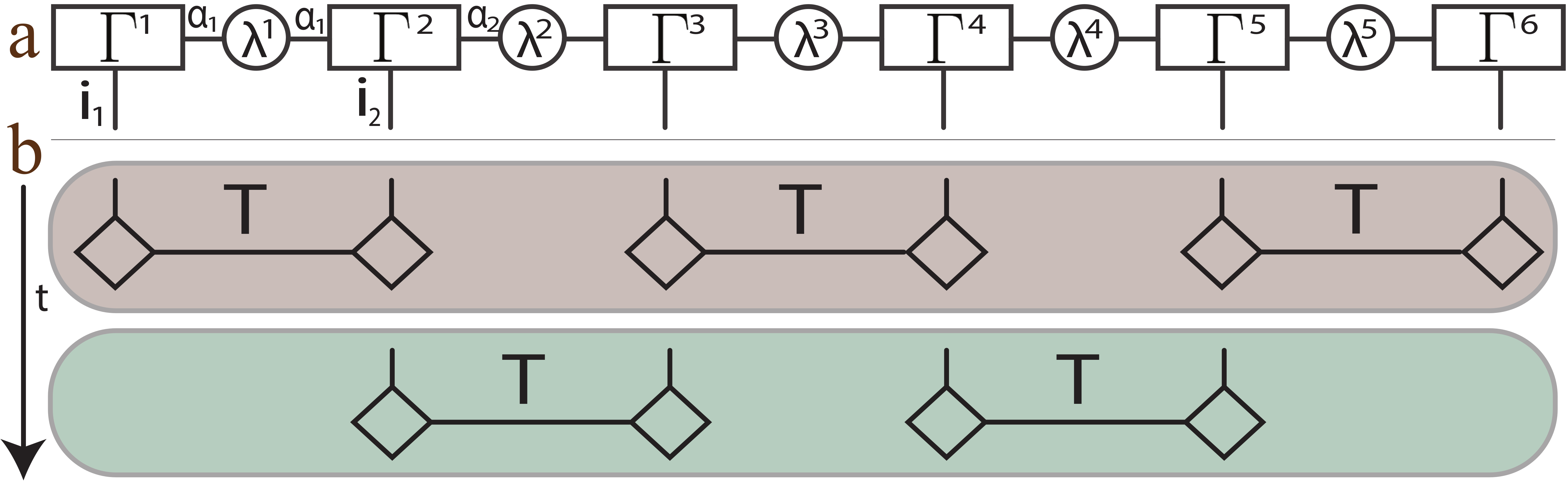
Figure 1: (a) Tensor train (matrix product state) decomposition and (b) Suzuki-Trotter propagation (see text for more details).

Operations involving multiple dimensions (indices), especially distant, destroy TT structure, so additional procedures are required to restore it. Generally, it would imply effectively the same procedure as initial decomposition. However, in this paper, we only use convolutions involving two neighboring indices. Thus, only one local reorthogonalization is required.

Consider an operation $T_{j,j+1}$:

$$A^{\prime}\left[i_{1}\ldots i_{j}i_{j+1}\ldots i_{N}\right]=\sum_{i^{\prime}_{j},i_{j}}T_{j,j+1}[i_{j},i^{\prime}_{j};i_{j+1},i^{\prime}_{j+1}]A\left[i_{1}\ldots i^{\prime}_{j}i^{\prime}_{j+1}\ldots i_{N}\right].$$ (7)

It affects a pair of the corresponding tensors,

$$\Gamma^{[j]i_{j}}_{\alpha_{j-1}\alpha_{j}},\;\lambda^{[l]}_{\alpha_{j}},\;\Gamma^{[j+1]i_{j+1}}_{\alpha_{j}\alpha_{j+1}}\rightarrow\sum_{i_{j}^{\prime}i_{j+1}^{\prime},\alpha_{j}}T_{j,j+1}[i_{j},i^{\prime}_{j};i_{j+1},i^{\prime}_{j+1}]\Gamma_{\alpha_{j-1}\alpha_{j}}^{[j]i_{j}^{\prime}}\lambda^{[l]}_{i_{j}}\Gamma^{[j+1]i_{j+1}^{\prime}}_{\alpha_{j}\alpha_{j+1}}.$$ (8)

To perform reorthogonalization, we introduce matrix $K\left[i_{j},i_{j+1};\alpha_{j-1},\alpha_{j+1}\right]$. Next we reshape indexes, perform SVD, and reshape indexes back vidal_tebd :

$$K[\alpha_{j-1},i_{j};\alpha_{j+1}i_{j+1}]=\Gamma^{\prime[j]i_{j}}_{\alpha_{j-1}\alpha_{j}}\lambda^{\prime[j]}_{\alpha_{j}}\Gamma^{\prime[j+1]i_{j+1}}_{\alpha_{j}\alpha_{j+1}}.$$ (9)

Such operation takes only $\mathcal{O}(R^{3})$ steps and this scaling does not depend on $N$. Moreover, it modifies only a pair of relevant tensors so multiple pairwise operations that act in independent subspaces may be parallelized. The TT representation allows also for fast realizations of other algebraic operations: calculation of partial or full traces, norm, scalar products, additions, etc oseled .

II.2 Tensor-Train Propagation

Algorithm 1 : TEBD method implementation

1:upload: system $\&$ method parameters (N, $T_{j}[i_{j},i^{\prime}_{j}]$, $T_{j,j+1}[i_{j},i^{\prime}_{j},i_{j+1},i^{\prime}_{j+1}]$, $dt$, $T_{\rm{max}}$, $R$), initial state ($\Gamma^{[j]i_{j}}_{\alpha_{j-1}\alpha_{j}}$, $\lambda^{[j]}_{\alpha_{j}}$)

2:for $t=0$ to $T_{\rm{max}}$ do

3:     propagate all $\Gamma^{[j]i_{j}}_{\alpha_{j-1}\alpha_{j}}$ on $[t;t+dt/2]$

4:     propagate $\Gamma^{[j]i_{j}}_{\alpha_{j-1}\alpha_{j}}$, $\lambda^{[j]}_{\alpha_{j}}$, $\Gamma^{[j+1]i_{j+1}}_{\alpha_{j}\alpha_{j+1}}$ with odd $j$ on $[t;t+dt/2]$ $\triangleright$ 4-6 do with hard cutoff of the local bond dimension

5:     propagate $\Gamma^{[j]i_{j}}_{\alpha_{j-1}\alpha_{j}}$, $\lambda^{[j]}_{\alpha_{j}}$, $\Gamma^{[j+1]i_{j+1}}_{\alpha_{j}\alpha_{j+1}}$ with even $j$ on $[t;t+dt]$

6:     propagate $\Gamma^{[j]i_{j}}_{\alpha_{j-1}\alpha_{j}}$, $\lambda^{[j]}_{\alpha_{j}}$, $\Gamma^{[j+1]i_{j+1}}_{\alpha_{j}\alpha_{j+1}}$ with odd $j$ on $[t+dt/2;t+dt]$

7:     propagate all $\Gamma^{[j]i_{j}}_{\alpha_{j-1}\alpha_{j}}$ on $[t+dt/2;t+dt]$

8:end for

9:save results

10:release memory

The TT representation provides a basis for an approximate tensor propagation algorithms. Here we use Time-Evolving Block Decimation (TEBD) scheme vidal_tebd ; ver , which was specifically designed for quantum systems but applicable also in the general case. Consider a tensor flow governed by an evolution generator consisting only of operations acting on one or two adjacent dimensions,

$$\frac{d}{dt}A[i_{1}\ldots i_{N}]=\sum_{j}\sum_{i_{j}}T^{[1]j}_{i_{j}}A[i_{1}\ldots i_{j}\ldots i_{N}]+\sum_{j_{1},j_{2}}\sum_{i_{j_{1}},i_{j_{2}}}T^{[2]j}_{i_{j_{1}},i_{j_{2}}}A[i_{1}\ldots i_{j_{1}}i_{j_{2}}\ldots i_{N}].$$ (10)

We use standard time discretization to iteratively integrate this equation (starting from some initial tensor). In terms of operations the solution reads

$$A(t+dt)=L(dt)A(t)=\\ =\exp\left[\left(\sum_{j}\hat{T}^{[1]j}+\hat{T}^{[2]j}\right)dt\right]A(t).$$ (11)

As $T$ operators generally do not commute, we have to approximate the matrix exponents. A way to minimize the error is to separate the operators into groups as large as possible such that all the operators belonging to one group commute with each other. All one-dimension operators commute by default, and two-dimension acting on odd/even pairs commute within their oddity groups; see Fig. 1b. We utilize this fact and use modified second order Suzuki-Trotter decomposition schollw :

$$L(dt)\approx L_{1}(dt/2)L_{2}^{\text{odd}}(dt/2)L_{2}^{\text{even}}(dt)L_{2}^{\text{odd}}(dt/2)L_{1}(dt/2),$$

$$L_{1}(dt)=\prod_{j=1}^{N}L^{i}_{1}(dt),\>L_{2}^{\text{even/odd}}(dt)=\prod_{j\in\{\text{even/odd}\}}L^{i}_{2}(dt),$$ (12)

$$L^{i}_{1}(dt)=e^{\hat{T}^{[1]j}dt},\;L^{i}_{2}(dt)=e^{\hat{T}^{[2]j}dt}.$$ (13)

Note that the standard approach is to adsorb one-index operators $L_{1}$ into $L_{2}$, but we find it numerically beneficial to separate them. Each factor of $L_{1}$ and $L_{2}$ can be calculated by using Eqs.  (6) and (8) respectively. Furthermore, as they commute by construction, corresponding computation can be parallelized. Each two-index operator may include a cut-off if after the reorthogonalizationm Eq. (9), the number of singular value exceeds bound dimension $R$. Corresponding accumulated truncation error is then calculated as a sum of local errors (4) over all the operation during evolution up to time $t$,

$$E(t,R)=\sum_{j=1}^{t/dt}\sum_{\{L^{i}_{2}(dt_{j})\}}E^{(j)}_{i}(R).$$ (14)

Computations are dominated by SVD, so resulting complexity is $\mathcal{O}(NR^{3})$, where $R$ is the bond dimension. With $\mathcal{O}(N)$ cores available, it becomes $\mathcal{O}(R^{3})$ and thus the computational task is perfectly scalable.

II.3 Lindblad Equation

We apply both TT and TEBD methods to evolve numerically many-body open quantum models. The state of such systems is described by a density matrix $\varrho(t)$ of the size $M^{N}\times M^{N}$, where $N$ is the number of particles/spins and $M$ is number of the local states, which we put to $M=2$ for a $1/2$-spins that we consider in the paper. Evolution of a quantum system in contact with the environment is governed by Lindblad equation book

$$\dot{\varrho}(t)=\mathcal{L}\varrho(t)=\mathcal{L}_{H}\varrho(t)+\mathcal{L}_{\mathrm{dis}}\varrho(t)=-i\left[H,\varrho(t)\right]+\sum_{s=1}^{M}\gamma_{s}\left[D_{s}\varrho(t)D^{\dagger}_{s}-\frac{1}{2}\{D^{\dagger}_{s}D_{s},\varrho(t)\}\right],$$ (15)

where $\mathcal{L}$ is the Lindblad superoperator consisting of conservative $\mathcal{L}_{H}$ and dissipative $\mathcal{L}_{\mathrm{dis}}$ parts, $H$ is Hamiltonian, $D_{s}$ are dissipation operators, and $\gamma_{s}$ are corresponding dissipation rates. There is a stationary state solution for any Lindblad superoperator $\mathcal{L}\varrho(\infty)=0$ which is unique (aside of special cases of symmetries which we do not address here).

Many-body density operator $\varrho$ can be represented as an $2N$-dimensional tensor $\varrho\left[i_{1},i_{2}\ldots i_{N};i_{1}^{\prime},i_{2}^{\prime}\ldots i_{N}^{\prime}\right]$ where every pair of indexes $i_{j},i_{j}^{\prime}$ (each one runs from $1$ to $2$) correspond to the $j$-th qubit/spin. The models we consider include only one- and two-particle interactions, which thus involve up to four indexes of $\varrho$. To overcome this, we use vectorization procedure ver and glue together indexes of each particle forming $\varrho\left[i_{1}i_{1}^{\prime};i_{2}i_{2}^{\prime}\ldots i_{N}i_{N}^{\prime}\right]$ – $N$-dimension tensor with each dimension going from $1$ to $4$. This allows applying TEBD scheme (II.2) as long as $H$ and $A_{s}$ in (15) do not couple more than two particles. However, as we restrict the accessible space to the bond dimension $R$, evolution can only start from initial MPO conditions belonging to this space. In the models considered further, we use an extreme case of product initial states, $r_{j}=1$, $\forall j$; as we aim at the stationary states, we have complete freedom when choosing initial conditions (though other choices can be more beneficial from the relaxation-speed point of view).

III Model system

As test-bed models, we use spin chains from Refs. znid ; NN . Here we only briefly described them.

Both chains consist of $N$ spins. Hamiltonian part of evolution is governed by the Heisenberg XXZ model with local disordered potential

$$H=\sum_{i}\sigma^{x}_{i}\sigma^{x}_{i+1}+\sigma^{y}_{i}\sigma^{y}_{i+1}+J\sigma^{z}_{i}\sigma^{z}_{i+1}+h_{i}\sigma^{z}_{i},$$ (16)

where $\sigma_{i}$ are Pauli matrices, $J$ is interaction strength parameter and $h_{i}$ are uncorrelated random value uniformly distributed in $[-h,h]$. Open boundary conditions are used.

In Ref. znid , a disordered spin chain with next-neighbor coupling and two “thermal reservoirs” – each one represented by pair of Lindblad operators causing excitation (relaxation) and acting on the two end spins, $i=1,N$, – were considered,

$$D_{\pm}^{i=1}=\sqrt{1\pm\mu}\sigma^{\pm}_{1},\;D_{\pm}^{i=N}=\sqrt{1\mp\mu}\sigma^{\pm}_{N},$$ (17)

where $\mu$ is bias responsible for the formation of non-equilibrium steady state with directed non-zero current. In the limit $\mu\rightarrow 0$, the stationary state is an infinite temperature ’(maximally mixed’) state, that is the normalized identity. By assuming $\mu\ll 1$, one could address the linear-response regime. The transport of the spin charge through a chain in the stationary regime was considered and the current scaling with $N$ was estimated.

The authors managed to achieve a model size of $N=400$, which is an unprecedented size for many-body open quantum models. The complexity of the computational experiments is increased by the fact that the systems needed a considerable propagation time in order to reach the stationary state (this is because the dissipation was acting at the chain ends only). Finally, to obtain scaling dependencies, averaging over disorder realizations was performed. At the same time, this work provides little detail about the resources used for numerical simulations. We considered the obtained results as a challenge and decided to reproduce them – at least for $N\simeq 100$.

As an additional test-bed, we use a model from another recent work NN . In this paper, disordered spins chains in which all spins are subjected to the action of dissipation were considered. Dissipative terms couple each pair of spins,

$$D_{l}=(\sigma_{l}^{+}+\sigma_{l+1}^{+})(\sigma_{l}^{-}-\sigma_{l+1}^{-}),$$ (18)

which try to make neighboring spins oscillating out of phase (‘anti-synchronization’). The maximal size of the models used in numerical simulations, reported in this work, was $N=32$. Among other characteristics, scaling of the so-called operational entanglement entropy  Prosen2007 was considered. We use this quantifier in our numerical experiments, in which we tried to reach $N=128$.

IV Implementation

The method described in Section II is implemented as shown in Algorithm 1. The algorithm is implemented using the C++ programming language. We found, that the matrix operations (mainly SVD) are the most time-consuming parts of the algorithm. In this regard, we employ the Armadillo software library integrated with highly optimized mathematical routines from the Intel Math Kernel Library to improve performance. Finally, Armadillo/MKL routines take about 50-80% of computation time during the propagation step depending on the current system state.

The algorithm assumes performing a set of integration operations for individual components of the system at every time step. These operations are not independent but can be ordered according to their dependencies for the organization of parallel computations. In particular, all one- and two-particle interactions can be performed completely in parallel.

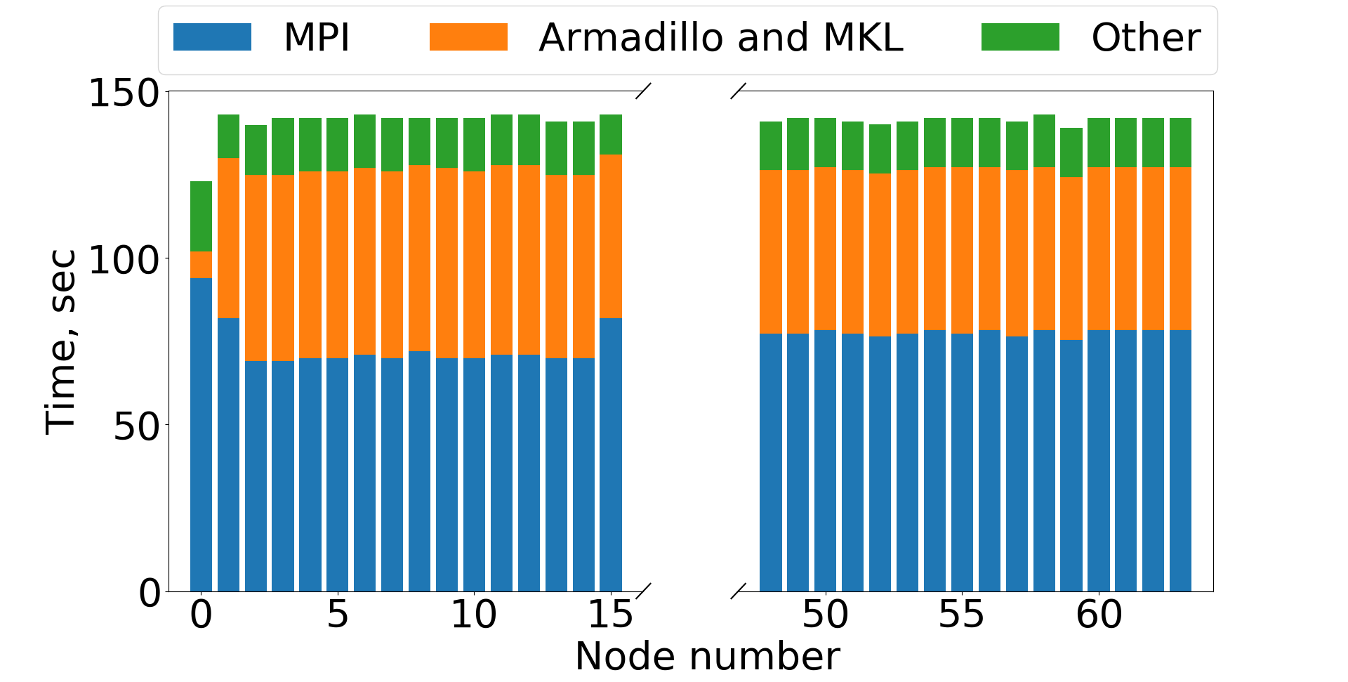
Figure 2: Distribution of computational and communication functions run time. 64 MPI-processes were executed on four nodes of the cluster.

The cluster parallelization is done by using the MPI technology. We apply the classic master-worker scheme for parallelization of the algorithm. For that, the single managing MPI-process (master) forms separate tasks for one– and two–particle interactions, monitors their dependencies from each other and readiness, distributes tasks to all other processes (workers) and accumulates the results.

All computational experiments have been done on the Lobachevsky cluster with a $2\times 8$-core Intel Xeon CPU E5-2660, 2.20GHz, 64 GB RAM, Infiniband QDR interconnect. The code was compiled with the Intel C++ Compiler, Intel Math Kernel Library and Intel MPI from the Intel Parallel Studio XE suite of development tools and the Armadillo library.

We integrate model from Ref. znid with following parameters: $N=128$, $R=50$, $T_{\rm{max}}=50$, $dt=0.1$. Parallel code was run on four computational nodes of the cluster (1 MPI-process per CPU core, 64 MPI-processes overall). Total computation time was 143 s. The resulted diagram for the distribution of computational and communication functions run time is presented in Fig. 2. It is shown that the calculations are fairly well balanced, which is an undoubted advantage of the parallelization scheme. However, MPI communications take a significant part of the computation time, while further increasing the number of cluster nodes used will not significantly speed up the calculations, which is a limitation of the scheme. Computational efficiency (ratio of computation time to total execution time) was 47%.

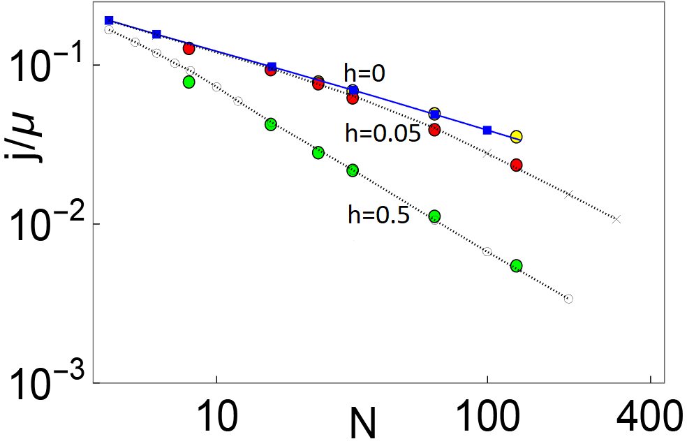
Figure 3: Scaling of the spin current $j$ through a disordered spin chain with $N$ spins for different values of disorder strength $h$. Our results (big colored circles) are plotted on top of the results (lines and other symbols) reported in Ref. znid ). The maximal size of the model system used in our simulations is $N=128$. For every set of parameters, we performed averaging over $20$ disorder realizations. The propagation time step $dt=0.1$ and bond dimension $R=50$.

V Results

We find that it is possible to reproduce - with high accuracy – the results reported in Ref. znid by using bond-dimension $R=50$. On Figure. 3 we present a comparison of the results of the sampling we perform with our code (big circles; yellow, red and green) with the results by Žnidaric̆ and his co-authors. We use propagation step $dt=0.1$ and propagate every system up to $t=10^{4}$, irrespectively of its size. It is not the most optimal way to sample (for example, it would be more effective to determine arrival of the system at the asymptotic state by monitoring the value of the spin current); however, at this stage, we tried to make the sampling procedure as simple as possible. For every value of $N$ and disorder strength $h$, we additionally performed averaging for $20$ disorder realizations. Each realization took from $2$ minutes to $2$ hours depending on the size of the system and involved up to two nodes (for large system sizes, $N>64$).

For the model from Ref. NN we study the dynamics of the operator entanglement entropy (for a fixed disorder realization) for different bond dimensions. We found that $R_{c}=360$ constitutes a threshold value after which the asymptotic entropy does not change upon further increase of the bond dimension. The calculation time for this value of bond dimension was four weeks of continuous propagation on four computing nodes.

We analyze also the evolution of accumulated error 14 in this case. It is noteworthy that saturation of the operator entropy, which signals the arrival to the asymtotic state, is not accompanied by the saturation of the error. The latter continues to grow in a power-law manner, see the dashed line in Fig. 4b. This means that MPO states – even with $R=480$ – are different from the genuine steady state of the model [which is the zero-value eigenelement of the corresponding Lindbladian (16 - 18)].

VI Conclusions

We presented a parallel implementation of the MPO-TEBD algorithm to propagate many-body open quantum systems. Parallelization is performed using the MPI technology and employs the master-worker scheme for computational tasks distribution. High-performance implementations of linear algebra from the Intel MKL were used to better utilize computational resources of modern hardware.

A series of numerical experiments was performed to determine the accuracy and limits of applicability of the developed code. In particular, the effect of the number of SVD numbers kept after each propagation step (bond-dimension $R$) on the accuracy of the method was investigated. We found that threshold value $R_{c}$ after which saturation of the relevant characteristics is observed and fuhrer increase of bond dimension does not change their values.

The performance tests on the Lobachevsky cluster demonstrated that $64$ MPI processes running on four computational nodes is the optimal configuration for the model systems with $N=128$ spins. As a next step, we plan to explore the possibility of further improvements of the parallelization by reducing the communications and increasing the efficiency of using computational resources. After that, we hope to reach the limit $N\simeq 400$ with the test-bed models.

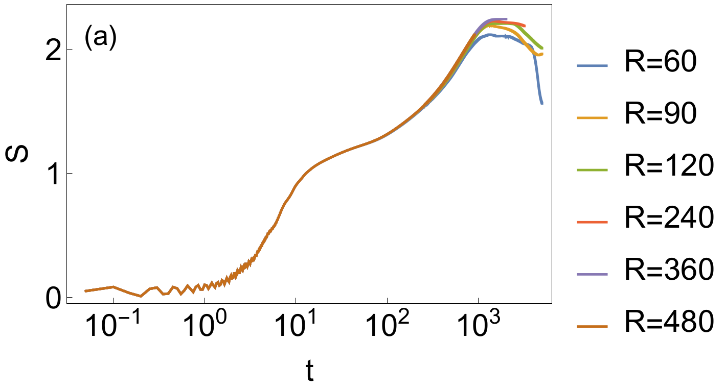
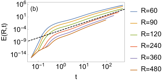
Figure 4: (a) Evolution of the operator entanglement entropy $S$ for a single disorder realization for the model from Ref. NN , for different values of bond dimension $R$. The propagation time step $dt=0.1$ and the system size is $N=128$. Note that for $R=480$ we did not reach the asymptotic ’plateau’ because it was not possible to numerically propagate system further (we hit the two-week limit). (b) Increase of the accumulated truncation error (14) in time.

VII Acknowledgments

The authors acknowledge support of the Russian Foundation for Basic Research and the Government of the Nizhni Novgorod region of the Russian Federation, grant # 18-41-520004. IV acknowledges support by the Institute for Basic Science, Project Code (IBS-R024-D1), and by the Korea University of Science and Technology Overseas Training program.

References

References

- (1) J. Eisert, M. Friesdorf, and C. Gogolin, Nature Phys. 11, 124 (2015).
- (2) J. M. Gambetta, J. M. Chow, and M. Steffen, npj Quant. Inf. 3, 2 (2017).
- (3) Breuer, H.-P., and F. Petruccione, The Theory of Open Quantum Systems (Oxford University Press, Oxford, 2002).
- (4) https://en.wikipedia.org/wiki/Titan (supercomputer)
- (5) T. G. Kolda and B. W. Bader, SIAM Rev. 51, 455 (2009).
- (6) A. Cichocki, Era of Big Data processing: a new approach via Tensor Networks and Tensor Decompositions, https://arxiv.org/abs/1403.2048.
- (7) I. V. Oseledets, SIAM J. Sci. Comput. 33, 2295 (2011).
- (8) D. Perez-Garcia, F. Verstraete, M.M. Wolf, J.I. Cirac, Quantum Inf. Comput. 7, 401 (2007); U. Schollwöck, Ann. Phys. 326, 96 (2011).
- (9) U. Schollwoeck, Ann. of Phys. 326(1) (2010).
- (10) J. Haegeman, C. Lubich, I. Oseledets, B. Vandereycken, and F. Verstraete, Phys. Rev. B 94, 165116 (2016).
- (11) G. Vidal, Phys. Rev. Lett. 91, 147902 (2003).
- (12) M. Zwolak and G. Vidal, Phys. Rev. Lett. 93, 207205 (2004).
- (13) M. Žnidaric̆, A. Scardicchio, and V. K. Varma, Phys. Rev. Lett. 117, 040601 (2016).
- (14) I. Vakulchyk, I. Yusipov, M. Ivanchenko, S. Flach, and S. Denisov, Phys. Rev. B 98, 020202(R).
- (15) G. Vidal, Phys. Rev. Lett. 91(14) (2003)
- (16) T. Prosen and I. Pižorn, Phys. Rev. A. 76, 032316 (2007).