Semidefinite relaxation of multi-marginal
optimal transport for strictly correlated electrons in second quantization

Abstract

We consider the strictly correlated electron (SCE) limit of the fermionic quantum many-body problem in the second-quantized formalism. This limit gives rise to a multi-marginal optimal transport (MMOT) problem. Here the marginal state space for our MMOT problem is the binary set $\{0,1\}$, and the number of marginals is the number $L$ of sites in the model. The costs of storing and computing the exact solution of the MMOT problem both scale exponentially with respect to $L$. We propose an efficient convex relaxation to the MMOT which can be solved by semidefinite programming (SDP). In particular, the semidefinite constraint is only of size $2L\times 2L$. We further prove that the SDP has dual attainment, in spite of the lack of Slater’s condition (i.e. the primal SDP does not have any strictly feasible point). In the context of determining the lowest energy of electrons via density functional theory, such dual attainment implies the existence of an effective potential needed to solve a nonlinear Schrödinger equation via self-consistent field iteration. We demonstrate the effectiveness of our methods on computing the ground state energy of spinless and spinful Hubbard-type models. Numerical results indicate that our SDP formulation yields comparable results when using the unrelaxed MMOT formulation. We also describe how our relaxation methods generalize to arbitrary MMOT problems with pairwise cost functions.

1 Introduction

A central yet formidable task of quantum chemistry is to determine the ground-state energy of many electrons. Although many electronic structure theories have been proposed to tackle this problem with exponential complexity in number of electrons, the Kohn-Sham density functional theory (DFT) [20, 22] remains one of the most popular techniques due to its relatively cheap cost. The Kohn-Sham DFT (KS-DFT) reduces the computational complexity by approximating the Coulombic interaction term (more precisely, the exchange-correlation term) with a functional only depending on the density of the electrons. Therefore, the success of the widely-used KS-DFT hinges on the accuracy of the approximate functionals that capture the Coulombic interactions between the particles.

In this paper, we consider solving the MMOT problem, which is related to a particular choice of the functional, the strictly correlated electron (SCE) functional $E_{\text{sce}}$ [47]. More precisely, let $\rho\in\mathbb{R}^{L}$ be a density of $L$ discrete variables normalized to $N$:

$$\rho=[\rho_{1},\ldots,\rho_{L}]^{T}\geq 0,\quad\sum_{p=1}^{L}\rho_{p}=N.$$ (1.1)

The SCE functional is defined via the MMOT problem

$$E_{\text{sce}}[\rho] := \min_{\mu\in\Pi(\rho)}\sum_{s_{1},\ldots,s_{L}\in\{0,1\}}\sum_{p,q}C_{pq}(s_{p},s_{q})\mu(s_{1},\ldots,s_{L})$$ (1.2)

where

$$\Pi(\rho)=\{\mu\ |\ \mu\geq 0,\ \sum_{s_{1},\ldots s_{L}\setminus s_{p}}\mu(s_{1},\ldots,s_{L})=\cr\rho_{p}(s_{p})\delta_{s0}(s_{p})+(1-\rho_{p}(s_{p}))\delta_{s1}(s_{p}),\ p=1,\ldots,L\},$$ (1.3)

i.e. $\mu$ has marginal densities fixed according to $\rho$. For the case considered,

$$C_{pq}(s_{p},s_{q})=\begin{cases}v_{pq}&\text{if}\ s_{p}=s_{q}=1\\ 0&\text{otherwise},\end{cases}$$ (1.4)

for specific choice of $v_{pq}$’s. Note that the dimension of the feasible space for the MMOT problem is exponential in $L$, rendering infeasible any direct approach based on the formulation of $E_{\text{sce}}[\rho]$ as a general MMOT, at least for $L$ of moderate size. The purpose of this paper is thus to propose practical algorithms to evaluate $E_{\text{sce}}$ and $\nabla_{\rho}E_{\text{sce}}[\rho]$. Although the form of $C_{pq}$ and binary state space look rather restrictive, as we shall see the proposed methods can be easily extended to deal with more general cases.

Before moving on, we want to briefly discuss the significance of considering such a functional $E_{\text{sce}}$. In DFT, although tremendous progress has been made in the construction of approximate functionals [41, 2, 24, 40], these approximations are mostly derived by fitting known results for weakly correlated systems, for examples the uniform electron gas, single atoms, small molecules, and perfect crystal systems. Such functionals often perform well when the underlying quantum systems have single-particle energy that is significantly more important than the electron-electron interaction energy. In order to extend the capability of DFT to the treatment of strongly correlated quantum systems, one recent direction of functional development considers the limit in which the electron-electron interaction energy is infinitely large compared to other components of the total energy. The resulting limit is known as the SCE limit [47, 46, 5, 30, 11, 26, 12]. The SCE limit provides an alternative route to derive exchange-correlation energy functionals. The study of Kohn-Sham DFT with SCE-based functionals is still in its infancy, but such approaches have already been used to treat strongly correlated model systems and simple chemical systems (see e.g. [37, 7, 19]).

Contribution:

Based on the recent work of the authors [21], we propose a convex relaxation approach by imposing certain necessary constraints satisfied by the 2-marginals. The relaxed problem can be solved efficiently via semidefinite programming (SDP). While the 2-marginal formulation provides a lower bound to the optimal cost of the MMOT problem, we also propose a tighter lower bound obtained via an SDP involving the 3-marginals. The computational cost for solving these relaxed problems is polynomial with respect to $L$, and, in particular, the semidefinite constraint is only enforced on a matrix of size $2L\times 2L$. Numerical results for spinless and spinful Hubbard-type systems, demonstrate that the 2-marginal and 3-marginal relaxation schemes are already quite tight, especially when compared to the modeling error due to the Kohn-Sham SCE formulation itself.

By solving the dual problems for our SDPs, we can obtain the Kantorovich dual potentials, which yield the SCE potential needed for carrying out the self-consistent field iteration (SCF) in the Kohn-Sham SCE formalism. To this end we need to show that the dual problem satisfies strong duality and moreover that the dual optimizer is actually attained. We show that a straightforward formulation of the primal SDP does not have any strictly feasible point, and hence Slater’s condition cannot be directly applied to establish strong duality (see, e.g., [4]). By a careful study of the structure of the dual problem, we prove that the strong duality and dual attainment conditions are indeed satisfied. We also explain how the SDP relaxations introduced in this paper can be applied to arbitrary MMOT problems with pairwise cost functions. We comment that the justification of the strong duality and dual attainment conditions holds in this more general setting as well.

Related work:

A system of $N$ interacting electrons in a $d$-dimensional space can be described using either the first-quantized or the second-quantized representation. In the first-quantized representation, the number of electrons $N$ is fixed, and the electronic wavefunction is an anti-symmetric function in $\bigwedge^{N}{L}^{2}(\mathbb{R}^{d};\mathbb{C}^{2})$, which is a subset of the tensor product space $\bigotimes^{N}{L}^{2}(\mathbb{R}^{d};\mathbb{C}^{2})$. Here $\mathbb{C}^{2}$ corresponds to the spin degree of freedom. In first quantization, the anti-symmetry condition needs to be treated explicitly. By contrast, in the second-quantized formalism, one chooses a basis for a subspace of ${L}^{2}(\mathbb{R}^{d};\mathbb{C}^{2})$. In practice, the basis is of some finite size $L$, corresponding to a discretized model with $L$ sites that encode both spatial and spin degrees of freedom. The electronic wavefunction is an element of the Fock space $\mathcal{F}\cong\mathbb{C}^{2^{L}}$. The Fock space contains wavefunctions of all possible electron numbers, and finding wavefunctions of the desired electron number is achieved by constraining to a subspace of the Fock space. In the second-quantized representation, the anti-symmetry constraint is in some sense baked into the Hamiltonian operator instead of the wavefunction, and this perspective often simplifies book-keeping efforts. Due to the inherent computational difficulty of studying strongly correlated systems such as high-temperature superconductors, it is often necessary to introduce simplified Hamiltonians such as in Hubbard-type models. These model problems are formulated directly in the second-quantized formalism via specification of an appropriate Hamiltonian.

To the extent of our knowledge, all existing works on SCE treat electrons in the first-quantized representation with (essentially) a real space basis. In this paper we aim at studying the SCE limit in the second-quantized setting. Note that generally Kohn-Sham-type theories in the second-quantized representation are known as ‘site occupation functional theory’ (SOFT) or ‘lattice density functional theory’ in the physics literature [45, 28, 6, 48, 8]. A crucial assumption of this paper is that the electron-electron interaction takes the form $\sum_{p,q=1}^{L}v_{pq}\hat{n}_{p}\hat{n}_{q}$, which we call the generalized Coulomb interaction. (The meaning of the symbols will be explained in Section 2.) We remark that the form of the generalized Coulomb interaction is more restrictive than the general form $\sum_{p,q,r,s=1}^{L}v_{pqrs}\hat{a}^{\dagger}_{p}\hat{a}^{\dagger}_{q}\hat{a}_{s}\hat{a}_{r}$ appearing in the quantum chemistry literature, to which our formulation does not yet apply. Assuming a generalized Coulomb interaction, we demonstrate that the corresponding SCE problem can be formulated as a multi-marginal optimal transport (MMOT) problem over classical probability measures on the binary hypercube $\{0,1\}^{L}$. The cost function in this problem is of pairwise form. Hence the objective function in the Kantorovich formulation of the MMOT can be written in terms of only the 2-marginals of the probability measure. In order to solve the MMOT problem directly, even the storage cost of the exact solution scales as $2^{L}$, and the computational cost also scales exponentially with respect to $L$. Thus a direct approach becomes impractical even when the number of sites becomes moderately large.

In the first-quantized formulation, for a fixed real-space discretization the computational cost of the direct solution of the SCE problem scales exponentially with respect to the number of electrons $N$. This curse of dimensionality is a serious obstacle for SCE-based approaches to the quantum many-body problem. Although remarkably [16, 50] show that the solution to the discretized SCE problem is sparse, finding such a sparse solution in a high dimensional space is still difficult. We note that there are exceptional cases, for example the strictly one-dimensional systems (i.e., $d=1$) and spherically symmetric systems (for any $d$) [46], for which semi-analytic solutions exist.

In [3], the Sinkhorn scaling approach is applied to an entropically regularized MMOT problem. This method requires the marginalization of a probability measure on a product space of size that is exponential in the number of electrons $N$. Thus the complexity of this method also scales exponentially with respect to $N$. Meanwhile, a method based on the Kantorovich dual of the MMOT problem was proposed in [5, 36]. However, there are exponentially many constraints in the dual problem. Furthermore, [5] assumes a Monge solution to the MMOT problem, but it is unknown whether the MMOT problem with pairwise Coulomb cost has a Monge solution for $d=2,3$. Moreover, if it exists, the Monge solution is hard to evaluate in the context of the Coulomb cost.

Another line of work that is similar in spirit to the proposed method focuses on reducing the search space of the MMOT problem to the set of $N$-representable 2-marginals in the setting of first quantization. Such a set is then relaxed to yield larger convex domains allowing for more efficient optimization. This type of method provides a lower bound to the SCE energy. In [15], the $N$-representability constraint is relaxed to a $K$-representability constraint where $K<N$, and the resulting relaxation is solved by linear programming. To further improve the approximation quality, the aforementioned work [21] of two of the authors proposes a semidefinite relaxation-based approach to the MMOT problem arising from SCE in the first-quantized setting [21]. Furthermore, by proper treatment of the 3-marginal distributions, an upper bound to the SCE energy is recovered as well. Numerical results indicate that both the lower and upper bounds are rather tight approximations to the SCE energy.

In order to use $E_{\text{SCE}}$ in the context of KS-DFT, the duality theory for the MMOT problem needs to be established. The line of work pursued in [13, 14, 17, 10] establishes the existence of dual maximizers for the repulsive MMOT problem in the first-quantized setting. As we shall see, in second quantization we only need to deal with a discrete MMOT problem where the existence of a dual maximizer is guaranteed by linear programming duality. However, the relaxation that we propose is no longer a linear program, so in this paper we must develop a duality theory for the proposed SDP.

In the second-quantized setting, our semidefinite relaxation-based approach for finding a lower bound to the SCE energy is also related to the two-particle reduced density matrix (2-RDM) theories in quantum chemistry [9, 34, 32, 33, 38]. However, the MMOT problem in SCE only requires the knowledge of the pair density instead of the entire 2-RDM. The number of constraints in our formulation is also considerably smaller than the number of constraints in 2-RDM theories, thanks to the generalized Coulomb form of the interaction.

Organization: In Section 2, we briefly describe an appropriate formulation of Kohn-Sham DFT based on the SCE functional, which is in turn defined in terms of a MMOT problem. In Section 3, we solve the MMOT problem by introducing a convex relaxation of the set of representable 2-marginals, and we prove strong duality for the relaxed problem. In Section 4, a tighter lower bound is obtained by considering a convex relaxation of the set of representable 3-marginals. In Section 5, we comment on how a general MMOT problem with pairwise cost can be solved by directly applying the methods introduced in Sections 3 and 4. We demonstrate the effectiveness of the proposed methods through numerical experiments in Section 6, and we discuss conclusions and future directions in Section 7. For completeness, the background of KS-DFT and SCE functionals is introduced in the appendices.

2 Density functional theory in second quantization

In this section, we describe how the computation of $E_{\text{sce}}[\rho]$ and $\nabla_{\rho}E_{\text{sce}}[\rho]$ arises when computing the energy of second quantized electron using KS-DFT. Readers interested in the complete details are referred to the appendix.

Let the wavefunctions of $N$ electrons be

$$\Phi=\begin{bmatrix}\varphi_{1}&\ldots&\varphi_{N}\end{bmatrix}\in\mathbb{R}^{L\times N}.$$ (2.1)

The KS-DFT states that the ground state energy of $N$ electrons can be obtained by solving a nonlinear Schrödinger equation with a particular choice of effective potential $V_{\text{eff}}[\rho]$:

$$t\varphi_{i}+\text{diag}\left(w+\nabla_{\rho}V_{\text{eff}}[\rho]\right)\varphi_{i}=\varepsilon_{i}\varphi_{i},\quad i=1,\ldots,N$$ (2.2)

$$\rho=\mathop{\operator@font diag}\nolimits(\Phi\Phi^{*}),\quad\varphi^{*}_{i}\varphi_{j}=\delta_{ij},\ \forall i,j=1,\ldots,N.$$ (2.3)

Here $t\in\mathbb{R}^{L\times L}$ is a kinetic energy operator that has the form of a graph adjacency matrix, where $t_{pq}\neq 0$ indicates possible hopping between site $p$ and $q$. The vector $w\in\mathbb{R}^{L}$ resembles an external potential on the electrons and the effective potential functional $V_{\text{eff}}[\rho]$ models the Coulombic interactions between the electrons. Although there are many choices for $V_{\text{eff}}[\rho]$, the goal of this paper is to consider the SCE limit where

$$V_{\text{eff}}[\rho]=E_{\text{sce}}[\rho].$$ (2.4)

In $E_{\text{sce}}[\rho]$, a nonzero $v_{pq}$ implies the existence of Coulombic repulsion between site $p$ and site $q$. Obtaining the derivatives $\nabla_{\rho}E_{\text{sce}}[\rho]$ amounts to solving for the dual optimizers of the MMOT via linear programming duality.

Eq. (2.2) is a nonlinear eigenvalue problem and should be solved self-consistently. The standard iterative procedure for this task works as follows:

1. For the $k$-th iterate $\rho^{(k)}$, compute $\nabla_{\rho}E_{\text{sce}}[\rho^{(k)}]$.

2. Solve for $\{\varphi_{i}^{(k+1)}\}^{L}_{i=1}$ which satisfies:

   $$t\varphi_{i}^{(k+1)}+\text{diag}\left(w+\nabla_{\rho}E_{\text{sce}}[\rho^{(k)}]\right)\varphi_{i}^{(k+1)}=\varepsilon_{i}\varphi_{i}^{(k+1)},\quad i=1,\ldots,N$$ (2.5)

   $${\varphi_{i}^{(k+1)}}^{*}\varphi^{(k+1)}_{j}=\delta_{ij},\ \forall i,j=1,\ldots,N.$$ (2.6)

   and let $\rho^{(k+1)}:=\mathrm{diag}(\Phi^{(k+1)}\Phi^{(k+1)*})$.

3. Iterate until convergence, possibly using mixing schemes [1, 42, 29] to ensure or accelerate convergence.

Once self-consistency is reached and the iterations converge to $\rho^{\star}$, the total energy can be recovered by the relation

$$E_{\text{KS-SCE}}=\sum_{k=1}^{N}\varepsilon_{k}-\nabla_{\rho}E_{\text{sce}}[\rho^{\star}]^{T}\rho^{\star}+E_{\text{sce}}[\rho^{\star}].$$ (2.7)

Readers interested in the background on how such a nonlinear eigenvalue problem arises are referred to Appendix A.

3 Convex relaxation

In this section, we discuss an SDP relaxation, $E^{\text{sdp}}_{\text{sce}}[\rho]$, to $E_{\text{sce}}[\rho]$ which has a polynomial problem size in $L$. Furthermore, we establish dual attainment for $E^{\text{sdp}}_{\text{sce}}[\rho]$ in order to show $\nabla_{\rho}E^{\text{sdp}}_{\text{sce}}[\rho]$ can indeed be obtained.

Let the 1-marginals

$$\mu^{(1)}_{p}(s_{p}):=\sum_{s_{1},\ldots,s_{L}\backslash\{s_{p}\}}\mu(s_{1},\ldots,s_{L})$$ (3.1)

satisfy

$$\mu^{(1)}_{p}(s)=(1-\rho_{p})\delta_{s0}+\rho_{p}\delta_{s1},\quad s=0,1.$$ (3.2)

We also have the 2-marginals $\mu^{(2)}_{pq}$ defined implicitly in terms of $\mu$ by marginalizing out all components other than $p,q$, i.e., by

$$\mu^{(2)}_{pq}(s_{p},s_{q}):=\sum_{s_{1},\ldots,s_{L}\backslash\{s_{p},s_{q}\}}\mu(s_{1},\ldots,s_{L}).$$ (3.3)

which is identified as the $2\times 2$ matrix

$$\mu^{(2)}_{pq}=\begin{bmatrix}\mu^{(2)}_{pq}(0,0)&\mu^{(2)}_{pq}(0,1)\\ \mu^{(2)}_{pq}(1,0)&\mu^{(2)}_{pq}(1,1)\end{bmatrix}.$$ (3.4)

Despite the fact that it is possible to formulate $E_{\text{sce}}[\rho]$ as a general MMOT problem which is a linear program over $\mu$, the pairwise cost:

$$C(s_{1},\ldots,s_{L})=\sum_{p\neq q}C_{pq}(s_{p},s_{q}).$$

allows one to write $E_{\text{sce}}[\rho]$ as

$$E_{\text{sce}}[\rho]=\inf_{\mu\in\Pi(\rho)}\sum_{p\neq q}\sum_{s_{p},s_{q}}C_{pq}(s_{p},s_{q})\mu^{(2)}_{pq}(s_{p},s_{q}),$$ (3.5)

or in matrix notation

$$E_{\text{sce}}[\rho]=\inf_{\mu\in\Pi(\rho)}\sum_{p\neq q}\text{Tr}[C_{pq}\mu^{(2)}_{pq}],$$ (3.6)

where ‘Tr’ indicates the matrix trace.

At first glance, it might seem that one may achieve a significant reduction of complexity by directly changing the optimization variable in Eq. (3.5) from $\mu$ to $\{\mu^{(2)}_{pq}\}_{p,q=1}^{L}$. However, extra constraints would then need to be enforced in order to relate the different 2-marginals; i.e., the two-marginals must be jointly representable in the sense that all of them could simultaneously be yielded from a single joint probability measure on $\{0,1\}^{L}$.

In this section, we show that a relaxation of the representability condition implicit in Eq. (3.5) allows us to formulate a tractable optimization problem in terms of the $\{\mu^{(2)}_{pq}\}_{p,q=1}^{L}$ alone. In fact, this optimization problem will be a semidefinite program (SDP).

3.1 Primal problem

We now derive certain necessary constraints satisfied by 2-marginals $\{\mu^{(2)}_{pq}\}_{p,q=1}^{L}$ that are obtained from a probability measure $\mu$ on $\{0,1\}^{L}$. In the following we adopt the notation

$$\mathbf{s}=(s_{1},\ldots,s_{L})\in\{0,1\}^{L}.$$

Then for any such $\mathbf{s}$, let $e_{\mathbf{s}}:\{0,1\}^{L}\rightarrow\mathbb{R}$ be the Dirac probability mass function on $\{0,1\}^{L}$ localized at $\mathbf{s}$, i.e.,

$$e_{\mathbf{s}}(\mathbf{s}^{\prime})=\delta_{\mathbf{s},\mathbf{s}^{\prime}}.$$

Note that we can also write $e_{\mathbf{s}}$ as an $L$-tensor, i.e., an element of $\mathbb{R}^{2\times 2\times\cdots\times 2}$, via

$$e_{\mathbf{s}}=e_{s_{1}}\otimes\cdots\otimes e_{s_{L}},$$

where we adopt the (zero-indexing) convention $e_{0}=[1,0]^{\top}$, $e_{1}=[0,1]^{\top}$.

Any probability measure on $\{0,1\}^{L}$ can be written as a convex combination of the $e_{\mathbf{s}}$ since they are the extreme points of the set of probability measures; in particular we can write a probability density $\mu\in\Pi(\rho)$ as

$$\mu=\sum_{\mathbf{s}}a_{\mathbf{s}}e_{\mathbf{s}},\ \ \text{where}\ \ \sum_{\mathbf{s}}a_{\mathbf{s}}=1,\ a_{\mathbf{s}}\geq 0.$$ (3.7)

From the definitions of the 1- and 2-marginals (3.1), (3.3), it follows that

$$\mu^{(1)}_{p}=\sum_{\mathbf{s}}a_{\mathbf{s}}\,e_{s_{p}},\quad\mu^{(2)}_{pq}=\sum_{\mathbf{s}}a_{\mathbf{s}}\,e_{s_{p}}\otimes e_{s_{q}}=\sum_{\mathbf{s}}a_{\mathbf{s}}\,e_{s_{p}}e_{s_{q}}^{\top}.$$ (3.8)

Now define

$$M=M(\{a_{\mathbf{s}}\})=\sum_{\mathbf{s}}a_{\mathbf{s}}\begin{bmatrix}e_{\mathbf{s}_{1}}\\ \vdots\\ e_{\mathbf{s}_{L}}\end{bmatrix}\begin{bmatrix}e_{\mathbf{s}_{1}}^{\top}\cdots e_{\mathbf{s}_{L}}^{\top}\end{bmatrix},$$ (3.9)

Then by Eq. (3.8), $M$ is the matrix of $2\times 2$ blocks $M_{pq}$ given by

$$M_{pq}=\begin{cases}\mathrm{\mathrm{diag}}(\mu_{p}^{(1)}),&p=q,\\ \mu_{pq}^{(2)},&p\neq q.\end{cases}$$ (3.10)

Accordingly we write $M=(M_{pq})\in\mathbb{R}^{(2L)\times(2L)}$. Then let $C=(C_{pq})\in\mathbb{R}^{(2L)\times(2L)}$ be the matrix of the $2\times 2$ blocks $C_{pq}$ defined above, which specifies the pairwise cost on each pair of marginals. Observe that the value of the objective function of Eq. (3.6) can in fact be rewritten as

$$\sum_{p\neq q}\text{Tr}[C_{pq}\mu^{(2)}_{pq}]=\text{Tr}[CM].$$

Then the MMOT problem Eq. (3.6) can be equivalently rephrased as

$$E_{\text{sce}}[\rho]\ =\ \underset{M\in\mathbb{R}^{(2L)\times(2L)},\,\{a_{\mathbf{s}}\}_{\mathbf{s}\in\{0,1\}^{L}}}{\mathrm{minimize}}\ \ \text{Tr}(CM)$$ (3.11)

subject to $$\ M=\sum_{\mathbf{s}}a_{\mathbf{s}}\begin{bmatrix}e_{\mathbf{s}_{1}}\\ \vdots\\ e_{\mathbf{s}_{L}}\end{bmatrix}\begin{bmatrix}e_{\mathbf{s}_{1}}^{\top}\cdots e_{\mathbf{s}_{L}}^{\top}\end{bmatrix},$$

$$\ M_{pp}=\mathrm{diag}(\mu_{p}^{(1)})\,\text{ for all }\,p=1,\ldots,L,$$

$$\ \sum_{\mathbf{s}}a_{\mathbf{s}}=1,\quad a_{\mathbf{s}}\geq 0\,\text{ for all }\,\mathbf{s}\in\{0,1\}^{L}.$$

Note that in our application to SCE, we have fixed

$$\mu^{(1)}_{p}=\begin{bmatrix}1-\rho_{p}\\ \rho_{p}\end{bmatrix}$$

in advance, i.e., $\mu^{(1)}_{p}$ is not an optimization variable.

At this point, our reformulation of the problem has not alleviated its exponential complexity; indeed, note that $\{a_{\mathbf{s}}\}_{\mathbf{s}\in\{0,1\}^{L}}$ is a vector of size $2^{L}$. However, the reformulation does suggest a way to reduce the complexity by accepting some approximation. In fact, we will omit $\{a_{\mathbf{s}}\}_{\mathbf{s}\in\{0,1\}^{L}}$ entirely from the optimization, retaining only $M$ as an optimization variable and enforcing several necessary constraints on $M$ that are satisfied by the solution of the exact problem.

First, note from the constraint (3.11) that $M$ is both entry-wise nonnegative (written $M\geq 0$) and positive semidefinite (written $M\succeq 0$). Second, the fact that the 1-marginals can be written in terms of the 2-marginals imposes additional local consistency constraints on $M$. Indeed, with $\mathbf{1}_{2}\in\mathbb{R}^{2}$ denoting the vector of all ones, we can write

$$\mu^{(2)}_{pq}\mathbf{1}_{2}=\mu^{(1)}_{p},\quad p\neq q,$$ (3.13)

from which it follows that

$$M_{pq}\mathbf{1}_{2}=\begin{bmatrix}1-\rho_{p}\\ \rho_{p}\end{bmatrix},\quad p,q=1,\ldots,L.$$ (3.14)

Then we obtain the relaxation

$$E_{\text{sce}}[\rho]\ \geq\ E_{\text{sce}}^{\text{sdp}}[\rho]\ :=\ \underset{M\in\mathbb{R}^{(2L)\times(2L)}}{\mathrm{minimize}}\ \ \text{Tr}(CM)$$ (3.15)

subject to $$\ M\succeq 0,$$ (3.16)

$$\ M_{pq}\geq 0\,\text{ for all }\,p,q=1,\ldots,L\ (p\neq q),$$ (3.17)

$$\ M_{pq}\mathbf{1}_{2}=\mu_{p}^{(1)}\,\text{ for all }\,p,q=1,\ldots,L\ (p\neq q),$$

$$\ M_{pp}=\mathrm{diag}(\mu_{p}^{(1)})\,\text{ for all }\,p=1,\ldots,L.$$

Again, $\mu^{(1)}_{p}$ is not an optimization variable. It is actually helpful to reformulate the primal 2-marginal SDP (3.15) as

$$\ E_{\text{sce}}^{\text{sdp}}[\rho]\ =\ \underset{M\in\mathbb{R}^{(2L)\times(2L)}}{\mathrm{minimize}}\ \ \text{Tr}(CM)$$ (3.19)

subject to $$\ M\succeq 0,$$ (3.20)

$$\ M_{pq}\geq 0\,\text{ for all }\,p,q=1,\ldots,L\ (p<q),$$ (3.21)

$$\ M_{pq}\mathbf{1}_{2}=\mu_{p}^{(1)}\,\text{ for all }\,p,q=1,\ldots,L\ (p<q),$$ (3.22)

$$\ M_{pq}^{\top}\mathbf{1}_{2}=\mu_{q}^{(1)}\,\text{ for all }\,p,q=1,\ldots,L\ (p<q),$$ (3.23)

$$\ M_{pp}=\mathrm{diag}(\mu_{p}^{(1)})\,\text{ for all }\,p=1,\ldots,L.$$ (3.24)

Note that this formulation is equivalent to (3.15), given the symmetry of $M$ (implicit in the notation $M\succeq 0$). However, the new formulation removes a few redundant constraints and will help us derive a more intuitive dual problem. The problem (3.19) will be referred to as the primal 2-marginal SDP, or the primal problem for short. Note that the optimal value of the primal problem is in fact attained because the constraints (3.20)-(3.24) define a compact feasible set.

Reflecting back on the derivation, we caution that replacing $E_{\text{sce}}[\rho]$ with $E_{\text{sce}}^{\text{sdp}}[\rho]$ comes at a price. Since we only enforce certain necessary conditions on $M$, the 2-marginals that we recover from $M$ may not in fact be the 2-marginals of a joint probability measure on $\{0,1\}^{L}$. Thus $E_{\text{sce}}^{\text{sdp}}[\rho]$ should in general only be expected to be a lower-bound to $E_{\text{sce}}[\rho]$, though we will see that the error is often small in practice.

3.2 Dual problem

As detailed in Section 2, in order to implement the SCF for Kohn-Sham SCE it is necessary to compute $\nabla_{\rho}E_{\text{sce}}[\rho]$. After replacing the density functional $E_{\text{sce}}[\rho]$ with the efficient approximation $E_{\text{sce}}^{\text{sdp}}[\rho]$, the same derivation motivates us to compute $\nabla_{\rho}E_{\text{sce}}^{\text{sdp}}[\rho]$. This quantity can obtained by examining the convex duality of our primal 2-marginal SDP.

We let $Y\succeq 0$ be the variable dual to the constraint (3.20), $Z_{pq}\geq 0$ be dual to (3.21), $\phi_{pq}$ be dual to (3.22), $\psi_{pq}$ be dual to (3.23), and finally let $X_{p}$ be dual to (3.24). Note that $Z_{pq}\in\mathbb{R}^{2\times 2}$ and $\phi_{pq},\psi_{pq}\in\mathbb{R}^{2}$ for each $p<q$, and $X_{p}\in\mathbb{R}^{2\times 2}$ for each $p$.

Then our formal Lagrangian is of the form

$$\mathcal{L}\left(M,Y,\{Z_{pq},\phi_{pq},\psi_{pq}\}_{p<q},\{X_{p}\}\right),$$

where the domains of $M$ is the set of symmetric $2L\times 2L$ matrices (equivalently, it is convenient to think of $M$ as depending only on its upper-block-triangular part), and the dual variables are as specified above (i.e., only $Y\succeq 0$ and $Z_{pq}\geq 0$ are constrained), and more specifically we have (omitting the arguments of $\mathcal{L}$ from the notation)

$$\mathcal{L} = \text{Tr}(CM)-\text{Tr}(YM)$$

$$\ \ -\ 2\sum_{p<q}\left[\text{Tr}(Z_{pq}^{\top}M_{pq})+\phi_{pq}^{\top}\left(M_{pq}\mathbf{1}_{2}-\mu^{(1)}_{p}\right)+\psi_{pq}^{\top}\left(M_{pq}^{\top}\mathbf{1}_{2}-\mu^{(1)}_{q}\right)\right]$$

$$\ \ -\ \sum_{p}\text{Tr}\left(X_{p}^{\top}\left[M_{pp}-\mathrm{diag}(\mu_{p}^{(1)})\right]\right).$$

It is helpful to realize the identities

$$\phi_{pq}^{\top}M_{pq}\mathbf{1}_{2}=\text{Tr}\left(M_{pq}[\mathbf{1}_{2}\phi_{pq}^{\top}]\right),\quad\psi_{pq}^{\top}M_{pq}^{\top}\mathbf{1}_{2}=\text{Tr}\left(M_{pq}[\psi_{pq}\mathbf{1}_{2}^{\top}]\right).$$

Then, recognizing that $C=C^{\top}$ and $Y=Y^{\top}$ (so that $C_{pq}^{\top}=C_{qp}$ and $Y_{pq}^{\top}=Y_{qp}$), minimization over $M$ of the Lagrangian (3.2) yields the dual problem

$$\underset{Y,\,\{Z_{pq},\phi_{pq},\psi_{pq}\}_{p<q},\,\{X_{p}\}}{\mathrm{maximize}}\ \ \sum_{p}\text{Tr}\left(X_{p}^{\top}\,\mathrm{diag}(\mu_{p}^{(1)})\right)+2\sum_{p<q}\left(\phi_{pq}^{\top}\mu_{p}^{(1)}+\psi_{pq}^{\top}\mu_{q}^{(1)}\right)$$ (3.27)

subject to $$\ Y\succeq 0,$$

$$\ Z_{pq}\geq 0\,\text{ for }\,p<q,$$

$$\ C_{pq}-Y_{pq}-Z_{pq}-\phi_{pq}\mathbf{1}_{2}^{\top}-\mathbf{1}_{2}\psi_{pq}^{\top}=0\,\text{ for }\,p<q,$$ (3.28)

$$\ C_{pp}-Y_{pp}-X_{p}^{\top}=0.$$ (3.29)

Observe that the variables $Z_{pq}$ can be removed by combining constraints (3.27) and (3.28) to yield

$$C_{pq}-Y_{pq}-\phi_{pq}\mathbf{1}_{2}^{\top}-\mathbf{1}_{2}\psi_{pq}^{\top}\geq 0.$$

Moreover, $X_{p}$ can be removed simply by substituting $X_{p}=-Y_{pp}$ into the objective function (recall that $C_{pp}=0$). These reductions yield

$$\underset{Y,\,\{\phi_{pq},\psi_{pq}\}_{p<q}}{\mathrm{maximize}}\ \ 2\sum_{p<q}\left(\phi_{pq}\cdot\mu_{p}^{(1)}+\psi_{pq}\cdot\mu_{q}^{(1)}\right)-\sum_{p,s}Y_{pp}(s,s)\mu_{p}^{(1)}(s)$$ (3.30)

subject to $$\ Y\succeq 0,$$ (3.31)

$$\ \phi_{pq}\mathbf{1}_{2}^{\top}+\mathbf{1}_{2}\psi_{pq}^{\top}\leq C_{pq}-Y_{pq}\,\text{ for }\,p<q.$$ (3.32)

Here we think of $Y_{pp}(s,s)$ as the $(s,s)$ entry of the $2\times 2$ matrix $Y_{pp}$, and likewise $\mu_{p}^{(1)}(s)$ is the $s$-th entry of $\mu_{p}^{(1)}$.

The dual problem may be interpreted as follows. Observe that for $Y$ fixed (e.g., fixed to its optimal value), the maximization problem decouples into a set of independent maximization problems for each pair of marginals. We think of $\widetilde{C}_{pq}:=C_{pq}-Y_{pq}$ as defining an effective cost function for each pair of marginals. Then the decoupled problem for a pair $p<q$ is exactly the Kantorovich dual problem in standard (i.e., not multi-marginal) optimal transport, specified by cost function $\widetilde{C}_{pq}$ and marginals $\mu_{p}^{(1)}$, $\mu_{q}^{(1)}$ [49]. In other words, after fixing $Y$, our problem decouples into independent standard optimal transport problems for each pair of marginals. Nonetheless, these problems are in turn themselves coupled via the optimization over $Y\succeq 0$.

Recall that we wanted to compute $\nabla_{\rho}E_{\text{sce}}^{\text{sdp}}[\rho]$. Assuming that strong duality holds, as shall be established later, the optimal value of the dual problem (3.30) is in fact equal to $E_{\text{sce}}^{\text{sdp}}[\rho]$. (Recall that here we think of the 1-marginals $\mu_{p}^{(1)}=[1-\rho_{p},\rho_{p}]^{\top}$ as being defined in terms of $\rho$.) Hence we can compute derivatives by evaluating the gradient of the objective function (3.30) with respect to $\rho$ at the optimizer $\left(Y,\,\{\phi_{pq},\psi_{pq}\}_{p\neq q}\right)$. (If the optimizer is not unique, then in general we will get a subgradient [44].)

To carry out this program, first note that $\frac{\partial}{\partial\rho_{r}}\mu_{p}^{(1)}=\delta_{pr}[-1,1]^{\top}$. Therefore the partial derivative of the objective function (3.30) with respect to $\rho_{r}$ yields

$$\frac{\partial E_{\text{sce}}^{\text{sdp}}[\rho]}{\partial\rho_{r}}=2\sum_{q>r}[\phi_{rq}(1)-\phi_{rq}(0)]+2\sum_{p<r}[\psi_{pr}(1)-\psi_{pr}(0)]-[Y_{rr}(1,1)-Y_{rr}(0,0)].$$

If one extends the definition of $\phi_{pq},\psi_{pq}$ to $p>q$ via the stipulation $\phi_{pq}=\psi_{qp}$, then one has

$$\frac{\partial E_{\text{sce}}^{\text{sdp}}[\rho]}{\partial\rho_{r}}=\sum_{p\neq r}[\phi_{rp}(1)-\phi_{rp}(0)]-[Y_{rr}(1,1)-Y_{rr}(0,0)].$$

3.3 Strong duality and dual attainment

In this subsection, we show that the optimizer of the dual problem  (3.30) can be attained. Before embarking on a proof of dual attainment, we note that Sion’s minimax theorem [23] guarantees that the duality gap is zero as the domain of the primal problem is compact, as stated in the following Lemma.

Lemma 1.

The primal and dual problems (3.19) and (3.30), respectively, have the same (finite) optimal value.

However, in order to compute the SCE potential, we actually require not only that the duality gap is zero, but also that the supremum in the dual problem is attained. One might hope to verify Slater’s condition [4], which provides a standard method for verifying both strong duality and such ‘dual attainment’ simultaneously. The trouble is that Slater’s condition requires the existence of a feasible interior point $M$, i.e., a point $M$ satisfying $M\succ 0$ and $M_{pq}>0$ for all $p\neq q$. This scenario is in fact impossible since for example the vector

$$\begin{bmatrix}\mathbf{1}_{2}^{\top}&-\mathbf{1}_{2}^{\top}&0&\cdots&0\end{bmatrix}^{\top}\in\mathbb{R}^{2L}$$ (3.33)

lies in the null space of any feasible $M$, hence $M\succ 0$ never holds for feasible $M$.

Instead of using Slater’s condition, we will prove dual attainment via a very careful study of the structure of the dual problem.

Theorem 2.

The optimal value of the dual 2-marginal SDP (3.30) is attained. By Lemma 1, this optimal value is equal to the optimal value of the primal 2-marginal SDP (3.19).

Proof.

Without loss of generality we assume

$$0<\rho_{p}<1,\quad p=1,\ldots,L.$$ (3.34)

To see why this assumption can be made, observe that if $\rho_{p}\in\{0,1\}$ for some $p$, then attainment for the dual problem (3.30) can be reduced to attainment for a strictly smaller dual 2-marginal SDP. We leave further details of such a reduction to the reader.) Also, for later reference, we let $F(Y,\{\phi_{pq},\psi_{pq}\}_{p<q})$ denote the objective function (3.30), and we let $\mathcal{D}$ denote the feasible domain defined by the constraints (3.31), (3.32).

Now to get started, observe that if we fix $Y\succeq 0$ and view (3.30) as an optimization problem over $\{\phi_{pq},\psi_{pq}\}_{p<q}$ only, the resulting problem is in fact a linear program. Let us call this the $Y$-program, more specifically:

$$\underset{\{\phi_{pq},\psi_{pq}\}_{p<q}}{\mathrm{maximize}}\ \ 2\sum_{p<q}\left(\phi_{pq}\cdot\mu_{p}^{(1)}+\psi_{pq}\cdot\mu_{q}^{(1)}\right)-\sum_{p,s}Y_{pp}(s,s)\mu_{p}^{(1)}(s)$$

subject to $$\ \phi_{pq}\mathbf{1}_{2}^{\top}+\mathbf{1}_{2}\psi_{pq}^{\top}\leq C_{pq}-Y_{pq}\,\text{ for }\,p<q.$$

In fact we may consider the $Y$-program for any matrix $Y$, and this will slightly simplify some discussion later. Observe that each $Y$-program is feasible, and the optimal values $f(Y)$ of all $Y$-programs are finite. Since they are linear programs, this means that the optimal values of the $Y$-programs can be attained. Thus for each $Y$, there exist $\phi_{pq}^{\star}(Y)$, $\psi_{pq}^{\star}(Y)$ for $p<q$ which optimize the $Y$-program, i.e., attain the value $f(Y)$. By construction $f(Y)$ is concave, hence continuous, in $Y$.

Now let $d_{0}=f(0)$, so $d^{\star}\geq d_{0}$, where $d^{\star}$ is the optimal value of the dual problem (3.30). Hence the feasible set of (3.30) could be refined to $S\cap\mathcal{D}$, where

$$S:=\{Y\succeq 0\,:\,f(Y)\geq d_{0}\},$$

without altering the optimal value. Now if $S$ were compact, then the lemma would follow. To see this, note that since $d^{\star}<\infty$ (which follows from weak duality), we could take an optimizing sequence $(Y^{(k)},\{\phi_{pq}^{(k)},\psi_{pq}^{(k)}\}_{p<q})$ for (3.30), where $Y^{(k)}\in S\cap\mathcal{D}$. Then by compactness we could find a subsequence of $Y^{(k)}$ converging to some $Y^{\star}$. By the continuity of $f$, then $f(Y^{\star})=d^{\star}$. Then it would follow that the optimum is attained at the point $(Y^{\star},\{\phi_{pq}^{\star}(Y^{\star}),\psi_{pq}^{\star}(Y^{\star})\}_{p<q})$.

Unfortunately, $S$ is not compact, but we will find a further constraint that does yield a compact feasible set without altering the optimal value. Then the preceding argument will complete the proof.

To further constrain the feasible set, we will observe a transformation of $Y$ that preserves the value of $f(Y)$, then ‘mod out’ by this transformation. To this end, first note that via the discussion of Kantorovich duality following (3.30) we can in fact write

$$f(Y)=-\sum_{p=1}^{L}\text{Tr}\left[Y_{pp}\mathrm{diag}(\mu_{p}^{(1)})\right]+\sum_{p,q=1}^{L}\mathbf{OT}_{pq}(C_{pq}-Y_{pq}),$$

where $\mathbf{OT}_{pq}(A)$ is the optimal cost of the standard optimal transport problem with cost matrix $A$ and marginals $\mu_{p}^{(1)},\mu_{q}^{(1)}$.

Then let $P\in\mathbb{R}^{(2L)\times(L-1)}$ be defined by

$$P:=\begin{bmatrix}\mathbf{1}_{2}&&&\\ -\mathbf{1}_{2}&\mathbf{1}_{2}&&\\ &-\mathbf{1}_{2}&\ddots&\\ &&\ddots&\mathbf{1}_{2}\\ &&&-\mathbf{1}_{2}\end{bmatrix},$$ (3.35)

and let its columns be denoted $P_{i}$ for $i=1,\ldots,L-1$. Then we claim that

$$f(Y)=f\left(Y+P_{i}v^{\top}+vP_{i}^{\top}\right)$$ (3.36)

for any $Y$, $v\in\mathbb{R}^{2L}$, and any $i=1,\ldots,L-1$. To prove this, write

$$v=\left[v_{1}^{\top}\cdots v_{L}^{\top}\right]^{\top},$$

where $v_{q}\in\mathbb{R}^{2}$ for $q=1,\ldots,L$. Then observe that, via the discussion of Kantorovich duality following the statement (3.30) of the dual problem, we can in fact write

$$f(Y)=-\sum_{p=1}^{L}\text{Tr}\left[Y_{pp}\mathrm{diag}(\mu_{p}^{(1)})\right]+2\sum_{p<q}\mathbf{OT}_{pq}(C_{pq}-Y_{pq}),$$

where $\mathbf{OT}_{pq}(A)$ is the optimal cost of the standard optimal transport problem with cost matrix $A$ and marginals $\mu_{p}^{(1)},\mu_{q}^{(1)}$.

Then compute

$$f(Y+P_{i}v^{\top}) = -\sum_{p=1}^{L}\text{Tr}\left[Y_{pp}\mathrm{diag}(\mu_{p}^{(1)})\right]-\text{Tr}\left[\mathbf{1}_{2}v_{i}^{\top}\mathrm{diag}(\mu_{i}^{(1)})\right]+\text{Tr}\left[\mathbf{1}_{2}v_{i+1}^{\top}\mathrm{diag}(\mu_{i+1}^{(1)})\right]$$

$$\ \ +\ 2\sum_{p<q,\,p\notin\{i,i+1\}}\mathbf{OT}_{pq}(C_{pq}-Y_{pq})$$

$$\ \ +\ 2\sum_{q=i+1}^{L}\mathbf{OT}_{iq}(C_{iq}-Y_{iq}-\mathbf{1}_{2}v_{q}^{\top})+2\sum_{q=i+2}^{L}\mathbf{OT}_{i+1,q}(C_{i+1,q}-Y_{i+1,q}+\mathbf{1}_{2}v_{q}^{\top}).$$

Now

$$\text{Tr}\left[\mathbf{1}_{2}v_{i}^{\top}\mathrm{diag}(\mu_{i}^{(1)})\right]=v_{i}\cdot\mu_{i}^{(1)},\quad\text{Tr}\left[\mathbf{1}_{2}v_{i+1}^{\top}\mathrm{diag}(\mu_{i+1}^{(1)})\right]=v_{i+1}\cdot\mu_{i+1}^{(1)},$$

and moreover it is not hard to see that

$$\mathbf{OT}_{pq}(A+\mathbf{1}_{2}x^{\top})=\mathbf{OT}_{pq}(A)+x\cdot\mu_{q}^{(1)}$$

for any $A\in\mathbb{R}^{2\times 2},x\in\mathbb{R}^{2}$, hence

$$f(Y+P_{i}v^{\top}) = -\sum_{p=1}^{L}\text{Tr}\left[Y_{pp}\mathrm{diag}(\mu_{p}^{(1)})\right]-v_{i}\cdot\mu_{i}^{(1)}+v_{i+1}\cdot\mu_{i+1}^{(1)}+2\sum_{p<q}\mathbf{OT}_{pq}(C_{pq}-Y_{pq})$$

$$\ \ -\ 2\sum_{q=i+1}^{L}v_{q}\cdot\mu_{q}^{(1)}+2\sum_{q=i+2}^{L}v_{q}\cdot\mu_{q}^{(1)}$$

$$= f(Y)-v_{i}\cdot\mu_{i}^{(1)}-v_{i+1}\cdot\mu_{i+1}^{(1)}.$$

Similarly

$$f(Y+vP_{i}^{\top}) = -\sum_{p=1}^{L}\text{Tr}\left[Y_{pp}\mathrm{diag}(\mu_{p}^{(1)})\right]-\text{Tr}\left[v_{i}\mathbf{1}_{2}^{\top}\mathrm{diag}(\mu_{i}^{(1)})\right]+\text{Tr}\left[v_{i+1}\mathbf{1}_{2}^{\top}\mathrm{diag}(\mu_{i+1}^{(1)})\right]$$

$$\ \ +\ 2\sum_{p<q,\,q\notin\{i,i+1\}}\mathbf{OT}_{pq}(C_{pq}-Y_{pq})$$

$$\ \ +\ 2\sum_{p=1}^{i-1}\mathbf{OT}_{pi}(C_{pi}-Y_{pi}-v_{p}\mathbf{1}_{2}^{\top})+2\sum_{p=1}^{i}\mathbf{OT}_{p,i+1}(C_{p,i+1}-Y_{p,i+1}+v_{p}\mathbf{1}_{2}^{\top})$$

$$= f(Y)+v_{i}\cdot\mu_{i}^{(1)}+v_{i+1}\cdot\mu_{i+1}^{(1)}.$$

Since the identities

$$f(Y+P_{i}v^{\top})=f(Y)-v_{i}\cdot\mu_{i}^{(1)}-v_{i+1}\cdot\mu_{i+1}^{(1)},\quad f(Y+vP_{i}^{\top})=f(Y)+v_{i}\cdot\mu_{i}^{(1)}+v_{i+1}\cdot\mu_{i+1}^{(1)}$$

hold for arbitrary $Y$, the claim Eq. (3.36) is proven.

Then from Eq. (3.36) it follows that

$$f(Y)=f(Y+PB+B^{\top}P^{\top})$$ (3.37)

for arbitrary $B\in\mathbb{R}^{(L-1)\times(2L)}$.

Now let $Q\in\mathbb{R}^{(2L)\times(L+1)}$ be defined by

$$Q=\begin{bmatrix}w_{1}&0&\cdots&0&w_{2}\\ 0&w_{1}&&\vdots&\vdots\\ \vdots&&\ddots&&\\ 0&\cdots&&w_{1}&w_{2}\end{bmatrix},\quad w_{1}=\frac{1}{2}\begin{bmatrix}1\\ -1\end{bmatrix},\quad w_{2}=\frac{1}{2}\mathbf{1}_{2},$$

and observe that $Q$ is chosen so that each column of $Q$ is orthogonal to each column of $P$. Moreover $P$ and $Q$ both have full rank, so it follows that $R:=[Q,P]$ is invertible.

Then for fixed $Y$, consider

$$\hat{Y}=R^{\top}YR=\left(\begin{array}[]{cc}Q^{\top}YQ&Q^{\top}YP\\ P^{\top}YQ&P^{\top}YP\end{array}\right).$$

We aim to choose $B$ such that

$$R^{\top}(PB+B^{\top}P^{\top})R=\left(\begin{array}[]{cc}0&0\\ P^{\top}PBQ&P^{\top}PBP\end{array}\right)+\left(\begin{array}[]{cc}0&Q^{\top}B^{\top}P^{\top}P\\ 0&P^{\top}B^{\top}P^{\top}P\end{array}\right)$$

cancels $\hat{Y}$ on all but the top-left block. Using $Q^{\top}P=0$ (and $P^{\top}Q=0$), one can readily check that such a choice is given by

$$-B=(P^{\top}P)^{-1}\hat{Y}_{21}(Q^{\top}Q)^{-1}Q^{\top}+\frac{1}{2}(P^{\top}P)^{-1}\hat{Y}_{22}(P^{\top}P)^{-1}P^{\top}.$$

By the identity (3.37), it follows that we can further restrict the feasible set by intersecting with

$$S^{\prime}=\left\{Y\,:\,R^{\top}YR=\left(\begin{array}[]{cc}*&0\\ 0&0\end{array}\right)\succeq 0,\ f(Y)\geq d_{0}\right\}.$$ (3.38)

In fact $S^{\prime}$ is compact, and the proof is complete pending the proof of this claim, to which we now turn.

Observe that for $(Y,\{\phi_{pq},\psi_{pq}\}_{p<q})$ feasible, we may multiply Eq. (3.32) from the left by $\big{(}\mu_{p}^{(1)}\big{)}^{\top}$ and from the right by $\mu_{q}^{(1)}$ to obtain

$$\phi_{pq}\cdot\mu_{p}^{(1)}+\psi_{pq}\cdot\mu_{q}^{(1)} \leq \big{(}\mu_{p}^{(1)}\big{)}^{\top}[C_{pq}-Y_{pq}]\big{(}\mu_{q}^{(1)}\big{)}$$

$$= \big{(}\mu_{q}^{(1)}\big{)}^{\top}[C_{pq}-Y_{pq}]^{\top}\big{(}\mu_{p}^{(1)}\big{)}$$

$$= \text{Tr}\left([C_{pq}-Y_{pq}]^{\top}\big{(}\mu_{p}^{(1)}\big{)}\big{(}\mu_{q}^{(1)}\big{)}^{\top}\right).$$

By substituting this inequality into the objective function $F(Y,\{\phi_{pq},\psi_{pq}\}_{p<q})$ as defined in (3.30), we see that

$$F(Y,\{\phi_{pq},\psi_{pq}\}_{p<q})\leq\text{Tr}(CM)-\text{Tr}(YM).$$

for $(Y,\{\phi_{pq},\psi_{pq}\}_{p<q})$ feasible, where

$$M_{pq}:=\begin{cases}\mathrm{\mathrm{diag}}\big{(}\mu_{p}^{(1)}\big{)},&p=q\\ \big{(}\mu_{p}^{(1)}\big{)}\big{(}\mu_{q}^{(1)}\big{)}^{\top},&p\neq q.\end{cases}$$

It follows then that

$$f(Y)\leq\text{Tr}(CM)-\text{Tr}(YM).$$

In fact $M$ can be written $M=Q\widetilde{M}Q^{\top}$, where $\widetilde{M}\succ 0$. This can be verified directly by taking

$$\widetilde{M}=\begin{bmatrix}\widetilde{\rho}_{1}\\ \vdots\\ \widetilde{\rho}_{L}\\ 1\end{bmatrix}\begin{bmatrix}\widetilde{\rho}_{1}&\cdots&\widetilde{\rho}_{L}&1\end{bmatrix}+\text{diag}\left(\begin{bmatrix}1-\widetilde{\rho}_{1}^{2}&\cdots&1-\widetilde{\rho}_{L}^{2}&0\end{bmatrix}\right),$$

with

$$\widetilde{\rho}_{p}=1-2\rho_{p},\quad p=1,\ldots,L.$$

Note that $\widetilde{M}\succ 0$ by the assumption (3.34). Hence

$$f(Y)\leq\text{Tr}(CM)-\text{Tr}(Q^{\top}YQ\widetilde{M}).$$

Now since $\widetilde{M}\succ 0$, there exists a scalar $K>0$ such that if $Y\succeq 0$ and $Q^{\top}YQ\not\preceq K$, then $f(Y)<d_{0}$. But $Q^{\top}YQ$ is the upper-left block of $R^{\top}YR$, so it follows from the definition (3.38) of $S^{\prime}$ that that

$$S^{\prime}\subset\left\{Y\,:\,R^{\top}YR=\left(\begin{array}[]{cc}A&0\\ 0&0\end{array}\right),\,0\preceq A\preceq K\right\},$$

from which it follows that $S^{\prime}$ is compact, and the proof is complete. ∎

Remark 3.

Note that the proof of Theorem 2 guarantees that the domain of the dual problem (3.30) can be restricted to $Y$ of the form $Y=Q\widetilde{Y}Q^{\top}$, yielding a ‘reduced’ dual problem in which $\widetilde{Y}$ replaces $Y$ as an optimization variable. In fact, one can also verify directly that any $M$ feasible for the primal problem (3.19) satisfies $MP=0$, hence the domain of the primal problem can be restricted to $M$ of the form $M=Q\widetilde{M}Q^{\top}$, likewise yielding a reduced primal problem.

But despite this apparent symmetry, the latter observation need not imply the former in a more general SDP setting, and the arguments given in the proof of Theorem 2, which use more of the specific structure of our problem, do appear to be necessary to the proof of dual attainment for this problem.

Moreover, observe with caution that the dual of such a reduced primal problem is not the reduced dual problem!

4 Tighter lower bound via 3-marginals

In this section, we further tighten the convex relaxation proposed in Section 3 with a formulation that additionally involves the 3-marginals.

One defines the 3-marginals $\mu^{(3)}_{pqr}$ (for $p,q,r,$ distinct) induced by a probability measure $\mu$ on $\{0,1\}^{L}$ via

$$\mu^{(3)}_{pqr}(s_{p},s_{q},s_{r}):=\sum_{s_{1},\ldots,s_{L}\backslash\{s_{p},s_{q},s_{r}\}}\mu(s_{1},\ldots,s_{L}).$$ (4.1)

There is no 3-marginal analog known to us of the semidefinite constraint that can be enforced using the 2-marginals. However, we can nonetheless use the 3-marginals to enforce additional necessary local consistency constraints. Indeed, the 2-marginals can themselves be written in terms of the 3-marginals via

$$\mu^{(2)}_{pq}(s_{p},s_{q})=\sum_{s_{r}}\mu^{(3)}_{pqr}(s_{p},s_{q},s_{r}).$$ (4.2)

Accordingly, we will include $K=\{K_{pqr}\}$ for distinct $p,q,r$ as optimization variables for the 3-marginals. Note that based on Eq. (4.1) we can enforce that $K$ is symmetric, by which we mean that

$$K_{pqr}(s_{p},s_{q},s_{r})=K_{\sigma(p)\sigma(q)\sigma(r)}(s_{\sigma(p)},s_{\sigma(q)},s_{\sigma(r)})$$

for any permutation $\sigma$ on the letters $\{p,q,r\}$. If we were to extend $K_{pqr}$ by zeros to $p,q,r$ not distinct, then we could think of $K\in\mathbb{R}^{(2L)\times(2L)\times(2L)}$ as a symmetric 3-tensor, with $(p,q,r)$-th $2\times 2\times 2$ block given by $K_{pqr}$. In principle the imposition of symmetry removes some redundancy in the specification of $K$.

Then we arrive at the following 3-marginal SDP:

$$\underset{M\in\mathbb{R}^{(2L)\times(2L)},\,K\in\mathbb{R}^{(2L)\times(2L)\times(2L)}}{\mathrm{minimize}}\ \ \text{Tr}(CM)$$ (4.3)

subject to $$\ M\succeq 0,$$ (4.4)

$$\ M_{pq}\geq 0\,\text{ for }p\neq q,$$ (4.5)

$$\ M_{pq}\mathbf{1}_{2}=\mu_{p}^{(1)}\,\text{ for }p\neq q,$$

$$\ M_{pp}=\mathrm{diag}(\mu_{p}^{(1)})\,\text{ for all }\,p,$$

$$\ K\geq 0,\ K\text{ symmetric},$$

$$\ M_{pq}(s_{p},s_{q})=\sum_{s_{r}}K_{pqr}(s_{p},s_{q},s_{r})\,\text{ for }p,q,r\,\text{distinct}.$$

Note that the blocks $K_{pqr}$ for $p,q,r$ not distinct are superfluous and can be discarded in an efficient optimization.

For simplicity, we omit discussion of the duality of (4.3). Since only linear constraints have been added, most of the interesting features from the mathematical viewpoint have already been discussed above. Indeed, as in Section 3.2, we may derive the dual of the 3-marginal problem (4.3), and we may certify as in Section 3.3 that the 3-marginal problem satisfies strong duality and dual attainment.

5 General MMOT with pairwise cost

As has been suggested both explicitly and via the notation, almost all of our discussion of relaxation methods for MMOT can be applied to general MMOT problems with pairwise cost functions. The main caveat is that specific references to the fact that the 1-marginal state space has two elements should be suitably generalized. For clarity, we now recapitulate our methods for the general MMOT problem with pairwise cost. The reader interested in general MMOT should still see the earlier sections for derivations, discussions, and proofs. Here we only summarize the methods.

We will consider a problem with $L$ marginals, written $\mu_{p}^{(1)}$ for $p=1,\ldots,L$. These quantities are fixed in advance and never varied in the following discussion. We let $N_{p}$ be the size of the state space of the $p$-th marginal, so $\mu_{p}^{(1)}$ is a probability vector of length $N_{p}$. Note that the marginals need not all have the same state space, i.e., $N_{p}$ can depend on $p$. We write the $p$-th state space as $\mathcal{X}_{p}:=\{1,\ldots,N_{p}\}$. Then the joint state space is given by $\mathcal{X}:=\prod_{p=1}^{L}\mathcal{X}_{p}$, and we write $\mathrm{Pr}_{p}$ for the $p$-th projection $\mathcal{X}\rightarrow\mathcal{X}_{p}$. Suppose that we are given a pairwise cost function $C_{pq}\in\mathbb{R}^{N_{p}\times N_{q}}$ for each pair $p\neq q$ of marginals. (Without loss of generality we assume $C_{pp}=0$.) Then we consider the problem

$$\min_{\mu\in\mathcal{P}(\mathcal{X})}\sum_{(s_{1},\ldots,s_{L})\in\mathcal{X}}\sum_{p,q=1}^{L}C_{pq}(s_{p},s_{q})\mu(s_{1},\ldots,s_{L}),\quad\text{s.t.}\ \ (\mathrm{Pr}_{p})\#\mu=\mu_{p}^{(1)},\ p=1,\ldots,L.$$ (5.1)

Here $\mu:\mathcal{X}\rightarrow\mathbb{R}$ can be thought of as an $L$-tensor whose $p$-th index ranges from $1,\ldots,N_{p}$. Again, the objective function of such a MMOT problem can be rephrased in terms of the 2-marginals:

$$\min_{\mu\in\mathcal{P}(\mathcal{X})}\sum_{p\neq q}^{L}\text{Tr}(C_{pq}\mu^{(2)}_{pq}),\quad\text{s.t.}\ \ (\mathrm{Pr}_{p})\#\mu=\mu_{p}^{(1)},\ p=1,\ldots,L,$$ (5.2)

where the 2-marginals $\mu^{(2)}_{pq}$ are here implicitly defined in terms of the optimization variable $\mu$.

Then we introduce the 2-marginal primal SDP

$$\underset{M\in\mathbb{R}^{N_{\mathrm{tot}}\times N_{\mathrm{tot}}}}{\mathrm{minimize}}\ \ \text{Tr}(CM)$$ (5.3)

subject to $$\ M\succeq 0,$$ (5.4)

$$\ M_{pq}\geq 0\,\text{ for all }\,p,q=1,\ldots,L\ (p\neq q),$$ (5.5)

$$\ M_{pq}\mathbf{1}_{N_{q}}=\mu_{p}^{(1)}\,\text{ for all }\,p,q=1,\ldots,L\ (p\neq q),$$

$$\ M_{pp}=\mathrm{diag}(\mu_{p}^{(1)})\,\text{ for all }\,p=1,\ldots,L.$$

Here $N_{\mathrm{tot}}:=\sum_{p=1}^{L}N_{p}$ and $\mathbf{1}_{k}$ denotes the vector of ones of length $k$. The dual of (5.3) is given by

$$\underset{Y,\,\{\phi_{pq},\psi_{pq}\}_{p<q}}{\mathrm{maximize}}\ \ 2\sum_{p<q}\left(\phi_{pq}\cdot\mu_{p}^{(1)}+\psi_{pq}\cdot\mu_{q}^{(1)}\right)-\sum_{p,s}Y_{pp}(s,s)\mu_{p}^{(1)}(s)$$

subject to $$\ Y\succeq 0,$$

$$\ \phi_{pq}\mathbf{1}_{N_{q}}^{\top}+\mathbf{1}_{N_{p}}\psi_{pq}^{\top}\leq C_{pq}-Y_{pq}\,\text{ for }\,p<q.$$

In (5) is it understood that $Y\in\mathbb{R}^{N_{\mathrm{tot}}\times N_{\mathrm{tot}}}$ and moreover $\phi_{pq}\in\mathbb{R}^{N_{p}}$, $\psi_{pq}\in\mathbb{R}^{N_{q}}$.

By generalizing the discussion of Theorem 2, we have strong duality for the 2-marginal SDP, hence the optimal values of (5.3) and (5) are equal, and moreover the dual problem admits a maximizer. (The primal problem admits a maximizer trivially because the feasible set is compact.)

Finally, we turn to the 3-marginal primal SDP

$$\underset{M\in\mathbb{R}^{N_{\mathrm{tot}}\times N_{\mathrm{tot}}},\,K\in\mathbb{R}^{N_{\mathrm{tot}}\times N_{\mathrm{tot}}\times N_{\mathrm{tot}}}}{\mathrm{minimize}}\ \ \text{Tr}(CM)$$ (5.8)

subject to $$\ M\succeq 0,$$ (5.9)

$$\ M_{pq}\geq 0\,\text{ for }p\neq q,$$ (5.10)

$$\ M_{pq}\mathbf{1}_{N_{q}}=\mu_{p}^{(1)}\,\text{ for }p\neq q,$$

$$\ M_{pp}=\mathrm{diag}(\mu_{p}^{(1)})\,\text{ for all }\,p,$$

$$\ K\geq 0,\ K\text{ symmetric},$$

$$\ M_{pq}(s_{p},s_{q})=\sum_{s_{r}}K_{pqr}(s_{p},s_{q},s_{r})\,\text{ for }p,q,r\,\text{distinct}.$$

For simplicity we omit the concrete formulation of the corresponding dual problem, but we note that strong duality and dual attainment can be proved by methods similar to those applied in the 2-marginal case.

6 Numerical results

In this section, we numerically demonstrate the effectiveness of the proposed methods on solving for the ground state energy of Hubbard-type models. The Hubbard model is a prototypical model for strongly-correlated quantum systems, and is considered to be of significant importance to model behaviors such as high temperature superconductivity [43]. To investigate the numerical performance of the SDP formulation, we consider one-dimensional spinless Hubbard models and two-dimensional spinful Hubbard models.

6.1 One-dimensional spinless model

Here we consider a 1D spinless Hubbard-like model defined by the Hamiltonian of Eq. (A.6), in which we take

$$t_{pq}=\begin{cases}1&\text{if }|q-p|=1,\\ 0&\text{otherwise}\end{cases}$$ (6.1)

and consider two different cases of $v$, with next-nearest neighbor (NN) interaction,

$$v_{pq}=\begin{cases}U/2&\text{if }|q-p|=1,\\ U/40&\text{if }|q-p|=2,\\ 0&\text{otherwise}\end{cases}$$ (6.2)

and next-next-nearest neighbor interaction (NNNN)

$$v_{pq}=\begin{cases}U/2&\text{if }|q-p|=1,\\ U/20&\text{if }|q-p|=2,\\ U/200&\text{if }|q-p|=3,\\ 0&\text{otherwise.}\end{cases}$$ (6.3)

The reason why we omit the obvious scenario of the nearest neighbor (NN) interaction is that in such a case, we find that our convex relaxation becomes numerically exact and hence we consider the case to be not representative. We do not have a proof yet to explain why our convex relaxation scheme can be numerically exact.

We will compare the Kohn-Sham SCE energies yielded by our methods with one another, as well as with the exact ground-state energy (A.7), which is computed via exact diagonalization (ED) in the OpenFermion [35] software package. The MMOT problems arising in Kohn-Sham SCE and their SDP relaxations are solved in MATLAB with the CVX software package [18].

We refer to the exact self-consistent Kohn-Sham SCE solution obtained by solving the original linear programming (LP) problem for MMOT as the ‘LP’ solution. Hence the tightness of the Kohn-Sham SCE lower bound (A.15) itself can be evaluated by comparing the exact energy with the LP energy, while the tightness of our SDP relaxations of the relevant MMOT problems (which, in turn, yield lower bounds for the Kohn-Sham SCE energy) can be evaluated by comparing the LP energy with the 2- and 3-marginal SDP energies. We refer to these two sources of error, respectively, as the ‘Kohn-Sham SCE model error’ and the ‘error due to relaxation.’

In Figs. 6.1(a) and 6.2(a), we plot $E/U$ with respect to $U$ for $v$ as in Eqs. (6.2) and (6.3), respectively. In these experiments, $L=14$ and $N=9$. The energy differences of the Kohn-Sham SCE solutions from the exact energy are plotted in Figs. 6.1(b) and 6.2(b). It is confirmed numerically that the LP energy lower-bounds the exact energy, and in turn the SDP energies lower-bound the LP energy. While the 3-marginal SDP lower bound is noticeably tighter than the 2-marginal SDP lower bound, the error due to relaxation is dominated by the Kohn-Sham SCE model error in both cases.

Since the effective potential is of interest in Kohn-Sham DFT, in Fig. 6.3 we plot the SCE potential (A.16) at self-consistency in the case of $v$ as in Eq. (6.3). It can be seen that the 3-marginal SDP performs better than the 2-marginal SDP in this regard, as one might expect. (However, note carefully that although it is guaranteed a priori that the 3-marginal SDP provides a lower bound on the energy that is at least as tight as that of the 2-marginal SDP, no such comparison is theoretically guaranteed in advance for the effective potential.)

To study the scaling of energy in the thermodynamic limit $L\rightarrow\infty$, in Fig 6.4(a), we plot $E/U$ as a function of $L$ by fixing $U=5$ and a filling factor of $N/L=2/3$. In Fig 6.4(b), we plot the total runtime of our methods on a MacBook Pro with a 2.3GHz Core I5 CPU and 16GB of memory.

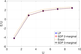
(a)

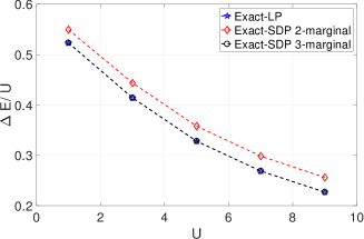
(b)

Fig. 6.1: Spinless 1D fermionic lattice model with $v$ as in Eq. (6.2), $L=14$, $N=9$. (a) $E/U$ as a function of $U$. (b) Difference between the exact energy and the Kohn-Sham SCE energies obtained from the unrelaxed LP and the SDP relaxations.

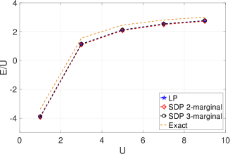
(a)

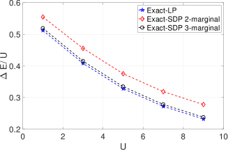
(b)

Fig. 6.2: Spinless 1D fermionic lattice model with $v$ as in Eq. (6.3), $L=14$, $N=9$. (a) $E/U$ as a function of $U$. (b) Difference between the exact energy and the Kohn-Sham SCE energies obtained from the unrelaxed LP and the SDP relaxations.

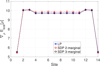
Fig. 6.3: The effective potential for the spinless 1D fermionic lattice model with $v$ as in Eq. (6.3), $U=5$, $L=14$, $N=9$. The relative $\ell^{2}$ errors for the 2- and 3-marginal formulations (compared to the unrelaxed LP formulation) are $1.2\times 10^{-2}$ and $2.7\times 10^{-3}$, respectively.

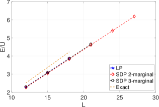
(a)

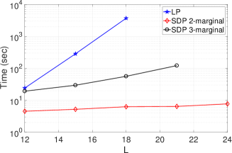
(b)

Fig. 6.4: Spinless 1D fermionic lattice model with $v$ as in Eq. (6.3), $U=5$, $N/L=2/3$. (a) $E/U$ as a function of $L$. (b) Running time as a function of $L$.

6.2 Two-dimensional spinful model

We consider a 2D generalized Hubbard type model defined by the Hamiltonian

$$\begin{split}\hat{H}=&-\sum_{i,j=1}^{L-1}\sum_{\sigma\in\{\uparrow,\downarrow\}}\left(\hat{a}_{i+1,j;\sigma}^{\dagger}\hat{a}_{i,j;\sigma}+\hat{a}_{i,j+1;\sigma}^{\dagger}\hat{a}_{i,j;\sigma}+\text{h.c.}\right)\\ &+U\sum_{i,j=1}^{L}\hat{n}_{i,j;\uparrow}\hat{n}_{i,j;\downarrow}+V\sum_{i,j=1}^{L-1}\left(\hat{n}_{i+1,j}\hat{n}_{i,j}+\hat{n}_{i,j+1}\hat{n}_{i,j}\right).\end{split}$$ (6.4)

Here $\hat{n}_{i,j}:=\hat{n}_{i,j;\uparrow}+\hat{n}_{i,j;\downarrow}$. As discussed in section 2, although the creation and annihilation operators in Eq. (6.4) involve two spatial indices and one spin index, one may of course order the operators with a single index by defining

$$b_{(j-1)L+i}=a_{i,j;\uparrow},\quad b_{(j-1)L+i+L^{2}}=a_{i,j;\downarrow}.$$

The new creation operators are fixed as the Hermitian adjoints of these new annihilation operators. The term associated with $U$ is the on-site electron-electron interaction, while $V$ specifies the nearest-neighbor electron-electron interaction. In the standard Hubbard model, we have $V=0$. (However, in the case $V=0$, the MMOT problem arising in the SCE framework becomes a trivial problem, since the interaction terms associated with different sites are decoupled.) Fig. 6.5 shows the energies for the generalized Hubbard model on a $3\times 3$ lattice, with $V=0.05\,U$ and $U$ ranging from $1.0$ to $19.0$. The number $N$ of electrons is set to be $12$. Here energies are obtained from the exact solution, the exact Kohn-Sham SCE solution obtained by linear programming (LP), and the approximate Kohn-Sham SCE solution obtained via the 2-marginal SDP relaxation. We find that the Kohn-Sham SCE formulation becomes asymptotically accurate when $U$ becomes large. Furthermore, the error due to relaxation is much smaller than the Kohn-Sham SCE model error. Fig. 6.5(b) further shows that the energy difference between the LP and 2-marginal SDP solutions is approximately constant with respect to the on-site interaction strength $U$.

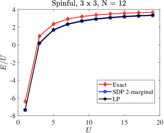
(a)

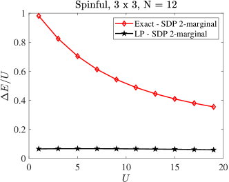
(b)

Fig. 6.5: Spinful $3\times 3$ Hubbard model with $N=12$.

7 Conclusion

In this paper, we have considered the strictly correlated electron (SCE) limit of a fermionic quantum many-body system in the second-quantized formalism. To the extent of our knowledge, the setup of the SCE problem in this setting has not appeared in the literature. Mathematically, the SCE limit requires the solution of a multi-marginal optimal transport problem over certain classical probability measures. We propose a relaxation that enforces constraints on the 2-marginals of these measures, and the relaxed problem can be solved efficiently via semi-definite programming (SDP). We prove that the SDP problem satisfies strong duality and moreover that the dual solution is attained, despite the fact that the primal problem does not possess a strictly feasible point. We consider a tighter relaxation involving the 3-marginals and discuss how our methods can be applied to completely general multi-marginal optimal transport problems with pairwise costs.

The relaxed formulation is not exact and provides only a lower bound to the SCE energy. Hence it is meaningful to compare the error due to relaxation with the Kohn-Sham SCE model error, i.e., the disparity between the Kohn-Sham SCE energy and the exact energy of the solution to the quantum many-body problem. Our numerical results for various fermionic lattice model problems indicate that the former can be much smaller than the latter, hence our convex relaxation scheme can be considered to be effective. On the other hand, as indicated in, e.g., [31], Kohn-Sham SCE is only the zero-th order approximation to the quantum many-body ground state energy in the limit of large interaction. Hence the SCE functional and SCE potential should be considered more properly as an “ingredient” for designing more accurate exchange-correlation functionals. From such a perspective, just as the exact formulation of SCE is only a model, it may even be appropriate to consider the relaxed SCE formulation as a model itself. It can capture certain strong correlation effects and can be solved efficiently.

One immediate extension of the current work is to include finite-temperature effects via entropic regularization. In fact, entropic regularization may be relevant for another reason as well. During our numerical studies, we observed that the self-consistent iteration for Kohn-Sham SCE (not the convex optimization problem solved within each iteration) can be difficult to converge. The convergence behavior may depend sensitively on the filling factor, the lattice size, and the form of the interaction. Such difficulty can arise for both the exact SCE formulation solved via linear programming and the relaxed formulations solved by SDP. Preliminary results show that entropic regularization can help make the loop easier to converge. We are not aware of any reports of such issues in the literature, and we plan to study such behavior more systematically in future work.

Appendix A Background of KS-DFT

Our goal is to compute the ground-state energy of a fermionic system with $L$ sites where each site has two states. With some abuse of terminology, we will refer to fermions simply as electrons. Also for simplicity we use a single index for all of the states, as opposed to using separate site and spin indices in the case of spinful systems. Double indexing for spinful fermionic systems can be recovered simply by rearranging indices, e.g., by associating odd state indices with spin-up components and even state indices with spin-down components.

In the second-quantized formulation, the state space is called the Fock space, denoted by $\mathcal{F}$. The occupation number basis set for the Fock space is

$$\{\ket{s_{1},\ldots,s_{L}}\}_{s_{i}\in\{0,1\},i=1,\ldots,L},$$

which is an orthonormal basis set satisfying

$$\braket{s_{i_{1}},\ldots,s_{i_{L}}}{s_{j_{1}},\ldots,s_{j_{L}}}=\delta_{i_{1}j_{1}}\cdots\delta_{i_{L}j_{L}}.$$ (A.1)

A state $\ket{\psi}\in\mathcal{F}$ will be written as a linear combination of occupation number basis elements as follows:

$$\ket{\psi}=\sum_{s_{1},\ldots,s_{L}\in\{0,1\}}\psi(s_{1},\ldots,s_{L})\ket{s_{1},\ldots,s_{L}},\quad\psi(s_{1},\ldots,s_{L})\in\mathbb{C}.$$ (A.2)

Hence the state vector $\ket{\psi}$ can be identified with a vector $\psi\in\mathbb{C}^{2^{L}}$, and $\mathcal{F}$ is isomorphic to $\mathbb{C}^{2^{L}}$. We call $\ket{\psi}$ normalized if the following condition is satisfied:

$$\braket{\psi}{\psi}=\sum_{s_{1},\ldots,s_{L}\in\{0,1\}}|\psi(s_{1},\ldots,s_{L})|^{2}=1.$$ (A.3)

We also refer to $\ket{0}=\ket{0,\ldots,0}$ as the vacuum state.

The fermionic creation and annihilation operators are respectively defined as

$$\begin{split}\hat{a}_{p}^{\dagger}\ket{s_{1},\ldots,s_{L}}&=(-1)^{\sum_{q=1}^{p-1}s_{q}}(1-s_{p})\ket{s_{1},\ldots,1-s_{p},\ldots,s_{L}},\\ \hat{a}_{p}\ket{s_{1},\ldots,s_{L}}&=(-1)^{\sum_{q=1}^{p-1}s_{q}}s_{p}\ket{s_{1},\ldots,1-s_{p},\ldots,s_{L}},\quad p=1,\ldots,L.\end{split}$$ (A.4)

The number operator defined as $\hat{n}_{p}:=\hat{a}^{\dagger}_{p}\hat{a}_{p}$ satisfies

$$\hat{n}_{p}\ket{s_{1},\ldots,s_{L}}=s_{p}\ket{s_{1},\ldots,s_{L}},\quad p=1,\ldots,L.$$ (A.5)

The Hamiltonian operator is assumed to take the following form:

$$\hat{H}=\sum_{p,q=1}^{L}t_{pq}\hat{a}_{p}^{\dagger}\hat{a}_{q}+\sum_{p=1}^{L}w_{p}\hat{n}_{p}+\sum_{p,q=1}^{L}v_{pq}\hat{n}_{p}\hat{n}_{q}.$$ (A.6)

Here $t\in\mathbb{C}^{L\times L}$ is a Hermitian matrix, which is often interpreted as the ‘hopping’ term arising from the kinetic energy contribution to the Hamiltonian. $w$ is an on-site term, which can be viewed as an external potential. $v\in\mathbb{C}^{L\times L}$ is also a Hermitian matrix, which may be viewed as representing the electron-electron Coulomb interaction. Note that $\hat{n}_{p}=\hat{a}_{p}^{\dagger}\hat{a}_{p}=\hat{n}_{p}\hat{n}_{p}$, hence without loss of generality we can assume the diagonal entries $t_{pp}=v_{pp}=0$ by absorbing, if necessary, such contributions into the on-site potential $w$. Following the spirit of Kohn-Sham DFT, one could think of $t,v$ as fixed matrices, and of the external potential $w$ as a contribution that may change depending on the system (in the context of DFT, $w$ represents the electron-nuclei interaction and is therefore ‘external’ to the electrons). We remark that the restriction of the form of the two-body interaction $\sum_{p,q=1}^{L}v_{pq}\hat{n}_{p}\hat{n}_{q}$ is crucial for the purpose of this paper. In particular, we do not consider the more general form $\sum_{p,q,r,s=1}^{L}v_{pqrs}\hat{a}^{\dagger}_{p}\hat{a}^{\dagger}_{q}\hat{a}_{s}\hat{a}_{r}$ as is done in the quantum chemistry literature when a general basis set (such as the Gaussian basis set) is used to discretize a quantum many-body Hamiltonian in the continuous space. In the discussion below, for simplicity we will omit the index range of our sums as long as the meaning is clear.

The exact ground state energy $E_{0}$ can be obtained by the following minimization problem:

$$E_{0}=\inf_{\ket{\psi}\in\mathcal{F}\,:\,\braket{\psi}{\psi}=1}\bra{\psi}\hat{H}-\mu\hat{N}\ket{\psi}.$$ (A.7)

Here the minimizer $\ket{\psi}$ is the many-body ground state wavefunction, and $\hat{N}:=\sum_{p}\hat{n}_{p}$ is the total number operator. $\mu$, which is called the chemical potential, is a Lagrange multiplier chosen so that the ground state wavefunction $|\psi\rangle$ has a number of electrons equal to a pre-specified integer $N\in\{0,1,\ldots,L\}$, i.e., such that

$$\braket{\psi}{\hat{N}}{\psi}=N.$$ (A.8)

It is clear that $\mu\hat{N}$ is an on-site potential, and without loss of generality we absorb $\mu$ into $w$, and hence write $\hat{H}-\mu\hat{N}$ as $\hat{H}$ in the discussion below.

The electron density $\rho\in\mathbb{R}^{L}$ is defined as

$$\rho_{p}=\braket{\psi}{\hat{n}_{p}}{\psi}=\sum_{s_{1},\ldots,s_{L}}\lvert\psi(s_{1},\ldots,s_{L})\rvert^{2}s_{p},\quad p=1,\ldots,L,$$ (A.9)

which satisfies $\sum_{p}\rho_{p}=N$. Note that

$$\bra{\psi}\sum_{p}w_{p}\hat{n}_{p}\ket{\psi}=\sum_{p}w_{p}\rho_{p}=:W[\rho].$$ (A.10)

Then we follow the Levy-Lieb constrained minimization approach [25, 27] and rewrite the ground state minimization problem (A.7) as follows:

$$\begin{split}E_{0}=&\inf_{\rho\in\mathcal{J}_{N}}\left\{\sum_{p}\rho_{p}w_{p}+\left(\inf_{\ket{\psi}\mapsto\rho,\ket{\psi}\in\mathcal{F}}\bra{\psi}\sum_{pq}t_{pq}\hat{a}_{p}^{\dagger}\hat{a}_{q}+\sum_{pq}v_{pq}\hat{n}_{p}\hat{n}_{q}\ket{\psi}\right)\right\}\\ =&\inf_{\rho\in\mathcal{J}_{N}}\{W[\rho]+F_{\text{LL}}[\rho]\},\end{split}$$ (A.11)

where

$$F_{\text{LL}}[\rho]:=\inf_{\ket{\psi}\mapsto\rho,\ket{\psi}\in\mathcal{F}}\bra{\psi}\sum_{pq}t_{pq}\hat{a}_{p}^{\dagger}\hat{a}_{q}+\sum_{pq}v_{pq}\hat{n}_{p}\hat{n}_{q}\ket{\psi}.$$ (A.12)

Here the notation $\psi\mapsto\rho$ indicates that the corresponding infimum is taken over states $\ket{\psi}$ that yield the density $\rho$ in the sense of Eq. (A.9), and the domain $\mathcal{J}_{N}$ of $\rho$ is defined by

$$\mathcal{J}_{N}:=\left\{\rho\in\mathbb{R}^{L}\ \left|\ \rho\geq 0,\,\sum_{p}\rho_{p}=N\right.\right\}.$$ (A.13)

Note that the external potential $w$ is only coupled with $\rho$ and is singled out in the constrained minimization. It is easy to see that for any $\rho\in\mathcal{J}_{N}$, the set $\{\ket{\psi}\in\mathcal{F}\,:\,\ket{\psi}\mapsto\rho\}$ is non-empty, as we may simply choose

$$\ket{\psi}=\sum_{p}\sqrt{\rho_{p}}\ket{s^{(p)}_{1},\ldots,s^{(p)}_{L}},\quad s^{(p)}_{q}=\delta_{pq}.$$

Therefore the constrained minimization problem (A.11) is in fact defined over a nonempty set for all $\rho\in\mathcal{J}_{N}$.

The functional $F_{\text{LL}}[\rho]$, which is called the Levy-Lieb functional, is a universal functional in the sense that it depends only on the hopping term $t$ and the interaction term $v$, hence in particular is independent of the potential $w$. Once the functional $F_{\text{LL}}[\rho]$ is known, $E_{0}$ can be obtained by minimization with respect to a single vector $\rho$ using standard optimization algorithms, or via the self-consistent field (SCF) iteration to be detailed below. The construction above is called the ‘site occupation functional theory’ (SOFT) or ‘lattice density functional theory’ in the physics literature [45, 28, 6, 48, 8]. To our knowledge, SOFT or lattice DFT often imposes an additional sparsity pattern on the $v$ matrix for the electron-electron interaction, so that the Hamiltonian becomes a Hubbard-type model.

A.1 Strictly correlated electron limit

Using the fact that the infimum of a sum is greater than the sum of infimums, we can lower-bound the ground state energy in the following way:

$$F_{\text{LL}}[\rho]\geq\inf_{\ket{\psi}\mapsto\rho}\bra{\psi}\sum_{pq}t_{pq}\hat{a}_{p}^{\dagger}\hat{a}_{q}\ket{\psi}+\inf_{\ket{\psi}\mapsto\rho}\bra{\psi}\sum_{pq}v_{pq}\hat{n}_{p}\hat{n}_{q}\ket{\psi}=:T[\rho]+E_{\text{sce}}[\rho],$$ (A.14)

where the functionals $T[\rho]$ and $E_{\text{sce}}[\rho]$ are defined via the last equality in the manner suggested by the notation. The first of these quantities is called the kinetic energy, and the second the strictly correlated electron (SCE) energy. The SCE approximation is obtained by treating $T[\rho]+E_{\text{sce}}[\rho]$ as an approximation for the Levy-Lieb functional. Though in general it is only a lower-bound for the Levy-Lieb functional, this bound is expected to become tight in the limit of infinitely strong interaction. We do not prove this fact in this paper (though we demonstrate it numerically below), but we nonetheless refer to this approximation as the SCE limit by analogy to the literature on SCE in first quantization [47, 46].

Due to the inequality in Eq. (A.14), we have in general the following lower bound for the total energy, which we shall call the Kohn-Sham SCE energy:

$$E_{0}\geq E_{\textrm{KS-SCE}}:=\inf_{\rho\in\mathcal{J}_{N}}\left\{W[\rho]+T[\rho]+E_{\text{sce}}[\rho]\right\}.$$ (A.15)

The advantage of the preceding manipulations is that now each term in this infimum can be computed. Specifically, $W[\rho]$ is trivial to compute, $T[\rho]$ is defined in terms of a non-interacting many-body problem (i.e., a problem with Hamiltonian only quadratic in the creation and annihilation operators), for which an exact solution can be obtained via the diagonalization of $t$ [39]. Finally, as we shall see below the SCE term (and its gradient) can be computed in terms of a MMOT problem (and its dual). Thus in principle, it would be possible to take gradient descent approach for computing the infimum in the definition (A.15) of $E_{\textrm{KS-SCE}}$.

A.1.1 The Kohn-Sham SCE equations

In practice, to compute the Kohn-Sham SCE energy we will instead adopt the self-consistent field (SCF) iteration as is common practice in Kohn-Sham DFT. It can be readily checked that $E_{\text{sce}}[\rho]$ is convex with respect to $\rho$. By the convexity of $W[\rho]$, $T[\rho]$, and $E_{\text{sce}}[\rho]$, the expression in Eq. (A.15) admits a minimizer, which is unique unless the functional fails to be strictly convex. We assume that the solution is unique and $E_{\text{sce}}[\rho]$ is differentiable for simplicity, and we derive nonlinear fixed-point equations satisfied by the minimizer as follows.

For suitable $\rho$, define the SCE potential via

$$v_{\text{sce}}[\rho]=\nabla_{\rho}E_{\text{sce}}[\rho].$$ (A.16)

Now assume that the (unique) infimum in Eq. (A.15) is obtained at $\rho^{\star}$, which is then in particular a critical point of the expression

$$W[\rho]+T[\rho]+E_{\text{sce}}[\rho].$$ (A.17)

But then $\rho^{\star}$ is also a critical point of the expression obtained by replacing $E_{\text{sce}}[\rho]$ with its expansion up to first order about $\rho^{\star}$, which is (modulo a constant term that does not affect criticality)

$$G[\rho]:=W[\rho]+T[\rho]+v_{\text{sce}}[\rho^{\star}]\cdot\rho=T[\rho]+(w+v_{\text{sce}}[\rho^{\star}])\cdot\rho.$$ (A.18)

Hence $\cdot$ means the inner product, and we are motivated to try to minimize $G[\rho]$ over $\rho\in\mathcal{J}_{N}$. But we can write

$$G[\rho]=\inf_{\ket{\psi}\mapsto\rho}\bra{\psi}\sum_{pq}h_{pq}[\rho^{\star}]\hat{a}_{p}^{\dagger}\hat{a}_{q}\ket{\psi},$$

where

$$h[\rho]:=t+\mathrm{diag}(w+v_{\text{sce}}[\rho]).$$

Here $\mathrm{diag}(\cdot)$ is a diagonal matrix. Then

$$\inf_{\rho\in\mathcal{J}_{N}}G[\rho]=\inf_{\ket{\psi}\in\mathcal{F}\,:\,\langle\psi|\psi\rangle=1,\,\langle\psi|\hat{N}|\psi\rangle=N}\bra{\psi}\sum_{pq}h_{pq}[\rho^{\star}]\hat{a}_{p}^{\dagger}\hat{a}_{q}\ket{\psi}.$$

The latter infimum is a ground-state problem for a non-interacting Hamiltonian and is obtained [39] at a so-called Slater determinant of the form

$$\ket{\psi}=\hat{c}^{\dagger}_{1}\cdots\hat{c}^{\dagger}_{N}\ket{0}.$$ (A.19)

Here the $c_{k}^{\dagger}$ are ‘canonically transformed’ creation operators defined by

$$\hat{c}^{\dagger}_{k}=\sum_{p}\hat{a}^{\dagger}_{p}\varphi_{pk},$$ (A.20)

where $\Phi=[\varphi_{1}\cdots\varphi_{N}]=[\varphi_{pk}]\in\mathbb{C}^{L\times N}$ is a matrix whose columns are the $N$ lowest eigenvectors of $h[\rho^{\star}]$. We assume the eigenvectors form an orthonormal set, i.e. $\Phi^{*}\Phi=I_{N}$.

Moreover, one may directly compute that the electron density of $|\psi\rangle$ as defined in Eq. (A.19) is given by

$$\rho_{p}=\braket{\psi}{\hat{n}_{p}}{\psi}=\sum_{k=1}^{N}\lvert\varphi_{pk}\rvert^{2},$$ (A.21)

i.e., $\rho=\mathrm{diag}(\Phi\Phi^{*})$. Hence the optimizer $\rho^{\star}$ of Eq. (A.15) solves the Kohn-Sham SCE equations:

$$\begin{split}(t+\mathrm{diag}(w+v_{\text{sce}}[\rho]))\varphi_{i}&=\varepsilon_{i}\varphi_{i},\quad i=1,\ldots,N.\vspace{1 mm}\\ \rho&=\mathrm{diag}(\Phi\Phi^{*}).\end{split}$$ (A.22)

Here $(\varepsilon_{i},\varphi_{i})$ are understood to be the $N$ lowest (orthonormal) eigenpairs of the matrix in the first line of Eq. (A.22). Let $\rho_{\star}$ be a solution to (A.22), the total energy can be recovered by the relation

$$E_{\text{KS-SCE}}=\sum_{k=1}^{N}\varepsilon_{k}-\nabla_{\rho}E_{\text{sce}}[\rho^{\star}]^{T}\rho^{\star}+E_{\text{sce}}[\rho^{\star}].$$ (A.23)

as can be observed by adding back to $G[\rho^{\star}]$ the constant term discarded between equations (A.17) and (A.18).

A.1.2 The SCE energy and potential

The problem is then reduced to the computation of $E_{\text{sce}}[\rho]$ and its gradient $v_{\text{sce}}[\rho]$. To this end, let us rewrite

$$\begin{split}E_{\text{sce}}[\rho]=&\inf_{\ket{\psi}\mapsto\rho}\bra{\psi}\sum_{pq}v_{pq}\hat{n}_{p}\hat{n}_{q}\ket{\psi}\\ =&\inf_{\ket{\psi}\mapsto\rho}\sum_{s_{1},\ldots,s_{L}}\sum_{pq}v_{pq}s_{p}s_{q}|\psi(s_{1},\ldots,s_{L})|^{2}\\ =&\inf_{\mu\in\Pi(\rho)}\sum_{s_{1},\ldots,s_{L}}\sum_{pq}v_{pq}s_{p}s_{q}\mu(s_{1},\ldots,s_{L}),\end{split}$$ (A.24)

The last line of Eq. (A.24) is obtained by considering $|\psi(s_{1},\ldots,s_{L})|^{2}$ as a classical probability density $\mu(s_{1},\ldots,s_{L})\in\Pi(\rho)$. (The marginal condition derives from the condition $|\Psi\rangle\mapsto\rho$.)

References

- [1] D. G. Anderson, Iterative procedures for nonlinear integral equations, J. Assoc. Comput. Mach., 12 (1965), pp. 547–560.
- [2] A. D. Becke, Density-functional exchange-energy approximation with correct asymptotic behavior, Phys. Rev. A, 38 (1988), pp. 3098–3100.
- [3] J.-D. Benamou, G. Carlier, and L. Nenna, A numerical method to solve multi-marginal optimal transport problems with Coulomb cost, in Splitting Methods in Communication, Imaging, Science, and Engineering, Springer, 2016, pp. 577–601.
- [4] Stephen Boyd and Lieven Vandenberghe, Convex optimization, Cambridge Univ. Pr., 2004.
- [5] Giuseppe Buttazzo, Luigi De Pascale, and Paola Gori-Giorgi, Optimal-transport formulation of electronic density-functional theory, Phys. Rev. A, 85 (2012), p. 062502.
- [6] Klaus Capelle and Vivaldo L. Campo, Density functionals and model Hamiltonians: Pillars of many-particle physics, Phys. Rep., 528 (2013), pp. 91–159.
- [7] Huajie Chen, Gero Friesecke, and Christian B Mendl, Numerical methods for a kohn-sham density functional model based on optimal transport, J. Chem. Theory Comput., 10 (2014), pp. 4360–4368.
- [8] J. P. Coe, Lattice density-functional theory for quantum chemistry, Phys. Rev. B, 99 (2019), p. 165118.
- [9] A John Coleman, Structure of fermion density matrices, Rev. Mod. Phys., 35 (1963), p. 668.
- [10] Maria Colombo, Simone Di Marino, and Federico Stra, Continuity of multimarginal optimal transport with repulsive cost, SIAM Journal on Mathematical Analysis, 51 (2019), pp. 2903–2926.
- [11] Codina Cotar, Gero Friesecke, and Claudia Klüppelberg, Density functional theory and optimal transportation with coulomb cost, Commun. Pure Appl. Math., 66 (2013), pp. 548–599.
- [12] , Smoothing of transport plans with fixed marginals and rigorous semiclassical limit of the Hohenberg–Kohn functional, Archive for Rational Mechanics and Analysis, 228 (2018), pp. 891–922.
- [13] Luigi De Pascale, Optimal transport with coulomb cost. approximation and duality, ESAIM: Mathematical Modelling and Numerical Analysis, 49 (2015), pp. 1643–1657.
- [14] Simone Di Marino, Augusto Gerolin, and Luca Nenna, Optimal transportation theory with repulsive costs, Topological optimization and optimal transport, 17 (2017), pp. 204–256.
- [15] Gero Friesecke, Christian B Mendl, Brendan Pass, Codina Cotar, and Claudia Klüppelberg, N-density representability and the optimal transport limit of the Hohenberg-Kohn functional, The Journal of chemical physics, 139 (2013), p. 164109.
- [16] Gero Friesecke and Daniela Vögler, Breaking the curse of dimension in multi-marginal kantorovich optimal transport on finite state spaces, SIAM Journal on Mathematical Analysis, 50 (2018), pp. 3996–4019.
- [17] Augusto Gerolin, Anna Kausamo, and Tapio Rajala, Duality theory for multi-marginal optimal transport with repulsive costs in metric spaces, ESAIM: Control, Optimisation and Calculus of Variations, 25 (2019), p. 62.
- [18] M. Grant and S. Boyd, CVX: Matlab software for disciplined convex programming, 2013.
- [19] Juri Grossi, Derk P Kooi, Klaas JH Giesbertz, Michael Seidl, Aron J Cohen, Paula Mori-Sánchez, and Paola Gori-Giorgi, Fermionic statistics in the strongly correlated limit of density functional theory, J. Chem. Theory Comput., 13 (2017), pp. 6089–6100.
- [20] P. Hohenberg and W. Kohn, Inhomogeneous electron gas, Phys. Rev., 136 (1964), pp. B864–B871.
- [21] Y. Khoo and L. Ying, Convex relaxation approaches for strictly correlated density functional theory, arXiv:1808.04496, (2018).
- [22] W. Kohn and L. Sham, Self-consistent equations including exchange and correlation effects, Phys. Rev., 140 (1965), pp. A1133–A1138.
- [23] H. Komiya, Elementary proof for Sion’s minimax theorem, Kodai Math. J., 11 (1988), pp. 5–7.
- [24] C. Lee, W. Yang, and R. G. Parr, Development of the Colle-Salvetti correlation-energy formula into a functional of the electron density, Phys. Rev. B, 37 (1988), pp. 785–789.
- [25] M. Levy, Universal variational functionals of electron densities, first-order density matrices, and natural spin-orbitals and solution of the v-representability problem, Proc. Natl. Acad. Sci., 76 (1979), pp. 6062–6065.
- [26] Mathieu Lewin, Semi-classical limit of the levy–lieb functional in density functional theory, Comptes Rendus Mathematique, 356 (2018), pp. 449–455.
- [27] E. H. Lieb, Density functional for Coulomb systems, Int J. Quantum Chem., 24 (1983), p. 243.
- [28] N. A. Lima, L. N. Oliveira, and K. Capelle, Density-functional study of the Mott gap in the Hubbard model, Europhys. Lett., 60 (2002), pp. 601–607.
- [29] L. Lin and C. Yang, Elliptic preconditioner for accelerating self consistent field iteration in Kohn-Sham density functional theory, SIAM J. Sci. Comp., 35 (2013), pp. S277–S298.
- [30] F. Malet and P. Gori-Giorgi, Strong Correlation in Kohn-Sham Density Functional Theory, Phys. Rev. Lett., 109 (2012), p. 246402.
- [31] Francesc Malet, André Mirtschink, Klaas JH Giesbertz, Lucas O Wagner, and Paola Gori-Giorgi, Exchange–correlation functionals from the strong interaction limit of DFT: applications to model chemical systems, Phys. Chem. Chem. Phys., 16 (2014), pp. 14551–14558.
- [32] David Mazziotti, Realization of quantum chemistry without wave functions through first-order semidefinite programming, Phys. Rev. Lett., 93 (2004), p. 213001.
- [33] , Structure of fermionic density matrices: Complete N-representability conditions, Phys. Rev. Lett., 108 (2012), p. 263002.
- [34] David A Mazziotti, Contracted Schrödinger equation: Determining quantum energies and two-particle density matrices without wave functions, Phys. Rev. A, 57 (1998), p. 4219.
- [35] J. R. McClean et al., OpenFermion: the electronic structure package for quantum computers, arXiv:1710.07629, (2017).
- [36] C. Mendl and L. Lin, Kantorovich dual solution for strictly correlated electrons in atoms and molecules, Phys. Rev. B, 87 (2013), p. 125106.
- [37] Christian B Mendl, Francesc Malet, and Paola Gori-Giorgi, Wigner localization in quantum dots from kohn-sham density functional theory without symmetry breaking, Phys. Rev. B, 89 (2014), p. 125106.
- [38] Maho Nakata, Hiroshi Nakatsuji, Masahiro Ehara, Mitsuhiro Fukuda, Kazuhide Nakata, and Katsuki Fujisawa, Variational calculations of fermion second-order reduced density matrices by semidefinite programming algorithm, The Journal of Chemical Physics, 114 (2001), pp. 8282–8292.
- [39] J. W. Negele and H. Orland, Quantum many-particle systems, Westview, 1988.
- [40] J. P. Perdew, K. Burke, and M. Ernzerhof, Generalized gradient approximation made simple, Phys. Rev. Lett., 77 (1996), pp. 3865–3868.
- [41] J. P. Perdew and A. Zunger, Self-interaction correction to density-functional approximations for many-electron systems, Phys. Rev. B, 23 (1981), pp. 5048–5079.
- [42] P. Pulay, Convergence acceleration of iterative sequences: The case of SCF iteration, Chem. Phys. Lett., 73 (1980), pp. 393–398.
- [43] S Raghu, SA Kivelson, and DJ Scalapino, Superconductivity in the repulsive Hubbard model: An asymptotically exact weak-coupling solution, Physical Review B, 81 (2010), p. 224505.
- [44] R. T. Rockafellar, Convex analysis, Princeton University Press, 1970.
- [45] K. Schönhammer, O. Gunnarsson, and R. M. Noack, Density-functional theory on a lattice: Comparison with exact numerical results for a model with strongly correlated electrons, Phys. Rev. B, 52 (1995), p. 2504.
- [46] M. Seidl, P. Gori-Giorgi, and A. Savin, Strictly correlated electrons in density-functional theory: A general formulation with applications to spherical densities, Phys. Rev. A, 75 (2007), p. 042511.
- [47] Michael Seidl, John P Perdew, and Mel Levy, Strictly correlated electrons in density-functional theory, Phys. Rev. A, 59 (1999), p. 51.
- [48] Bruno Senjean, Naoki Nakatani, Masahisa Tsuchiizu, and Emmanuel Fromager, Multiple impurities and combined local density approximations in site-occupation embedding theory, Theor. Chem. Acc., 137 (2018), pp. 1–21.
- [49] C. Villani, Optimal transport: old and new, Springer, 2009.
- [50] Daniela Vögler, Kantorovich vs. Monge: A numerical classification of extremal multi-marginal mass transports on finite state spaces, arXiv preprint arXiv:1901.04568, (2019).