Detection of similar successive groups in a model with diverging number of variable groups

Abstract

In this paper, a linear model with grouped explanatory variables is considered. The idea is to perform an automatic detection of different successive groups of the unknown coefficients under the assumption that the number of groups is of the same order as the sample size. The standard least squares loss function and the quantile loss function are both used together with the fused and adaptive fused penalty to simultaneously estimate and group the unknown parameters. The proper convergence rate is given for the obtained estimators and the upper bound for the number of different successive group is derived. A simulation study is used to compare the empirical performance of the proposed fused and adaptive fused estimators and a real application on the air quality data demonstrates the practical applicability of the proposed methods.

Keywords: different successive groups; fused group; diverging-dimensional group model; adaptive penalty.
Subject Classifications : 62F12; 62F35; 62J07.

1 Introduction

The idea of this paper is to automatically detect different successive groups of unknown coefficients of some explanatory variables in a multivariate linear model. The number of groups is supposed to be of the same order as the number of observations. For a given loss function, the fused type penalties allow this automatic detection of these successive groups of the unknown coefficients. Depending on the assumptions imposed on the model errors, two modeling frameworks are considered: either the standard least squares loss function is used or the robust quantile loss function is considered instead. Moreover, for each framework, two fused group penalties are proposed: firstly, the fused-type penalty which is later used to construct the adaptive fused penalty leading to a more accurate selection of different successive groups. For each of the two estimators the convergence rates are provided and the upper bound for the number of the successive groups is derived.

In order to highlight the novelty of our work, we firstly make the state of the art regarding the proposed fused method with the automatic detection of the grouped explanatory variables in the multivariate linear model. Let $g\in\mathbb{N}$ denote the number of variable groups and let $n\in\mathbb{N}$ be the total number of the available observations. The fused quantile method for a particular case of non-grouped variables with the quantile level $\tau=0.5$ was already considered in Liu et al. (2018) where the fused LASSO penalized least absolute deviation (LAD) estimator in a high-dimensional linear model is discussed and the proper convergence rate of the obtained estimator is derived together with a linearized alternating directional method for finding the numerical solution.

The quantile linear model with a finite number of non-grouped explanatory variables is investigated by Jiang et al. (2013) and Jiang et al. (2014) by utilizing the adaptive fused penalization. In Jiang et al. (2013), the oracle property for the difference in the estimated coefficients for two different quantile levels is proved. More precisely, an automatically detection of the unchanged quantile slope coefficients across various quantile levels is discussed. In Jiang et al. (2014), the adapted fused method is used to automatically select the explanatory variables and to identify their successive differences at the neighhoring quantile levels. For a linear quantile regression with $g$ groups of explanatory variables, Ciuperca (2017) shows the oracle property for the adaptive fused estimator when $g=O(n^{c})$, for $0\leq c<1$.

If the model errors satisfy the classical conditions (i.e., zero mean and bounded variance) then the least squares (LS) loss function is more appropriate: in such case, the high-dimensional linear model with the automatic selection of the corresponding groups of the explanatory variables with the adaptive LASSO penalty is considered by Wei and Huang (2010) for the Gaussian errors when the number of groups is much larger than the sample size ($g\gg n$) and by Zhang and Xiang (2016) for non Gaussian errors. These results are further elaborated in Wang and Tian (2019) for a generalized linear model when $g=n^{c}$, with $0<c<1$. The automatic selection of the grouped variables is also considered in Guo et al. (2015) where the SCAD penalty is utilized under the assumption that the number of groups can grow at a certain polynomial rate with $n$. A combination of the $L_{1}$ and $L_{2}$ norms under the Gaussian model errors is investigated in Campbell and Allen (2017), where the authors propose a structured variable selection in order to select at least one variable from each group. To our best knowledge, the only papers considering the fused penalty with the main focus on the selection of variable groups, there is a paper of Li et al. (2014) where the LS loss function is penalized with the fused LASSO penalty, where the $L_{1}$ norm si considered for the magnitudes of the parameters and also for the successive differences of between the estimated coefficients.

In the present paper, the penalty is of the fused type, that is, it is built against the $L_{q,1}$ norm (with $q\geq 1$) of the difference between two successive groups of parameters, while in the mentioned just before papers, the norm in the penalty is $L_{2,1}$ or $L_{1,1}$ of each parameter group, the goal being to automatically select the significant coefficient groups and not the identical successive coefficient groups. In a model, it can have successive vectors of non-zero parameters that are not different. A practical example is given in Section 4 of the present paper on the influence of the groups of meteorological variables measured every hour, on the daily maximum benzen concentration. It is this type of automatic detection that interests us in the present work. Whether for the quantile or LS methods, particular cases of $L_{q,1}$ penalties of the difference between two successive groups of parameter vectors were considered within the change-points automatic detection framework in linear model. Except that, in the literature, for linear models with change-points the statistical model is different from that considered in this paper, because the parameter number of the model was constant. For the LS loss function, we have in Zhang and Geng (2015) the sum of the penalties $L_{2,1}$ and $L_{1,1}$, while in Qian and Su (2016) the penalty is $L_{2,1}$. For the quantile loss function, Ciuperca and Maciak (2019) consider the $L_{2,1}$ penalty.
The paper is organized as follows. In Section 2 we introduce the model, assumptions and general notation. In Section 3, fused and adaptive fused group estimators for LS and quantile loss function are defined and asymptotically studied. In Section 4 we present a simulation study on the proposed estimators ans an application on real data. The proofs of the results in Section 3 are given in Section 5.

2 Model

In this section we state the model definition and some general assumptions imposed on the model design. Let us start, however, with some notation which will be used throughout the paper: All limits in are taken with respect to $n\rightarrow\infty$; All vectors are columns and matrices and vectors are denoted with a bold face; For some matrix $\boldsymbol{A}$ we denote its transpose as $\boldsymbol{A}^{\top}$ and for a set ${\cal A}$, we denote by $|{\cal A}|$ its cardinality and by $\overline{\cal A}$ its complement; Expressions $\mu_{\min}(.)$ and $\mu_{\max}(.)$ are used to refer to the smallest and largest eigenvalue of some positive definite matrix and for $\mathbf{x}=(x_{1},\cdots,x_{p})^{\top}\in\mathbb{R}^{p}$ being some $p$ dimensional vector $\|\mathbf{x}\|_{q}=\big{(}|x_{1}|^{q}+\cdots+|x_{p}|^{q}\big{)}^{1/q}$ denotes its $L_{q}$ norm while $\|\mathbf{x}\|_{\infty}=\max(|x_{1}|,\cdots,|x_{p}|)$ stands for the maximum norm. If, in addition, $\mathbf{x}=(\mathbf{x}_{1}^{\top},\cdots,\mathbf{x}_{g}^{\top})^{\top}$ is a vector split into $g$ subvectors, then $\sum^{g}_{j=1}\|\mathbf{x}_{j}\|_{q}$ defines for the $L_{q,1}$ norm of $\mathbf{x}$.

Moreover, $\textrm{$\mathbf{\beta}$}_{j}=(\beta_{j,1},\cdots,\beta_{j,p})^{\top}\in\mathbb{R}^{p}$ stands for the corresponding group specific vector of the dimension $p\in\mathbb{N}$, for any $j\in\{1,\dots,g\}$, where $g\in\mathbb{N}$ is the number of the successive groups. Last but not least, $C$ denotes some positive generic constant not depending on $n$ which may take different values in different formulas throughout the paper.

In the present paper, we consider a multivariate linear model with $g$ groups of explanatory variables. The number of groups $g\in\mathbb{N}$ depends on the sample size $n\in\mathbb{N}$, $g$ being known, such that $g\leq n/p$, while the number of explanatory variables in each group is fixed and does not depend on $n$. Without reducing any generality, it is assumed that each group of the explanatory variables contains the same number of variables, $p\in\mathbb{N}$. Thus, the overall number of all parameters in the regression model is $r_{n}\leq n$.

Let us consider the following linear model with the grouped explanatory variables

$$Y_{i}=\sum^{g}_{j=1}\mathbf{X}_{i,j}^{\top}\textrm{$\mathbf{\beta}$}_{j}+\varepsilon_{i}=\mathbb{X}_{i}^{\top}\textrm{$\mathbf{\beta}$}^{g}+\varepsilon_{i},\qquad i=1,\cdots,n,$$ (1)

with $\textrm{$\mathbf{\beta}$}^{g}\equiv(\textrm{$\mathbf{\beta}$}_{1}^{\top},\cdots,\textrm{$\mathbf{\beta}$}_{g}^{\top})^{\top}\in\mathbb{R}^{r_{n}}$, where $\textrm{$\mathbf{\beta}$}_{j}\in\mathbb{R}^{p}$ is the vector of parameters for the group $j\in\{1,\dots,g\}$. For each observation $i\in\{1,\dots,n\}$, the vector $\mathbb{X}_{i}\in\mathbb{R}^{r_{n}}$ contains the explanatory variables $\mathbf{X}_{i,j}\in\mathbb{R}^{p}$ from all groups. These group specific explanatory variables are assumed to be deterministic, for any $j=1,\dots,g$ and $i=1,\dots,n$. The error terms $\{\varepsilon_{i}\}_{i}$ are assumed to be independent and the response variable is denoted as $Y_{i}$., $\varepsilon_{i}$. The true (unknown) vector of parameters is $\textrm{$\mathbf{\beta^{0}}$}=(\textrm{$\mathbf{\beta}$}^{0\top}_{1},\dots,\textrm{$\mathbf{\beta}$}^{0\top}_{g})^{\top}$. For $p=1$, the model with ungrouped explanatory variables is obtained. Note that the order of appearance of the groups in the model in (1) is important and some natural ordering is required.

Given the data $\{(Y_{i},\mathbb{X}_{i}^{\top});~{}i=1,\dots,n\}$ we would like to automatically determine, using the fused method, whether two successive groups of the explanatory variables have the same influence on the response or not while, at the same time, quantifying the corresponding effect magnitudes. In addition to the example on the air pollution in Section 4, a nice demonstration of the practical applicability of the proposed estimation method can be also seen in the very recent work of Zhou et al. (2012), where the fused group method allows for capturing the temporal smoothness of the predictive biomarkers on the cognitive scores in the progression of the Alzheimer’s disease. To achieve the sparsity property between two successive groups of the explanatory variables (in a sense that the corresponding vectors of estimated parameters for two successive groups are mostly the same), the fused and adaptive fused group estimators are proposed and studied with two loss functions: the standard least squares and the quantile check function.

The asymptotic behavior of the group specific estimators for the fused and the adaptive fused method with $n\geq gp$ are investigated for $n\to\infty$ where, in addition, a deterministic sequence $(b_{n})_{n\in\mathbb{N}}$ is needed, such that

$$b_{n}\rightarrow 0,\quad n^{1/2}b_{n}\rightarrow\infty.$$ (2)

Example of such sequence which satisfies (2) is $b_{n}=\big{(}n^{-1}\log n\big{)}^{1/2}$.

Unlike Ciuperca (2017), where the number of groups is either fixed or it is of the order $n^{c}$, with $0<c<1$, the model in (1) assumes that the number of the successive groups may be of the same order as the sample size. A similar model is also considered in Ciuperca and Maciak (2019) where the change-point detection and estimation is performed in the quantile model with fused type penalty, however, for the unknown vector of parameters with the dimension $p$, not depending on $n$. The same model is also considered in Leonardi and Buhlmann (2016) where the change-point locations are detected by utilizing the LS loss function with the LASSO type penalty.

Assumptions
The following regularity assumptions imposed on the model design are needed. The assumptions required for the model errors will be presented in Subsection 3.1 for the quantile framework and in Subsection 3.2 for the LS framework.

(A1) $\max_{1\leqslant i\leqslant n}\|\mathbb{X}_{i}\|_{\infty}\leq C_{0}$, for some constant $C_{0}>0$.

(A2) There exist two positive constants, $0<m_{0}\leq M_{0}<\infty$, such that

$$m_{0}\leq\mu_{\min}(n^{-1}\sum^{n}_{i=1}\mathbb{X}_{i}\mathbb{X}_{i}^{\top})\leq\mu_{\max}(n^{-1}\sum^{n}_{i=1}\mathbb{X}_{i}\mathbb{X}_{i}^{\top})\leq M_{0}.$$

Assumption (A1) is considered, for instance, in Leonardi and Buhlmann (2016) for the high-dimensional regression model and, also, by He et al. (2016) for the penalized quantile regression. Assumption (A2) is standard in the linear model to ensure the parameter identifiability (see, for example, Zhang and Xiang (2016), Ciuperca (2019), Ciuperca (2017), or Wu and Liu (2009)).

3 Estimation methods

In this section, two estimation frameworks are presented: the automatic detection and estimation of the successive groups of the explanatory variables is considered under two different model error assumptions. For each framework, the asymptotic properties are investigated. Firstly, the fused group estimator is proposed and, afterwards, the adaptive version of the fused group estimator is defined.

If the model errors $\{\varepsilon_{i}\}_{i\leqslant i\leqslant n}$ in (1) do not meet the standard conditions for the existence of the first two moments then the robust version needs to be employed, therefore, the quantile estimation technique is appropriate. On the other hand, if the conditions $\mathbb{E}\,[\varepsilon_{i}]=0$ and $\mathbb{V}\mbox{ar}\,[\varepsilon_{i}]<\infty$ are satisfied, the penalized LS method is considered. The main results are presented for both scenarios in next two subsections while the proofs are all postponed to Section 5.

3.1 Quantile loss function

Let the model errors in (1) satisfy the following:

(A3) Random errors $\varepsilon_{i}$, for $i=1,\dots,n$, are independent and identically distributed (i.i.d.) with the continuous distribution function $F$, such that $F(0)=\mathbb{P}[\varepsilon\leq 0]=\tau$, for some known $\tau\in(0,1)$. The corresponding density function $f$ with the nonzero compact support ${\cal G}\subseteq\mathbb{R}$ is supposed to be continuous and strictly positive in a neighborhood of zero. Moreover, the first derivative of $f$ is bounded in a neighborhood of zero.

Assumption (A3) on the errors is standard for the quantile regression models when the number of parameters depends on the sample size $n\in\mathbb{N}$ (see, for instance, Ciuperca (2019) and Wu and Liu (2009)). The standard assumptions $\mathbb{E}\,[\varepsilon]=0$ and $\mathbb{E}\,[\varepsilon^{2}]<\infty$ are not considered and, therefore, the least squares method is not appropriate. Since $\mathbb{P}[\varepsilon<0]=\tau$, we can consider the quantile method with the fixed quantile level $\tau\in(0,1)$, with the corresponding quantile check function $\rho_{\tau}(u)=u(\tau-1\!\!1_{\{u<0\}})$, for $u\in\mathbb{R}$. Thus, for the model in (1) the following quantile random process is obtained

$$G_{n}(\textrm{$\mathbf{\beta}$}^{g})\equiv\sum^{n}_{i=1}\rho_{\tau}(Y_{i}-\mathbb{X}_{i}^{\top}\textrm{$\mathbf{\beta}$}^{g}),$$ (3)

with the group quantile estimator defined as

$$\widetilde{{\textrm{$\mathbf{\beta}$}}^{g}}\equiv\mathop{\mathrm{arg\,min}}_{\textrm{$\mathbf{\beta}$}^{g}\in\mathbb{R}^{r_{n}}}G_{n}(\textrm{$\mathbf{\beta}$}^{g}).$$ (4)

For the particular case of $\tau=0.5$ we obtain the median regression, for which the quantile process and the associated estimator (4) are reduced to the absolute deviation process and the least absolute deviation estimator respectively. The following Lemma gives the appropriate convergence rate of the group quantile estimator $\widetilde{\textrm{$\mathbf{\beta}$}^{g}}$.

Lemma 3.1

Under Assumptions (A1), (A2), and (A3) it holds that

$$\|\widetilde{{\textrm{$\mathbf{\beta}$}}^{g}}-\textrm{$\mathbf{\beta^{0}}$}\|_{1}=O_{\mathbb{P}}(b_{n}),$$

where $(b_{n})_{n\in\mathbb{N}}$ is the sequence defined in (2).

The convergence rate of the group quantile estimator for the number of groups $g=O(n)$ is different from that obtained when $g=O(n^{c})$, with $0\leq c<1$. Indeed, for $0\leq c<1$ the convergence rate of $\widetilde{{\textrm{$\mathbf{\beta}$}}^{g}}$ is of the order $O_{\mathbb{P}}(gn^{-1})^{1/2}=O_{\mathbb{P}}(n^{(c-1)/2})$ (see Lemma 1 of Ciuperca (2019)) and the convergence rate of $\widetilde{{\textrm{$\mathbf{\beta}$}}^{g}}$ from (4) can not be obtained as a straightforward extension of the situation where $g=O(n^{c})$ for $0\leq c<1$, when $c\to 1$.

In order to preserve the group effect of the explanatory variables and to simultaneously detect the successive groups of identical parameter vectors the $L_{q,1}$ norm of the consecutive differences $\textrm{$\mathbf{\beta}$}_{j}-\textrm{$\mathbf{\beta}$}_{j-1}$, for $j=2,\cdots,g$, is used as a penalty with some $q\geq 1$ fixed. Thus, the following quantile process is considered

$$Q_{n}(\textrm{$\mathbf{\beta}$}^{g})\equiv G_{n}(\textrm{$\mathbf{\beta}$}^{g})+n\lambda_{n}\sum^{g}_{j=2}\|\textrm{$\mathbf{\beta}$}_{j}-\textrm{$\mathbf{\beta}$}_{j-1}\|_{q}.$$ (5)

For $q=1$ the relation is (5) gives the process penalized with the standard $L_{1}$ norm while for $q=2$ the process is penalized by the $L_{2,1}$ norm. The positive sequence $(\lambda_{n})_{n\in\mathbb{N}}$ plays a role of a tuning parameter, such that it converges to zero as the sample size tends to infinity. An additional condition on $(\lambda_{n})_{n\in\mathbb{N}}$ will be given later when formulating the theorems with the main results.

Based on the penalized process in (5), the corresponding fused group quantile estimator is obtained as

$$\widehat{{\textrm{$\mathbf{\beta}$}}^{g}}\equiv\mathop{\mathrm{arg\,min}}_{\textrm{$\mathbf{\beta}$}^{g}\in\mathbb{R}^{r_{n}}}Q_{n}(\textrm{$\mathbf{\beta}$}^{g}),$$ (6)

where $\widehat{{\textrm{$\mathbf{\beta}$}}^{g}}=\big{(}\widehat{\textrm{$\mathbf{\beta}$}}_{1}^{\top},\dots,\widehat{\textrm{$\mathbf{\beta}$}}_{g}^{\top}\big{)}^{\top}$. The estimator $\widehat{{\textrm{$\mathbf{\beta}$}}^{g}}$ depends on the norm considered in the penalty term of random process in (5) and, also, the tuning parameter $\lambda_{n}>0$.

Let us define the set of indexes which form the true different successive groups

$${\cal B}^{0}=\big{\{}j\in\{2,\cdots,g\};\textrm{$\mathbf{\beta}$}_{j}^{0}\neq\textrm{$\mathbf{\beta}$}^{0}_{j-1}\big{\}}.$$ (7)

Since the values of the true parameter vector $\mathbf{\beta^{0}}$ are unknown the set ${\cal B}^{0}$ is left unknown too. Therefore, an analogous set is considered with respect to the differences of the estimated parameters of two successive groups as

$$\widehat{\cal B}_{n}=\big{\{}j\in\{2,\cdots,g\};\widehat{\textrm{$\mathbf{\beta}$}}_{j}\neq\widehat{\textrm{$\mathbf{\beta}$}}_{j-1}\big{\}}.$$

It is obvious, that this set is used to provide a reasonable estimate for ${\cal B}^{0}$.

Remark 3.2

The results obtained in this section are also valid for $p=1$, which is, to the authors’ best knowledge, the case which has not been previously considered with in any literature. The number of the groups in Ciuperca (2017) is of order $n^{c}$, with $0\leq c<1$ and, moreover, in Ciuperca (2017), the goal is to select the groups of significant variables simultaneously with the group’s inheritance.

The following theorem provides the convergence rate of the fused group quantile estimator defined in (6), under the additional assumption that there is only a finite number of the successive groups with different coefficients. For a suitable choice of the tuning parameter this convergence rate is of the same order as the sequence $(b_{n})$ and, moreover, it is the same as the one obtained for the group quantile estimator in Lemma 3.1. The convergence rate of $\widehat{{\textrm{$\mathbf{\beta}$}}^{g}}$ does not depend on the $L_{q}$ norm considered in the penalty term in (5).

Theorem 3.3

Under Assumptions (A1), (A2), and (A3), the condition in (2), if, moreover, $|{\cal B}^{0}|<\infty$ and $\lambda_{n}b_{n}^{-1}{\underset{n\rightarrow\infty}{\longrightarrow}}0$, then

$$\|\widehat{{\textrm{$\mathbf{\beta}$}}^{g}}-\textrm{$\mathbf{\beta^{0}}$}\|_{1}=O_{\mathbb{P}}(b_{n}).$$

Examples of such sequences $(\lambda_{n})_{n\in\mathbb{N}}$, $(b_{n})_{n\in\mathbb{N}}$ which satisfy (2) and $\lambda_{n}b_{n}^{-1}{\underset{n\rightarrow\infty}{\longrightarrow}}0$ are $\lambda_{n}=n^{-1}(\log n)^{1/2}$ and $b_{n}=\left(n^{-1}\log n\right)^{1/2}$.

Similarly as for the standard LASSO type penalties, the consistent selection of the different successive groups does not occur with the probability converging to 1 and some overfitting is observed. The missclassification error $|\widehat{\cal B}_{n}\setminus{\cal B}^{0}|$ is used to assess the number of the different successive groups being mistakenly detected as different. The following theorem provides the upper bound for this missclassification error.

Theorem 3.4

Under the same assumptions as in Theorem 3.3, there exists a positive constant $C_{1}>0$, such that

$$\lim_{n\rightarrow\infty}\mathbb{P}\bigg{[}|\widehat{\cal B}_{n}\setminus{\cal B}^{0}|\leq C_{1}\max\bigg{(}\frac{b_{n}}{\lambda_{n}},\frac{1}{b_{n}}\bigg{)}\bigg{]}=1.$$

Note, that the upper bound in Theorem 3.4 depends on the tuning parameter $\lambda_{n}>0$ and the sequence $(b_{n})_{n\in\mathbb{N}}$ abd thus, it can be hypothetically unbounded from above. Nevertheless, this result provides the upper bound for the number of elements in $\widehat{\cal B}_{n}$, more specifically, it gives the upper bound for the number of successive groups of explanatory variables which have different estimated effect on the response variable.

Corollary 3.5

Since $|{\cal B}^{0}|<\infty$ and $\big{|}\widehat{\cal B}_{n}\setminus{\cal B}^{0}\big{|}\geq|\widehat{\cal B}_{n}|-|{\cal B}^{0}|$ with probability one, we can deduce by Theorem 3.4, that

$$\lim_{n\rightarrow\infty}\mathbb{P}\big{[}|\widehat{\cal B}_{n}|\leq C\max\big{(}{b_{n}}\lambda_{n}^{-1},b_{n}^{-1}\big{)}\big{]}=1.$$

Remark 3.6

For instance, if $\lambda_{n}=n^{-1}(\log n)^{5/2}$ and $b_{n}=\left(n^{-1}\log n\right)^{1/2}$, then the upper bound given by Theorem 3.4 is

$$|\widehat{\cal B}_{n}|\leq C\max\big{(}n^{1/2}(\log n)^{-2},n^{1/2}(\log n)^{-1/2}\big{)}=Cn^{1/2}(\log n)^{-1/2},$$

which implies that the number of elements contained by $\widehat{\cal B}_{n}$ is much smaller than $n^{1/2}$, however, it can converge to infinity for $n\to\infty$.

To improve the estimation accuracy of ${\cal B}^{0}$ we consider an adaptive penalty constructed on the basis of the estimator in (6). Let us consider the random process

$$\overset{\vee}{Q}_{n}(\textrm{$\mathbf{\beta}$}^{g})\equiv G_{n}(\textrm{$\mathbf{\beta}$}^{g})+n\lambda_{n}\sum^{g}_{j=2}\widehat{\omega}_{n,j}\|\textrm{$\mathbf{\beta}$}_{j}-\textrm{$\mathbf{\beta}$}_{j-1}\|_{q},$$ (8)

with the adaptive weights

$$\widehat{\omega}_{n,j}\equiv 1/\max\big{(}n^{-1/2},\sum^{p}_{k=1}|\widehat{\beta}_{j,k}-\widehat{\beta}_{j-1,k}|^{\gamma}\big{)},$$

for a fixed constant $\gamma>0$, where $\widehat{\textrm{$\mathbf{\beta}$}}_{j}=(\widehat{\beta}_{j,1}^{\top},\dots,\widehat{\beta}_{j,p}^{\top})^{\top}$. Let us remark that for $j\not\in\widehat{\cal B}_{n}$ we have $\widehat{\textrm{$\mathbf{\beta}$}}_{j}-\widehat{\textrm{$\mathbf{\beta}$}}_{j-1}=\textbf{0}_{p}$. The tuning parameter sequences in relations (5) and (8) may be different, both with a convergence rate faster than the sequence $(b_{n})_{n\in\mathbb{N}}$. Therefore, the choice of $n^{-1/2}$ in $\widehat{\omega}_{n,j}$ is used as deterministic sequence that converges to 0 when $\widehat{\textrm{$\mathbf{\beta}$}}_{j}=\widehat{\textrm{$\mathbf{\beta}$}}_{j-1}$, however, with the rate faster than $b_{n}$ because of the condition $n^{1/2}b_{n}\rightarrow\infty$ in (2). Notice that $\overset{\vee}{Q}_{n}(\textrm{$\mathbf{\beta^{0}}$})\equiv G_{n}(\textrm{$\mathbf{\beta^{0}}$})+n\lambda_{n}\sum^{g}_{j=2}\widehat{\omega}_{n,j}\|\textrm{$\mathbf{\beta}$}^{0}_{j}-\textrm{$\mathbf{\beta}$}^{0}_{j-1}\|_{q}$ and the adaptive fused group quantile estimator for $\mathbf{\beta^{0}}$ is defined as

$$\overset{\vee}{{\textrm{$\mathbf{\beta}$}}^{g}}\equiv\mathop{\mathrm{arg\,min}}_{\textrm{$\mathbf{\beta}$}^{g}\in\mathbb{R}^{r_{n}}}\overset{\vee}{Q}_{n}(\textrm{$\mathbf{\beta}$}^{g}),$$

where $\overset{\vee}{{\textrm{$\mathbf{\beta}$}}^{g}}=\big{(}\overset{\vee}{\textrm{$\mathbf{\beta}$}}_{1}^{\top},\cdots,\overset{\vee}{\textrm{$\mathbf{\beta}$}}_{g}^{\top}\big{)}^{\top}$. By Theorem 3.3, we have that for all $j\in{\cal B}^{0}$ there exists a constant $c>0$ such that

$$\lim_{n\rightarrow\infty}\mathbb{P}\big{[}\widehat{\omega}_{n,j}>c\;|\;j\in{\cal B}^{0}\big{]}=1.$$ (9)

Therefore, taking into account the relation in (9) and the fact that $\gamma>0$ a similar proof to that of Theorem 3.3 can be used to derive the convergence rate of $\overset{\vee}{{\textrm{$\mathbf{\beta}$}}^{g}}$ which is the same as for $\widehat{\textrm{$\mathbf{\beta}$}^{g}}$.

Theorem 3.7

Under Assumptions (A1), (A2), and (A3), the condition in (2), if $|{\cal B}^{0}|<\infty$ the for any sequence $(\lambda_{n})_{n\in\mathbb{N}}$ such that $\lambda_{n}b_{n}^{-1}{\underset{n\rightarrow\infty}{\longrightarrow}}0$ it holds that

$$\|\overset{\vee}{{\textrm{$\mathbf{\beta}$}}^{g}}-\textrm{$\mathbf{\beta^{0}}$}\|_{1}=O_{\mathbb{P}}(b_{n}).$$

Considering the adaptive fused group quantile estimator $\overset{\vee}{{\textrm{$\mathbf{\beta}$}}^{g}}$ we can also define an updated estimator for the set ${\cal B}^{0}$ as

$$\overset{\vee}{{\cal B}_{n}}\equiv\big{\{}j\in\{2,\cdots,g\};\overset{\vee}{\textrm{$\mathbf{\beta}$}}_{j}\neq\overset{\vee}{\textrm{$\mathbf{\beta}$}}_{j-1}\big{\}},$$

which is indeed more appropriate as shown by the next theorem where the upper bound for the cardinality of $\overset{\vee}{{\cal B}_{n}}\setminus{\cal B}^{0}$ is proved to be much smaller than the one for $\widehat{\cal B}_{n}\setminus{\cal B}^{0}$ in Theorem 3.4.

Theorem 3.8

Under the same assumptions as in Theorem 3.7, there exist a positive constant $C_{2}$ such that,

$$\lim_{n\rightarrow\infty}\mathbb{P}\bigg{[}|\overset{\vee}{{\cal B}_{n}}\setminus{\cal B}^{0}|\leq C_{2}\max\big{(}n^{-1/2},b^{\gamma}_{n}\big{)}\max\bigg{(}\frac{b_{n}}{\lambda_{n}},\frac{1}{b_{n}}\bigg{)}\bigg{]}=1.$$

Remark 3.9

(i) For $\gamma>1$ and the tuning parameter $(\lambda_{n})_{n\in\mathbb{N}}$ such that $n^{-1/2}b_{n}\lambda_{n}^{-1}\rightarrow 0$ and $b^{\gamma+1}_{n}\lambda_{n}^{-1}\rightarrow 0$, we obtain that $\max\big{(}n^{-1/2},b^{\gamma}_{n}\big{)}\max\big{(}b_{n}\lambda_{n}^{-1},b_{n}^{-1}\big{)}\rightarrow 0$, as $n\rightarrow\infty$. The examples of sequences $(\lambda_{n})$ and $(b_{n})$ from Remark 3.6 satisfy these conditions.
(ii) If $0<\gamma\leq 1$ then, $\max\big{(}n^{-1/2},b^{\gamma}_{n}\big{)}=b^{\gamma}_{n}$. In this case we have, $b^{\gamma}_{n}\max\big{(}b_{n}\lambda_{n}^{-1},b_{n}^{-1}\big{)}\geq b_{n}^{\gamma-1}$ and the sequence on the right-hand side of this inequality converges to infinity for $\gamma<1$ and it is bounded for $\gamma=1$. Thus, in this case, it seems like we should take the value $\gamma=1$ and the same sequences $(b_{n})$, $(\lambda_{n})$ as in Remark 3.6.

Comparing now Theorem 3.4 and Theorem 3.8, we can deduce that the adaptive weights $\widehat{\omega}_{n,j}$ are responsible for a strong reduce the number of elements in $\overset{\vee}{{\cal B}_{n}}\cap\overline{{\cal B}^{0}}$, e.i, the false discoveries of different successive groups. This is also later confirmed by the simulation study performed in Section 4.

3.2 Least squares loss function

In a standard linear regression model the least squares (LS) objective function is standardly used under the following assumptions imposed on the model errors:

(A4) The error terms $(\varepsilon_{i})_{1\leqslant i\leqslant n}$ are i.i.d., such that $\mathbb{E}\,[\varepsilon]=0$ and $\mathbb{V}\mbox{ar}\,[\varepsilon]<\infty$;

We will now focus on the fused and adaptive fused group estimator based on the least squares objective function. In this case, instead of (3), an analogous empirical process is considered

$$L_{n}(\textrm{$\mathbf{\beta}$}^{g})\equiv\sum^{n}_{i=1}(Y_{i}-\mathbb{X}_{i}^{\top}\textrm{$\mathbf{\beta}$}^{g})^{2},$$ (10)

with the corresponding estimator given as

$$\widetilde{{\textrm{$\mathbf{\beta}$}}^{g}}_{\!\!(LS)}\equiv\mathop{\mathrm{arg\,min}}_{\textrm{$\mathbf{\beta}$}^{g}\in\mathbb{R}^{r_{n}}}L_{n}(\textrm{$\mathbf{\beta}$}^{g}),$$

and the penalized process analogous to (5) is

$$U_{n}(\textrm{$\mathbf{\beta}$}^{g})\equiv L_{n}(\textrm{$\mathbf{\beta}$}^{g})+n\lambda_{n}\sum^{g}_{j=2}\|\textrm{$\mathbf{\beta}$}_{j}-\textrm{$\mathbf{\beta}$}_{j-1}\|_{q},$$ (11)

with the corresponding fused group LS estimator

$$\widehat{{\textrm{$\mathbf{\beta}$}}^{g}}_{\!\!(LS)}\equiv\mathop{\mathrm{arg\,min}}_{\textrm{$\mathbf{\beta}$}^{g}\in\mathbb{R}^{r_{n}}}U_{n}(\textrm{$\mathbf{\beta}$}^{g}).$$

A similar linear model with non-grouped explanatory variables ($p=1$) with the penalty of the form $\alpha\nu^{(1)}_{n}\sum^{g}_{j=1}|\textrm{$\mathbf{\beta}$}_{j}|+(1-\alpha)\nu^{(1)}_{n}\sum_{j<k}|\textrm{$\mathbf{\beta}$}_{j}-\textrm{$\mathbf{\beta}$}_{k}|$, for some $\alpha\in(0,1]$, with the LS objective function is also considered in Jang et al. (2015), however, for the situation where $g\in\mathbb{N}$ is fixed. The corresponding fused estimator allows the selection of groups of predictors that are positively correlated.

As already pointed out in Remark 3.2, the results derived in this section for the LS framework are also novel for a model containing non-grouped variables ($p=1$) as the number of groups is allowed to increase with the sample size.

The convergence rates of the proposed estimators $\widetilde{{\textrm{$\mathbf{\beta}$}}^{g}}_{\!\!(LS)}$ and $\widehat{{\textrm{$\mathbf{\beta}$}}^{g}}_{\!\!(LS)}$ are the same as those obtained for the analogous estimators obtained for the quantile framework in Subsection 3.1.

Lemma 3.10

Under Assumptions (A1), (A2), and (A4), and the sequence $(b_{n})_{n\in\mathbb{N}}$ as in (2), it holds that

$$\|\widetilde{{\textrm{$\mathbf{\beta}$}}^{g}}_{\!\!(LS)}-\textrm{$\mathbf{\beta^{0}}$}\|_{1}=O_{\mathbb{P}}(b_{n}).$$

Following the lines of the proof of Theorem 3.3 we also obtain the proof of the following theorem.

Theorem 3.11

Under Assumptions (A1), (A2), and (A4), the condition in (2), if $|{\cal B}^{0}|<\infty$ and $\lambda_{n}b_{n}^{-1}{\underset{n\rightarrow\infty}{\longrightarrow}}0$, then

$$\|\widehat{{\textrm{$\mathbf{\beta}$}}^{g}}_{\!\!(LS)}-\textrm{$\mathbf{\beta^{0}}$}\|_{1}=O_{\mathbb{P}}(b_{n}).$$

The estimator of ${\cal B}^{0}$ based on $\widehat{{\textrm{$\mathbf{\beta}$}}^{g}}_{\!\!(LS)}=\big{(}\widehat{\textrm{$\mathbf{\beta}$}}_{1,(LS)}^{\top},\cdots,\widehat{\textrm{$\mathbf{\beta}$}}_{g,(LS)}^{\top}\big{)}^{\top}$ is given in a straightforward way as

$$\widehat{\cal B}_{n,(LS)}=\big{\{}j\in\{2,\cdots,g\};\widehat{\textrm{$\mathbf{\beta}$}}_{j,(LS)}\neq\widehat{\textrm{$\mathbf{\beta}$}}_{j-1,(LS)}\big{\}},$$

and a similar result to the one in Theorem 3.4 can be derived again.

Theorem 3.12

Under the same assumptions as in Theorem 3.11, there exists a positive constant $C_{1}$ such that,

$$\lim_{n\rightarrow\infty}\mathbb{P}\bigg{[}|\widehat{\cal B}_{n,(LS)}\setminus{\cal B}^{0}|\leq C_{1}\max\bigg{(}\frac{b_{n}}{\lambda_{n}},\frac{1}{b_{n}}\bigg{)}\bigg{]}=1.$$

Similarly as for the quantile framework before, one can again improve the estimation accuracy of ${\cal B}^{0}$ by taking the advantage of $\widehat{{\textrm{$\mathbf{\beta}$}}^{g}}_{\!\!(LS)}$ and defining the adaptive fused penalty with the corresponding empirical process

$$\overset{\vee}{U}_{n}(\textrm{$\mathbf{\beta}$}^{g})\equiv L_{n}(\textrm{$\mathbf{\beta}$}^{g})+n\lambda_{n}\sum^{g}_{j=2}\widehat{\omega}_{n,j,(LS)}\|\textrm{$\mathbf{\beta}$}_{j}-\textrm{$\mathbf{\beta}$}_{j-1}\|_{q},$$ (12)

where the weights $\widehat{\omega}_{n,j,(LS)}$ are again constructed on the basis of fused group LS estimator as $\widehat{\omega}_{n,j,(LS)}\equiv 1/\max\big{(}n^{-1/2},\sum^{p}_{k=1}|\widehat{\beta}_{j,k,(LS)}-\widehat{\beta}_{j-1,k,(LS)}|^{\gamma}\big{)}$, for some fixed $\gamma>0$ and $\widehat{\beta}_{j,k,(LS)}$ being the $k$th component of $\widehat{\textrm{$\mathbf{\beta}$}}_{j,(LS)}$. Thus, the adaptive fused group LS estimator is

$$\overset{\vee}{{\textrm{$\mathbf{\beta}$}}^{g}}_{\!\!(aLS)}\equiv\mathop{\mathrm{arg\,min}}_{\textrm{$\mathbf{\beta}$}^{g}\in\mathbb{R}^{r_{n}}}\overset{\vee}{U}_{n}(\textrm{$\mathbf{\beta}$}^{g}),$$

and the corresponding estimator for ${\cal B}^{0}$ is defined as

$$\overset{\vee}{{\cal B}}_{n,(aLS)}\equiv\big{\{}j\in\{2,\cdots,g\};\overset{\vee}{\textrm{$\mathbf{\beta}$}}_{j,(aLS)}\neq\overset{\vee}{\textrm{$\mathbf{\beta}$}}_{j-1,(aLS)}\big{\}}.$$

As for the quantile framework, the sequence $(\lambda_{n})_{n\in\mathbb{N}}$, in relations (11) and (12), can be different. Finally, using now the same arguments as in Theorem 3.7 and following the same lines of the proof, we obtain an analogous results also for $\overset{\vee}{{\textrm{$\mathbf{\beta}$}}^{g}}_{\!\!(aLS)}$.

Theorem 3.13

Under Assumptions (A1), (A2), and (A4), the condition in (2), if $|{\cal B}^{0}|<\infty$, the for any sequence $(\lambda_{n})_{n\in\mathbb{N}}$ such that $\lambda_{n}b_{n}^{-1}{\underset{n\rightarrow\infty}{\longrightarrow}}0$, it holds that

$$\|\overset{\vee}{{\textrm{$\mathbf{\beta}$}}^{g}}_{\!\!(aLS)}-\textrm{$\mathbf{\beta^{0}}$}\|_{1}=O_{\mathbb{P}}(b_{n}).$$

The results presented in Subsection 3.1 and Subsection 3.2 show that the estimated number of different successive groups is of the same order for both estimation frameworks with the adaptive fused approach and, moreover, the convergence rates of the corresponding estimators for the model parameters are also of the same order, all under the assumption that the true number of groups is bounded. The finite sample performance is investigated in the next section.

4 Numerical study and application

In this section we firstly present a Monte Carlo simulation study to show some numerical properties of the proposed fused methods for the varying number of groups, different sample sizes and error distributions. Later, the application on the air quality data is presented. The goal is to detect daily moments when the temperature and humidity contribution change their effect with respect to the maximum daily benzene concentration.

4.1 Numerical study

The fused group quantile estimator $\widehat{{\textrm{$\mathbf{\beta}$}}^{g}}$ defined in terms of the minimization in (5) and the adaptive fused group quantile estimator $\overset{\vee}{{\textrm{$\mathbf{\beta}$}}^{g}}$ in (8) are both compared with the fused group LS estimator $\widehat{{\textrm{$\mathbf{\beta}$}}^{g}}_{\!\!(LS)}$ in (11) and its adaptive version $\overset{\vee}{{\textrm{$\mathbf{\beta}$}}^{g}}_{\!\!(aLS)}$ in (12) with respect to a wide range of different simulation settings. In order to make the comparison meaningful the quantile level of $\tau=0.5$ is considered. The dimension of the unknown group specific vector of parameters $\boldsymbol{\beta}\in\mathbb{R}^{p}$ is either $p=1$ or $p=3$ and three options are used for number of groups, $g\in\{20,100,200\}$. The sample is given as $n=pg$. The model covariates are randomly generated from the normal distribution and two distributions are used for the error terms (standard normal and Cauchy). The true number of different successive groups in the model is either $2$, $5$, $10$, or $n/5$, where the last option ($20~{}\%$ of the sample size) clearly does not satisfy the model assumptions but it is still included in the simulation setup for the comparison purposes. Obviously, if there are two change points in the group parameter then there are three successive groups. Analogously for $5$ changes in the group specific vector parameter—there are 6 successive groups. The corresponding locations of changes between successive groups are determined randomly and the jump magnitudes are also assigned randomly on the scale from $0.5$ to $2$ to allow for various signal-to-noise ratio. The regularization parameter equals $\lambda_{n}=n^{-1}(\log(n))^{1/2}$ for the fused method and $\lambda_{n}=n^{-1}(\log(n))^{5/2}$ for the adaptive fused method with the adaptive weights defined in (8) and (12) for $\gamma=1$.

All four methods are compared with respect to the quality of the final fit and, mainly, the different successive coefficient group detection performance. The median (MED) of $(Y_{i}-\widehat{Y}_{i})_{1\leqslant i\leqslant n}$ and the $L_{1}$ norm of the difference between the true vector of parameters and its estimate are used to evaluate the estimation performance while the true recovery rate (the proportion of truly detected different successive coefficient groups with respect to all unknown changes) and the overestimation rate (proportion of the number of detected different successive coefficient groups with respect to the number of true changes) are used to assess the detection performance. The results are summarized in Table 1 (for $p=1$) and Table 2 (for $p=3$).

For $M$ independent Monte Carlo replications let $\widehat{\textrm{$\mathbf{\beta}$}}_{(m)}$ denote the estimate of $\textrm{$\mathbf{\beta}$}^{g}$ by one of the four estimation methods for the $m$-th Monte Carlo run, with $m=1,\cdots,M$. The corresponding forecast for $Y_{i}$ is $\widehat{Y}_{i,(m)}=\mathbb{X}^{\top}_{i}\widehat{\textrm{$\mathbf{\beta}$}}_{(m)}$. For each Monte Carlo replication the median error $med_{(m)}=median(Y_{i}-\widehat{Y}_{i,(m)};\;i=1,\cdots,n)$ is obtained and the reported results are averaged over all $M$ simulation runs MED$=M^{-1}\sum^{M}_{m=1}med_{(m)}$. For the parameter estimation the value of MAD$=M^{-1}\sum^{M}_{m=1}\frac{1}{pg}\sum^{pg}_{j=1}|\beta^{0}_{j}-\widehat{\beta}_{j,(m)}|$ is reported.

For some illustration of the model there is an example in Figure 1: the number of true different successive groups is two (out of $g=20$ in total) and the number of the explanatory variables within each group is three ($p=3$). The true vector of the group specific parameters for the first group (group indexes $j\in\{1,\dots,15\}$) is $\boldsymbol{\beta}_{1}^{0}=(1,2,3)^{\top}$ and the true vector of the group specific parameters for the second group (group indexes $j\in\{16,\dots,20\}$) is $\boldsymbol{\beta}_{1}^{0}=(1.5,1,5)^{\top}$. The sample size is $n=gp$ ($n=80$). All four proposed estimation methods are applied and the corresponding estimates are given in Figure 1(a) for (10) and (11) and Figure 1(b) for (3) and (5).

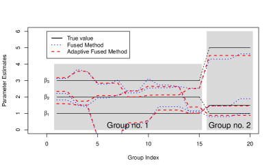
(a) Least Squares Error

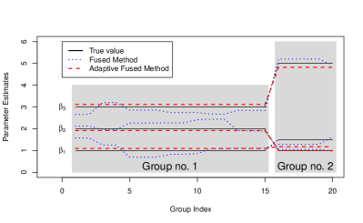
(b) Quantile Check Function

Figure 1: An illustration of the model in (1) for two truly different successive groups (out of $g=20$ in total) and three explanatory variables in each group ($p=3$). The first group specific vector parameter is the same for the groups $j\in\{1,\dots,15\}$ and it differs from the second group specific vector parameter, which is the same for the groups $j\in\{16\dots,20\}$. The Cauchy error terms are considered to visualize the robust favor of the quantile estimation approach for $\tau=0.5$ (right panel) when compared with the standard least squares (left panel).

$\boldsymbol{\mathcal{D}}$		$\boldsymbol{p=1}$	Model with 2 different groups			Model with 5 different groups			Model with 10 different groups			Model with $\boldsymbol{20~{}\%}$ different groups
		$\boldsymbol{g=n}$	MED	MAD	Recovery	MED	MAD	Recovery	MED	MAD	Recovery	MED	MAD	Recovery
$\boldsymbol{N}$		20	0.01	0.17	0.91$/$12.25	0.00	0.19	0.99$/$3.19	0.04	0.24	0.90$/$1.53	0.00	0.19	0.93$/$4.17
	$\widehat{{\textrm{$\mathbf{\beta}$}}^{g}}_{\!\!(LS)}$	100	0.00	0.09	1.00$/$71.48	-0.01	0.09	1.00$/$18.02	0.00	0.10	0.99$/$8.07	0.01	0.12	0.98$/$4.01
		200	0.01	0.07	1.00$/$152	0.00	0.07	1.00$/$38.24	0.00	0.07	1.00$/$17.14	0.00	0.08	1.00$/$4.07
		20	-0.05	0.10	0.64$/$1.26	0.01	0.16	0.87$/$0.93	0.06	0.31	0.59$/$0.66	-0.04	0.14	0.72$/$0.83
	$\overset{\vee}{{\textrm{$\mathbf{\beta}$}}^{g}}_{\!\!(aLS)}$	100	0.00	0.02	0.93$/$1.84	-0.06	0.03	0.98$/$1.12	0.02	0.06	0.94$/$1.08	-0.12	0.12	0.81$/$0.94
		200	0.00	0.01	0.99$/$2.15	0.02	0.01	1.00$/$1.13	-0.02	0.02	0.99$/$1.09	0.06	0.08	0.90$/$0.92
		20	0.01	0.12	0.88$/$6.44	-0.03	0.17	0.98$/$2.02	0.22	0.27	0.82$/$1.16	-0.01	0.15	0.91$/$2.59
	$\widehat{{\textrm{$\mathbf{\beta}$}}^{g}}$	100	0.00	0.07	1.00$/$48.99	-0.02	0.07	1.00$/$12.67	0.01	0.08	0.99$/$5.86	0.02	0.10	0.97$/$3.06
		200	0.00	0.05	1.00$/$115	0.01	0.05	1.00$/$29.27	0.00	0.06	1.00$/$13.16	0.01	0.07	1.00$/$3.29
		20	-0.22	0.18	0.00$/$0.00	-0.50	0.55	0.39$/$0.39	0.52	0.97	0.23$/$0.24	-0.12	0.55	0.31$/$0.31
	$\overset{\vee}{{\textrm{$\mathbf{\beta}$}}^{g}}$	100	-0.05	0.08	0.82$/$0.91	-0.33	0.13	0.51$/$0.51	0.34	0.35	0.42$/$0.42	-0.34	0.47	0.18$/$0.18
		200	0.00	0.02	0.98$/$1.02	0.20	0.07	0.92$/$0.92	-0.15	0.20	0.84$/$0.84	0.24	0.45	0.44$/$0.44
$\boldsymbol{C}$		20	0.01	53.93	0.92$/$16.37	-0.12	60.79	0.93$/$4.05	0.09	19.27	0.89$/$1.82	0.03	25.92	0.92$/$5.42
	$\widehat{{\textrm{$\mathbf{\beta}$}}^{g}}_{\!\!(LS)}$	100	0.05	143	0.96$/$92.47	0.02	45.18	0.95$/$23.16	0.02	74.57	0.95$/$10.26	0.00	73.24	0.95$/$4.90
		200	0.00	38.55	0.97$/$190	0.01	34.36	0.96$/$47.66	-0.02	57.97	0.97$/$21.20	0.05	71.76	0.96$/$4.90
		20	1.72	62.95	0.63$/$10.50	1.54	81.97	0.73$/$2.74	1.82	20.97	0.67$/$1.31	1.70	27.58	0.71$/$3.60
	$\overset{\vee}{{\textrm{$\mathbf{\beta}$}}^{g}}_{\!\!(aLS)}$	100	-1.51	456	0.74$/$68.01	-1.56	51.66	0.76$/$17.13	-1.48	88.17	0.76$/$7.64	-1.54	137	0.75$/$3.68
		200	-1.16	43.63	0.80$/$148	-1.14	36.66	0.79$/$37.09	-1.15	70.54	0.80$/$16.54	-1.13	88.10	0.80$/$3.88
		20	0.00	0.22	0.64$/$6.15	-0.05	0.35	0.84$/$1.90	0.33	0.49	0.66$/$0.97	-0.03	0.31	0.76$/$2.44
	$\widehat{{\textrm{$\mathbf{\beta}$}}^{g}}$	100	0.00	0.13	0.85$/$48.71	-0.03	0.15	0.95$/$12.58	0.02	0.17	0.89$/$5.73	0.01	0.21	0.81$/$2.90
		200	0.00	0.12	0.93$/$115	0.00	0.13	0.98$/$29.12	-0.01	0.13	0.95$/$13.09	0.01	0.18	0.94$/$3.23
		20	-0.22	0.20	0.01$/$0.01	-0.80	0.77	0.28$/$0.30	0.75	1.17	0.16$/$0.19	-0.41	0.74	0.20$/$0.21
	$\overset{\vee}{{\textrm{$\mathbf{\beta}$}}^{g}}$	100	-0.04	0.11	0.41$/$1.03	-0.34	0.14	0.51$/$0.53	0.32	0.35	0.39$/$0.44	-0.34	0.47	0.19$/$0.20
		200	-0.04	0.04	0.62$/$1.96	0.30	0.11	0.65$/$0.69	-0.16	0.26	0.60$/$0.74	0.38	0.52	0.39$/$0.40

Table 1: Simulation results for the situation where the dimension of the unknown parameter is $p=1$. Two goodness-of-fit quantities are provided: the median (MED) of $(Y_{i}-\widehat{Y}_{i})_{1\leqslant i\leqslant n}$ and the mean absolute difference (MAD) between the true parameter vector $\boldsymbol{\beta}^{0}$ and the corresponding empirical estimate $\widehat{\boldsymbol{\beta}}$. The Recovery column is given in terms of two values: the proportion of truly discovered different successive coefficients (value $1$ stands for all true changes being discovered) and the proportion between the number of estimated different successive coefficients and true changes (value $1$ stands for the situation where the number of estimated changes equals the number of true changes). An ideal situation is $1.00/1.00$ which means that all true changes are discovered with no other detections in addition. The results are averaged over 1000 Monte Carlo simulation runs.

$\boldsymbol{\mathcal{D}}$		$\boldsymbol{p=3}$	Model with 2 different groups			Model with 5 different groups			Model with 10 different groups			Model with $\boldsymbol{20~{}\%}$ different groups
		$\boldsymbol{g=n/p}$	MED	MAD	Recovery	MED	MAD	Recovery	MED	MAD	Recovery	MED	MAD	Recovery
$\boldsymbol{N}$		20	-0.03	0.17	1.00$/$9.87	0.02	0.40	0.92$/$2.63	0.02	1.00	0.65$/$1.11	-0.01	0.34	0.76$/$3.37
	$\widehat{{\textrm{$\mathbf{\beta}$}}^{g}}_{\!\!(LS)}$	100	0.00	0.05	1.00$/$62.67	0.00	0.06	1.00$/$15.61	0.00	0.08	1.00$/$6.72	0.00	0.14	1.00$/$3.03
		200	0.00	0.02	1.00$/$87.79	0.00	0.03	1.00$/$20.40	-0.07	0.07	1.00$/$11.03	0.00	0.10	1.00$/$2.50
		20	-0.02	0.08	0.99$/$1.82	0.07	0.44	0.63$/$1.31	-0.02	1.09	0.39$/$0.64	-0.05	0.37	0.41$/$1.65
	$\overset{\vee}{{\textrm{$\mathbf{\beta}$}}^{g}}_{\!\!(aLS)}$	100	0.00	0.01	1.00$/$2.00	0.00	0.02	1.00$/$1.13	0.00	0.03	1.00$/$1.04	0.04	0.08	0.97$/$1.12
		200	0.00	0.01	1.00$/$1.26	0.00	0.01	1.00$/$1.02	0.00	0.02	1.00$/$1.17	0.02	0.05	0.99$/$1.02
		20	-0.04	0.18	1.00$/$9.92	0.00	0.41	0.92$/$2.70	0.08	1.01	0.57$/$1.02	-0.01	0.35	0.77$/$3.48
	$\widehat{{\textrm{$\mathbf{\beta}$}}^{g}}$	100	-5.79	2.05	1.00$/$99.00	-8.29	2.47	1.00$/$24.75	-4.86	0.91	1.00$/$10.08	0.05	0.17	1.00$/$4.28
		200	-0.01	0.02	1.00$/$29.92	0.00	0.02	1.00$/$8.44	-0.02	0.03	1.00$/$4.73	-0.06	0.36	0.82$/$1.76
		20	0.03	0.24	0.85$/$0.90	0.00	0.53	0.33$/$0.63	-0.16	1.15	0.29$/$0.38	-0.07	0.61	0.22$/$0.89
	$\overset{\vee}{{\textrm{$\mathbf{\beta}$}}^{g}}$	100	0.06	0.07	0.07$/$2.57	-0.09	0.13	0.80$/$3.06	-0.21	0.15	0.88$/$1.31	-0.07	0.38	0.70$/$0.72
		200	0.00	0.01	1.00$/$1.00	-0.01	0.01	1.00$/$1.00	0.00	0.02	1.00$/$1.00	-0.15	0.51	0.51$/$0.69
$\boldsymbol{C}$		20	0.00	3.24	0.73$/$10.85	0.01	3.26	0.70$/$2.73	0.01	3.54	0.65$/$1.21	0.00	3.05	0.65$/$3.67
	$\widehat{{\textrm{$\mathbf{\beta}$}}^{g}}_{\!\!(LS)}$	100	-0.08	3.36	0.86$/$71.60	0.05	3.18	0.83$/$17.35	-0.22	3.12	0.82$/$7.64	-0.01	3.16	0.81$/$3.55
		200	-0.03	2.29	0.79$/$128	-0.10	2.29	0.82$/$31.83	-0.12	2.30	0.80$/$14.52	-0.16	2.42	0.79$/$3.24
		20	1.69	3.54	0.57$/$6.26	1.76	3.45	0.45$/$1.64	1.74	3.91	0.45$/$0.78	1.71	3.37	0.42$/$2.20
	$\overset{\vee}{{\textrm{$\mathbf{\beta}$}}^{g}}_{\!\!(aLS)}$	100	-2.04	3.60	0.68$/$35.92	-1.65	3.32	0.62$/$9.17	-1.58	3.29	0.62$/$4.23	-1.53	3.42	0.58$/$1.99
		200	-1.22	2.49	0.67$/$75.66	-1.11	2.49	0.67$/$18.97	-1.17	2.54	0.65$/$8.49	-1.16	2.68	0.62$/$2.01
		20	-0.02	0.55	0.76$/$9.84	0.02	0.71	0.65$/$2.53	0.05	1.17	0.56$/$1.09	0.00	0.73	0.62$/$3.40
	$\widehat{{\textrm{$\mathbf{\beta}$}}^{g}}$	100	-8.20	2.03	1.00$/$97.88	-9.66	2.30	1.00$/$24.61	-7.85	1.62	0.98$/$10.38	-0.63	0.67	0.97$/$4.89
		200	-2.66	0.39	1.00$/$109	-2.45	0.40	1.00$/$27.59	-1.27	0.22	1.00$/$6.18	-1.12	0.57	0.77$/$1.87
		20	-0.02	0.48	0.32$/$1.34	0.12	0.71	0.22$/$0.71	-0.17	1.28	0.22$/$0.35	0.02	0.75	0.23$/$1.00
	$\overset{\vee}{{\textrm{$\mathbf{\beta}$}}^{g}}$	100	-0.11	0.12	0.48$/$9.37	-0.56	0.26	0.67$/$5.14	-0.58	0.39	0.49$/$1.61	-0.24	0.60	0.37$/$0.71
		200	-0.52	0.06	0.99$/$8.28	-0.26	0.07	0.89$/$2.41	-0.41	0.11	0.95$/$1.48	-0.32	0.60	0.43$/$0.66

Table 2: Simulation results for the situation where the dimension of the unknown parameter is $p=3$. Two goodness-of-fit quantities are provided: the median (MED) of $(Y_{i}-\widehat{Y}_{i})_{1\leqslant i\leqslant n}$ and the mean absolute difference (MAD) between the true parameter vector $\boldsymbol{\beta}^{0}$ and the corresponding empirical estimate $\widehat{\boldsymbol{\beta}}$. The Recovery column is given in terms of two values: the proportion of truly discovered different successive coefficient groups (value $1$ stands for all true changes being discovered) and the proportion between the number of estimated different successive coefficient groups and true changes (value $1$ stands for the situation where the number of estimated changes equals the number of true changes). An ideal situation is $1.00/1.00$ which means that all true changes are discovered with no other detections in addition. The results are averaged over 1000 Monte Carlo simulation runs.

From Tables 1 and 2 for the Gaussian errors, we deduce that for $|{\cal B}^{0}|\in\{2,5,10\}$, the fused estimations for the least squares and the quantile methods have the same properties and the same also applies for the adaptive frameworks which, moreover, have the recovery detection rates close to one. On the other hand, if the assumption $|{\cal B}^{0}|<\infty$ does not hold, as for the models with $20\%$ different successive groups, then not all of the different successive groups are detected and the performance is worse.

The robustness of the quantile methods is obvious when the Cauchy errors are used instead: while the LS based methods fail in both, the estimation and the group detection, the quantile approaches perform comparably well as in the situations with the Gaussian errors.

4.2 Application to Air Quality data

In order to demonstrate the practical applicability of the proposed model we use the air quality data from De Vito et al. (2009) which can be downloaded from the Machine Learning Repository site http://archive.ics.uci.edu/ml/datasets/Air+Quality#. The hourly meteorological and air quality data were recorded from March 2004 to February 2005. The idea is to use the daily temperature and humidity profiles (recorded every hours) to predict the maximum benzene concentration level for the given day. Optimally, it would be appropriate to use the temperature and humidity information only from some few instant moments during the day instead of recording both continuous profiles over the whole day. Given the data, there are $g=24$ hourly groups and for each group there is the corresponding vector parameter $\boldsymbol{\beta}_{j}=(\beta_{j}^{T},\beta_{j}^{H})^{\top}\in\mathbb{R}^{2}$, for $j=1,\dots,24$, where $\beta_{j}^{T}$ is responsible for the contribution of the temperature at ’$j$’ o’clock and $\beta_{j}^{H}$ models the effect of the humidity, again at ’$j$’ o’clock. Using the model formulation from Section 2 and the estimation in terms of (5) it can be achieved that most of the corresponding parameter vector estimates are the same. If otherwise, then the existing changes in the vector estimates identify some specific daily segments with the same temperature and humidity contribution with respect to the maximum daily benzene concentration. The corresponding magnitudes for both effects in each daily segment are all estimated simultaneously.

Similarly as in the simulation section, four different models are fitted: the fused group LS approach and its adaptive version both presented in Figures 3(a) and 3(a) and the proposed fused group quantile and the adaptive fused group quantile in Figures 3(c) and 3(d). The temperature data and the humidity data are heavily skewed and, therefore, it can be assumed that robust approaches are more appropriate for this situation.

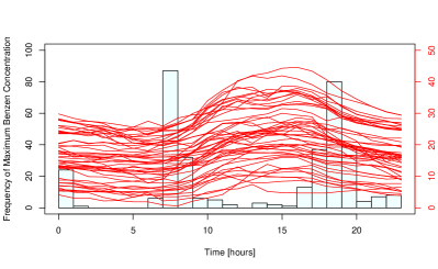
(a) Daily temperature

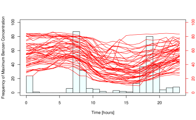
(b) Daily humidity

Figure 2: Daily temperature profiles (left panel) and daily humidity profiles (right panel) for 50 randomly selected days out of 357 available days with full profiles in total. In addition, the maximum benzene concentration is recorded for each day and the corresponding time of the maximum occurrence (in hours) is given in terms of the frequency histograms in both panels.

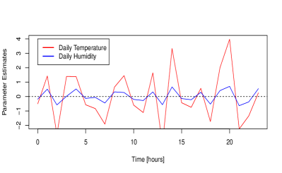
(a) Fused group LS solution

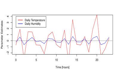
(b) Adaptive fused group LS solution

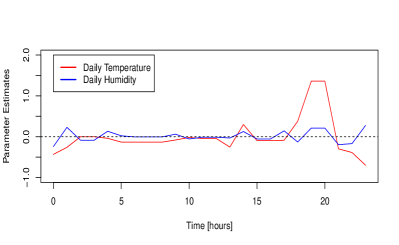
(c) Fused group quantile solution

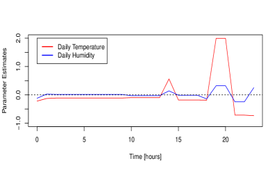
(d) Adaptive fused group quantile solution

Figure 3: The estimated parameter vectors $\widehat{\boldsymbol{\beta}}_{j}=(\widehat{\beta}_{j}^{T},\widehat{\beta}_{j}^{H})^{\top}\in\mathbb{R}^{2}$, for $j=1,\dots,24$, for four different estimation techniques: fused group LS, adaptive fused group LS, fused group quantile and adaptive fused group quantile. The adaptive fused group quantile estimator in panel (d) clearly identifies some instant moments during a day when the temperature and humidity information is relevant for the maximum benzene concentration. In other words, it seems enough to record the temperature and humidity information at 2 pm and, also, after 6 pm.

Indeed, while the fused group LS and also its adaptive version can not identify any specific daily moments which should be used to determine the maximum daily benzene concentration, the fused group quantile and its adaptive version in particular clearly identify some segments during the day when the contribution of the temperature and humidity is obvious.

5 Proofs

Throughout the proofs, the following identity for the quantile check function $\rho_{\tau}$ is be used: for any $x,y\in\mathbb{R}$ it holds that

$$\rho_{\tau}(x-y)-\rho_{\tau}(x)=y(1\!\!1_{x<0}-\tau)+\int^{\tau}_{0}(1\!\!1_{x\leq v}-\mathbf{{u}}_{x\leq 0})dv.$$ (13)

Proof of Lemma 3.1.
We will show that for all $\epsilon>0$, there exists a constant $C_{\epsilon}>0$, such that for $n$ large enough, we have

$$\mathbb{P}\left[\inf_{\mathbf{{u}}\in\mathbb{R}^{r_{n}},\|\mathbf{{u}}\|_{1}=1}G_{n}\big{(}\textrm{$\mathbf{\beta^{0}}$}+C_{\epsilon}b_{n}\mathbf{{u}}\big{)}>G_{n}(\textrm{$\mathbf{\beta^{0}}$})\right]\geq 1-\epsilon.$$ (14)

Then, for any constant $c_{1}>0$, we can write the difference $G_{n}\big{(}\textrm{$\mathbf{\beta^{0}}$}+c_{1}b_{n}\mathbf{{u}}\big{)}-G_{n}(\textrm{$\mathbf{\beta^{0}}$})$ using the form

$$G_{n}\big{(}\textrm{$\mathbf{\beta^{0}}$}+c_{1}b_{n}\mathbf{{u}}\big{)}-G_{n}(\textrm{$\mathbf{\beta^{0}}$})=\mathbb{E}\,\big{[}G_{n}\big{(}\textrm{$\mathbf{\beta^{0}}$}+c_{1}b_{n}\mathbf{{u}}\big{)}-G_{n}(\textrm{$\mathbf{\beta^{0}}$})\big{]}+{\bf W}_{n}^{\top}\mathbf{{u}}+\sum^{n}_{i=1}({\cal R}_{i}-\mathbb{E}\,[{\cal R}_{i}]),$$ (15)

with the $r_{n}$-dimensional random vector ${\bf W}_{n}\equiv c_{1}b_{n}\sum^{n}_{i=1}{\cal D}_{i}\mathbb{X}_{i}$, the random variables ${\cal D}_{i}\equiv(1-\tau)1\!\!1_{\{\varepsilon_{i}<0\}}-\tau 1\!\!1_{\{\varepsilon_{i}\geq 0\}}$, and ${\cal R}_{i}\equiv\rho_{\tau}(\varepsilon_{i}-c_{1}b_{n}\mathbb{X}_{i}^{\top}\mathbf{{u}})-\rho_{\tau}(\varepsilon_{i})-c_{1}b_{n}{\cal D}_{i}\mathbb{X}_{i}^{\top}\mathbf{{u}}$.

Using the Holder’s inequality, we have that $|\mathbb{X}_{i}^{\prime}\mathbf{{u}}|\leq\|\mathbb{X}_{i}\|_{\infty}\|\mathbf{{u}}\|_{1}$. Then, for all $\mathbf{{u}}\in\mathbb{R}^{r_{n}}$ such that $\|\mathbf{{u}}\|_{1}=1$, by Assumption (A1), we have that $|\mathbb{X}_{i}^{\top}\mathbf{{u}}|\leq C$.

Firstly, we study the first term on the right-hand side of relation (15). Using the identity in (13), we obtain

$$G_{n}\big{(}\textrm{$\mathbf{\beta^{0}}$}+c_{1}b_{n}\mathbf{{u}}\big{)}-G_{n}(\textrm{$\mathbf{\beta^{0}}$})=-c_{1}b_{n}\sum^{n}_{i=1}\mathbb{X}_{i}^{\top}\mathbf{{u}}{\cal D}_{i}+\sum^{n}_{i=1}\int_{0}^{c_{1}b_{n}\mathbb{X}_{i}^{\top}\mathbf{{u}}}[1\!\!1_{\{\varepsilon_{i}<v\}}-1\!\!1_{\{\varepsilon_{i}<0\}}]dv.$$

Applying now the mean value theorem, taking into account the fact that the derivative of $f$ is bounded in a neighborhood of zero by Assumption (A3), and the fact that $\|\mathbf{{u}}\|_{1}=1$, $\mathbb{E}\,[{\cal D}_{i}]=0$ and $b_{n}\rightarrow 0$, we obtain

$$\mathbb{E}\,\big{[}G_{n}\big{(}\textrm{$\mathbf{\beta^{0}}$}+c_{1}b_{n}\mathbf{{u}}\big{)}-G_{n}(\textrm{$\mathbf{\beta^{0}}$})\big{]} =\sum^{n}_{i=1}\mathbb{E}\,\Big{[}\int_{0}^{c_{1}b_{n}\mathbb{X}_{i}^{\top}\mathbf{{u}}}1\!\!1_{\{0<\varepsilon_{i}<v\}}\Big{]}dv$$

$$=\sum^{n}_{i=1}\int_{0}^{c_{1}b_{n}\mathbb{X}_{i}^{\top}\mathbf{{u}}}[F(v)-F(0)]dv$$

$$=\frac{f(0)}{2}c^{2}_{1}b^{2}_{n}\sum^{n}_{i=1}(\mathbb{X}_{i}^{\top}\mathbf{{u}})^{2}+o\Big{(}b^{2}_{n}\sum^{n}_{i=1}\mathbf{{u}}^{\top}(\mathbb{X}_{i}\mathbb{X}_{i}^{\top})\mathbf{{u}}\Big{)}.$$

Using Assumption (A2) together with $f(0)>0$, we get that

$$n^{-1}\mathbb{E}\,\big{[}G_{n}\big{(}\textrm{$\mathbf{\beta^{0}}$}+c_{1}b_{n}\mathbf{{u}}\big{)}-G_{n}(\textrm{$\mathbf{\beta^{0}}$})\big{]}=Cf(0)b^{2}_{n}\frac{1}{n}\sum^{n}_{i=1}\mathbf{{u}}^{\top}\mathbb{X}_{i}\mathbb{X}^{\top}_{i}\mathbf{{u}}(1+o(1))>0.$$ (16)

Next, we study the last two terms on the right-hand side of relation (15). For the last term we have, with probability one, for any $i=1,\dots,n$, that $|{\cal R}_{i}|\leq c_{1}b_{n}|\mathbb{X}_{i}^{\top}\mathbf{{u}}|1\!\!1_{\{|\varepsilon_{i}|\leq c_{1}b_{n}|\mathbb{X}_{i}^{\top}\mathbf{{u}}|\}}$. Since $(\varepsilon_{i})_{1\leqslant i\leqslant n}$ are independent, then the random variables $({\cal R}_{i})_{1\leqslant i\leqslant n}$ are independent as well and, therefore

$$\mathbb{E}\,\big{[}\sum^{n}_{i=1}({\cal R}_{i}-\mathbb{E}\,[{\cal R}_{i}])\big{]}^{2} =\sum^{n}_{i=1}\mathbb{E}\,[{\cal R}_{i}-\mathbb{E}\,[{\cal R}_{i}]]^{2}$$ (17)

$$\leq\sum^{n}_{i=1}\mathbb{E}\,[{\cal R}_{i}^{2}]\leq Cb_{n}^{2}\sum^{n}_{i=1}|\mathbb{X}_{i}^{\top}\mathbf{{u}}|^{2}\mathbb{E}\,\big{[}1\!\!1_{\{|\varepsilon_{i}|\leq c_{1}b_{n}|\mathbb{X}_{i}^{\top}\mathbf{{u}}|\}}\big{]}.$$

Using the fact that the density $f$ is bounded in a neighborhood of $0$ by assumption (A3), adopting the Taylor’s expansion, Cauchy-Schwarz and Holder inequalities, Assumption (A1), and the fact that $\|\mathbf{{u}}\|_{1}=1$, we obtain

$$\mathbb{E}\,\Big{[}1\!\!1_{\{|\varepsilon_{i}|\leq c_{1}b_{n}|\mathbb{X}_{i}^{\top}\mathbf{{u}}|\}}\Big{]}=2c_{1}b_{n}|\mathbb{X}_{i}^{\top}\mathbf{{u}}|f(d_{i,n})\leq Cb_{n}\max_{1\leqslant i\leqslant n}\|\mathbb{X}_{i}\|_{\infty}=Cb_{n},$$ (18)

with $d_{i,n}$ between $c_{1}b_{n}|\mathbb{X}_{i}^{\top}\mathbf{{u}}|$ and $(-c_{1}b_{n}|\mathbb{X}_{i}^{\top}\mathbf{{u}}|)$. Then, using Assumption (A1) together with the relations in (17) and (18), and the fact that $|\mathbb{X}_{i}^{\top}\mathbf{{u}}|\leq C$, we have

$$\mathbb{E}\,\Big{[}\sum^{n}_{i=1}({\cal R}_{i}-\mathbb{E}\,[{\cal R}_{i}])\Big{]}^{2}\leq Cb^{3}_{n}\sum^{n}_{i=1}(\mathbb{X}_{i}^{\top}\mathbf{{u}})^{2}=O(nb^{3}_{n}).$$ (19)

We consider a deterministic sequence $(a_{n})_{n\in\mathbb{N}}$ such that: $a_{n}\rightarrow\infty$ and $nb_{n}^{3}\ll a_{n}\ll n^{2}b^{4}_{n}$. An example of such sequence is $a_{n}=(\log n)^{3/2}$ if $b_{n}=\big{(}n^{-1}\log n\big{)}^{1/2}$.
Considering the relation in (19) and since $a_{n}\gg nb_{n}^{3}$, then also

$$\mathbb{E}\,[a_{n}^{-1}\big{(}\sum^{n}_{i=1}({\cal R}_{i}-\mathbb{E}\,[{\cal R}_{i}])\big{)}^{2}]=O(a_{n}^{-1}nb^{3}_{n})=o(1),$$

which implies, by the Bienaymé-Tchebychev inequality, that the last term of the right-hand side of the relation in (15) equals to

$$\sum^{n}_{i=1}({\cal R}_{i}-\mathbb{E}\,[{\cal R}_{i}])=o_{\mathbb{P}}(a_{n}^{1/2}).$$ (20)

Finally, we study the second term of the right-hand side in (15). By the Central Limit Theorem (CLT) for the independent random variables $({\cal D}_{i}\mathbb{X}_{i}^{\top}\mathbf{{u}})_{1\leqslant i\leqslant n}$, we get ${\bf W}_{n}^{\top}\mathbf{{u}}=O_{\mathbb{P}}(n^{1/2}b_{n})$. Using now the fact that $n^{-1}\sum^{n}_{i=1}\mathbf{{u}}^{\top}\mathbb{X}_{i}\mathbb{X}_{i}^{\top}\mathbf{{u}}$ is bounded by Assumption (A2), and by the condition in (2) where $n^{1/2}b_{n}\rightarrow\infty$, since $a_{n}\ll n^{2}b_{n}^{4}$, together with the relations in (16) and (20), we have for (15) the following:

$$G_{n}\big{(}\textrm{$\mathbf{\beta^{0}}$}+c_{1}b_{n}\mathbf{{u}}\big{)}-G_{n}(\textrm{$\mathbf{\beta^{0}}$})=Cnb^{2}_{n}\Bigg{(}n^{-1}\sum^{n}_{i=1}\mathbf{{u}}^{\top}\mathbb{X}_{i}\mathbb{X}_{i}^{\top}\mathbf{{u}}\Bigg{)}\big{(}1+o_{\mathbb{P}}(1)\big{)}>0,$$

Therefore, the relation in (14) is proved. Moreover, it implies that $\|\widetilde{{\textrm{$\mathbf{\beta}$}}^{g}}-\textrm{$\mathbf{\beta^{0}}$}\|_{1}=O_{\mathbb{P}}(b_{n})$ and, therefore, the lemma is proved. $\blacksquare$

Proof of Theorem 3.3.
In order to prove the assertion of the theorem, let us consider a vector $\mathbf{{u}}\in\mathbb{R}^{r_{n}}$, such that $\|\mathbf{{u}}\|_{1}=1$ and a constant $c_{2}>0$. Then the following holds

$$\begin{split}Q_{n}(\textrm{$\mathbf{\beta^{0}}$}+c_{2}b_{n}\mathbf{{u}})-Q_{n}(\textrm{$\mathbf{\beta^{0}}$})=G_{n}(\textrm{$\mathbf{\beta^{0}}$}+c_{2}b_{n}\mathbf{{u}})-G_{n}(\textrm{$\mathbf{\beta^{0}}$})\qquad\qquad\qquad\qquad\\ +n\lambda_{n}\sum^{g}_{j=2}\left[\big{\|}\textrm{$\mathbf{\beta}$}^{0}_{j}+c_{2}b_{n}\mathbf{{u}}_{j}-(\textrm{$\mathbf{\beta}$}^{0}_{j-1}+c_{2}b_{n}\mathbf{{u}}_{j-1})\big{\|}_{q}-\|\textrm{$\mathbf{\beta}$}^{0}_{j}-\textrm{$\mathbf{\beta}$}^{0}_{j-1}\|_{q}\right].\end{split}$$ (21)

On the other hand, since $\|\mathbf{{u}}\|_{2}\leq\|\mathbf{{u}}\|_{1}=1$, by the proof of Lemma 3.1, we have with the probability converging to 1, that

$$G_{n}(\textrm{$\mathbf{\beta^{0}}$}+c_{2}b_{n}\mathbf{{u}})-G_{n}(\textrm{$\mathbf{\beta^{0}}$})\geq c_{2}nb_{n}^{2}\Big{(}n^{-1}\sum^{n}_{i=1}\mathbf{{u}}^{\top}\mathbb{X}_{i}\mathbb{X}_{i}^{\top}\mathbf{{u}}\Big{)}\geq Cnb_{n}^{2}>0.$$ (22)

If the components of $\mathbf{{u}}$ are denoted as $\mathbf{{u}}_{1},\cdots,\mathbf{{u}}_{g}$, then, using the triangular inequality, for the penalty in (21), we have

$$n\lambda_{n}\sum^{g}_{j=2} \left[\big{\|}\textrm{$\mathbf{\beta}$}^{0}_{j}+c_{2}b_{n}\mathbf{{u}}_{j}-(\textrm{$\mathbf{\beta}$}^{0}_{j-1}+c_{2}b_{n}\mathbf{{u}}_{j-1})\big{\|}_{q}-\|\textrm{$\mathbf{\beta}$}^{0}_{j}-\textrm{$\mathbf{\beta}$}^{0}_{j-1}\|_{q}\right]$$

$$\geq n\lambda_{n}\sum_{j\in{\cal B}^{0}}\left[\big{\|}\textrm{$\mathbf{\beta}$}^{0}_{j}+c_{2}b_{n}\mathbf{{u}}_{j}-(\textrm{$\mathbf{\beta}$}^{0}_{j-1}+c_{2}b_{n}\mathbf{{u}}_{j-1})\big{\|}_{q}-\|\textrm{$\mathbf{\beta}$}^{0}_{j}-\textrm{$\mathbf{\beta}$}^{0}_{j-1}\|_{q}\right]$$

$$\geq-c_{2}n\lambda_{n}b_{n}\sum_{j\in{\cal B}^{0}}\|\mathbf{{u}}_{j}-\mathbf{{u}}_{j-1}\|_{q}=-Cc_{2}n\lambda_{n}b_{n},$$ (23)

where for the last equality in (23) we have used the fact that

$$\|\mathbf{{u}}_{j}-\mathbf{{u}}_{j-1}\|_{q}\leq\|\mathbf{{u}}_{j}-\mathbf{{u}}_{j-1}\|_{1}\leq\|\mathbf{{u}}_{j}\|_{1}+\|\mathbf{{u}}_{j-1}\|_{1},$$

together with $\|\mathbf{{u}}\|_{1}=1$ and $|{\cal B}^{0}|<\infty$. Since $\lambda_{n}b_{n}^{-1}\rightarrow 0$, as $n\rightarrow\infty$, then also $n\lambda_{n}b_{n}=o(nb_{n}^{2})$ and taking into account the relation in (22), we obtain for (21) and (23) that

$$Q_{n}(\textrm{$\mathbf{\beta^{0}}$}+c_{2}b_{n}\mathbf{{u}})>Q_{n}(\textrm{$\mathbf{\beta^{0}}$}),$$

which holds with the probability converging to 1, as $n\rightarrow\infty$. $\blacksquare$

Proof of Theorem 3.4.
By Theorem 3.3 we have

$$\lim_{n\rightarrow\infty}\mathbb{P}\Big{[}\widehat{{\textrm{$\mathbf{\beta}$}}^{g}}=\mathop{\mathrm{arg\,min}}_{\textrm{$\mathbf{\beta}$}^{g}\in{\cal V}_{n}(\textrm{$\mathbf{\beta}$}^{0})}\big{(}Q_{n}(\textrm{$\mathbf{\beta}$}^{g})-Q_{n}(\textrm{$\mathbf{\beta}$}^{0})\big{)}\Big{]}=1,$$ (24)

with the neighborhood ${\cal V}_{n}(\textrm{$\mathbf{\beta}$}^{0})$ of $\mathbf{\beta^{0}}$ with the radius $c_{2}b_{n}$ defined as

$${\cal V}_{n}(\textrm{$\mathbf{\beta}$}^{0})\equiv\big{\{}\textrm{$\mathbf{\beta}$}^{g}\in\mathbb{R}^{r_{n}};\|\textrm{$\mathbf{\beta}$}^{g}-\textrm{$\mathbf{\beta}$}^{0}\|_{1}\leq c_{2}b_{n}\big{\}},$$

for some constant $c_{2}>0$. Then, in order to prove the assertion of the theorem we consider the parameter vector $\textrm{$\mathbf{\beta}$}^{g}=(\textrm{$\mathbf{\beta}$}_{1}^{\top},\dots,\textrm{$\mathbf{\beta}$}_{g}^{\top})\in{\cal V}_{n}(\textrm{$\mathbf{\beta}$}^{0})$ and the index set ${\cal B}\equiv\big{\{}j\in\{2,\cdots,g\};\textrm{$\mathbf{\beta}$}_{j}\neq\textrm{$\mathbf{\beta}$}_{j-1}\big{\}}$. Note, that ${\cal B}$ and $\textrm{$\mathbf{\beta}$}^{g}$ both depend on $n$ and the vector of true unknown parameters $\textrm{$\mathbf{\beta}$}^{g}$ is not random. Therefore, we consider only ${\cal B}\cap\overline{{\cal B}^{0}}\neq\emptyset$, otherwise the theorem trivially holds.

Let us concentrate on the following decomposition:

$$Q_{n}(\textrm{$\mathbf{\beta}$}^{g})-Q_{n}(\textrm{$\mathbf{\beta}$}^{0}) = \sum^{n}_{i=1}\left[\rho_{\tau}(Y_{i}-\mathbb{X}_{i}^{\top}\textrm{$\mathbf{\beta}$}^{g})-\rho_{\tau}(Y_{i}-\mathbb{X}_{i}^{\top}\textrm{$\mathbf{\beta}$}^{0})\right]$$ (25)

$$\qquad+n\lambda_{n}\sum_{j\in{\cal B}\cap{\cal B}^{0}}\big{[}\|\textrm{$\mathbf{\beta}$}_{j}-\textrm{$\mathbf{\beta}$}_{j-1}\|_{q}-\|\textrm{$\mathbf{\beta}$}^{0}_{j}-\textrm{$\mathbf{\beta}$}^{0}_{j-1}\|_{q}\big{]}$$

$$\qquad+n\lambda_{n}\sum_{j\in{\cal B}\cap\overline{{\cal B}^{0}}}\|\textrm{$\mathbf{\beta}$}_{j}-\textrm{$\mathbf{\beta}$}_{j-1}\|_{q}-n\lambda_{n}\sum_{j\in\overline{{\cal B}}\cap{\cal B}^{0}}\|\textrm{$\mathbf{\beta}$}^{0}_{j}-\textrm{$\mathbf{\beta}$}^{0}_{j-1}\|_{q}$$

$$\equiv S_{1n}+S_{2n}+S_{3n}-S_{4n}.$$

Using the identity in (13) we can write the sum $S_{1n}$ as

$$S_{1n} =\sum^{n}_{i=1}(\textrm{$\mathbf{\beta}$}^{g}-\textrm{$\mathbf{\beta}$}^{0})^{\top}\mathbb{X}_{i}\big{[}1\!\!1_{\{Y_{i}-\mathbb{X}_{i}^{\top}\textrm{$\mathbf{\beta}$}^{0}\leq 0\}}-\tau\big{]}$$

$$\qquad+\sum^{n}_{i=1}\int^{\mathbb{X}_{i}^{\top}(\textrm{$\mathbf{\beta}$}^{g}-\textrm{$\mathbf{\beta}$}^{0})}_{0}\Big{[}1\!\!1_{\{Y_{i}-\mathbb{X}_{i}^{\top}\textrm{$\mathbf{\beta}$}^{0}\leq v\}}-1\!\!1_{\{Y_{i}-\mathbb{X}_{i}^{\top}\textrm{$\mathbf{\beta}$}^{0}\leq 0\}}\Big{]}dv$$

$$\equiv T_{1n}+T_{2n}.$$ (26)

For $T_{1n}$, we have $\mathbb{E}\,[T_{1n}]=\sum^{n}_{i=1}(\textrm{$\mathbf{\beta}$}^{g}-\textrm{$\mathbf{\beta}$}^{0})^{\top}\mathbb{X}_{i}\big{[}F(0)-F(0)\big{]}=0$ and using Assumptions (A1), (A2), and (A3), we obtain for the variance that

$$\mathbb{V}\mbox{ar}\,[T_{1n}]=\tau(1-\tau)\sum^{n}_{i=1}\big{(}(\textrm{$\mathbf{\beta}$}^{g}-\textrm{$\mathbf{\beta}$}^{0})^{\top}\mathbb{X}_{i}\big{)}^{2}=O\big{(}n\|\textrm{$\mathbf{\beta}$}^{g}-\textrm{$\mathbf{\beta}$}^{0}\|^{2}_{1}\big{)}.$$

Then, by the Law of Large Numbers, we also have $T_{1n}=o_{\mathbb{P}}\big{(}n\|\textrm{$\mathbf{\beta}$}^{g}-\textrm{$\mathbf{\beta}$}^{0}\|^{2}_{1}\big{)}$.

For $T_{2n}=\sum^{n}_{i=1}\int^{\mathbb{X}_{i}^{\top}(\textrm{$\mathbf{\beta}$}^{g}-\textrm{$\mathbf{\beta}$}^{0})}_{0}\big{[}1\!\!1_{\{\varepsilon_{i}\leq v\}}-1\!\!1_{\{\varepsilon_{i}\leq 0\}}\big{]}dv$, we can apply the Taylor expansion

$$\mathbb{E}\,[T_{2n}]=\sum^{n}_{i=1}\int^{\mathbb{X}_{i}^{\top}(\textrm{$\mathbf{\beta}$}^{g}-\textrm{$\mathbf{\beta}$}^{0})}_{0}\big{[}F(v)-F(0)\big{]}dv=\sum^{n}_{i=1}\int^{\mathbb{X}_{i}^{\top}(\textrm{$\mathbf{\beta}$}^{g}-\textrm{$\mathbf{\beta}$}^{0})}_{0}\big{[}vf(0)+\frac{v^{2}}{2}f^{\prime}(\tilde{v})\big{]}dv,$$

for some $\tilde{v}$ between $0$ and $v$. Since the derivative $f^{\prime}$ is bounded in some neighborhood of zero, taking into account Assumption (A1), we obtain

$$\mathbb{E}\,[T_{2n}]=\frac{f^{2}(0)}{2}\sum^{n}_{i=1}\big{(}\mathbb{X}_{i}^{\top}(\textrm{$\mathbf{\beta}$}^{g}-\textrm{$\mathbf{\beta}$}^{0})\big{)}^{2}=O\big{(}n\|\textrm{$\mathbf{\beta}$}^{g}-\textrm{$\mathbf{\beta}$}^{0}\|_{1}^{2}\big{)}.$$ (27)

On the other hand, since the error terms $(\varepsilon_{i})_{1\leqslant i\leqslant n}$ are independent, we have

$$\mathbb{V}\mbox{ar}\,[T_{2n}] =\sum^{n}_{i=1}\mathbb{E}\,\left[\int^{u_{i}}_{0}\Big{(}\big{[}1\!\!1_{\{\varepsilon_{i}\leq v\}}-1\!\!1_{\{\varepsilon_{i}\leq 0\}}\big{]}-\big{[}F(v)-F(0)\big{]}\Big{)}dv\right]^{2}$$

$$\leq\sum^{n}_{i=1}\mathbb{E}\,\left[\Big{|}\int^{u_{i}}_{0}\Big{(}\big{[}1\!\!1_{\{\varepsilon_{i}\leq v\}}-1\!\!1_{\{\varepsilon_{i}\leq 0\}}\big{]}-\big{[}F(v)-F(0)\big{]}\Big{)}dv\Big{|}\right]\cdot 2\big{|}u_{i}\big{|}$$

$$\leq 2\left(\sum^{n}_{i=1}\int^{u_{i}}_{0}\big{(}F(v)-F(0)\big{)}\right)\cdot 2\max_{1\leqslant l\leqslant n}\|\mathbb{X}_{l}\|_{\infty}\|\textrm{$\mathbf{\beta}$}^{g}-\textrm{$\mathbf{\beta}$}^{0}\|_{1},$$

where for brevity, we used the notation where $u_{i}\equiv\mathbb{X}_{i}^{\top}(\textrm{$\mathbf{\beta}$}^{g}-\textrm{$\mathbf{\beta}$}^{0})$. Taking into account Assumption (A1) we have $\mathbb{V}\mbox{ar}\,[T_{2n}]\leq 4C_{0}\mathbb{E}\,[T_{2n}]\|\textrm{$\mathbf{\beta}$}^{g}-\textrm{$\mathbf{\beta}$}^{0}\|_{1}$. Hence, taking into account this last relation together with (27), since $\textrm{$\mathbf{\beta}$}^{g}\in{\cal V}_{n}(\textrm{$\mathbf{\beta}$}^{0})$, $b_{n}\rightarrow 0$ as $n\rightarrow\infty$, and applying the Bienaymé-Tchebychev inequality, we obtain

$$T_{2n}=O_{\mathbb{P}}\big{(}n\|\textrm{$\mathbf{\beta}$}^{g}-\textrm{$\mathbf{\beta}$}^{0}\|^{2}_{1}\big{)}.$$

Therefore, since also $T_{1n}=o_{\mathbb{P}}\big{(}n\|\textrm{$\mathbf{\beta}$}^{g}-\textrm{$\mathbf{\beta}$}^{0}\|^{2}_{1}\big{)}$, we have for the relation in (26) that

$$S_{1n}=O_{\mathbb{P}}(nb^{2}_{n}).$$ (28)

For (25) it remains to study the sums $S_{2n}$, $S_{3n}$, and $S_{4n}$. Since $\textrm{$\mathbf{\beta}$}^{g}\in{\cal V}_{n}(\textrm{$\mathbf{\beta}$}^{0})$, together with the fact that the cardinality $|{\cal B}^{0}|$ is bounded and $\lambda_{n}b_{n}^{-1}{\underset{n\rightarrow\infty}{\longrightarrow}}0$, we obtain $S_{2n}=O_{\mathbb{P}}(n\lambda_{n}b_{n})=o_{\mathbb{P}}(nb_{n}^{2})$ and also

$$S_{3n}\equiv n\lambda_{n}\sum_{j\in{\cal B}\cap\overline{{\cal B}^{0}}}\|\textrm{$\mathbf{\beta}$}_{j}-\textrm{$\mathbf{\beta}$}_{j-1}\|_{q} \geq n\lambda_{n}p^{-1+1/q}\sum_{j\in{\cal B}\cap\overline{{\cal B}^{0}}}\|\textrm{$\mathbf{\beta}$}_{j}-\textrm{$\mathbf{\beta}$}_{j-1}\|_{1}$$

$$=O_{\mathbb{P}}\Big{(}n\lambda_{n}(|{\cal B}\cap\overline{{\cal B}^{0}}|)b_{n}\Big{)}>0.$$

We have also $S_{4n}=Cn\lambda_{n}\geq 0$, therefore, taking into account the fact that the difference $Q_{n}(\textrm{$\mathbf{\beta}$}^{g})-Q_{n}(\textrm{$\mathbf{\beta}$}^{0})$ must be negative for the minimizer $\widehat{{\textrm{$\mathbf{\beta}$}}^{g}}$ in (24), using the relations in (25)) and (28), we deduce that $nb^{2}_{n}+n\lambda_{n}\geq n\lambda_{n}(|{\cal B}\cap\overline{{\cal B}^{0}}|)b_{n}$, which also implies that $|{\cal B}\setminus{\cal B}^{0}|\leq C\max\big{(}b_{n}\lambda_{n}^{-1},b_{n}^{-1}\big{)}$. This finishes the proof. $\blacksquare$

Proof of Theorem 3.7.
In this case, for a positive constant $c_{2}>0$, a vector $\mathbf{{u}}\in\mathbb{R}^{r_{n}}$ such that $\|\mathbf{{u}}\|_{1}=1$, we study the difference $\overset{\vee}{Q}_{n}(\textrm{$\mathbf{\beta^{0}}$}+c_{2}b_{n}\mathbf{{u}})-\overset{\vee}{Q}_{n}(\textrm{$\mathbf{\beta^{0}}$})$. The penalty related to this difference, similarly as in (23), becomes

$$n\lambda_{n}\sum^{g}_{j=2}\widehat{\omega}_{n,j}\left[\big{\|}\textrm{$\mathbf{\beta}$}^{0}_{j}+c_{2}b_{n}\mathbf{{u}}_{j}-(\textrm{$\mathbf{\beta}$}^{0}_{j-1}+c_{2}b_{n}\mathbf{{u}}_{j-1})\big{\|}_{q}-\|\textrm{$\mathbf{\beta}$}^{0}_{j}-\textrm{$\mathbf{\beta}$}^{0}_{j-1}\|_{q}\right]$$

$$\geq-c_{2}n\lambda_{n}b_{n}\sum_{j\in{\cal B}^{0}}\widehat{\omega}_{n,j}\|\mathbf{{u}}_{j}-\mathbf{{u}}_{j-1}\|_{q}.$$

Taking into account the relation in (9) and using similar arguments as in the proof of Theorem 3.3, we obtain that $\overset{\vee}{Q}_{n}(\textrm{$\mathbf{\beta^{0}}$}+c_{2}b_{n}\mathbf{{u}})>\overset{\vee}{Q}_{n}(\textrm{$\mathbf{\beta^{0}}$})$, which holds with probability converging to 1, as $n\rightarrow\infty$. $\blacksquare$

Proof of Theorem 3.8.
The proof is very similar to that of Theorem 3.4. We only give the main results, using the same notation as in the proof of Theorem 3.4. For $\textrm{$\mathbf{\beta}$}^{g}\in{\cal V}_{n}(\textrm{$\mathbf{\beta}$}^{0})$, the difference between the adaptive processes can be expressed as

$$\overset{\vee}{Q}_{n}(\textrm{$\mathbf{\beta}$}^{g})-\overset{\vee}{Q}_{n}(\textrm{$\mathbf{\beta}$}^{0})\equiv\overset{\vee}{S}_{1n}+\overset{\vee}{S}_{2n}+\overset{\vee}{S}_{3n}-\overset{\vee}{S}_{4n},$$

with $\overset{\vee}{S}_{1n}={S}_{1n}=-O_{\mathbb{P}}(nb^{2}_{n})<0$, where $S_{1n}$ is defined in (25) and the other sums are

$$\overset{\vee}{S}_{2n} \equiv n\lambda_{n}\sum_{j\in{\cal B}\cap{\cal B}^{0}}\widehat{\omega}_{n,j}\big{[}\|\textrm{$\mathbf{\beta}$}_{j}-\textrm{$\mathbf{\beta}$}_{j-1}\|_{q}-\|\textrm{$\mathbf{\beta}$}^{0}_{j}-\textrm{$\mathbf{\beta}$}^{0}_{j-1}\|_{q}\big{]},$$

$$\overset{\vee}{S}_{3n} \equiv n\lambda_{n}\sum_{j\in{\cal B}\cap\overline{{\cal B}^{0}}}\widehat{\omega}_{n,j}\|\textrm{$\mathbf{\beta}$}_{j}-\textrm{$\mathbf{\beta}$}_{j-1}\|_{q},$$

$$\overset{\vee}{S}_{4n} \equiv n\lambda_{n}\sum_{j\in\overline{{\cal B}}\cap{\cal B}^{0}}\widehat{\omega}_{n,j}\|\textrm{$\mathbf{\beta}$}^{0}_{j}-\textrm{$\mathbf{\beta}$}^{0}_{j-1}\|_{q}.$$

For $\overset{\vee}{S}_{2n}$, taking also into account the relation in (9), similarly as for $S_{2n}$ in (25), we obtain $\overset{\vee}{S}_{2n}=O_{\mathbb{P}}(S_{2n})=o_{\mathbb{P}}(nb^{2}_{n})$. For $\overset{\vee}{S}_{3n}$, by Theorem 3.3, we get $\overset{\vee}{S}_{3n}=O_{\mathbb{P}}\big{(}n\lambda_{n}(|{\cal B}\cap\overline{{\cal B}^{0}}|)b_{n}\min(n^{1/2},b_{n}^{-\gamma})\big{)}$. Finally, for $\overset{\vee}{S}_{4n}$, again by Theorem 3.3, we have $\overset{\vee}{S}_{4n}=O_{\mathbb{P}}(n\lambda_{n})>0$.
Therefore, for the vector parameter $\textrm{$\mathbf{\beta}$}^{g}\in{\cal B}$ which minimizes $\overset{\vee}{Q}_{n}(\textrm{$\mathbf{\beta}$}^{g})-\overset{\vee}{Q}_{n}(\textrm{$\mathbf{\beta}$}^{0})$ we have that $\overset{\vee}{S}_{3n}\leq\overset{\vee}{S}_{4n}-\overset{\vee}{S}_{1n}$, which holds with the probability converging to one as $n\rightarrow\infty$. This also implies

$$|{\cal B}\setminus{\cal B}^{0}|\leq\frac{\lambda_{n}+b^{2}_{n}}{\lambda_{n}b_{n}\min(n^{1/2},b_{n}^{-\gamma})}=\max(n^{-1/2},b_{n}^{-\gamma})\bigg{(}\frac{1}{b_{n}}+\frac{b_{n}}{\lambda_{n}}\bigg{)}.$$

$\blacksquare$

Proof of Lemma 3.10.
For any constant $c_{1}>0$ and some $r_{n}$-vector $\mathbf{{u}}$, such that $\|\mathbf{{u}}\|_{1}=1$, we have

$$L_{n}\big{(}\textrm{$\mathbf{\beta^{0}}$}+c_{1}b_{n}\mathbf{{u}}\big{)}-L_{n}(\textrm{$\mathbf{\beta^{0}}$}) =\sum^{n}_{i=1}\bigg{(}\mathbb{X}_{i}^{\top}\textrm{$\mathbf{\beta^{0}}$}+\varepsilon_{i}-\mathbb{X}_{i}^{\top}\big{(}\textrm{$\mathbf{\beta^{0}}$}+c_{1}b_{n}\mathbf{{u}}\big{)}\bigg{)}^{2}-\sum^{n}_{i=1}\varepsilon_{i}^{2}$$

$$=-2c_{1}b_{n}\sum^{n}_{i=1}\mathbb{X}_{i}^{\top}\mathbf{{u}}\varepsilon_{i}+c_{1}^{2}b_{n}^{2}\sum^{n}_{i=1}(\mathbb{X}_{i}^{\top}\mathbf{{u}})^{2}.$$ (29)

By Assumption (A1), we have $|\mathbb{X}_{i}^{\top}\mathbf{{u}}|\leq C$. Therefore, using Assumption (A4) and CLT we get $\big{(}\sum^{n}_{i=1}\mathbb{X}^{\top}_{i}\varepsilon_{i}\big{)}\mathbf{{u}}=O_{\mathbb{P}}(n^{1/2})$. By Assumption (A2), we also get $\sum^{n}_{i=1}(\mathbb{X}^{\top}_{i}\mathbf{{u}})^{2}=O(n)$ and taking into account the condition in (2), we get that (29) is $-O_{\mathbb{P}}(n^{1/2}b_{n})+O(nb_{n}^{2})=O_{\mathbb{P}}(nb^{2}_{n})>0$. Thus, for any $\epsilon>0$, there exists a positive constant $C_{\epsilon}>0$, such that,

$$\mathbb{P}\left[\inf_{\mathbf{{u}}\in\mathbb{R}^{r_{n}},\|\mathbf{{u}}\|_{1}=1}L_{n}\big{(}\textrm{$\mathbf{\beta^{0}}$}+C_{\epsilon}b_{n}\mathbf{{u}}\big{)}>L_{n}(\textrm{$\mathbf{\beta^{0}}$})\right]\geq 1-\epsilon.$$

$\blacksquare$

Proof of Theorem 3.12.
The proof is similar to that of Theorem 3.4 with the only difference that for (25) the sum $S_{1n}$ equals

$$\sum^{n}_{i=1}\big{[}\big{(}\varepsilon_{i}-\mathbb{X}_{i}^{\top}(\textrm{$\mathbf{\beta}$}^{g}-\textrm{$\mathbf{\beta^{0}}$})\big{)}^{2}-\varepsilon^{2}_{i}\big{]}=\sum^{n}_{i=1}\big{(}\mathbb{X}_{i}^{\top}(\textrm{$\mathbf{\beta}$}^{g}-\textrm{$\mathbf{\beta^{0}}$})\big{)}^{2}-2\big{(}\sum^{n}_{i=1}\mathbb{X}_{i}^{\top}\varepsilon_{i}\big{)}(\textrm{$\mathbf{\beta}$}^{g}-\textrm{$\mathbf{\beta^{0}}$})$$

which is, using the same arguments as in the proof of Lemma 3.10, of the order $O_{\mathbb{P}}(nb_{n}^{2})$. The rest of the proof is omitted because it follows the same lines as the proof of Theorem 3.4. $\blacksquare$

Proof of Theorem 3.13.
The proof follows the same lines as the proof of Theorem 3.7 and, therefore, it is omitted. $\blacksquare$

References

• Campbell and Allen (2017) Campbell, F., Allen, G.(2017). Within group variable selection through the Exclusive Lasso. Electronic Journal of Statistics, 57(1), 4220–4257.
• Ciuperca (2017) Ciuperca, G.(2017). Adaptive Fused LASSO in Grouped Quantile Regression. Journal of Statistical Theory and Practice, 11(1), 107–125.
• Ciuperca (2019) Ciuperca, G.(2019). Adaptive group LASSO selection in quantile models. Statistical Papers, 60(1), 173–197.
• Ciuperca and Maciak (2019) Ciuperca, G. and Maciak, M.(2019). Change-point detection in a linear model by adaptive fused quantile method. arxiv:1901.09607
• De Vito et al. (2009) De Vito, S., Piga, M., Martinotto, L., and Francia, G.(2009). CO, NO2 and NOx urban pollution monitoring with on-field calibrated electronic nose by automatic bayesian regularization. Sensors and Actuators B: Chemical, 143(1), 182–191.
• Guo et al. (2015) Guo, X., Zhang, H., Wang, Y., and Wu, J.L.(2015). Model selection and estimation in high dimensional regression models with group SCAD. Statistics $\&$ Probability Letters, 103(1), 86–92.
• He et al. (2016) He, Q., Kong, L., Wang, Y., Wang, S., Chan, T.A., and Holland, E.(2016). Regularized quantile regression under heterogeneous sparsity with application to quantitative genetic traits, Computational Statistics and Data Analysis, 95(1), 222–239.
• Jang et al. (2015) Jang, W., Lim, J., Lazar, N.A., Loh, J.M., and Yu, D.(2015). Some properties of generalized fused lasso and its applications to high dimensional data. Journal of the Korean Statistical Society, 44(3), 352–365.
• Jiang et al. (2013) Jiang, L., Wang, H.J., and Bondell, H.D.(2013). Interquantile shrinkage in regression models. Journal of Computational and Graphical Statistics, 22(1), 970–986.
• Jiang et al. (2014) Jiang, L., Bondell, H.D., and Wang, H.J.(2014). Interquantile shrinkage and variable selection in quantile regression. Computational Statistics and Data Analysis, 69(1), 208–219.
• Leonardi and Buhlmann (2016) Leonardi, F. and Buhlmann, P.(2016). Computationally efficient change point detection for high-dimensional regression. arxiv:1601.03704.
• Li et al. (2014) Li, X., Mo, L., Yuan, X., and Zhang, J.(2014). Linearized alternating direction method of multipliers for sparse group and fused LASSO models. Computational Statistics and Data Analysis, 79(1), 203–221.
• Liu et al. (2018) Liu, Y., Tao, J., Zhang, H., Xiu, X., and Kong, L.(2018). Fused LASSO penalized least absolute deviation estimator for high dimensional linear regression, Numerical Algebra, Control and Optimization, 8(1), 97–117.
• Qian and Su (2016) Qian, J. and Su, L. (2016). Shrinkage estimation of regression models with multiple structural changes. Econometric Theory, 32(6), 376–1433.
• Wang and Tian (2019) Wang, M. and Tian, G.L.(2019). Variable selection in quantile regression. Statistical Papers, in press, http://dx.doi.org/10.1007/s00362-017-0882-z.
• Wei and Huang (2010) Wei, F. and Huang, J.(2010). Consistent group selection in high-dimensional linear model. Bernoulli, 16(4), 1369–1384.
• Wu and Liu (2009) Wu, Y. and Liu, Y.(2009). Variable selection in quantile regression. Statistica Sinica, 19(1), 801–817.
• Zhang and Geng (2015) Zhang, B. and Geng, J.(2015). Multiple change-points estimation in linear regression models via sparse group lasso. IEEE Transactions on Signal Processing, 63(9), 2209–2224.
• Zhang and Xiang (2016) Zhang, C. and Xiang, Y.(2016). On the oracle property of adaptive group lasso in high-dimensional linear models. Statistical Papers, 57(1), 249–265.
• Zhou et al. (2012) Zhou, J., Liu, J., Narayan, V.A., and Ye, J.(2012). Modeling Disease Progression via Fused Sparse Group Lasso. KDD, 1095–1103.