Large-scale periodic velocity oscillation in the filamentary cloud G350.54$+$0.69

Abstract

We use APEX mapping observations of ¹³CO, and C¹⁸O (2-1) to investigate the internal gas kinematics of the filamentary cloud G350.54$+$0.69, composed of the two distinct filaments G350.5-N and G350.5-S. G350.54$+$0.69 as a whole is supersonic and gravitationally bound. We find a large-scale periodic velocity oscillation along the entire G350.5-N filament with a wavelength of $\sim 1.3$ pc and an amplitude of $\sim 0.12$ km s^-1. Comparing with gravitational-instability induced core formation models, we conjecture that this periodic velocity oscillation could be driven by a combination of longitudinal gravitational instability and a large-scale periodic physical oscillation along the filament. The latter may be an example of an MHD transverse wave. This hypothesis can be tested with Zeeman and dust polarization measurements.

1 Introduction

Filamentary structures in the interstellar medium (ISM) have long been recognized (e.g., Schneider & Elmegreen, 1979) but their role in the process of star formation has received focused attention only recently thanks to long-wavelength Herschel data (e.g., Molinari et al., 2010; André et al., 2010). With these data, recent studies have demonstrated the ubiquity of the filaments in the cold ISM of our Milky Way (e.g., Molinari et al., 2010; André et al., 2010; Stutz & Kainulainen, 2015; Stutz, 2018). Meanwhile, analysis of Herschel data has revealed a close connection between filamentary clouds and star formation (e.g., André et al., 2010, 2014; Könyves & André, 2015; Stutz & Kainulainen, 2015; Stutz & Gould, 2016; Liu, Stutz, & Yuan, 2018a). For instance, most cores are detected in filamentary clouds (André et al., 2014; Könyves & André, 2015; Stutz & Kainulainen, 2015). Moreover, with gas velocity information, protostellar cores are found kinematically coupled to the dense filamentary environments in Orion (Stutz & Gould, 2016); that is, the protostellar cores have similar radial velocities as the gas filament.

The overarching goal of obtaining empirical observational information of the physical state of observed filaments has radically improved with the gradual availability and subsequent exploitation of gas radial velocities, which reveal internal kinematics of the filaments in great detail (e.g., Hacar & Tafalla, 2011; Tackenberg et al., 2014; Henshaw et al., 2014; Beuther et al., 2015; Tafalla & Hacar, 2015; Hacar et al., 2017, 2018; Lu et al., 2018). Indeed, the kinematics is the only way to probe not only where the mass is presently, but also most importantly how it is moving under the influence of various possible forces. In short, the gas kinematics provide a powerful window into the physical processes at play in the conversion of gas mass into stellar mass in filaments. Velocity gradients have been for example interpreted as being driven by gravity (e.g., Hacar & Tafalla, 2011; Tackenberg et al., 2014; Henshaw, Longmore, & Kruijssen, 2016; Williams et al., 2018; Lu et al., 2018; Yuan, et al., 2018). For instance, velocity gradients along the filament may be related to longitudinal collapse leading to core formation (e.g., Hacar & Tafalla, 2011; Kirk et al., 2013; Peretto et al., 2013, 2014; Tackenberg et al., 2014; Hacar et al., 2017; Williams et al., 2018; Lu et al., 2018), or those perpendicular to the filament may result from the filament rotation or radial collapse (e.g., Ragan et al., 2012; Kirk et al., 2013; Beuther et al., 2015; Wu et al., 2018; Liu, et al., 2018b).

With the goal of understanding the link between dense cores and star formation in filamentary clouds, we have investigated the filamentary cloud G350.54$+$0.69 (hereafter G350.5) using Herschel continuum data (see Fig. 1 of Liu, Stutz, & Yuan 2018a, hereafter Paper I). G350.5 is a straight and isolated in morphology and composed of two distinct filaments, G350.5-N in the north and G350.5-S in the south. G350.5-N(S) is $\sim 5.9$ pc ($\sim 2.3$ pc) long with a mass of $\sim 810$ $M_{\odot}$ ($\sim 110$ $M_{\odot}$). The nine gravitationally bound dense cores associated with low-mass protostars suggest a site of ongoing low-mass star formation. In this work, we shift the focus to the gas kinematic properties. The nature of its simple morphology would be helpful in reducing the velocity ambiguities resulting from projection effects of potentially complex morphologies.

This paper is organized as follows: observations are described in Section 2, analysis results are presented in Section 3, the discussion is given in Section 4 to a large-scale periodic velocity fluctuation along the main structure of the filament G350.5, and a summary is put in Section 5.

2 Observations

Observations of ¹³CO, and C¹⁸O (2-1) toward G350.5 were made simultaneously using the Atacama Pathfinder Experiment (APEX) 12–m telescope (Güsten et al., 2006) at Llano de Chajnantor (Chilean Andes) in the on-the-fly mode on September 24, 2017. The observations were centered at $\alpha_{2000}=17^{\mathrm{h}}18^{\mathrm{m}}13\aas@@fstack{s}84,\ \delta_{2000}=-36\degr 28\arcmin 21\aas@@fstack{\prime\prime}5$ with a mapping size of $15\arcmin\times 16\arcmin$, rotated by $50\degr$ relative to the RA decreasing direction. An effective spectral resolution of 114 KHz or 0.15 km s^-1 is reached at a tuned central frequency of 220 GHz between both for ¹³CO (2-1) and for C¹⁸O (2-1). The angular resolution at this frequency is $\sim 28\arcsec$, which corresponds to $\sim 0.2$ pc at the distance of G350.5, $1.38\pm 0.34$ pc (see Paper I). The reduced spectra finally present a typical rms value of 0.42 K. More details on the data reduction can be found in Paper I.

3 Results

3.1 Spatial distribution of the gas filament

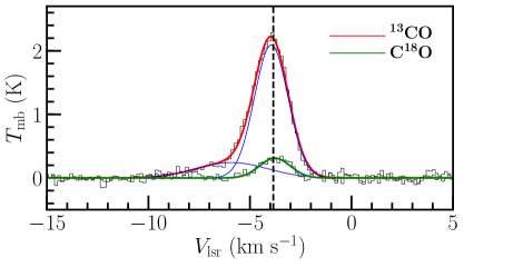
Figure 1: Average spectra of ¹³CO, and C¹⁸O (2-1) over the G350.5 filamentary cloud. The black color stands for the observed spectrum. The red line is the Gaussian fitting to the spectrum of ¹³CO, which is a sum of the two Gaussian components (blue lines), the weak-emission one from $-9.0$ to $5.7$ km s^-1, and the major one from $-5.7$ to $-2$ km s^-1. The green line is the single-component Gaussian fitting to the spectrum of C¹⁸O, which matches the major component of the ¹³CO spectrum. The vertical dashed black line represents a systematic velocity of $-3.9$ km s^-1.

Before addressing the kinematic structure of G350.5, we first describe the spatial distribution of molecular emission. Figure 1 presents the average spectra of ¹³CO, and C¹⁸O (2-1) over the whole G350.5 system. The ¹³CO profile has two velocity components, one from $-9.0$ to $5.7$ km s^-1 (hereafter weak-emission component) and the other from $-5.7$ to $-2$ km s^-1 (hereafter major component); C¹⁸O has a single-peak profile corresponding to the major component of ¹³CO. The systemic velocity is determined to be $-3.9$ km s^-1 from the average spectrum of C¹⁸O (2-1).

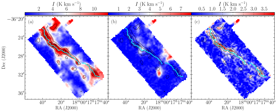
Figure 2: (a–b:) Velocity-integrated intensity maps of the two velocity components of ¹³CO (2-1) toward G350.5, the major one from $-5.7$ to $-2$ km s^-1, and the weak-emission one from $-9$ to $-5.7$ km s^-1. (c:) Velocity-integrated intensity of C¹⁸O (2-1), integrated over $-7$ to $-1$ km s^-1. The pixel size of the three maps is reduced to 7$\arcsec$, a quarter of the beam size, for a better visualization. The cyan curves in all panels represent the spines of the two discontinuous filaments as identified in Paper I and the black contours stand for the $N_{\rm H_{2}}$ column density (see Paper I), starting from $1.8\times 10^{22}$ cm^-2 with a step of $0.6\times 10^{22}$ cm^-2 ($\sigma=0.04\times 10^{22}$ cm^-2).

Figure 2 shows the velocity-integrated intensity maps of ¹³CO, and C¹⁸O (2-1). The spatial distribution of the major component of ¹³CO (see Fig. 2a) matches the column density ($N_{\mathrm{H_{2}}}$) distribution (black contours, derived from Herschel data in Paper I through the pixel-wise spectral energy distribution fitting, e.g., Liu, et al. 2016, 2017), showing two discontinuous filaments as indicated by the two cyan curves. In addition, some small-scale structures (i.e., filament ‘branches’) stretch perpendicular to the main structure of the cloud G350.5, which coincide with the perpendicular dust striations surrounding the filament as observed in Herschel continuum images (see Paper I). Emission of the major component of ¹³CO (2-1) has a C¹⁸O counterpart (in Fig. 2c), but the latter is more narrowly distributed than the former. In contrast, the weak-emission component of ¹³CO (2-1) in Fig. 2b has no detectable C¹⁸O counterpart. However, it can be seen that the two components of ¹³CO are indeed associated with each other. In the south and center of the filament, the two most prominent clumps in the intensity map of the ¹³CO weak-emission component can also be found in that of the major component. This is supportive of the association between the weak-emission and major components.

3.2 Velocity field along the filament

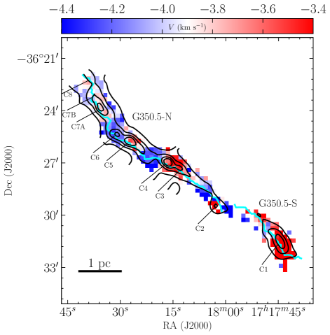
Figure 3: Velocity centroid map of C¹⁸O (2-1) for the filamentary cloud G350.5. Only the main filament is shown because of sufficient detection of C¹⁸O (2-1) therein. The pixel size of the map is 14$\arcsec$, half of the beam size, as recommended by the APEX observatory. All pixels correspond to detection greater than $3\sigma$ (i.e., $\sigma=0.4$ K km s^-1). The red and blue color scales can be regarded as the red and blue-shifted velocities with respect to the systematic velocity $-3.9$ km s^-1. A large-scale periodic velocity fluctuation appears almost along the main structure. The black contours represent the $N_{\rm H_{2}}$ column density, starting from $1.8\times 10^{22}$ cm^-2 with a step of $0.6\times 10^{22}$ cm^-2. The dense cores identified in Paper I are also labelled as C1–C8.

To investigate the large-scale kinematics, we show the velocity centroid map of C¹⁸O (2-1) of the cloud G350.5 in Fig. 3. Velocity information is shown only in the main structure of the filament, beyond which C¹⁸O (2-1) emission is too noisy ($<2\sigma$), overlaid with the $N_{\mathrm{H_{2}}}$ contours (Paper I) for comparison. Strikingly, a large-scale periodic velocity fluctuation appears along the main structure, which is $\sim 8$ pc long (Paper I). The nature of the large-scale and periodic signal suggests that the observed velocity fluctuation is real, otherwise, this periodicity will be hardly maintained on a large scale if it happens by chance. Specifically, the red and blue colors in Fig. 3 represent the red and blue-shifted velocities relative to the systemic velocity of $-3.9$ km s^-1. Comparing the $N_{\mathrm{H_{2}}}$ contours with the velocity centroid map, we find a spatial correspondence between the velocity extremes and the density enhancements for some dense cores (i.e., C2, C5, C6, C7a,b, and C8). The possible origins of this correspondence will be discussed further in Sect. 4. We do not present here the velocity centroid map of ¹³CO (2-1), which does not show the periodic fluctuation as in C¹⁸O (2-1) emission. Since ¹³CO tends to trace more extended emission than C¹⁸O, the velocity characteristics revealed by both species are not necessarily the same.

3.3 Velocity dispersion along the filament measured from both ¹³CO and C¹⁸O

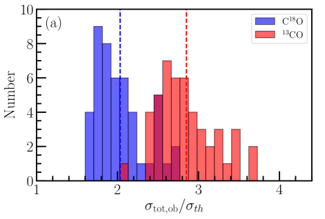
Figure 4: Histogram of the total velocity dispersion measured from both ¹³CO (red) and C¹⁸O (2-1) (blue) for G350.5. In panel (a) is the observed velocity dispersion. The mean values in the observed velocity dispersions measured from ¹³CO and C¹⁸O are $2.9\pm 0.4\,\sigma_{\rm th}$ (red dashed line), and $2.0\pm 0.3\,\sigma_{\rm th}$ (blue dashed line), respectively. In panel (b) is the opacity-corrected (intrinsic) velocity dispersion. The mean values are $2.1\pm 0.2\,\sigma_{\rm th}$ from ¹³CO (red dashed line), and $1.9\pm 0.3\,\sigma_{\rm th}$ from C¹⁸O (blue dashed line). The different distributions of the velocity dispersions of ¹³CO before and after the opacity correction demonstrate that the line opacity can cause the broadening of the intrinsic velocity dispersion. The intrinsic velocity dispersion distributions indicate that the overall turbulent motions of the filament G350.5 are supersonic (i.e., the 3D Mach number follows $M_{3D}>2$).

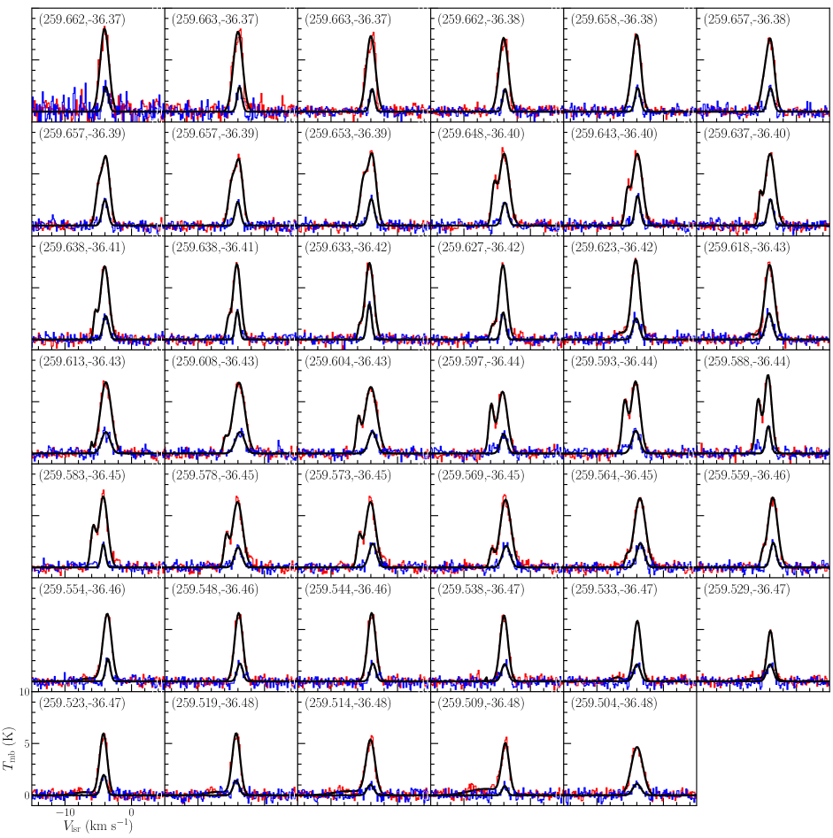
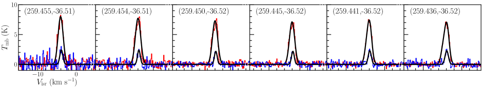
Figure 9: Gaussian-fitting results of both ¹³CO and C¹⁸O (2-1) for the selected 41 positions in G350.5-N (upper panel), and 6 positions in G350.5-S (bottom panel). The red and blue colors represent the observed spectra of ¹³CO  and C¹⁸O (2-1), respectively. The black stands for the fitting result.

The observed velocity dispersion ($\sigma_{\rm obs}$) is measured from both ¹³CO and C¹⁸O (2-1) in the main structure of the filament where both species are well-detected. In principle, $\sigma_{\rm obs}$ can be estimated from the second-order moment of the PPV data cube. However, this method will cause additional uncertainties due to the simple treatment of multiple-velocity components as one. To better estimate $\sigma_{\rm obs}$ especially from ¹³CO 2-1, we define 47 positions along the ridgeline of the filament, 41 in G350.5-N and 6 in G350.5-S. Neighbour positions are separated by one pixel, half of the beam size of both ¹³CO and C¹⁸O maps. $\sigma_{\rm obs}$ is then obtained from the Gaussian fitting to the spectra of both ¹³CO, and C¹⁸O (2-1) at the selected 47 positions. The fitting plots are shown in Fig. 9.

The velocity dispersion combines the contributions from both thermal and non-thermal gas motions in turbulent clouds. However, their contributions can be overestimated due to the line broadening by optical depth. Such overestimate can be expressed analytically as a function of the optical depth (Phillips et al., 1979):

$$\sigma_{\rm obs}=\frac{1}{\sqrt{ln2}}\left[ln\left(\frac{\tau}{ln\left(\frac{2}{e^{-\tau}+1}\right)}\right)\right]^{1/2}\sigma_{\rm int},$$ (1)

where $\sigma_{\rm int}$ is the intrinsic velocity dispersion unaffected by optical depth $\tau$ (see Appendix A). For comparison, we calculate the gas dispersions (i.e., non-thermal dispersion $\sigma_{\rm NT}$, and the total dispersion $\sigma_{\rm tot}$) based on the observed, and intrinsic velocity dispersions measured from both ¹³CO and C¹⁸O, respectively, as follows:

$$\begin{array}[]{rrr}\sigma_{\rm NT}=\sqrt{\sigma_{\rm obs/int}^{2}-\frac{kT_{\rm k}}{m}},\\ \sigma_{\rm th}=\sqrt{\frac{kT_{\rm k}}{\mu_{p}m_{\rm H}}},\\ \sigma_{\rm tot}=\sqrt{\sigma_{\rm NT}^{2}+\sigma_{\rm th}^{2}},\\ \end{array}$$ (2)

where $\sigma_{\rm obs/int}$ can be replaced either with $\sigma_{\rm obs}$ or with $\sigma_{\rm int}$ (see Eq. 1), $k$ is Boltzmann’s constant, $T_{\rm k}$ is the gas kinetic temperature, $m$ is the mass of the two species, $m_{\rm H}$ is the mass of atomic hydrogen, and $\mu_{p}=2.33$ is the mean molecular weight per free particle for an abundance ratio $N(H)/N(He)=10$ and a negligible admixture of metals (e.g., Kauffmann et al. 2008). The gas kinetic temperature here was assumed to be equal to the average dust temperature ($T_{\rm d}\sim 18\,K$) of the filament instead of the excitation temperature of each species since the latter is found to be $\sim 6$ K on average lower than the former, indicating that the two species might not be fully thermalized in the filament (see Appendix B for the calculation of the excitation temperature). The assumed $T_{\rm k}$ gives rise to the thermal sound speed of molecular gas $\sigma_{\rm th}\sim 0.25$ km s^-1.

Figure 4 presents the histograms of both the observed ($\sigma_{\rm tot,obs}$ in panel a) and intrinsic ($\sigma_{\rm tot,int}$ in panel b) total dispersions of gas for the entire filament represented by 41 positions in G350.5-N and 6 in G350.5-S. The intrinsic gas dispersion is overall smaller than the observed one without the optical-depth correction, indicating that the optical depth correction is important, especially for ¹³CO. In view of this, we analyse only the intrinsic gas dispersion (in Fig. 4b) in what follows. The average total dispersions are $2.1\pm 0.2\,\sigma_{\rm th}$, and $1.9\pm 0.3\,\sigma_{\rm th}$, measured from ¹³CO, and C¹⁸O, respectively. These values indicate that the filament G350.5 as a whole is supersonic with a mach number of $M_{3D}>2$ (see Fig. 4b), where the 3D Mach number is $M_{3D}=\sqrt{3}\sigma_{\rm NT,int}/\sigma_{\rm th}$ given the 1D measurement $\sigma_{\rm NT,int}$, and assuming isotropic turbulence in three dimensions (e.g., Kainulainen & Federrath, 2017).

3.4 Virial analysis along the filament

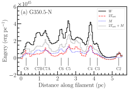
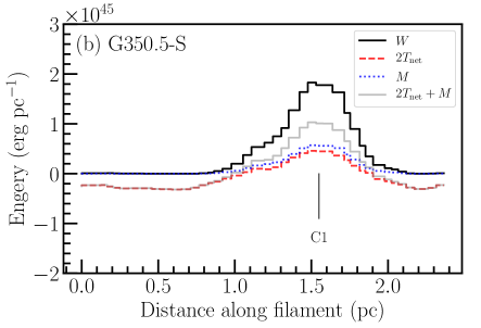
Figure 5: Virial analysis through the comparisons between turbulent ($T$), magnetic energies ($M$) and gravitational potential ($W$) for G350.5-N (in panel a), and for G350.5-S (in panel b). Several peaks are related to dense cores (also see Fig. 3) as indicated by vertical lines. The comparison shows that the gravity dominates over both turbulence and magnetic fields, and is a major driver to the global fragmentation of G350.5 from clouds to dense cores.

The complex interactions between turbulence, gravity and magnetic fields happen everywhere in molecular clouds and regulate star formation therein. We can describe these interactions through the virial theorem. According to Fiege & Pudritz (2000a), the virial equation of self-gravitating, magnetized turbulent filamentary clouds can be written in the form:

$$2T_{\rm net}+W+M=0.$$ (3)

Therefore, the virial equilibrium of the clouds depends on the competition between the net kinetic energy ($T_{\rm net}$), magnetic energy ($M$), and gravitational potential ($W$). $T_{\rm net}$ accounts for the difference between the internal ($T_{\rm int}$) and external ($T_{\rm ext}$) turbulent energy, assuming that molecular clouds are confined by the external pressure rather than completely isolated. Note that all energies here are measured per unit length.

The internal kinetic energy $T_{\rm int}$ is calculated as:

$$T_{\rm int}=\frac{1}{2}\ M_{\rm line}\ \sigma^{2}_{\rm tot,int},$$ (4)

where $M_{\rm line}$ is the line mass along the filament, which can be obtained in Fig. 3 of Paper I. While $\sigma_{\rm tot,int}$ measured from ¹³CO  and C¹⁸O (2-1) are similar, the one from ¹³CO (2-1) was finally adopted in the calculation since ¹³CO emission tends to trace larger-scale gas. The external turbulent energy $T_{\rm ext}$ can be expressed as a function of the external pressure $P_{\rm ext}$:

$$T_{\rm ext}={\it k}P_{\rm ext}\ \pi R_{\rm fil}^{2},$$ (5)

where k is the Boltzmann constant and $R_{\rm fil}$ is the filament radius, $\sim 0.5$ pc as measured in Paper I. A conservative value of $P_{\rm ext}=5\times 10^{4}$ K cm^-3 is assumed, which is in the range between $10^{4}$ K cm^-3 for the general ISM (Chromey, Elmegreen & Elmegreen, 1989) and $10^{5}$ K cm^-3 for several molecular clouds associated with HI complexes (Boulares & Cox, 1990).

The gravitational potential energy $W$ is derived from the line mass of the filament:

$$W=-M_{\rm line}^{2}G,$$ (6)

where $G$ is the gravitational constant. The magnetic energy $M$ is written as:

$$M=\frac{B^{2}}{2\mu_{0}}\pi R_{\rm fil}^{2},$$ (7)

where $B$ is the magnetic field strength and ${\mu_{0}}$ is the permeability of free space. $B$ is estimated following the empirical linear relationship between the field strength and gas column density. This relationship was summarized by Crutcher (2012) from Zeeman measurements in the form:

$$B=C\times N_{H}\,10^{-21}\,\mu G,$$ (8)

where $C$ is a constant, and $N_{\rm H}$ is the column density of atomic hydrogen gas. This constant was given to be 3.8 by Crutcher (2012) under the assumption of magnetic critical condition and a spherical shape of clouds, and improved to be 1.9 by Li et al. (2014) assuming a sheet-like shape. The mean column density of the cloud G350.5, $N_{\rm H_{2}}=8\times 10^{21}$ cm^-2 (Paper I), indicates an average B-field of $16$ $\mu$G. Even though this estimate of the B-field strength is very indirect, it can give us some insight into the role of the B-field versus gravity (see below).

Figure 5 presents the comparison between turbulent ($T$), gravitational ($W$) and magnetic ($M$) energies per unit length along the main structure of the two filaments G350.5-N, and G350.5-S. It can be seen that $W$ (black curve) is greater than the sum of $T_{\rm net}$ and $M$ (light grey curve) along the main structure of both G350.5-N and G350.5-S with respective mean ratios of $W/(T_{\rm net}+M)=2.0\pm 1.6$, and $2.5\pm 1.8$. This trend is in particular evident for the dense cores which correspond to the peaks in the distributions (see Fig. 5). This suggests that gravity dominates over both turbulence and magnetic fields, and is a major driver to the global fragmentation of G350.5 from clouds to dense cores. This is consistent with our previous analysis (Paper I) showing that G350.5 could have undergone radial collapse and fragmentation into distinct small-scale dense cores. Moreover, one can see that only turbulence without the aid of the B-field is not able to counteract gravity, suggesting the critical role of B-field in regulating molecular clouds against gravity. This is in agreement with existing observations showing that magnetic fields are important in filamentary clouds (e.g., Li et al., 2013, 2014, 2015; Stutz & Gould, 2016; Contreras et al., 2016). Future more accurate B-field strength measurements will provide direct constraints on the role of the magnetic fields in G350.5.

4 Discussion: Large-scale velocity oscillations along the filament

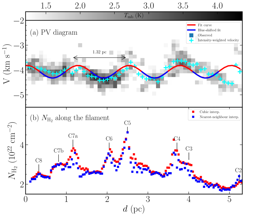
Figure 6: (a-b:) Velocity and column density distributions extracted along the spine of the filament G350.5-N. (a): Position-velocity diagram of C¹⁸O (2-1). The detections greater than $3\sigma$ ($\sigma=0.42$ K) are shown in grey-scale within the velocity channels from $-5.0$ to $-2.5$ km s^-1. The cyan crosses are the weighted average velocities by brightness temperatures, and fitted with a sine function with a wavelength of $\sim 1.3$ pc and an amplitude of $\sim 0.12$ km s^-1. Literally, the blue color curves stand for the blue-shifted velocities with respect to the systematic velocity of $-3.9$ km s^-1, and the red ones for the red-shifted velocities. (b:) Density distribution. Density peaks related to dense cores are indicated, i.e., C2 to C8, which are extracted from Fig. 3. The velocity and column density distributions do not show a good one-to-one correspondence between one another.

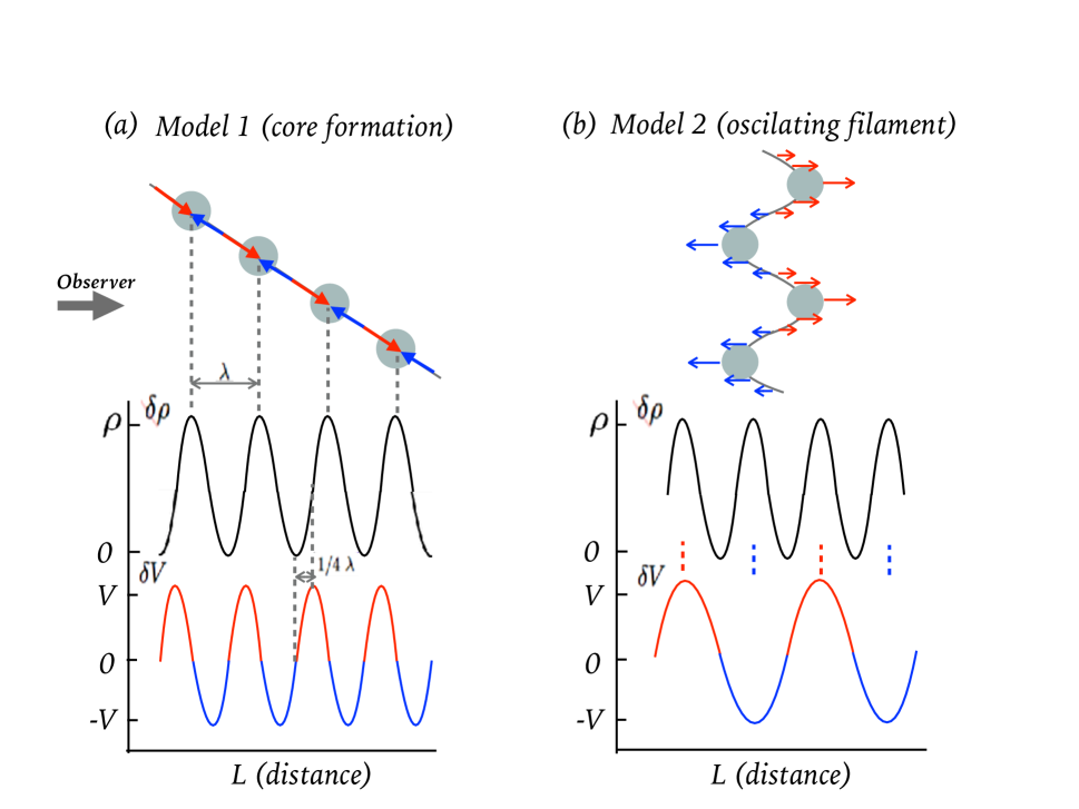
Figure 7: (a:) schematic representation of GI-driven core formation along a filament, which is adapted from Fig. 12 of Hacar & Tafalla (2011). Due to GI, the motions of core-forming gas converge towards the core centers where the density enhances but the relative motions become static with respect to the systematic velocity. In this scenario, assuming that both density ($\delta\rho$) and velocity ($\delta V$) follow sinusoidal distributions, a $\lambda/4$ phase shift between them would be expected. (b): schematic representation of a physical oscillating filament (e.g., induced by an MHD wave). The filament moves toward and away from an observer. In this scenario, the correspondence between the velocity extremes (i.e., red/blue-shifted velocities) and the density enhancements is expected if the filament (density) oscillates sinusoidally. The red and blue colors indicate the red, and blue-shifted velocities (motions) with respect to an observer. Note that the physical intensities of $\delta\rho$ and $\delta V$ are ignored in the schematic demonstration.

As mentioned in Sect. 3.2, a large-scale periodic velocity oscillation is found along the entire filament. This oscillation feature may be related to kinematics of either core formation or a large-scale oscillation (e.g., wave-like perturbations triggered by material accretion flows onto the filament or a standing wave Stutz, Gonzalez-Lobos, & Gould (2018)). In what follows, we will make an attempt to investigate the nature of the observed large-scale velocity oscillation in G350.5-N. Since G350.5-S is disconnected to G350.5-N in Fig. 3 and G350.5-S itself has insufficient detection in the diffuse region, the nature of the velocity field of G350.5-S requires detailed investigation with sensitive and higher-resolution observations. To better visualize the velocity oscillation along G350.5-N, we make the position-velocity (PV) diagram shown in Fig. 6a. The color scale is the main-beam temperature with at least $3\sigma$ ($\sigma=0.42$ K) detection within $-5.0$ to $-2.5$ km s^-1.

To highlight the velocity fluctuation feature, we calculate the average velocities weighted by the main-beam temperature, as shown in cyan crosses. In Fig. 6a, the velocity oscillation behaves periodically along the filament. Particularly, it can be fit with a sine function with a wavelength of $\sim 1.3$ pc and an amplitude of $\sim 0.12$ km s^-1.

4.1 Core formation through longitudinal gravitational instability?

In Paper I, nine identified cores are found to be distributed almost periodically along the entire filamentary cloud G350.5 and the average projected separations between them are measured to be $\sim 0.9$ pc. This separation is consistent with the prediction ($\sim 1.1$ pc in Paper I) by the “sausage” (gravitational) instability (Chandrasekhar & Fermi, 1953; Nagasawa, 1987), and comparable to the wavelength of the periodic velocity signature ($\sim 1.32$ pc, see above) inferred from the periodic velocity distribution as well. Therefore, the periodic velocity fluctuation may be associated with the kinematics of filament fragmentation into cores through gravitational instability (GI hereafter).

Actually, this periodic-type velocity fluctuation was already predicted in the analytic models dedicated to GI-induced core formation in a uniform, incompressible filament threaded by a purely poloidal magnetic field (e.g., Chandrasekhar & Fermi, 1953). In simulations, the GI is generally represented with redistributions of the gas in the filament via motions that have a dominant velocity component parallel to the cylinder axis due to longitudinal gravitational contraction at least during the first stages of evolution (e.g., Nakamura, Hanawa, & Nakano, 1993; Fiege & Pudritz, 2000b). The gas redistribution processes can be summarized in the schematic model of core formation as seen in Fig. 7a, where the motions of core-forming gas converge towards the core center along the filament, leading to the density enhancements peaking at a position of vanishing velocity. Assuming that both density and velocity perturbations (oscillations) are sinusoidal (periodic), a $\lambda/4$ shift between them can be expected (Hacar & Tafalla 2011 for more details). The similar pattern of velocity oscillation and its association with the density distribution have been reported in Taurus/L1517 (Hacar & Tafalla, 2011).

Comparing with the scenario of GI-induced core formation models, we do not observe a $\lambda/4$ ($\sim 0.33$ pc) phase shift between the velocity and density distributions (see Fig. 6). In addition, the predicted vanishing of velocity (see above) is not observed in most of the density enhancements cores (i.e., C2, C5, C6, C7a,b, and C8), and instead the velocity extremes coincide spatially with the density enhancements. Note that the above-mentioned models are rather idealised, and only designed for a straight filament. For example, if a filament were randomly kinked/curved on small scales, neither the systematic phase shift between the velocity and density distributions or the vanishing of velocity at the position of cores would be expected in the core formation process (see scenario 1 in Fig. 12 of Henshaw et al. 2014). However, we believe that the possibility of a randomly kinked structure is very low in G350.5-N since (random) small-scale kinks would not maintain a large-scale coherent, periodic oscillation. On the other hand, a regular but oscillating geometry driven by some physical mechanism could be possible (e.g., Gritschneder, Heigl, & Burkert 2017, see model 2 in Fig. 7, and Sect. 4.2 for more discussions).

Moreover, upon inspection of Fig. 3, we can group all dense cores into six main mass-accumulation clumps, i.e., C1 [red], C2 [red], C3+4 [red], C5+6 [red+blue], C7a+b [red+blue], and C8 [red]. They are almost periodically separated, which is demonstrated to be a result of filament fragmentation through GI (see above, and Paper I). Three of these clumps might have undergone further fragmentation due to GI or Jeans collapse (e.g., Kainulainen et al., 2017), leading to the observed multiplicity (i.e., from clumps to cores; C3+4 to C3 and C4, C5+6 to C5 and C6, and C7a+b to C7a and C7b). Such clump-scale fragmentation may influence the small-scale (inter-core) velocity distribution within the clumps. As a result, red and blue-shifted velocities would be expected on either side of dense cores in a straight filament. Assuming that G350.5-N is straight to some extent (see above), no red and blue-shifted velocities appearing on either side of the dense cores within two of the three clumps (i.e., C5+6, and C7a+b), therefore, imply that the clump-scale fragmentation (if any) would not significantly affect the large-scale periodic velocity pattern.

In addition, the average amplitude of the velocity oscillations is measured to be $\sim 0.12$ km s^-1. This value is around three times greater than that observed in Taurus/L1517 (Hacar & Tafalla, 2011). This difference could depend on the mass of dense cores and the inclination of the filament. Actually, the average mass of dense cores in G350.5-N is $\sim 20$ $M_{\odot}$, around 10 times higher than that in Taurus/L1517. Assuming free-fall gas accretion onto dense cores along the filament, we roughly calculate the infall velocity via the relation $V_{\rm infall}=\sqrt{GM*{\rm cos}\theta/r}$, where G is the gravitational constant, $r$ is the radius within which gas flows onto dense cores, adopted to be $1/4\lambda$ (0.33 pc), and $\theta$ is the inclination angle of the filament with respect to the line of sight. As a result, the average mass $\sim 20$ $M_{\odot}$ yields $V_{\rm infall}=\sim 0.5$ km s^-1 for $\theta=0\degr$, and $\sim 0.4$ km s^-1 for $\theta=45\degr$, both of which are around 4 times greater than the amplitude of the velocity oscillation in G350.5-N. Note that these infall velocities should be overestimated to be the accretion velocity of gas onto dense cores since neither gas accretion is purely free-fall in reality nor the infall commences at an infinite radius as assumed in the above equation (e.g., Vázquez-Semadeni et al. 2019). Keeping this uncertainty in mind, and given core formation through GI being at work in G350.5 (see above, and Paper I), we suggest that core-forming gas motions induced by GI could contribute in part to the observed velocity oscillation. However, another mechanism (e.g., see Model 2 in Fig. 7, and Sect. 4.2) is still required to explain the discrepancy between the observations and idealized GI-induced core-formation models, i.e., the lack of a constant phase shift observed between the velocity and density distributions.

4.2 Large-scale MHD-transverse wave propagating along the filament?

As mentioned in Sect. 4.1, there could be a mechanism responsible for the observed relation between the velocity and density distributions (see Fig. 6). We conjecture that this mechanism might be the MHD-transverse wave propagating along the filament, which can also produce a periodic velocity oscillation. Actually, this mechanism was reported both in observations and in simulations (e.g., Nakamura & Li, 2008; Stutz & Gould, 2016). For example, combining both observed spatial and velocity undulations and the helical B-field measurements in the Orion integral-shaped filament (ISF), Stutz & Gould (2016) suggested that repeated propagation of transverse waves through the filament are progressively digesting the material that formerly connected Orion A and B into stars in discrete episodes. In three-dimensional MHD simulations of star formation in turbulent, magnetized clouds, including feedback from protostellar outflows, Nakamura & Li (2008) mentioned that stellar feedback like outflows can induce large-amplitude Alfvén waves, which perturb the field lines in the envelope that thread other parts of the condensed sheet. The large Alfvén speed in the diffuse envelope allows different parts of the sheet to interact with each other quickly. Such interaction can spring up global, magnetically mediated oscillations for the condensed material (Nakamura & Li, 2008). The appearance of a large-scale MHD-transverse wave along the filament is understandable as long as there is a poloidal component of B-field, which is expected with generally helical and other configurations of 3D magnetic fields (e.g., Heiles, 1997; Fiege & Pudritz, 2000a, b; Stutz & Gould, 2016; Schleicher & Stutz, 2018; Reissl et al., 2018)

In the filament G350.5-N, the driving source of the large-scale MHD-transverse wave could result from outflows of young stellar objects (Nakamura & Li, 2008). In addition, the gas accretion flows onto the filament (see Paper I) could be an additional driving source. In principle, a wave-like shape of spatial density distribution could be expected as observed in the Orion-A ISF (Stutz & Gould, 2016). However, it can not be recognized from Fig. 2. This could be because of projection effects. That is, the large-scale MHD-transverse wave oscillates toward and away from us (see model 2 in Fig. 7) while propagating along the filament. As a result, the filament is projected to be a rather straight morphology on the plane-of-sky but the periodic velocity oscillation can be observed to blue and red-shifted with respect to the systemic velocity.

To conclude, given the GI-induced core formation being at work in G350.5-N (see Sect. 4.1), we suggest that the observed periodic velocity oscillation may result from a combination of the core-forming gas motions induced by GI and a periodic physical oscillation driven by a MHD transverse wave. This combination can make $\lambda/4$ shift, as expected between the velocity and density distributions in the core-formation models (see Model 1 of Fig. 7), disappear due to the mixture of the two different motions. Instead, the wave could cause the correspondence between the velocity extremes and density enhancements (see Fig. 6) if the wave is stronger than the core-forming gas motions in velocity amplitude. Despite of no definitive interpretation, it is worthwhile to test the possibility of the large-scale transverse wave being at work in G350.5-N. Therefore, we call for future high sensitivity/resolution Zeeman, and dust polarization measurements to infer the B-field strength and to constrain the field morphology (see above).

5 Conclusions

We have analysed the internal kinematics of the filament G350.5 with our observations of ¹³CO, and C¹⁸O (2-1) by APEX. ¹³CO emission reveals two clouds with different velocities. The major cloud G350.5 corresponds to $-5.7$ to $-2$ km s^-1 while the other one corresponds to $-9.0$ to $5.7$ km s^-1. Our analysis shows that the filament G350.5 as a whole is supersonic and gravitationally bound. In addition, we find a large-scale periodic velocity oscillation along the filament G350.5-N with a wavelength of $\sim 1.3$ pc and an amplitude of $\sim 0.12$ km s^-1. Comparing with the gravitational-instability induced core formation models, we suggest that the observed periodic velocity oscillation may result from a combination of the kinematics of gravitational instability-induced core formation and a periodic physical oscillation driven by a MHD transverse wave. To test the latter, future high sensitivity, and resolution Zeeman, and dust polarization measurements toward G350.5 are required to infer the B-field strength and to constrain the field morphology

Acknowledgments
We thank the anonymous referee for constructive comments that improved the quality of our paper. This work was in part sponsored by the Chinese Academy of Sciences (CAS), through a grant to the CAS South America Center for Astronomy (CASSACA) in Santiago, Chile. AS acknowledges funding through Fondecyt regular (project code 1180350), “Concurso Proyectos Internacionales de Investigación” (project code PII20150171), and Chilean Centro de Excelencia en Astrofísica y Tecnologías Afines (CATA) BASAL grant AFB-170002. J. Yuan is supported by the National Natural Science Foundation of China through grants 11503035, 11573036. This research made use of Astropy, a community-developed core Python package for Astronomy (Astropy Collaboration, 2018).

Appendix A Optical depth

Following the radiative transfer equations with an assumption of optically thin C¹⁸O (2-1) emission (e.g., Garden et al., 1991), we calculated the optical depth ($\tau$) of ¹³CO, and C¹⁸O (2-1) for the selected positions in the main structure of G350.5 as below:

$$\frac{T_{\rm mb}^{{{\rm{}^{13}CO}}}}{T_{\rm mb}^{{{\rm C^{18}O}}}}\approx\frac{1-e^{\tau_{13}}}{1-e^{\tau_{18}}}\approx\frac{1-e^{\tau_{13}}}{1-e^{\tau_{13}/R}},$$ (9)

where $T_{\rm mb}$ is the main-beam temperature for the two species, and the isotope ratio $R=[{\rm{}^{13}CO}]/[{\rm C^{18}O}]$ is adopted to be 7.7 following the derivation in Yuan et al. (2016). Instead of the weak-emission component of ¹³CO (2-1), its main velocity component matching the C¹⁸O (2-1) counterpart was taken into account in the practical calculations. With $\tau_{13}$ estimated, we can obtain $\tau_{18}$ via the relation $\tau_{18}=\tau_{13}/R$. The statistics of the estimated optical depths for both species is shown in Fig. 8. It can be seen that all of C¹⁸O (2-1) emission in the main structure of G350.5 are optically thin while ¹³CO (2-1) emission is optically thick with optical depths up to $4.6$.

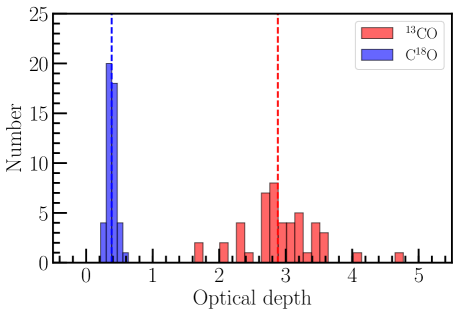
Figure 8: Histogram of the optical depth for ¹³CO (a) and C¹⁸O (b). The majority of C¹⁸O (2-1) emission appears to be optically thin while ¹³CO (2-1) emission suffers more optically thick effects.

Appendix B Excitation temperature

We further evaluated the excitation temperatures for the selected positions in the main structure of the filament following Liu et al. (2015):

$$\begin{array}[]{rrr}T_{\rm mb}=\frac{\mathrm{h}\nu}{\mathrm{k}}[\frac{1}{J_{\nu}(T_{\mathrm{ex}})}-\frac{1}{J_{\nu}(T_{\mathrm{bg}})}]$$[1-\mathrm{exp}(-\tau)]f,\end{array}$$ (10)

where $J_{\nu}$ is defined as $\frac{1}{\mathrm{exp}(\mathrm{h}\nu/\mathrm{k}T)-1}$, $T_{\rm mb}$ is the main-beam temperature, $T_{\mathrm{ex}}$ is the exciting temperature, and $T_{\mathrm{bg}}=2.73$ K is the cosmic background radiation; $\tau$ is the optical depth, the fraction of the telescope beam filled by emission $f$ is assumed to be 1, B and $\mu$ are the rotational constant and the permanent dipole moment of molecules respectively. Given the optical depth (in Sect. A) and $T_{\rm mb}^{{{\rm{}^{13}CO}}}$, we obtained the excitation temperature of ¹³CO (2-1) from Eq. 10. As a result, the average excitation temperature of ¹³CO (2-1) in the main structure of the filament is $12\pm 0.8$ K, which is $\sim 6$ K less than the corresponding average dust temperature there derived from the dust temperature map (Paper I). This difference may be related to non full thermalization of ¹³CO (2-1) in the main structure of G350.5.

Appendix C Gaussian fitting results

References

- (1)
- André et al. (2014) André P., Di Francesco J., Ward-Thompson D., Inutsuka S.-I., Pudritz R. E., Pineda J. E., 2014, prpl.conf, 27
- André et al. (2010) André P., et al., 2010, A&A, 518, L102
- Beuther et al. (2015) Beuther H., Ragan S. E., Johnston K., Henning T., Hacar A., Kainulainen J. T., 2015, A&A, 584, A67
- Boulares & Cox (1990) Boulares A., Cox D. P., 1990, ApJ, 365, 544
- Chandrasekhar & Fermi (1953) Chandrasekhar S., Fermi E., 1953, ApJ, 118, 116
- Chromey, Elmegreen & Elmegreen (1989) Chromey F. R., Elmegreen B. G., Elmegreen D. M., 1989, AJ, 98, 2203
- Contreras et al. (2016) Contreras Y., Garay G., Rathborne J. M., Sanhueza P., 2016, MNRAS, 456, 2041
- Crutcher (2012) Crutcher R. M., 2012, ARA&A, 50, 29
- Fiege & Pudritz (2000a) Fiege J. D., Pudritz R. E., 2000a, MNRAS, 311, 85
- Fiege & Pudritz (2000b) Fiege J. D., Pudritz R. E., 2000b, MNRAS, 311, 105
- Garden et al. (1991) Garden R. P., Hayashi M., Gatley I., Hasegawa T., Kaifu N., 1991, ApJ, 374, 540
- Güsten et al. (2006) Güsten R., Nyman L. Å., Schilke P., Menten K., Cesarsky C., Booth R., 2006, A&A, 454, L13
- Gritschneder, Heigl, & Burkert (2017) Gritschneder M., Heigl S., Burkert A., 2017, ApJ, 834, 202
- Hacar & Tafalla (2011) Hacar A., Tafalla M., 2011, A&A, 533, A34
- Hacar et al. (2018) Hacar A., Tafalla M., Forbrich J., Alves J., Meingast S., Grossschedl J., Teixeira P. S., 2018, A&A, 610, A77
- Hacar et al. (2017) Hacar A., Alves J., Tafalla M., Goicoechea J. R., 2017, A&A, 602, L2
- Heiles (1997) Heiles C., 1997, ApJS, 111, 245
- Henshaw, Longmore, & Kruijssen (2016) Henshaw J. D., Longmore S. N., Kruijssen J. M. D., 2016, MNRAS, 463, L122
- Henshaw et al. (2014) Henshaw J. D., Caselli P., Fontani F., Jiménez-Serra I., Tan J. C., 2014, MNRAS, 440, 2860
- Kainulainen et al. (2017) Kainulainen J., Stutz A. M., Stanke T., Abreu-Vicente J., Beuther H., Henning T., Johnston K. G., Megeath S. T., 2017, A&A, 600, A141
- Kainulainen & Federrath (2017) Kainulainen J., Federrath C., 2017, A&A, 608, L3
- Kauffmann et al. (2008) Kauffmann J., Bertoldi F., Bourke T. L., Evans N. J., II, Lee C. W., 2008, A&A, 487, 993
- Kirk et al. (2013) Kirk H., Myers P. C., Bourke T. L., Gutermuth R. A., Hedden A., Wilson G. W., 2013, ApJ, 766, 115
- Könyves & André (2015) Könyves V., André P., 2015, IAUGA, 22, 2250001
- Li et al. (2014) Li H.-B., Goodman A., Sridharan T. K., Houde M., Li Z.-Y., Novak G., Tang K. S., 2014, prpl.conf, 101
- Li et al. (2013) Li H.-b., Fang M., Henning T., Kainulainen J., 2013, MNRAS, 436, 3707
- Li et al. (2015) Li H.-B., et al., 2015, Natur, 520, 518
- Liu et al. (2015) Liu H.-L., Wu Y., Li J., Yuan J.-H., Liu T., Dong X., 2015, ApJ, 798, 30
- Liu, et al. (2017) Liu H.-L., et al., 2017, A&A, 602, A95
- Liu, et al. (2016) Liu H.-L., et al., 2016, ApJ, 818, 95
- Liu, Stutz, & Yuan (2018a) Liu H.-L., Stutz A., Yuan J.-H., 2018, MNRAS, 478, 2119
- Liu, et al. (2018b) Liu T., et al., 2018, ApJ, 859, 151
- Lu et al. (2018) Lu X., et al., 2018, ApJ, 855, 9
- Molinari et al. (2010) Molinari S., et al., 2010, A&A, 518, L100
- Nagasawa (1987) Nagasawa M., 1987, PThPh, 77, 635
- Nakamura, Hanawa, & Nakano (1993) Nakamura F., Hanawa T., Nakano T., 1993, PASJ, 45, 551
- Nakamura & Li (2008) Nakamura F., Li Z.-Y., 2008, ApJ, 687, 354
- Peretto et al. (2013) Peretto N., et al., 2013, A&A, 555, A112
- Peretto et al. (2014) Peretto N., et al., 2014, A&A, 561, A83
- Phillips et al. (1979) Phillips T. G., Huggins P. J., Wannier P. G., Scoville N. Z., 1979, ApJ, 231, 720
- Ragan et al. (2012) Ragan S., et al., 2012, A&A, 547, A49
- Reissl et al. (2018) Reissl S., Stutz A. M., Brauer R., Pellegrini E. W., Schleicher D. R. G., Klessen R. S., 2018, MNRAS, 481, 2507
- Schleicher & Stutz (2018) Schleicher D. R. G., Stutz A., 2018, MNRAS, 475, 121
- Schneider & Elmegreen (1979) Schneider S., Elmegreen B. G., 1979, ApJS, 41, 87
- Stutz & Kainulainen (2015) Stutz A. M., Kainulainen J., 2015, A&A, 577, L6
- Stutz (2018) Stutz A. M., 2018a, MNRAS, 473, 4890
- Stutz, Gonzalez-Lobos, & Gould (2018) Stutz A. M., Gonzalez-Lobos V. I., Gould A., 2018b, arXiv, arXiv:1807.11496
- Stutz & Gould (2016) Stutz A. M., Gould A., 2016, A&A, 590, A2
- Tackenberg et al. (2014) Tackenberg J., et al., 2014, A&A, 565, A101
- Tafalla & Hacar (2015) Tafalla M., Hacar A., 2015, A&A, 574, A104
- Vázquez-Semadeni et al. (2019) Vázquez-Semadeni E., Palau A., Ballesteros-Paredes J., Gómez G. C., Zamora-Avilés M., 2019, arXiv e-prints, arXiv:1903.11247
- Yuan et al. (2016) Yuan J., et al., 2016, ApJ, 820, 37
- Yuan, et al. (2018) Yuan J., et al., 2018, ApJ, 852, 12
- Williams et al. (2018) Williams G. M., Peretto N., Avison A., Duarte-Cabral A., Fuller G. A., 2018, A&A, 613, A11
- Wu et al. (2018) Wu G., Qiu K., Esimbek J., Zheng X., Henkel C., Li D., Han X., 2018, A&A, 616, A111