Learning phase transitions:comparing PCA and SVM

Abstract

A comparison of results from principal component analysis and support vector machine calculations is made for a variety of phase transitions in two-dimensional classical spin models.

1 Introduction

Machine learning methods are becoming more and more prevalent in physics research. One very active area of application is in the identification and characterization of phase transitions. Some examples of recent work include Refs. [1-8]. An attractive feature of machine learning techniques is that they can use the raw data from Monte Carlo simulations, for example, the spin configurations from a spin model, to infer the presence or nature of a phase transition without the a priori construction of an order parameter or other thermodynamic function.

Most recent work focuses on the two-dimensional Ising model. However, in Ref. [2] Hu et al. present a more comprehensive survey of principal component analysis (PCA) applied to Monte Carlo data for a variety of classical spin systems. PCA is an unsupervised method which identifies variables (principal components) whose behaviour as a function of simulation parameters can expose the presence of a phase transition. For example, Hu et al. show that for the Ising model and other phase transitions PCA identifies the magnetization as the leading principal component without the input of any domain knowledge. Furthermore, the pattern of principal components can be used to distinguish crossover behaviour from a genuine phase transition.

In Ref. [6, 7] support vector machines (SVM) were used to study the phase transition in the Ising model. SVM is a supervised algorithm which can be trained using Monte Carlo data to distinguish between the ordered and unordered phases of a spin system. The decision function calculated for spin configurations which interpolate between the training sets can be used as proxy for an order parameter. This was discussed in detail for the Ising model in Ref.[7] .

The purpose of this note is

• to extend the SVM analysis to some spin systems which were not considered in Ref. [7]

• to make a comparison between the results of PCA and SVM analyses.

Sections 2 and 3 contain brief reviews of PCA and SVM respectively, Results of analyses of Monte Carlo data for the Ising, Blume-Capel and Biquadratic-exchange spin-1 Ising models are presented Sect. 4. A summary is given in Sect. 5

2 Principal component analysis

The key feature of principal component analysis [9] is the decomposition of a data set, considered as a set of points in a large dimensional space, along directions that are ordered by maximal variance. For the present problem the data set will consist of an ensemble of spin configurations on an $L\times L$ square lattice computed over a range of a simulation parameter (temperature or a Hamiltonian model parameter). The data can be written in the form of a matrix $\mathbf{S}$ where each row $\mathbf{S}_{i}$ ($i=1...N)$ consists of the $n=L^{2}$ values of the spin in a configuration and N denotes the number of rows i.e., the number of spin configurations. The first step is to subtract from each column its average value, call the resulting matrix $\mathbf{X}$. Weight vectors $\mathbf{w}_{i}$($j=1...n$) that transform $\mathbf{X}$ into principal components are defined iteratively (see Ref. [2]) or equivalently determined from a singular value decomposition which entails the solution of the eigenvalue problem (see[9])

$$\mathbf{X}\mathbf{{}^{T}X\mathbf{w}_{j}=\lambda_{j}\mathbf{w}_{j}.}$$ (1)

The final result is the principal decomposition of $\mathbf{S}$ given by $\mathbf{P}=\mathbf{S}\mathbf{W}$ or in component form

$$p_{ij}=\mathbf{S}_{i}\cdot\mathbf{w}_{j}.$$ (2)

Hu et al. define quantified principal components

$$\left\langle\left|p_{j}\right|\right\rangle=\frac{1}{N^{\prime}}\sum_{i}\left|p_{ij}\right|$$ (3)

where the average is over a subset $N^{\prime}$ of the spin configurations which have same simulation parameter values.

Principal component analysis is completely non-parametric and is useful when the data have significant structure in a small number of directions, i.e., a small number of large eigenvalues in Eqn. (1). In the present work the implementation of PCA in scikit-learn [10] was used.

3 Support vector machines

The support vector machine is a supervised learning method that can be used for classification and regression. In the present work it will be used as a binary classifier. The SVM is trained to classify elements of a data set consisting of spin configurations calculated at two different points in the simulation parameter space. If the training data lie on different sides of a phase transition, the ability of the trained SVM to label spin configurations intermediate to the training sets maybe used to investigate the phase transition, for example, to determine the transition point in the model parameter space.

To illustrate the concept of the SVM consider the simplest case: points $\mathbf{x}$ in an n-dimensional space $\mathbb{R}^{n}$ with a set of such points that can be separated into two groups (conventionally labeled by $y=\pm$1) by a hyperplane. The points on each side of the hyperplane that are closest to it in perpendicular distance are the support vectors (see Sect. 1.4.7 in [11] or Fig. 2 in [7]). The equation for a separating hyperplane takes the form

$$\mathbf{w}\cdot\mathbf{x}-b=0.$$ (4)

Training the SVM involves finding $\mathbf{w}$ and $b$ which minimize $\left\|\mathbf{w}\right\|^{2}$ subject to $y_{i}(\mathbf{w}\cdot\mathbf{x_{i}}-b)\geq 1$ for all points i in the training set. Using the solution of this minimization problem the decision function for any point $\mathbf{x}$ is defined to be

$$d(\mathbf{x})=\mathbf{w}\cdot\mathbf{x}-b.$$ (5)

The sign of $d(\mathbf{x})$ then assigns an arbitrary point to one of the two groups.

In real applications a complete linear separation of the data is usually not possible. A generalization to a so-called dual formulation can be made which also allows for the incorporation of non-linear features [7]. The details are omitted here and we quote only the final form of the decision function that will be used in subsequent analyses (see [7])

$$d(\mathbf{x})=\frac{1}{L^{4}}\sum_{i=1}^{n_{SV}}y_{i}\alpha_{i}(\mathbf{x_{i}}\cdot\mathbf{x})^{2}+b$$ (6)

where $i$ labels the support vector found in training. This form corresponds to the use of a homogeneous quadratic kernel [7], a kernel found to be appropriate for the Ising model and used here also for other spin models. For this work training and calculation of the decision function was done using functions in svm module of scikit-learn [10, 11].

We will study the behaviour of spin systems as a function of a single parameter. Suppose that the training set consists of data calculated at parameter values $t_{1}$ and $t_{2}$ which may correspond to two different phases. The decision function serves as a measure of how well the SVM can associate data calculated for parameter values between $t_{1}$ and $t_{2}$ with the different phases and will be used as a proxy for an order parameter.

4 Results

4.1 Ising model

The two-dimensional Ising model is a useful testbed for methods of studying phase transitions since the exact solution is known [12, 13]. The Hamiltonian is

$$H=-J\sum_{\left\langle i,j\right\rangle}s_{i}s_{j},$$ (7)

with $s_{i}=\pm$1 and the sum is over nearest-neighbour sites. For positive $J$ there is a transition from an ordered (ferromagnetic) spin state to an unordered (paramagnetic) state at $T_{c}/J=2/ln(1+\sqrt{2}).$ Principal component analysis of the Ising model was presented in [2] and SVM was discussed in [6, 7] so here we show only a few results to set the stage for discussion of other models.

Spin configurations were generated using a Monte Carlo method for lattices $L$ = 64 with periodic boundary conditions at 19 values of the temperature. Data at temperatures (in units of $J$) $\mathrm{T}{}_{1}$ and $\mathrm{T}{}_{2}$ equal 1.0 and 4.0 respectively were used for training the SVM. Analysis was done for data at seventeen values of the temperature spanning the range 1.5 to 2.9. At each temperature 800 well separated spin configurations were obtained.

Quantities conventionally used in the analysis of spin models, the absolute magnetization

$$\left\langle\left|M\right|\right\rangle=\frac{1}{N^{\prime}}\sum_{\{s\}}\left(\nicefrac{{\left|\sum_{j}s_{j}\right|}}{{n}}\right),$$ (8)

the squared magnetization

$$\left\langle M^{2}\right\rangle,$$ (9)

and the susceptibility

$$\left\langle\chi\right\rangle=n\frac{\left\langle M^{2}\right\rangle-\left\langle\left|M\right|\right\rangle^{2}}{T}$$ (10)

were also computed as a function of temperature from the Monte Carlo data to compare with what PCA and SVM learned.

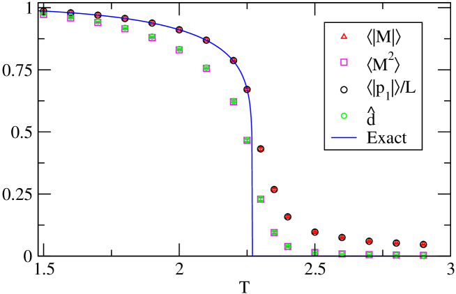
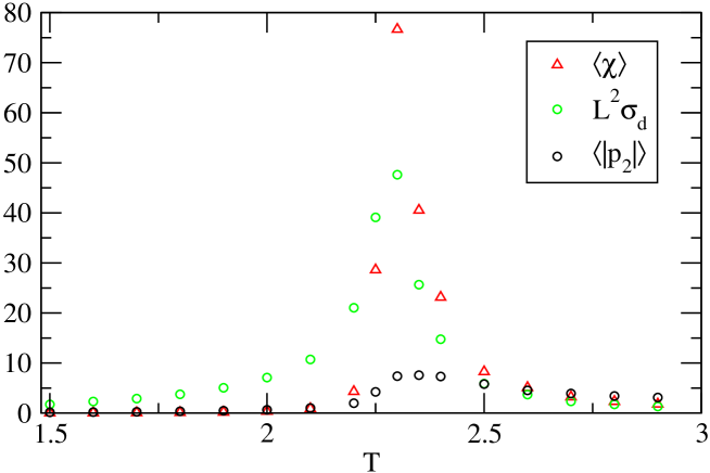
Figure 1: Summary of results for the Ising model on a lattice with $L$ = 64. The exact result for the magnetization [13] is also shown (solid line).

Figure 2: The scaled standard deviation of the SVM decision function $L^{2}\sigma_{d}$ and the quantified second principal component from PCA $\left\langle\left|p_{2}\right|\right\rangle$ compared to the susceptibility for the Ising model as a function of temperature.

Magnetization results are summarized in Fig. 2. The leading quantified principal component $\left\langle\left|p_{1}\right|\right\rangle$ tracks $\left\langle\left|M\right|\right\rangle$ essentially exactly. In other words, PCA picks out the magnetization as the most important feature of the data. To illustrate what SVM learns we define a modified decision function $\hat{d}$ by shifting and rescaling $d$ so that $\hat{d}$ is equal to the squared magnetization at the training points $T_{1}$ and$T_{2}$. Fig. 2 shows that the modified decision function reproduces the squared magnetization. As discussed in [6, 7] this is expected for the SVM with a quadratic kernel.

In the vicinity of a continuous phase transition fluctuations on all scales become important. This is reflected in simulations by an increase of susceptibility (proportional to the variance of the magnetization) in the transition region. It is suggested in [7] on the basis of dimensional analysis that the standard deviation of the decision function can also be used to identify the critical temperature. These quantities are shown in Fig. 2. To facilitate plotting, the standard error of $d$ (standard deviation/$\sqrt{N^{\prime}})$ is used. Both quantities show a sharp peaking in the region of the known critical temperature [12] $\approx$2.269. As noted in [2] the second quantified principal component from PCA $\left\langle\left|p_{2}\right|\right\rangle$ also peaks in the region of the critical temperature. However, this feature is not very prominent and probably not as useful for quantitative analysis as the information from SVM.

4.2 Blume-Capel model

The Blume-Capel model (BCM) [14, 15] is a generalization of the Ising model which allows for three spin values $s_{i}=\pm 1,0$. The Hamiltonian takes the form

$$H=-J\sum_{\left\langle i,j\right\rangle}s_{i}s_{j}+\Delta\sum_{i}s_{i}^{2}.$$ (11)

The parameter $\Delta$ controls the density of spin 0 sites. The transition from an ordered to an unordered spin state may be first or second order depending on the model parameters. There is a tricritical point at $(T/J,\Delta/J)$ = [0.609(4), 1.965(5)] [16].

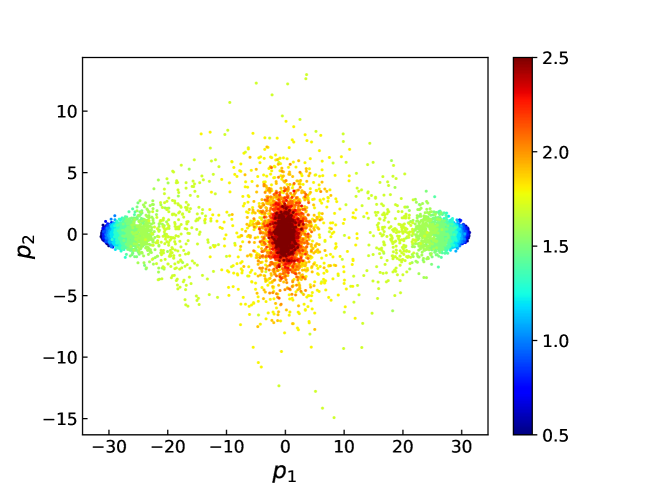
Figure 3: Scatter plot of the two leading principal components from PCA of the Blume-Capel model at $T$ = 1, $J$ = 1 and $\Delta$ the range 0.5 to 2.5.

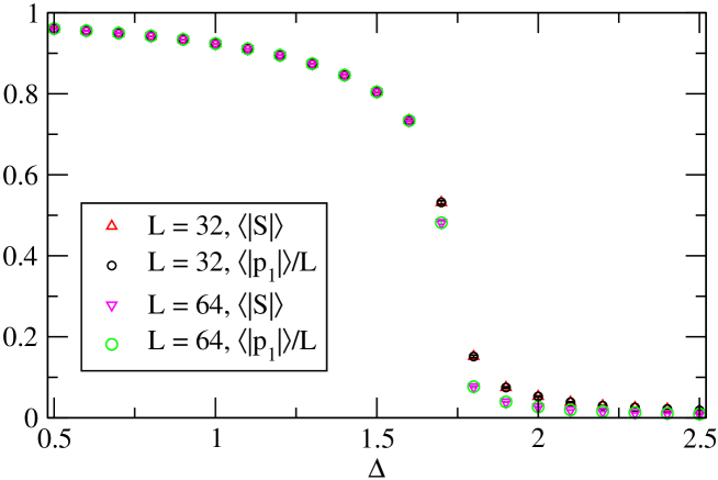
Figure 4: The quantified leading component from PCA compared to magnetization for the Blume-Capel model at $T$ = 1, $J$ = 1 as function $\Delta$.

Two different sets of model parameters were considered. The first set has fixed $T$ = 1 and $J$ =1 with varying $\Delta.$ Monte Carlo data were generated at $\Delta$ equal to 0.01 and 3.0 for SVM training and in the range 0.5 to 2.5 for analysis with 1000 configurations at each parameter point. Lattice sizes ranged from L = 32 to L = 256.

PCA was carried out for the L= 32 and L = 64 data. Fig. 3 shows the scatter plot of the first two principal components for L = 32 (compare to Fig. 5(b) in [2]). The clear separation into distinct regions is an indicator of a transition. The presence of two lobes at larger $|p_{1}|$ and small $p_{2}$ reflects the fact that there are two possible ordered ground states. As in the case of the Ising model PCA picks out the magnetization as the most prominent feature of the data which is encoded in $p_{1}.$ This is is illustrated in Fig. 4.

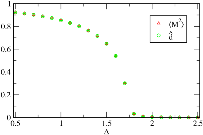
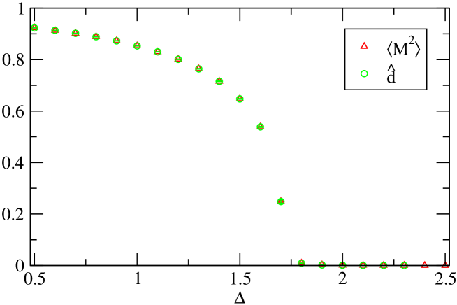
Figure 5: The modified decision function $\hat{d}$ from SVM compared to the squared magnetization for the Blume-Capel model at $T$ = 1, $J$ = 1 as function $\Delta$ on a lattice with $L$ = 32.

Figure 6: The modified decision function $\hat{d}$ from SVM compared to the squared magnetization for the Blume-Capel model at $T$ = 1, $J$ = 1 as function $\Delta$ on a lattice with $L$ = 64.

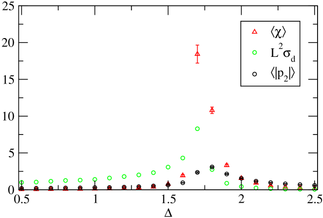
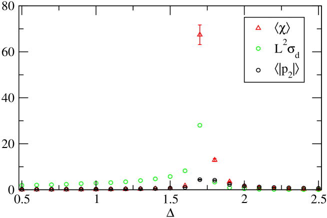
Figure 7: The scaled standard deviation of the SVM decision function $L^{2}\sigma_{d}$ and the quantified second principal component from PCA $\left\langle\left|p_{2}\right|\right\rangle$ compared to the susceptibility for the Blume-Capel model at $T$ = 1, $J$ = 1 as a function of $\Delta$ a lattice with $L$ = 32.

Figure 8: The scaled standard deviation of the SVM decision function $L^{2}\sigma_{d}$ and the quantified second principal component from PCA $\left\langle\left|p_{2}\right|\right\rangle$ compared to the susceptibility for the Blume-Capel model at $T$ = 1, $J$ = 1 as a function of $\Delta$ a lattice with $L$ = 64.

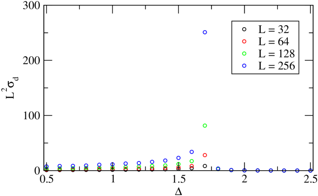
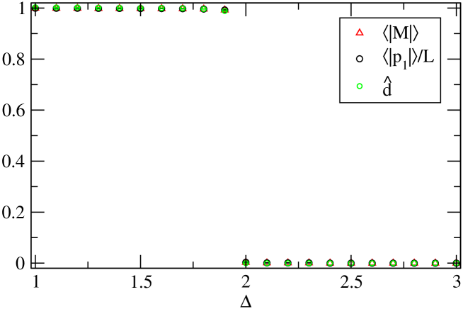
Figure 9: The scaled standard deviation of the SVM decision function $L^{2}\sigma_{d}$ for the Blume-Capel model at $T$ = 1, $J$ = 1 as a function of $\Delta$ on different size lattices.

Figure 10: The modified decision function $\hat{d}$ from SVM and the quantified first principal component from PCA $\left\langle\left|p_{1}\right|\right\rangle/L$ compared to the magnetization for the Blume-Capel model at $T$ = 0.4, $J$ = 1 as a function of $\Delta$ on a lattice with $L$ = 32.

SVM analysis was done for lattices from L = 32 to L = 256. The modified decision function $\hat{d}$ (pinned to squared magnetization at the training points) is compared to the squared magnetization for L = 32 and L = 64 data in Figs. 6 and 6. The quantified second principal component $\left\langle\left|p_{2}\right|\right\rangle$ from PCA and the scaled decision function standard deviation $L^{2}\sigma_{d}$ from SVM are compared to the spin susceptibility in Fig. 8 and 8. The sharp peaking in the vicinity of $\triangle$ = 1.7 is consistent with the critical $\Delta_{c}\approx$1.63 obtained in [17] at T = 1. The scaled decision function standard deviation $L^{2}\sigma_{d}$ for different lattice sizes is shown in Fig. 10. The increased peaking tending to a singularity as L increases is consistent with a second order phase transition.

The second model parameter set considered has T = 0.4 and $J$ =1. The results are shown in Fig. 10 for a lattice with L = 32. There is a first order phase transition at $\Delta_{c}\approx$1.996 [18] The outputs from PCA ($\left\langle\left|p_{1}\right|\right\rangle/L$ ) and SVM ($\hat{d}$ ) correctly identify this feature.

4.3 Biquadratic-exchange spin-1 Ising model

The biquadratic-exchange spin-1 Ising model (BSI) is a generalization studied in Ref. [2]. The Hamiltonian is

$$H=-J\sum_{\left\langle\left\langle i,j\right\rangle\right\rangle}s_{i}s_{j}+K\sum_{\left\langle i,j\right\rangle}s_{i}^{2}s_{j}^{2}$$ (12)

where $\left\langle\left\langle i,j\right\rangle\right\rangle$ denotes the sum over next-nearest-neighbour sites. At $J$ = 0 the ground state is disordered with two qualitatively different spin patterns connected by a crossover as a function of temperature. For $J\neq 0$ an ordered phase appears.

Analysis was done for two different model parameter sets. The first set has $K$= 1, $J$ = 0. Monte Carlo data were calculated for temperatures T from 0.08 to 2.60 on lattices from L =32 to L = 256. The magnetization is close to 0 at all temperatures. However, the spin pattern is different with some short-range order appearing at higher temperatures (see Fig. 1 in [2]).

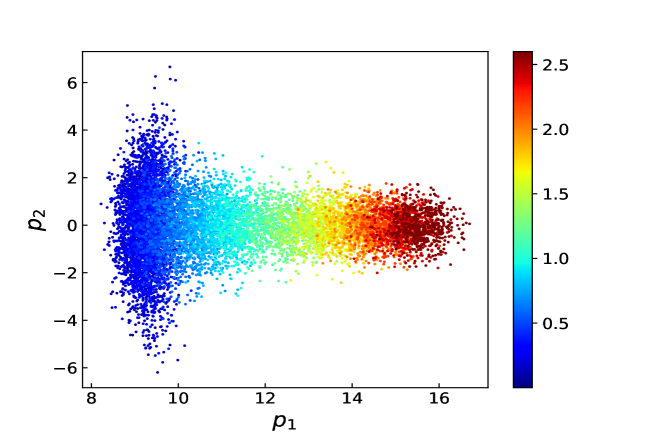
Figure 11: Scatter plot of the two leading principal components from PCA of the BSI model at $K$ =1, $J$ = 0 and temperature range 0.08 to 2.60 with squared spin input.

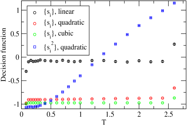
Figure 12: SVM decision function for the BSI model at $K$ =1, $J$ = 0 with different kernels using spin input.

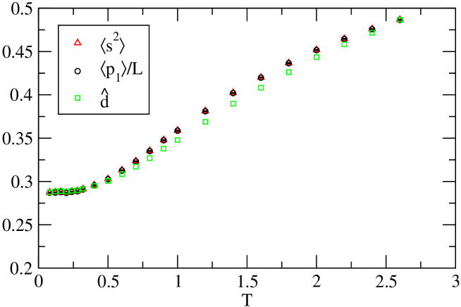
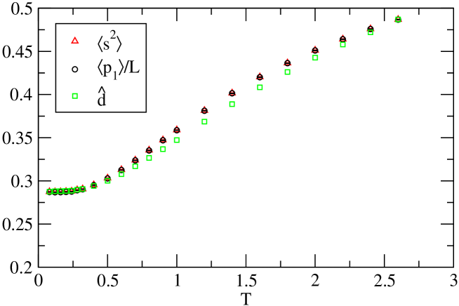
Figure 13: The modified decision function $\hat{d}$ from SVM and the quantified first principal component from PCA $\left\langle\left|p_{1}\right|\right\rangle/L$ compared to the expectation value of the squared spin $\left\langle s^{2}\right\rangle$ for the BSI model at $K$ = 1, $J$ = 0 as a function of $T$ on a lattice with $L$ = 32.

Figure 14: The modified decision function $\hat{d}$ from SVM and the quantified first principal component from PCA $\left\langle\left|p_{1}\right|\right\rangle/L$ compared to the expectation value of the squared spin $\left\langle s^{2}\right\rangle$ for the BSI model at $K$ = 1, $J$ = 0 as a function of $T$ on a lattice with $L$ = 64.

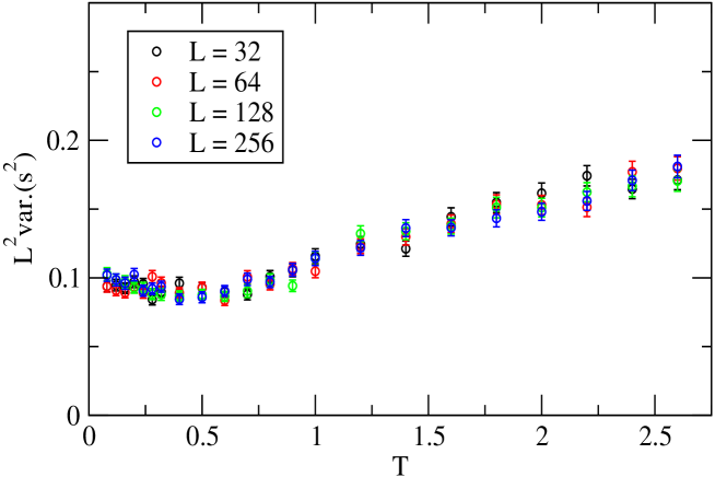
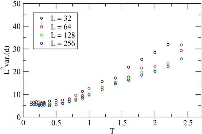
Figure 15: Variance of $s^{2}$ scaled by $L^{2}$ for the BSI model at $K$ = 1, $J$ = 0 as a function of $T$ on different size lattices.

Figure 16: Variance of the SVM decision function scaled by $L^{2}$ for the BSI model at $K$ = 1, $J$ = 0 as a function of $T$ on different size lattices.

As noted in [2] since PCA averages the spins over the configuration ensemble it fails to identify any prominent feature in the spin data and Hu et al. suggest the use of squared spin configurations $\{s_{i}^{2}\}$ in the analysis. Inputting these configurations gives Fig. 11 where one sees a dominant leading principal component which varies smoothly with temperature. The SVM also fails to classify correctly the spin configurations. Training with $T_{1}$= 0.08 and $T_{2}$ = 2.60 leads to test scores well below 1. Decision functions with spin input and different homogeneous polynomial kernels are shown in Fig. 12. Also shown is the decision function with squared spin input and a quadratic kernel. In this case the training data are classified correctly and the decision function interpolates smoothly between the training points.

Fig. 14 and 14 show the temperature dependence of the expectation of the squared spin

$$\left\langle s^{2}\right\rangle=\frac{1}{N^{\prime}}\sum_{\{s\}}\left(\nicefrac{{\sum_{j}s_{j}^{2}}}{{n}}\right)$$ (13)

along with output from PCA and SVM for L= 32 and L = 64. Comparison of these plots indicates little or no volume dependence. A question is whether or not the change in slope of the quantities plotted in Fig. 14 and 14 signals a phase transition. Hu et al. [2] suggest that the smooth behaviour of the leading principal component and the lack of distinct regions in Fig. 11 (in contrast to Fig.3 ) indicates a smooth crossover rather than a phase transition. A hallmark of a continuous phase transition is increased fluctuations that extend over the entire volume in the transition region (see Figs. 2 and 10). In Fig. 16 we plot $L^{2}$ times the variance of the squared spin as function of temperature for different volumes. No volume dependence or sharp peaking is observed. Fig. 16 shows $L^{2}$ times the variance of the decision function. The lack of sharp peaking indicates that the SVM analysis correctly identifies the change in the spin pattern as associated with a crossover rather than a phase transition.

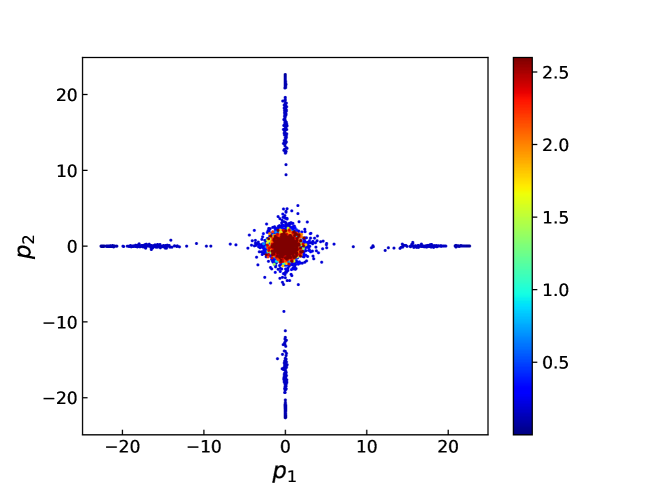
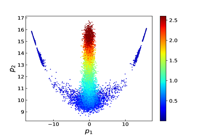
Figure 17: Scatter plot of the two leading principal components from PCA of the BSI model at $K$ =1, $J$ = 0.1 and temperature range 0.08 to 2.60 with spin input.

Figure 18: Scatter plot of the two leading principal components from PCA of the BSI model at $K$ =1, $J$ = 0.1 and temperature range 0.08 to 2.60 with squared spin input.

The second set of model parameters has $K$ = 1, $J$ = 0.1. At low temperatures an ordered phase with a checker board pattern of zero and nonzero spins appears (see Fig. 1 in [2]). PCA was carried out for spin simulation data in the temperature range 0.08 to 2.60. The scatter plot of the two leading principal components is shown in Fig. 18. The four arms show the presence of four possible ordered ground states at low temperature. Using the squared spin configurations $\{s_{i}^{2}\}$ as input the resulting $p_{1}$ versus $p_{2}$ correlation is given in Fig. 18. The interpretation of the principal components is not as obvious here as it was for the Ising or Blume-Capel model. Fig. 19 shows that with squared spin input the second quantified principal component reproduces the expectation value $\left\langle s^{2}\right\rangle.$

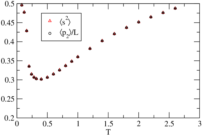
Figure 19: The quantified second principal component from PCA $\left\langle\left|p_{2}\right|\right\rangle/L$ compared to the expectation value of the squared spin $\left\langle s^{2}\right\rangle$ for the BSI model at $K$ = 1, $J$ = 0.1 as a function of $T$ on a lattice with $L$ = 32.

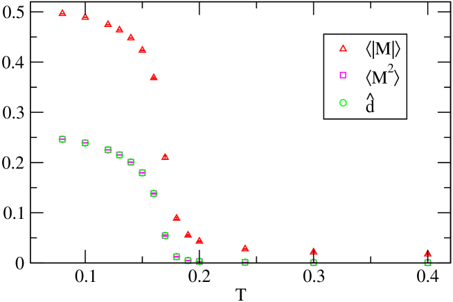
Figure 20: The modified decision function $\hat{d}$ from SVM compared to magnetization and squared magnetization for the BSI model at $K$ = 1, $J$ = 0.1 as a function of $T$ on a lattice with $L$ = 32.

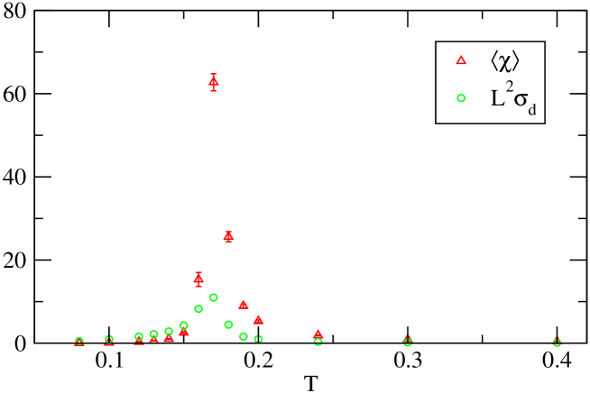
Figure 21: The scaled standard deviation of the SVM decision function $L^{2}\sigma_{d}$ compared to the susceptibility for the BSI model at $K$ = 1, $J$ = 0.1 as a function of $T$ on a lattice with $L$ = 32.

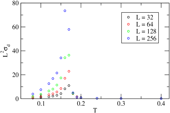
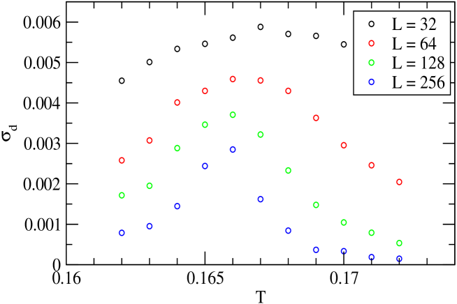
Figure 22: The scaled standard deviation of the SVM decision function $L^{2}\sigma_{d}$ for the BSI model at $K$ = 1, $J$ = 0.1 as a function of $T$ on different size lattices.

Figure 23: Standard deviation of the decision function versus temperature in the transition region for the BSI model at $K$ = 1, $J$ = 0.1 on different size lattices..

SVM analysis was done using spin configuration input with $T_{1}$= 0.08 and $T_{2}$ = 0.60 for training. The results for the modified decision function along with magnetization and squared magnetization are plotted in Fig. 20 for a lattice with L = 32. As with other models the modified decision function tracks the squared magnetization. The scaled standard deviation of the decision function as function of temperature is compared with the susceptibility $\left\langle\chi\right\rangle$ in Fig. 21. The peaking is indicative of a phase transition in the region $T$ = 1.7. To verify that there is a phase transition and to do a quantitative analysis volume dependence has to be examined. Fig. 23 shows the lattice size dependence of $L^{2}\sigma_{d}$ for lattices up to $L$ = 256.

To determine the critical temperature we use $L^{2}\sigma_{d}$ as proxy for the susceptibility and estimated the temperature of the peak position of this quantity for different volumes. Call this $T_{c}(L).$ Then $T_{c}(L)$ extrapolated to infinite volume gives $T_{c}.$ To get the peak position Monte Carlo data with 4000 configurations per temperature were generated for a fine scan with 0.162$\leq T\leq$0.172. The error in the decision function trained with $T_{1}$= 0.08 and $T_{2}$ = 0.60 is plotted in Fig. 23. The estimated peak values $T_{c}(L)$ along with an extrapolation $T_{c}+c/L$ are shown in Fig. 24. The inferred critical temperature is 0.1655(5), slightly larger than that value 0.163 given in [2].

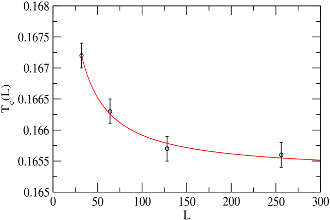
Figure 24: Estimated peak values $T_{c}(L)$ versus $L$ along with an extrapolation $T_{c}+c/L$ (solid line).

5 Summary

Machine learning methods provide the opportunity to study phase transitions without a priori specification of an order parameter or other thermodynamic function. In this work two different methods, principal component analysis and support vector machines, have been applied to the Blume-Capel and Biquadratic Spin-1 Ising models. These classical spin models can exhibit different transition behaviour for different values of their model parameters. PCA and SVM can expose both the presence and nature of these transitions.

PCA is an unsupervised method which is useful when the data have a few dominant features. As discussed in [2], and reproduced here, a plot of the leading principal components provides useful qualitative information about the model’s phase behaviour using as input raw Monte Carlo simulation data (see Figs. 3,13 ). PCA typically identifies the magnetization as the dominant feature without input of any domain knowledge.

SVM is a supervised method trained for the models studied here as a binary classifier for Monte Carlo data generated at two different points in temperature or in the model parameter space. The trained decision function can be used to determine the presence of a phase transition separating training points. We showed examples from the Blume-Capel and Biquadratic Spin-1 Ising models how the standard deviation of the decision function interpolated between the training points provides a proxy for the susceptibility. As suggested in [7], SVM can provide quantitative information without a priori knowledge of an order parameter. As an example of a quantitative analysis the critical temperature for the BSI model at $K$ = 1, $J$ = 0.1 was determined to be 0.1655(5), close to the value given in [2].

References

- [1] Lei Wang, Phys. Rev. B 94, 195105 (2016).
- [2] W. Hu, R. R. P. Singh and R. T. Scalettar, Phys. Rev. B 95, 062122 (2017).
- [3] S. J. Wetzel, Phys. Rev. E 96, 022140 (2017).
- [4] S. J. Wetzel and M. Scherzer, Phys. Rev. B 96, 205146 (2017).
- [5] J. Carrasquilla and R. G. Melko, Nature Phys. 13, 431 (2017).
- [6] P. Ponte and R. G. Melko, Phys. Rev. B 96, 205146 (2017).
- [7] C. Giannetti, B. Lucini and D. Vadacchino, arXiv:1812.06726.
- [8] C. Alexandrou, A. Athenodorou, C. Chrysostomou and S. Paul, arXiv:1903.03506.
- [9] J. Shlens, A Tutorial on Principal Component Analysis, arXiv:1404.1100.
- [10] F. Pedregosa et al., J. Machine Learning Res. 12, 2825 (2011).
- [11] https://scikit-learn.org/stable/modules/svm.html
- [12] L. Onsager, Phys. Rev. 65, 117 (1944).
- [13] C. N. Yang, Phys. Rev. 85, 808 (1952).
- [14] M. Blume Phys. Rev. 141, 517 (1966).
- [15] H. W. Capel Physica 32, 966 (1966).
- [16] J. C. Xavier, F. C. Alcaraz, D. P. Lara and J. A. Plascak, Phys. Rev. B 57, 11575 (1998).
- [17] S. M. Pittman, G. G. Batrouni and R. T. Scalettar, Phys. Rev. B 78, 214208 (2008).
- [18] W. Kwak, J .Jeong, J. Lee and D. H. Kim, Phys. Rev. E 78, 022134 (2015).