Gas of baby universes in JT gravity and matrix models

Abstract

It has been shown recently by Saad, Shenker and Stanford that the genus expansion of a certain matrix integral generates partition functions of Jackiw-Teitelboim (JT) quantum gravity on Riemann surfaces of arbitrary genus with any fixed number of boundaries. We use an extension of this integral for studying gas of baby universes or wormholes in JT gravity. To investigate the gas nonperturbatively we explore the generating functional of baby universes in the matrix model. The simple particular case when the matrix integral includes the exponential potential is discussed in some detail. We argue that there is a phase transition in the gas of baby universes.

1 Introduction

It has been shown by Saad, Shenker and Stanford SSS that the genus expansion of a certain matrix integral generates the partition functions of Jackiw-Teitelboim (JT), Jackiw:1984je ; Teitelboim:1983ux , quantum gravity on Riemann surfaces of arbitrary genus with an arbitrary fixed number of boundaries. It is shown in SSS that an important part of JT quantum gravity is reduced to computation of the Weil-Petersson volumes of the moduli space of hyperbolic Riemann surfaces with various genus and number of boundaries for which Mirzakhani Mir established recursion relations. Eynard and Orantin eynard2007invariants ; EO proved that Mirzakhani’s relations are a special case of random matrix recursion relations with the spectral curve $y=\sin(2\pi z)/4\pi$. This is a natural extension of results on topological gravity Witten-2gr ; MK ; ManinZograf ; DW . Relation of random matrices and gravity, including black hole description, has a long history, see Cotler:2016fpe ; Saad:2018bqo and refs therein.

The results of SSS provide a nonperturbative approach to JT quantum gravity on Riemann surfaces of various genus and perturbative description of boundaries. We use an extension of this result for nonperturbative studying of gas of baby universes in JT gravity. To investigate the boundaries nonperturbatively we explore the generating functional of boundaries in the matrix model and in JT gravity. One interprets the generating functional as the partition function of gas of baby universes in grand canonical ensemble in JT multiverse with the source function describing the distribution of boundaries being treated as the chemical potential. The interaction is presented by splitting and joining of baby universes.

Let $Z^{grav}_{g,n}(\beta_{1},...,\beta_{n})$ be the JT gravity path integral for Riemann surface of genus $g\geq 2$ with $n$ boundaries with lengths $\beta_{1},...,\beta_{n}$. Consider a generating function for these functions

$${\mathcal{Z}}_{n}^{grav}(\beta_{1},...,\beta_{n};\gamma)\simeq\sum_{g=0}^{\infty}\gamma^{2g+n-2}{\mathcal{Z}}_{g,n}^{grav}(\beta_{1},...,\beta_{n})$$ (1)

where $\gamma$ is a constant which in notations of SSS is $\gamma=e^{-S_{0}}$.

The following remarkable relation between correlation functions in matrix model and JT gravity holds SSS :

$${\mathcal{Z}}_{n}^{matrix,d.s.}(\beta_{1},...,\beta_{n};\gamma)\simeq Z^{grav}_{n}(\beta_{1},...,\beta_{n};\gamma)$$ (2)

Here ${\mathcal{Z}}_{n}^{matrix,d.s.}(\beta_{1},...,\beta_{n};\gamma)$ is the double scaling (d.s.) limit of the correlation function in a matrix model with the spectral curve mentioned above. This form of the curve was obtained in SSS by computing the JT path integral for the disc.

In this note we consider the generating functional for the gravitational correlation functions $Z^{grav}_{n}(\beta_{1},...,\beta_{n};\gamma)$

$${\cal Z}^{grav}(J;\gamma)=\sum_{n=0}^{\infty}\frac{1}{n!}\int_{0}^{\infty}d\beta_{1}...\int_{0}^{\infty}d\beta_{n}Z^{grav}_{n}(\beta_{1},...,\beta_{n};\gamma)J(\beta_{1})...J(\beta_{n})\\$$ (3)

where $J(\beta)$ is a source function. An appropriate generating functional in matrix theory has the form

$$\mathfrak{Z}^{matrix}(J)=<\mathrm{e}^{N\int\!Z(\beta)J(\beta)d\beta}>$$ (4)

$$=\sum_{n=0}^{\infty}\frac{N^{n}}{n!}\int\!\!d\beta_{1}...\int\!\!d\beta_{n}{\mathcal{Z}}_{n}^{matrix}(\beta_{1},...\beta_{n})J(\beta_{1})...J(\beta_{n})$$

(5)

Here $Z(\beta)={\rm Tr}e^{-\beta M}$ where $M$ is a random $N\times N$ Hermitian matrix. This amounts to shifting the potential in the matrix model $V(x)\to V(x)-\widetilde{J}(x)$ where $\widetilde{J}(x)$ is the Laplace transform of $J(\beta)$, see Sect.2.

We define the generating functional for connected correlation functions

$$\mathfrak{G}^{matrix}(J)=-\frac{1}{N^{2}}\log\mathfrak{Z}^{matrix}(J)$$ (6)

take the double scaling limit introducing the parameter $\gamma$ and obtain the relation between JT gravity and the matrix model in terms of the generating functionals:

$$d.s.\lim\mathfrak{G}^{matrix}(J)\simeq\mathfrak{Z}^{\text{grav}}(J;\gamma)$$ (7)

The ”$\simeq$” symbol indicates the equality in the sense of formal series.

The paper is organized as follows. In Sect.2 the generating functional in matrix theory $\mathfrak{Z}^{matrix}(J)$ is discussed. Here $J$ is the source function. In Sect.3 the generating functional of boundaries in JT gravity $\mathfrak{Z}^{grav}(J)$ is considered. In Sect.4 we investigate the double scaling limit in matrix models with a particular choice of the source $J(\beta)$ which leads to the change of the potential $V(x)\to V(x)-Je^{\omega x}$. In Sect.5 the matrix model with the exponential potential is investigated. In Sect.6 the matrix model with the spectral curve $y=\sin(2\pi z)/4\pi$ and the source is discussed and phase transition is observed. In Sect.7 the discussion of obtained results is presented.

2 Generating functional in matrix models

Generating functional. We consider ensemble of $N\times N$ Hermitian matrices Wigner ; Dyson ; BIPZ ; mehta with potential $V(M)$. Let

$$Z(\beta)={\rm Tr}e^{-\beta M}=\sum_{i=1}^{N}\exp(-\beta\lambda_{i}),\,\,\,\beta>0.$$ (8)

where $\lambda_{i}$ are eigenvalues of the matrix $M$. The $n$-point correlation function of $Z(\beta)$ in the matrix model is given by

$$\,\,\,\,\,\,\,\,\,\,\,\,\,\,{\mathcal{Z}}^{matrix}_{n}(\beta_{1},...,\beta_{n})\equiv<Z(\beta_{1})...Z(\beta_{n})>$$ (9)

$$= \int Z(\beta_{1})...Z(\beta_{n})\exp(-N{\rm Tr}V(M))dM/\int\exp(-N{\rm Tr}V(M))dM$$

Its generating functional can be presented as

$$\mathfrak{Z}^{matrix}(J)=<\mathrm{e}^{N\int\!Z(\beta)J(\beta)d\beta}>=\sum_{n=0}^{\infty}\frac{N^{n}}{n!}\int\!\!d\beta_{1}...\int\!\!d\beta_{n}{\mathcal{Z}}_{n}^{matrix}(\beta_{1},...\beta_{n})J(\beta_{1})...J(\beta_{n})$$

(10)

or

$$\mathfrak{Z}^{matrix}(J)=\int\exp\{N\sum_{j=1}^{N}\widetilde{J}(\lambda_{j})\}\,d\mu_{N}(\lambda_{1},...\lambda_{N})$$ (11)

where

$$d\mu_{N}(\lambda_{1},...\lambda_{N}) = \frac{1}{Z_{N}}\prod_{j>k}(\lambda_{j}-\lambda_{k})^{2}\prod_{j=1}^{N}e^{-NV(\lambda_{j})},$$ (12)

$$\widetilde{J}(\lambda) = \int d\beta J(\beta)\mathrm{e}^{-\beta\lambda}d\beta$$ (13)

This amounts to shift the potential $V(x)\to V(x)-\widetilde{J}(x)$.

One expands $\mathfrak{G}(J)=\log\mathfrak{Z}^{matrix}(J)$ to get the connected correlation functions

$$\mathfrak{G}^{matrix}(J)=\sum_{n=0}^{\infty}\frac{1}{n!}\int\!\!d\beta_{1}...\int\!\!d\beta_{n}{\mathcal{Z}}_{n,conn}^{matrix}(\beta_{1},...\beta_{n})J(\beta_{1})...J(\beta_{n})$$

(14)

Particular case. We consider a special case

$$J(\beta)=-J\delta(\beta+\omega)$$ (15)

In this case the consideration of $\mathfrak{Z}^{matrix}(J)$ is equivalent to dealing with the matrix model with a deformed potential

$$U(x)=V(x)+J\mathrm{e}^{\omega x}$$ (16)

In this case the singular integral equation defining the eigenvalues distribution has the form

$$U^{\prime}(\lambda)=2\fint_{{\mathcal{S}}}d\mu\frac{\rho(\mu)}{\lambda-\mu},$$ (17)

and the spectral density is

$$\rho(\mu)=\lim_{N\to\infty}\frac{1}{N}<\sum_{i=1}^{N}\delta(\mu-\lambda_{i})\exp\{-NJ\sum_{j=1}^{N}e^{\omega\lambda_{j}}\}>$$ (18)

Double scaling limit. All the correlation functions ${\mathcal{Z}}^{matrix}_{n}(\beta_{1},...,\beta_{n})$ in principle could be derived if the potential $V(x)$ or the spectral density/spectral curve $\rho(\mu)$ is known. To get a connection of the matrix model with JT gravity one has to go to the double scaling limit, see SSS . Consider a matrix model with a non-normalized spectral density

$$\rho^{\text{nnorm}}(E)=\frac{e^{S_{0}}}{(2\pi)^{2}}\sinh\left(2\pi\sqrt{\frac{a^{2}-E^{2}}{2a}}\right),\hskip 20.0pt-a<E<a.$$ (19)

where $S_{0}$ is a constant. Now, shifting $E\to E-a$ and sending $a\to\infty$ we get the spectral density of the double-scaled matrix model

$$\rho_{d.s.}^{\text{nnorm}}(E)=\frac{e^{S_{0}}}{(2\pi)^{2}}\sinh(2\pi\sqrt{E}),\,\,\,\,\,\,\,\,\,\,E>0.$$ (20)

and the correlation functions in the double scaled limit

$$d.s.\lim{\mathcal{Z}}_{n,conn}^{matrix}(\beta_{1},...\beta_{n})={\mathcal{Z}}_{n}^{matrix,d.s.}(\beta_{1},...,\beta_{n})$$ (21)

The limiting correlation functions ${\mathcal{Z}}_{n}^{matrix,d.s.}(\beta_{1},...,\beta_{n})$ have an expansion of the form

$${\mathcal{Z}}_{n}^{matrix,d.s.}(\beta_{1},...,\beta_{n})\simeq\sum_{g=0}^{\infty}(e^{-S_{0}})^{2g+n-2}{\mathcal{Z}}_{g,n}^{matrix,d.s.}(\beta_{1},...,\beta_{n})$$ (22)

The double scaling limit of the generating functional is

$$d.s.\lim\log\mathfrak{Z}^{matrix}(J)=\sum_{n=0}^{\infty}\frac{1}{n!}\int\!\!d\beta_{1}...\int\!\!d\beta_{n}{\mathcal{Z}}_{n}^{matrix,\,d.s.}(\beta_{1},...\beta_{n})J(\beta_{1})...J(\beta_{n})$$

(23)

The correlation functions ${\mathcal{Z}}_{g,n}^{matrix,\,d.s.}(\beta_{1},...,\beta_{n})$ and the constant $S_{0}$ will be used in the next section to describe the connection of the matrix model with JT gravity. The double scaling limit will be discussed also in Sect.4.

Resolvents. Similarly one has generating functional for correlation functions of resolvents

$$\mathfrak{R}^{(matrix)}(f)=<\mathrm{e}^{N\int R(z)f(z)dz}>$$ (24)

where $f(z)$ is a test function and

$$R(z)={\rm Tr}(z-M)^{-1}.$$ (25)

Expanding $\log\mathfrak{R}^{(matrix)}(f)$ in the series on $f$ one gets connected correlation functions $<R(z_{1})...R(z_{n})>_{c}$. We perform the double scaling limit

$$d.s.\lim<R(z_{1})...R(z_{n})>_{c}=<R(z_{1})...R(z_{n})>_{c}^{d.s.}$$ (26)

which admits an expansion

$$<R(z_{1})...R(z_{n})>_{c}^{d.s.}\simeq\sum_{g=0}^{\infty}\frac{1}{(e^{S_{0}})^{2g+n-2}}R_{g,n}(z_{1},...,z_{n})$$ (27)

One defines the correlation functions

$$W_{g,n}^{matrix}(z_{1},...,z_{n})=(-1)^{n}2^{n}\,z_{1}...z_{n}\,R_{g,n}(-z_{1}^{2},...,-z_{n}^{2})$$ (28)

which satisfy the loop equations migdal ; AJM ; eynard and will be used in the next section, and the generating functional

$${\cal W}_{g}(f)=\sum_{n=0}^{\infty}\frac{1}{n!}\int dz_{1}...\int dz_{n}W_{g,n}^{matrix}(z_{1},...,z_{n})f(z_{1})...f(z_{n}).$$ (29)

3 Generating functional in JT gravity

The Euclidean action of JT gravity Jackiw:1984je ; Teitelboim:1983ux ; Almheiri:2014cka has the form

$$I_{JT}=-\frac{S_{0}}{2\pi}\left[\frac{1}{2}\int_{\mathcal{M}}\sqrt{g}R+\int_{\partial\mathcal{M}}\sqrt{h}K\right]-\left[\frac{1}{2}\int_{\mathcal{M}}\sqrt{g}\phi(R+2)+\int_{\partial\mathcal{M}}\sqrt{h}\phi(K-1)\right].$$ (30)

Here $g_{\mu\nu}$ is a metric on a two dimensional manifold $\mathcal{M}$, $\phi$ is a scalar field (dilaton) and the constant $S_{0}$ was mentioned in the previous section. The path integral for Riemann surface of genus $g\geq 2$ with $n$ boundaries with lengths $\beta_{1},...,\beta_{n}$ reads

$$Z^{grav}_{g,n}(\beta_{1},...,\beta_{n})=e^{-S_{0}\chi}\int\frac{\mathcal{D}g_{\mu\nu}\mathcal{D}\phi}{\text{Vol}(\text{diff})}\,e^{-{\widehat{I}}_{JT}[g_{\mu\nu},\phi]}$$ (31)

where $\chi$ is the Euler characteristic $\chi=2-2g-n$ and ${\widehat{I}}_{JT}$ is the JT action with the first $S_{0}$ term left out.

The following relation between the matrix model and JT gravity holds SSS :

$${\mathcal{Z}}_{g,n}^{matrix,d.s.}(\beta_{1},...,\beta_{n})=Z^{grav}_{g,n}(\beta_{1},...,\beta_{n})$$ (32)

or

$${\mathcal{Z}}_{n}^{matrix,d.s.}(\beta_{1},...,\beta_{n})\simeq Z^{grav}_{n}(\beta_{1},...,\beta_{n})$$ (33)

where

$${\mathcal{Z}}_{n}^{grav}(\beta_{1},...,\beta_{n})\simeq\sum_{g=0}^{\infty}(e^{-S_{0}})^{2g+n-2}{\mathcal{Z}}_{g,n}^{grav}(\beta_{1},...,\beta_{n})$$ (34)

It was found in SSS that the partition function has the form $(g\geq 2)$

$$Z^{grav}_{g,n}(\beta_{1},...,\beta_{n})=\int_{0}^{\infty}b_{1}db...\int_{0}^{\infty}b_{n}db_{n}V_{g,n}(b_{1},...,b_{n})Z_{\text{Sch}}^{\text{trumpet}}(\beta_{1},b_{1})...Z_{\text{Sch}}^{\text{trumpet}}(\beta_{n},b_{n})$$ (35)

where $V_{g,n}(b_{1},...,b_{n})$ is the Weil-Petersson volume of the moduli space of a genus $g$ Riemann surface with $n$ geodesic boundaries of lengths $b_{1},...,b_{n}$ and

$$Z_{\text{Sch}}^{\text{trumpet}}(\beta,b)=\frac{1}{2\pi^{1/2}\beta^{1/2}}e^{-\frac{b^{2}}{4\beta}}.$$ (36)

From this we get

$${\cal Z}^{grav}_{g}(J)=\sum_{n=0}^{\infty}\frac{1}{n!}(e^{-S_{0}})^{2g+n-2}\int_{0}^{\infty}d\beta_{1}...\int_{0}^{\infty}d\beta_{n}Z^{grav}_{g,n}(\beta_{1},...,\beta_{n})J(\beta_{1})...J(\beta_{n})$$ (37)

$$=\sum_{n=0}^{\infty}\frac{1}{n!}(e^{-S_{0}})^{2g+n-2}\int_{0}^{\infty}b_{1}db...\int_{0}^{\infty}b_{n}db_{n}V_{g,n}(b_{1},...,b_{n}){\widehat{J}}(b_{1})...{\widehat{J}}(b_{n}),$$ (38)

where

$${\widehat{J}}(b)=\int_{0}^{\infty}d\beta\frac{1}{2\pi^{1/2}\beta^{1/2}}e^{-\frac{b^{2}}{4\beta}}J(\beta)$$ (39)

and the generating functional

$$\mathfrak{Z}^{grav}(J)\simeq\sum_{g=0}^{\infty}{\cal Z}^{grav}_{g}(J)$$ (40)

Finally, one obtains the relation

$$d.s.\lim\log\mathfrak{Z}^{matrix}(J)\simeq\mathfrak{Z}^{\text{grav}}(J)$$ (41)

Similarly, the correlation functions $W_{g,n}^{matrix}$ are related with volumes of the moduli spaces as

$$W_{g,n}^{matrix}(z_{1},...,z_{n})=\int_{0}^{\infty}b_{1}db_{1}e^{-b_{1}z_{1}}...\int_{0}^{\infty}b_{n}db_{n}e^{-b_{n}z_{n}}V_{g,n}(b_{1},...,b_{n}).$$ (42)

The generating functional is

$${\cal Z}_{R,g}(f)=\sum_{n=0}^{\infty}\frac{1}{n!}\int dz_{1}...\int dz_{n}W_{g,n}^{matrix}(z_{1},...,z_{n})f(z_{1})...f(z_{n})$$

$$= \sum_{n=0}^{\infty}\frac{1}{n!}\int_{0}^{\infty}b_{1}db_{1}...\int_{0}^{\infty}b_{n}db_{n}V_{g,n}(b_{1},...,b_{n})\widetilde{f}(b_{1})...\widetilde{f}(b_{n})$$

where

$$\widetilde{f}(b)=\int dze^{-bz}f(z).$$ (43)

Baby universes. In cosmology HL ; LRT ; GS ; Coleman ; IV ; 1807.00824 , one usually deals with baby universes that branch off from, or join onto, the parent(s) Universe(s). In matrix theories one parent is a connected Riemann surface with arbitrary number of handles and at least one boundary. We assume that the lengths of boundaries of baby universities are small as compare with the boundary length of the parent, see Fig.1. Baby universes are attached to the parent by necks that have restricted lengths of geodesics at which the neck is attached to the parent, We assume that the lengths of the boundaries of baby universes are small compared to the length of the boundary of the parent, see Fig. 1. Baby universes are attached to the parent with the help of thin necks. Thickness of the neck is defined as the geodesic length of the loop located at the thinness point of the neck, and this length is assumed to be essentially smaller than the length of theboundary of the parent, see Fig.1.b and Fig.1.c. There are also restrictions on the area of the surface of baby universes, see Mathur ; Renata for more precise definitions. Cosmological baby universes in the parent-baby universe approximation interact only via coupling to the parent universes, that themselves interact via wormholes. In matrix models the baby universes always interact via their parents too and parents interact via wormholes, Fig.2. One can expect that at large number of baby universes interaction between different parts of the system increases and this leads to phase transition (an analog of the the nucleation of a baby universe in GS ). We interpret the matrix partition function $\mathfrak{Z}$, defined by equation (23) as a partition function of the gas of baby universes.

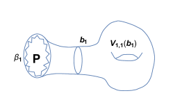
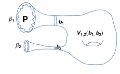
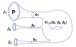
+ … (a)                         (b)                         (c)

Figure 1: Gas of baby universes. Here $|\beta_{1}|>>|\beta_{i}|$ for $i\geq 2$ and $b_{i}\leq b_{c}$ for $i\geq 2$

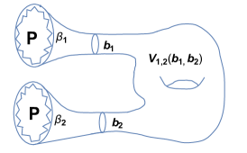
Figure 2: Two parents connected by the wormhole

4 Double scaling limit

4.1 Double scaling limit for the GUE

There are various notions of the double scaling limit in matrix theory doublescaling ; DS ; GM ; DFGZ ; MM ; Ey5Lectures ; bz1 ; BB ; BI ; Pastur ; Widom ; KM ; DKMVZ . A special double scaling limit was considered in SSS at the level of spectral density. Here we discuss it at the level of the potentials. We will see that the linear term in the potential plays a special role.

Let us start with the Wigner distribution for the Gaussian Unitary Ensemble (GUE) Wigner ; Dyson ; BIPZ ; mehta . The ordinary Wigner distribution $2\sqrt{a^{2}-\lambda^{2}}/\pi a^{2}$ is supported on the interval $[-a,a]$ and is obtained from a matrix model with the potential $V(x)=m^{2}x^{2}/2$, where $m^{2}={\color[rgb]{1,0,0}4}/a^{2}$. We want to make a shift and get a distribution on the interval $[0,\Lambda]$, $\Lambda>0.$ To this end we consider the gaussian model with an external source

$$V(x)=m^{2}\left(\frac{1}{2}\,x^{2}+jx\right)$$ (44)

and we make parameters $m$ and $j$ depending on $\Lambda$ to put the measure support on $[0,\Lambda]$. The singular integral equation defining the density takes the form

$$m^{2}(\lambda+j)=2\fint_{\,{}_{[0,\Lambda]}}d\lambda^{\prime}\frac{\rho_{W}(\lambda^{\prime})}{\lambda-\lambda^{\prime}}$$ (45)

Here $\fint$ means the Cauchy principal value of the integral. The solution of (45) is given by the shifted Wigner distribution

$$\rho_{W}(\lambda) = \frac{8}{\pi\Lambda^{2}}S_{\Lambda}(\lambda),\,\,\,\,\,\,S_{\Lambda}(\lambda)=\sqrt{\lambda(\Lambda-\lambda)}$$ (46)

Note that the constant $j$ from the linear term in the potential does not enter into the expression for the spectral density. This is valid for any potential. The constant appears only throughout the normalization and consistency conditions that in this case read

$$m^{2}\Lambda^{2}=16,\,\,\,\,\,\,\,\,\Lambda=-2j$$ (47)

We get that the eigenvalue density (46) is supported by the potential

$$V_{\Lambda}(x)=\frac{4}{\Lambda^{2}}(\frac{1}{2}x^{2}-\Lambda x)$$ (48)

in the sense that

$$\rho_{W}(\lambda) = \lim_{N\to\infty}\,\rho^{V_{\Lambda}}_{N}(\lambda)$$ (49)

where

$$\rho^{V_{\Lambda}}_{N}(x)=\frac{1}{N}<{\rm Tr}\delta(x-M)>_{\!{}_{V_{\Lambda}}}$$ (50)

$<f>_{\!{}_{V}}$ in (50) means averaging with potential $<f>_{\!{}_{V}}=\int\!\!fe^{-N{\rm Tr}V}dM/\int\!\!e^{-N{\rm Tr}V}dM.$

Now we take the limit $\Lambda\to\infty$ and write

$$\lim_{\Lambda\to\infty}\,\Lambda^{\eta}\,\rho_{W}(\lambda)=\frac{8}{\pi}\sqrt{\lambda},\,\,\,\,\lambda\in[0,\Lambda],$$ (51)

where $\eta=3/2$. So, we get an expected result in two steps. First we send $N\to\infty$ and then $\Lambda\to\infty$.

One can use also another procedure. Set $\Lambda=t\,N$ and in this case one has

$$\lim_{N\to\infty}\,(N)^{3/2}\,\rho^{V_{tN}}_{N}(\lambda)=\frac{8}{t^{3/2}\pi}\sqrt{\lambda}\$$ (52)

where

$$V_{tN}(x)=\frac{2}{t^{2}N^{2}}x^{2}-\frac{4}{tN}x$$ (53)

4.2 Double scaling limit for the cubic interaction

Let us consider the matrix model with the potential

$$V(x)=m^{2}(\frac{1}{2}x^{2}+jx+\frac{1}{3}gx^{3})$$ (54)

and we will make parameters $m,j,g$ depending on $\Lambda$ to put the support of the spectral density on $[0,\Lambda]$. Again first we take the limit $N\to\infty$ and then the limit $\Lambda\to\infty$. In the large $N$ limit one gets the singular integral equation that defines the spectral density

$$m^{2}(\lambda+j+g\lambda^{2})=2\fint_{[0,\Lambda]}d\lambda^{\prime}\frac{\rho(\lambda^{\prime})}{\lambda-\lambda^{\prime}}$$ (55)

We write solution in the form

$$\rho(\lambda) = \frac{m^{2}\,S_{\Lambda}(\lambda)}{2\pi^{2}}\int_{0}^{\Lambda}\,\frac{1+g(\lambda+\lambda^{\prime})}{S_{\Lambda}(\lambda^{\prime})}\,d\lambda^{\prime},$$ (56)

$S_{\Lambda}(\lambda)$ is given by (46), and we get

$$\rho(\lambda) = \frac{m^{2}\,S_{\Lambda}(\lambda)}{2\pi^{2}}\Big{(}1+g\lambda+g\frac{\Lambda}{2}\Big{)}.$$ (57)

The normalization condition is achieved by a suitable choice of $m^{2}$,

$$m^{2}\Lambda^{2}\Big{(}1+g\Lambda\Big{)} = 16$$ (58)

and the consistency condition by the suitable choice of j

$$4\Lambda+g3\Lambda^{2}+8j = 0.$$ (59)

The solution of these equations is evidently

$$m^{2}=16/\Lambda^{2}\Big{(}1+g\Lambda\Big{)},\,\,j=-(4\Lambda+g3\Lambda^{2})/8$$ (60)

which should be substituted into the potential. Now we take the large $\Lambda$ limit and get

$$\lim_{\Lambda\to\infty}\Lambda^{3/2}\rho(\lambda)=\frac{4}{\pi^{2}}\sqrt{\lambda}.$$ (61)

More reach picture appears for the quartic interaction with negative mass square. In this case for suitable choice of parameters there is a double cut solution AIM ; CCM , universality of the double scaling limit in this case has been proved in BI , see also CM for more general multi-cut solutions.

5 Deformation by an exponential potential

5.1 Exponential potential

Here we consider a deformation of the Wigner distribution by the insertion of the exponential potential

$$U(x)=V_{0}(x)+V_{1}(x)=\frac{m^{2}x^{2}}{2}+Je^{\omega x}$$ (62)

There are 4 different choices of signs of $J$ and $\omega$, see Fig.3. We see that only $J<0$ may produce some non trivial effects due to an appearance of potential instability, Fig.3.c and Fig.3.d. The choice of sign of $\omega$ is irrelevant.

            

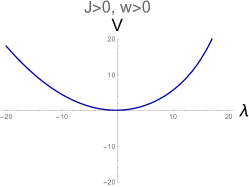
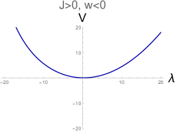
(a)                                                  (b)

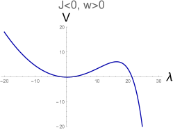
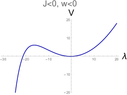
(c)                                                  (d)

Figure 3: Four different choices of perturbations of the gaussian ensemble by the exponential potential $V_{1}=Je^{\omega x}$.

Fig.4 shows an appearance of a phase transition under a perturbation of the gaussian model by the exponential potential $V_{\exp}=Je^{\omega\lambda}$ taken with positive $J$ and $w=0.25$. We see that the minimum of the potential disappears when $m$ decreases, Fig.4.a, or $|J|$ increases for negative $J$, Fig.4.b.

          

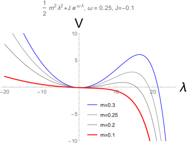
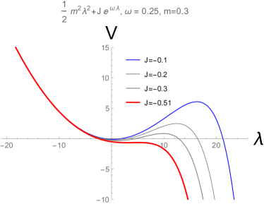
(a)                                                  (b)

Figure 4: The appearance of phase transition under perturbation of the gaussian model by the exponential potential $\Delta V=Je^{\omega\lambda}$ taken with positive $J$ and $w=0.25$.

The shift of $\lambda\to\lambda+\delta\lambda$ in the potential (62) produces the linear term in the potential and multiplies the current $J$ on the constant $J\to J\mathrm{e}^{\delta\lambda}$. We parametrize our potential as

$$V(x)=m^{2}\Big{(}\frac{1}{2}x^{2}+Cx+J\,\mathrm{e}^{\omega x}\Big{)}$$ (63)

and fix the parameters in (63) in an agreement with the measure localization on the segment $[0,\Lambda]$. To this purpose we first find the non-normalized measure as a sum of non-normalized ones corresponding to the shifted Wigner and exponential potential distributions $\rho_{W}(\lambda,\Lambda)$ and $\rho_{e^{w\lambda}}(\lambda,\Lambda,\omega)$.

The forms of non-normalized measures $\rho_{e^{w\lambda}}(\lambda)$ for positive and negative $w$ presented are presented in Fig.5.

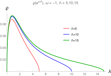
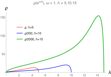
(a)                                                  (b)

Figure 5: Non–normalized density plot for the exponential potential with negative $\omega=-1$ (a) and positive $\omega=1$ (b) and different regularization parameter $\Lambda$.

We can compare the contribution to the non-normalized density from the Wigner semi-circle for mass equal to 1 and the exponential potential taken with arbitrary current $J$. We see that this sum always defines the positive density for $J>0$ and becomes negative for $J<J_{cr}(\Lambda,\omega)<0$. Then for $J>J_{cr}(\Lambda,\omega)$ we find relation between $m^{2}$ and $\Lambda,\omega$ and $J$ from normalization condition.

In Fig.6 the appearance of the phase transition at negative $J$ is presented. In Fig. 7.a relations between $m^{2}$ and $J$ for fixed $\Lambda$ and $\omega$ are shown for different values of $\Lambda$ and in Fig.7.b.

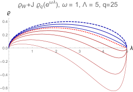
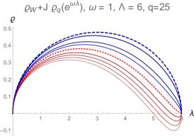
(a)                                                  (b)

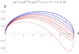
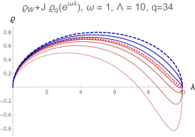
(c)                                                  (d)

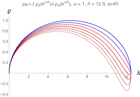
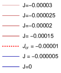
(e)                                                  (f)

Figure 6: The plot of non–normalized density for the quadratic potential deformed by the exponential potential for different values of the regularization parameter $\Lambda$ and $\omega=1$.

We can present the eigenvalues distribution corresponding to the potential (63) as a sum

$$\rho_{nn}(\lambda)=\rho_{W}(\lambda,\Lambda)+J\rho_{e^{w\lambda}}(\lambda,\Lambda,\omega)$$ (64)

where

$$\rho_{W}(\lambda) = \frac{1}{2\pi^{2}}\sqrt{\lambda(\Lambda-\lambda)}\int^{\Lambda}_{0}\,\frac{d\mu}{\sqrt{(b-\mu)(\mu-a)}}$$ (65)

$$\rho_{e^{w\lambda}}(\lambda) = \frac{\omega}{2\pi^{2}}\sqrt{\lambda(\Lambda-\lambda)}\int^{\Lambda}_{0}\,\frac{(e^{\omega\lambda}-e^{\omega\mu})d\mu}{(\lambda-\mu)\sqrt{(b-\mu)(\mu-a)}}$$ (66)

and fix constant $C$ and $m^{2}$ from the consistency condition and normalization, respectively,

$$0 = \int_{0}^{\Lambda}\frac{\lambda+C+J\,\omega e^{\omega\lambda}}{S_{\Lambda}}\,d\lambda$$ (67)

$$\frac{1}{m^{2}} = \int_{0}^{\Lambda}\Big{(}\rho_{W}(\lambda,\Lambda)+J\rho_{e^{w\lambda}}(\lambda,\Lambda,\omega)\Big{)}\,d\lambda$$ (68)

The forms of non-normalized measures $\rho_{e^{w\lambda}}(\lambda)$ for positive and negative $w$ presented are presented in Fig.5. We see that these two segment distributions are nonsymmetric under the centre of the segment. The distribution of eigenvalues for the case of negative $\omega$ is pressed to the left boundary of the segment, and the for the case of positive $\omega$ it is pressed to the right one. Applying this deformation with a positive $J$ to the GUE we ”activate” the left or right part of of eigenvalues. Applying the same with negative $J$ we can destroy the constructed solution. We compare the contribution to the non-normalized density from the Wigner semi-circle for mass equal to 1 and the exponential potential taken with arbitrary current $J$. We see the this sum always define the positive density for $J>0$ and becomes negative for $J<J_{cr}(\Lambda,\omega)<0$. Then $J>J_{cr}(\Lambda,\omega)$ we find relation between $m^{2}$ and $\Lambda,\omega$, and $J$ from normalization condition.

In Fig.6 is presented the appearance of the phase transition at negative $J$ for different $\Lambda$. We see that for chosen parameters, $m^{2}=1,\omega=1$ the critical $J_{cr}$ decreases with increasing $\Lambda$. To find the real mass that supports the normalized solution,

$$\rho(\lambda)=n(\lambda)\rho_{nn}(\lambda)$$ (69)

we find $n(\lambda)$ from the normalization condition, so

$$n(\Lambda)^{-1}=\int_{0}^{\Lambda}\rho_{nn}(\lambda)d\lambda$$ (70)

and assume that the mass is given my

$$m^{2}=n(\Lambda)$$ (71)

In Fig.7.a the dependence of $m^{2}$ on $J$ for fixed $\Lambda$ and $\omega$ is shown for different values of $\Lambda$. Here $J>J_{cr}(\Lambda)$. We see that mass (in our parametrization of the potential of the model) decreases with increasing $J$. The slow of the mass is more fast for larger $\Lambda$.

                     

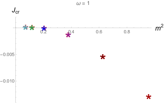
(a)                                                  (b)

Figure 7: (a) Relations between $m^{2}$ and $J$ for fixed $\Lambda$ and $\omega$. (b) The mass square at $J_{cr}$ for $\omega=1$. The legend is the same as at (a).

In Fig.7.b the dependence of the critical current $J_{cr}$ on mass is shown. We see that $J_{cr}$ goes to zero when $m^{2}$ goes to zero, that corresponds to increasing $\Lambda$.

 

5.2 Fine tuning

It is obvious that fixing from the beginning the location of the eigenvalue one immediately gives restrictions on parameters of the potential of the matrix model. If we want to shift the location of the eigenvalues, ${\mathcal{S}}_{[a,b]}\to{\mathcal{S}}_{[0,b-a]}$ we have to make a shift in the potential, $V(x)\to V(x+a)$. For the quadratic potential this shift produces the linear term $\Delta V(x)=jx$ and $j$ can be determined from the location of the left point of the cut. For higher polynomial interaction the shift produces the linear term in the LHS of singular equation, as well as change of coupling constants. The shift in the exponential potential produces just a multiplication on positive constant.

We have also seen that if we want to deform a given distribution by a new potential, that has the same locations of eigenvalues, we can just take the sum of the given two distributions and multiply all coupling constants of two initial model on the same parameter to fix the normalization condition for the distributions that is the some of given two distributions. As to the consistency condition it follows from consistency conditions of individual distributions. More precisely, if we know that

$$V^{\prime}_{1}(\lambda) = 2\fint_{\mathcal{S}}\frac{\rho_{V_{1}}(\lambda^{\prime})}{\lambda-\lambda^{\prime}}d\lambda^{\prime}\,,\,\,\,\,\,\,\,\int_{\mathcal{S}}\rho_{V_{1}}(\lambda)d\lambda=1$$ (72)

$$V^{\prime}_{2}(\lambda) = 2\fint_{\mathcal{S}}\frac{\rho_{V_{2}}(\lambda^{\prime})}{\lambda-\lambda^{\prime}}d\lambda^{\prime}\,,\,\,\,\,\,\,\,\int_{\mathcal{S}}\rho_{V_{2}}(\lambda)d\lambda=1,$$ (73)

Note that in both integrals the segment is the same. Taking

$$\rho_{T}=\frac{1}{2}(\rho_{V_{1}}+\rho_{V_{2}})$$ (74)

we can claim that $\rho_{T}$ solves equations

$$V^{\prime}_{T}(\lambda)\equiv\frac{1}{2}(V^{\prime}_{1}(\lambda)+V^{\prime}_{2}(\lambda)) = 2\fint_{\mathcal{S}}\frac{\rho_{T}(\lambda^{\prime})}{\lambda-\lambda^{\prime}}d\lambda^{\prime}\,,\,\,\,\,\,\,\,\int_{\mathcal{S}}\rho_{T}(\lambda)d\lambda=1$$ (75)

The consistency condition is automatically satisfied.

One can put a coupling constant in front of the second potential, say $J$. In our previous example this were the coupling constant $g$ in the perturbation of Gaussian model by qubic term, or $J$ in the case of the exponential potential. For positive $J$ we keep the positivity condition for the sum of two distribution, meanwhile we can lost it for the case of big negative current. This loss of positivity leads to the destruction of the large $N$ expansion of the model and can be interpreted as a phase transition.

As to double scaling limit, we can consider it in three steps. First we bring the support of the eigenvalue distribution on the interval $[0,\Lambda]$ by fine tuning the linear term in the potential. Then one goes to the limit $N\to\infty$ and after that $\Lambda\to\infty$.

6 Matrix model for JT gravity

6.1 Potentials for non-normalized density distribution

For fixed $\Lambda$ we consider the eigenvalue distribution normalized to $1$

$$\rho_{norm,1}(E)=n(\Lambda)\rho_{nn}(E),\,\,\,\,\,\rho_{nn}(E)=\frac{1}{(2\pi)^{2}}\sinh(2\pi\sqrt{E}),\hskip 20.0ptE>0.$$ (76)

This form of the eigenvalue distribution in the SYK model has been obtained in Bagrets ; StanfordWitten and is nothing but the Bethe formula for the nuclear level density Bethe . For large $\Lambda$ one has $n(\Lambda)\approx 8\pi^{3}e^{-2\pi\sqrt{\Lambda}}/\sqrt{\Lambda}$. The distribution normalized to $N$ has the form

$$\rho_{d.s.}^{\text{nnorm}}(E)\equiv\rho_{norm,N}(E)=\frac{\mathrm{e}^{S_{0}}}{(2\pi)^{2}}\sinh(2\pi\sqrt{E}),\,\,\,\,\,\,\,\,\,\,E>0.$$ (77)

compare with (20). It is evident that $\mathrm{e}^{S_{0}}=Nn(\Lambda)$

To recover the potential that supports the distribution $\rho_{norm,1}(E)$, we write

$$V(\mu) = n(\Lambda)V_{nn}(\mu),$$ (78)

where $V_{nn}^{\prime}(\mu)$ is defined by

$$V_{nn}^{\prime}(\mu) = \frac{1}{(2\pi)^{2}}\int_{0}^{\Lambda}\frac{\sinh 2\pi\sqrt{\lambda}}{\mu-\lambda}d\lambda.$$ (79)

This gives

$$V_{nn}^{\prime}(\mu) = \frac{1}{(2\pi)^{2}}\Big{[}e^{-2\pi\sqrt{\mu}}\left(e^{4\pi\sqrt{\mu}}\text{Ei}\left(2\pi\left(\sqrt{\Lambda}-\sqrt{\mu}\right)\right)+\text{Ei}\left(2\pi\left(\sqrt{\Lambda}+\sqrt{\mu}\right)\right)\right)$$ (80)

$$- e^{-2\pi\sqrt{\mu}}\left(\text{Ei}\left(2\pi\left(\sqrt{\mu}-\sqrt{\Lambda}\right)\right)+e^{4\pi\sqrt{\mu}}\text{Ei}\left(-2\pi\left(\sqrt{\Lambda}+\sqrt{\mu}\right)\right)\right)\Big{]}$$

Here Ei is the exponential integral that for real non zero values of x is defined as

$$\operatorname{Ei}(x)=-\fint_{-x}^{\infty}\frac{e^{-t}}{t}\,dt.$$ (81)

$\operatorname{Ei}$ has an expansion

$$\operatorname{Ei}(x)=\gamma+\ln x+\sum_{k=1}^{\infty}{\frac{x^{k}}{k\;k!}},$$ (82)

and faster converging Ramanujan’s series has the form

$$\operatorname{Ei}(x)=\gamma+\ln x+\exp{(x/2)}\sum_{n=1}^{\infty}\frac{(-1)^{n-1}x^{n}}{n!\,2^{n-1}}\sum_{k=0}^{\lfloor(n-1)/2\rfloor}\frac{1}{2k+1}$$ (83)

$\operatorname{Ei}$ can be bounded by elementary functions as follows

$$\frac{1}{2}\mathrm{e}^{-x}\,\ln\!\left(1+{\frac{2}{x}}\right)<\operatorname{Ei}(x)<\mathrm{e}^{-x}\,\ln\!\left(1+{\frac{1}{x}}\right)\qquad x>0$$ (84)

The potential up to a constant is

$$V(\mu)=\int^{\mu}V^{\prime}(\lambda)d\lambda$$ (85)

and it is presented in Fig.8.

Figure 8: The potential supported the density $\rho_{norm,0}(E)$ for different parameter $\Lambda$

6.2 Effective energy

The effective energy $E_{eff}$, BIPZ , is evaluated on the normalized density and it is given by the following formula

$$E_{eff} = n^{2}(\Lambda)\,{\cal E}_{eff}=\frac{\mathrm{e}^{2S_{0}}}{N^{2}}\,{\cal E}_{eff},$$

$${\mathcal{E}}_{eff} = \int d\lambda\rho_{nn}(\lambda)\,V_{nn}(\lambda)-\int\!\!\!\!\!\int d\lambda d\lambda^{\prime}\,\rho_{nn}(\lambda)\rho_{nn}(\lambda^{\prime})\ln(\lambda-\lambda^{\prime})^{2}$$ (86)

In Fig.9 the effective action $E_{eff}$ as function of $\Lambda$ is shown. We see that it can be approximated by a log $10.60+0.959\log x$ (the next approximation is given by the double-log, $10.76+1.050\log x-0.393\log\log x$).

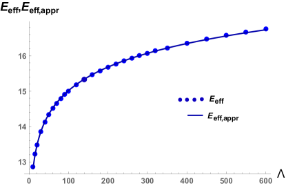
Figure 9: $E_{eff}$ as function of $\Lambda$ and its approximation $10.60+0.959\log x$.

6.3 Phase transition

To study the phase transition we consider the deformation of $\rho_{\sinh\sqrt{\lambda}}$ by $\rho_{\exp}$

$$\rho_{nn}(\lambda)=\rho_{\sinh\sqrt{\lambda}}(\lambda,\Lambda)+J\rho_{e^{w\lambda}}(\lambda,\Lambda,\omega)$$ (87)

It is interesting to compare this density with the density

$$\rho_{nn,s}(\lambda)=\rho_{\sinh\sqrt{\lambda(1-\lambda/\Lambda)}}(\lambda,\Lambda)+J\rho_{e^{w\lambda}}(\lambda,\Lambda,\omega),$$ (88)

where

$$\rho_{\sinh\sqrt{\lambda(1-\lambda/\Lambda)}}(\lambda,\Lambda)=\frac{n_{s}(\Lambda)}{(2\pi)^{2}}\sinh 2\pi\sqrt{\lambda(1-\lambda/\Lambda)}.$$ (89)

In Fig.10 we plot the density (87) and (88) for $\omega=-1$ and different $J$ and $\Lambda$. We see that for negative $J>J_{cr}(\Lambda)$ domains on the segment $0,\Lambda$, where $\rho_{nn}$ and $\rho_{nn,s}$ become negative, appear. We interpret this as a destruction of the solution, or in other words, as an appearance of a phase transition at $J_{cr}$. It is interesting that the critical value $J_{cr}$ are the same for both $\rho_{nn}$ and $\rho_{nn,s}$. In Fig.11 the locations of critical points depending on $\Lambda$ are shown.

In Fig.12 the dependence of $n(\Lambda)$ on $J$ for fixed $\Lambda$ and $\omega$ for different values of $\Lambda$ is shown. For (a),(b) and (c) these plots are for $\Lambda=5,7.5,10$. Here $J>J_{cr}(\Lambda)$. We see normalization factor increases with increasing $J$ and this dependence is linear. This dependence differs from the dependence for the Gaussian perturbed ensemble (see Fig.7.a), where it is given by a decreasing nonlinear function. The plot in Fig.12.b) shows the dependence of critical current $J_{cr}$ on $n(\Lambda)$.

 

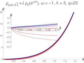
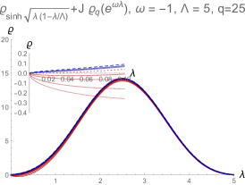
(a)                                                  (b)

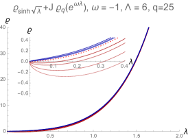
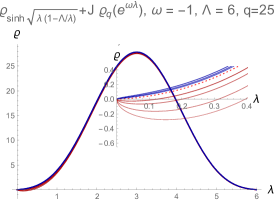
(c)                                                  (d)

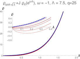
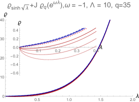
(e)                                                  (f)

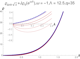
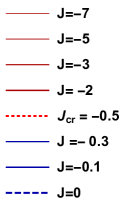
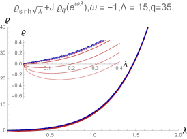
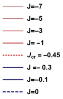
(i)                                                  (j)

Figure 10: The plots of density (87) for $\Lambda=5,6,7.5,10,12.5,15$ (a,c,e,f,i,j) and density (88) for $\Lambda=5,6$ (b,d). In all cases $\omega=-1$. Legends in (a,b), and (c,d) are the same.

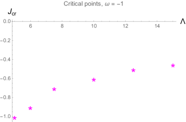
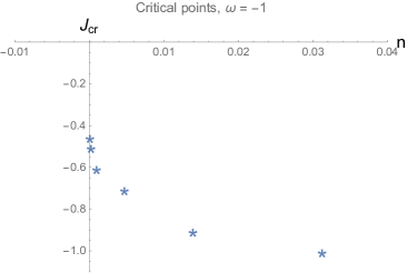
Figure 11: (a) The points show the values of $J_{cr}$ for $\rho(\lambda)$ given by (87) for different $\Lambda$. (b) $J_{cr}$ vs normalization $n(\Lambda)$ for the same $\Lambda$ as at (b). $\omega=-1$.

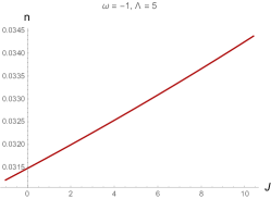
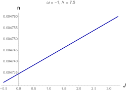
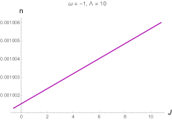
Figure 12: Relations between $n(\Lambda)$, normalization factor, and $J$ for fixed $\Lambda$ for $\rho(\lambda)$ given by (87). The lines start at the points presented at Fig.11.a.

7 Discussion and conclusion

The generating functional for the correlation functions of the boundaries of the Riemann serfaces is considered in JT gravity and in matrix theory. The matrix integral SSS provides a nonperturbative completion of the genus expansion in JT gravity on Riemann surfaces with fixed number of boundaries for all genus. The generating functional ${\mathfrak{Z}}(J)$ considered in this paper, gives completion also for infinitely many number of boundaries.

By using this formulation with several matrix models, including double scaling limit for the Gaussian model, relevant to topological gravity, cubic model, and JT gravity have been investigated. In all these cases (here we have presented only results for topological and JT gravities), in the corresponding gas of baby universes the phase transition is observed. By analogy with states of matter one could expect that this phase change is condensation from the gaseous state of JT multiverse to liquid state.

To study this phase transition, we consider generating functional that we associate with baby universes. The generating functional for a matrix model with potential $V(x)$ is obtained from the partition function of the model just by shift $V(x)\to V(x)-\widetilde{J}(x)$ where $\widetilde{J}(x)$ is the Laplace transform of $J(\beta)$. Baby universes should look as point-like objects with very small length of the boundary. Therefore the distribution $J(\beta)$ should have a peak somewhere near zero. In our model with $J(\beta)=J\delta(\beta-\omega)$ baby universes correspond to small $\omega$. The shifted potential in this case is $V(x)-Je^{-\omega x}$. Note that one could expect $<Z(\beta)^{n}>\approx<Z(\beta)>^{n}$ for large $n$ similarly to the infinite replica number limit considered in AKTV .

We have obtained that in all cases there are critical negative $J_{cr}$, such that for $J<J_{cr}$ the corresponding solution is destroyed. The mass at the critical points decreases with increasing of $\Lambda$. In this paper we have considered the deformation of the density function by the exponential potential, but is also possible to study all momenta deformations, as well as $\det(E-M)$, compare with Garc a .

The holographic boundary dual of the JT gravity in spacetime with $M$ boundaries is the $M$-replica SYK model in the low energy limit Jensen:2016pah ; Maldacena:2016upp ; Engelsoy:2016xyb ; Harlow . The studies of AV ; AKTV ; Kamenev ; 1902.09970 ; Okuyama:2019xvg ; AKV show that the nonperturbative completion of SYK involves nontrivial replica-nondiagonal saddle points. The replica-nondiagonal structures in SYK with replica interaction 1804.00491 ; 1901.06031 ; Klebanov ; AKV demonstrate nontrivial phase structures and symmetry breaking patterns.

Note that the deformation of potential by the linear term or nonlinear ones as a tool for investigation of phase transitions and spontaneous symmetry breaking in SYK-like models was used in AV ; 1902.09970 ; AKV . In particular, a nonlocal interacting of two-replica by a nonlocal term proportional to an external current permits to reveal nonperturbative effects in the SYK model. This nonlocality in some sense is analogous to an external nonlocal source $J(x)$ (cosmological daemon) in cosmology 1103.0273 , there it specified boundary conditions.

There are numerous investigations of wormholes and baby universes in cosmology and particle physics, including the Giddings–Strominger wormhole solution GS and Coleman’s approach to the cosmological constant problem Coleman . There are many open questions in theory of wormholes and baby universes. In particular, it would be interesting to see whether in JT gravity or its generalizations there is a mechanism of suppression CK the probability of creation of giant wormholes and big baby universes. By using the wormhole/baby universe approach it was found that the probability for the universe to undergo a spontaneous compactification down to a four-dimensional spacetime is greater than to remain in the original homogeneous multidimensional state IV . It is interesting to find an analog of this in the context of JT gravity.

In the study of SYK from gravity perspective, a crutial role plays consideration of wormholes in JT gravity 1804.00491 ; 1904.01911 ; 1904.12820 ; 1903.10532 ; 1903.05732 ; 1903.05658 ; 1901.06031 . A interplay between baby universes and wormholes could lead to nontrivial effects.

Using the recent result of 1905.03780 according which JT gravity in $dS_{2}$ is an analytic continuation of JT gravity in Euclidean $AdS_{2}$ it would be interesting to understand the meaning of the phase transition considered here in the dS case.

It would be also interesting to to compare the Hartle-Hawking construction of string baby universes related with $AdS_{2}\times S^{2}$ geometry, using free fermionic formulation Dijkgraaf:2005bp with the fermionic interpretation of determinant in matrix models, and also find a slot for baby universes in an quasi-classical 1812.00918 ; 1902.11194 or exact quantization of JT proposed in 1905.02726 .

References

- (1) P. Saad, S. H. Shenker and D. Stanford, “JT gravity as a matrix integral,” arXiv:1903.11115.
- (2) R. Jackiw, “Lower Dimensional Gravity,” Nucl. Phys. B252 (1985) 343–356.
- (3) C. Teitelboim, “Gravitation and Hamiltonian Structure in Two Space-Time Dimensions,” Phys. Lett. B126 (1983) 41–45.
- (4) M. Mirzakhani, “Growth of Weil-Petersson volumes and random hyperbolic surface of large genus,” Journal of Differential Geometry, 94 (2013) 267–300.
- (5) B. Eynard and N. Orantin, “Invariants of algebraic curves and topological expansion,” arXiv:math-ph/0702045.
- (6) B. Eynard and N. Orantin, “Weil-Petersson volume of moduli spaces, Mirzakhani’s recursion and matrix models,” arXiv:0705.3600 [math-ph].
- (7) E. Witten, “Two-dimensional gravity and intersection theory on moduli space,” Surveys Diff. Geom. 1 (1991) 243–310.
- (8) M. Kontsevich, “Intersection theory on the moduli space of curves and the matrix airy function,” Comm. Math. Phys.147 (1992)1-23.
- (9) Y. I. Manin and P. Zograf, “Invertible Cohomological Field Theories and Weil-Petersson volumes”, arXiv: math/9902051
- (10) R. Dijkgraaf and E. Witten, “Developments in Topological Gravity,” arXiv:1804.03275
- (11) J. S. Cotler, G. Gur-Ari, M. Hanada, J. Polchinski, P. Saad, S. H. Shenker, D. Stanford, A. Streicher, and M. Tezuka, “Black Holes and Random Matrices,” JHEP 05 (2017)118, arXiv:1611.04650.
- (12) P. Saad, S. H. Shenker, and D. Stanford, “A semiclassical ramp in SYK and in gravity,” arXiv:1806.06840.
- (13) M.B. Green, J.H. Schwarz, E. Witten, Superstring Theory, Cambridge, UK: Univ. Press. ( 1987) 469 pp
- (14) E. Witten, “Noncommutative Geometry and String Field Theory,” Nucl. Phys. B 268 (1986) 253.
- (15) I.Ya. Aref’eva and I.V. Volovich, Two-dimensional gravity, string field theory and spin glasses, Phys.Lett. 255 (1991) 197-201
- (16) E.P. Wigner, Proc. Cambridge Philos. Soc. 47 (1951) 790, reprinted in C.E. Porter, Statistical theories of spectra: fluctuations (Academic Press, New York, 1965)
- (17) F. J. Dyson, A Class of Matrix Ensembles, J. Math. Phys. 13 (1972) 90.
- (18) E. Brezin, C. Itzykson, G. Parisi and J.-B. Zuber, Commun. Math. Phys. 50 (1978) 35
- (19) M.L. Mehta, Random matrices, 2nd edition, Academic Press, New York, 1991.
- (20) N.I. Muskhelishvili, Singular integral equations, Noordhoff, 1953.
- (21) F.D. Gakhov, Boundary problems, Fizmatgiz, Moscow, 1977 [in Russian].
- (22) E. Brézin and V. A. Kazakov, “Exactly Solvable Field Theories Of Closed Strings,” Phys. Lett. B 236 (1990) 144.
- (23) M. R. Douglas and S. H. Shenker, “Strings In Less Than One-Dimension,” Nucl. Phys. B 335 (1990) 635.
- (24) D. J. Gross and A. A. Migdal, “Nonperturbative Two-Dimensional Quantum Gravity,” Phys. Rev. Lett. 64 (1990) 127 .
- (25) P. Di Francesco, P. Ginsparg and J. Zinn-Justin, “2-D Gravity and random matrices,” Phys. Rept. 254 (1995) 1, arXiv:hep-th/9306153.
- (26) M. Marino, “Les Houches lectures on matrix models and topological strings,” hep-th/0410165.
- (27) B. Eynard, T. Kimura and S. Ribault, “Random matrices,” arXiv:1510.04430 [math-ph].
- (28) A. Migdal, “Loop equations and expansion,” Phys. Rept. 102 (1983) 199.
- (29) J. Ambjorn, J. Jurkiewicz and Yu. M. Makeenko, ”Multiloop correlators for two-dimensional quantum gravity,” Phys. Lett. B251 (1990) 517
- (30) B. Eynard, “Topological expansion for the 1-Hermitian matrix model correlation functions,” JHEP 0411, 031 (2004), arXiv:hep-th/0407261.
- (31) A. Almheiri and J. Polchinski, “Models of AdS2 backreaction and holography,” JHEP, 11 (2015) 014, arXiv:1402.6334 [hep-th].
- (32) S W Hawking, Phys Lett B195 (1987) 337
- (33) S W Hawkang and R Laflamme, Baby universes and the non-renormalizability of gravity, Phys.Lett.209 (1988), 39-41
-
(34)
G. V. Lavrelashvili, V. A. Rubakov, and P. G. Tinyakov, “Disruption of
Quantum Coherence upon a Change in Spatial Topology in Quantum Gravity,”
JETP Lett 46 (1987) 167
G. V. Lavrelashvili, V. A. Rubakov, and P. G. Tinyakov, Nuel. Phys. B 290 (1988) 757 - (35) S. B. Giddings and A. Strominger, “Axion Induced Topology Change in Quantum Gravity and String Theory,” Nucl. Phys. B306 (1988) 890–907.
- (36) S. B. Giddings and A. Strominger, “Baby Universes, Third Quantization and the Cosmological Constant,” B321 (1989) 481–508.
- (37) A. Strominger, Baby Universes, In: ”Quantum Cosmology and Baby Universes”, (1991) pp. 269-346.
- (38) S. R. Coleman, “Why There Is Nothing Rather Than Something: A Theory of the Cosmological Constant,” Nucl. Phys. B 310 (1988) 643.
- (39) I. V. Volovich, ”Baby universes and the dimensionality of spacetime”, Phys. Lett. B, 219 (1989), 66-70.
- (40) A. Hebecker, T. Mikhail and P. Soler, “Euclidean wormholes, baby universes, and their impact on particle physics and cosmology,” Front. Astron. Space Sci. 5 (2018) 35 , arXiv:1807.00824.
- (41) S. Jain and S. D. Mathur, “World sheet geometry and baby universes in 2-D quantum gravity,” Phys. Lett. B 286 (1992) 239, hep-th/9204017.
- (42) J. Ambjorn, J. Barkley, T. Budd and R. Loll, “Baby Universes Revisited,” Phys. Lett. B 706 (2011) 86, arXiv:1110.3998.
- (43) E. Brezin and A. Zee, “Universality of the correlations between eigenvalues of large random matrices,” Nucl. Phys. B 402 (1993) 613.
- (44) M. Bowick and E. Brezin, ”Universal scaling of the tail of the density of eigenvalues in random matrix models,” Phys. Lett B268 (1991) 21
- (45) Pavel Bleher, Alexander Its, ”Double scaling limit in the random matrix model: the Riemann-Hilbert approach”, Comm. on Pure and Applied Math., Vol.56, Issue 4 (2003), doi.org/10.1002/cpa.10065; arXiv:math-ph/0201003
-
(46)
A. Boutet de Monvel, L. Pastur, and M. Shcherbina. ”On the statistical mechanics approach in the random matrix theory: Integrated density of state”, J. Stat. Phys. 79 (1995) 585.
L. Pastur, and M. Shcherbina, ”Universality of the Local Eigenvalue Statistics for a Class of Unitary Invariant Random Matrix Ensembles”, J. Stat. Phys. Vol. 86, (1997), 109 -
(47)
C. Tracy and H. Widom, ”Level-Spacing Distributions and the Airy Kernel”, Commun.Math. Phys. 159 (1994) 151-174.
C. Tracy and H. Widom, ”Fredholm Determinants, Differential Equations and Matrix Models”, Commun. Math. Phys. 163:35 (1994) 33-72 - (48) A. B. J. Kuijlaars and K. T-R McLauglin, Generic behavior of the density of states in random matrix theory and equilibrium problems in the presence of real analytic external field, Commun. Pure Appl. Math. 53 (2000) 736-785.
- (49) P. Deift, T. Kriecherbauer, K. T-R. McLaughlin, S. Venakides, and X. Zhou, Uniform asymptotics for polynomials orthogonal with respect to varying exponential weights and applications to universality questions in random matrix theory, Commun. Pure Appl. Math., 52 (1999) 1335-1425 .
- (50) E. Brezin and S. Hikami, Random Matrix Theory with an External Source, doi:10.1007/978-981-10-3316-2
- (51) I.Ya. Arefeva, A.C. Ilchev and B.K. Mitruchkin, ”Phase structure of matrix NxN Goldstoune model in the large N limit”, In: Proceedings of ”III international Symposium on selected topics in statistical mechanics”, Dubna 22-26 August, 1984; preprint JINR D17-84-850, p.20-26.
- (52) G. M. Cicuta, L. Molinari, and Montaldi, Large phase transition in low dimensions, Mod. Phys. Lett. A1 (1986) 125.
- (53) C. Crnkovic and G. Moore, Multicritical multi-cut matrix models, Phys. Lett. B 257 (1991).
- (54) V.A. Kazakov, A simple solvable model of quantum field theory of open strings, Phys.Lett.B. 237 (1990), 212-216
- (55) D. Bagrets, A. Altland, A. Kamenev, ”Sachdev-Ye-Kitaev Model as Liouville Quantum Mechanics”, Nucl. Phys. B 911 (2016) 191-205, arXiv:1607.00694
- (56) D. Stanford and E. Witten, “Fermionic Localization of the Schwarzian Theory,” JHEP 10 (2017) 008, arXiv:1703.04612.
- (57) H. A. Bethe, ”An Attempt to Calculate the Number Energy Levels of a Heavy Nucleus”, Phys.Rev., 50 (1936) 332
- (58) A. M. Garcia-Garcia, Y. Jia and J. J. M. Verbaarschot, “Exact moments of the Sachdev-Ye-Kitaev model up to order ,” JHEP 1804 (2018) 146, arXiv:1801.02696.
- (59) K. Jensen, “Chaos in AdS2 Holography,” Phys. Rev. Lett. 117, no. 11, 111601 (2016) arXiv:1605.06098
- (60) J. Engels y, T. G. Mertens, and H. Verlinde, “An investigation of AdS2 backreaction and holography,” JHEP 07 (2016) 139, arXiv:1606.03438 [hep-th].
- (61) J. Maldacena, D. Stanford, and Z. Yang, “Conformal symmetry and its breaking in two dimensional Nearly Anti-de-Sitter space,” PTEP 12, (2016) 12C10, arXiv:1606.01857.
- (62) D. Harlow and D. Jafferis, “The Factorization Problem in Jackiw-Teitelboim Gravity,” arXiv:1804.01081.
- (63) J. Maldacena, X.-L. Qi, ”Eternal traversable wormhole”, arXiv:1804.00491
- (64) I. Aref’eva and I. Volovich, “Notes on the SYK model in real time,” Theor. Math. Phys. 197 (2018) 1650 arXiv:1801.08118.
- (65) I. Aref’eva and I. Volovich, “Spontaneous symmetry breaking in fermionic random matrix model,” arXiv:1902.09970.
- (66) K. Okuyama, “Replica symmetry breaking in random matrix model: a toy model of wormhole networks,” arXiv:1903.11776 [hep-th].
- (67) I. Aref’eva, M. Khramtsov, M. Tikhanovskaya and I. Volovich, “Replica-nondiagonal solutions in the SYK model,” arXiv:1811.04831 [hep-th].
- (68) H. Wang, D. Bagrets, A. L. Chudnovskiy and A. Kamenev, ”On the replica structure of Sachdev-Ye-Kitaev model,” arXiv:1812.02666 [hep-th].
- (69) I.Ya. Aref’eva, I.V. Volovich, Cosmological daemon, JHEP, 8 (2011) 102, arXiv: 1103.0273
- (70) S.R. Coleman, Ki-Myeong Lee, Escape From the Menace of the Giant Wormholes, Phys.Lett. B221 (1989) 242-249.
- (71) J. Kim, I. R. Klebanov, G. Tarnopolsky and W. Zhao, ”Symmetry Breaking in Coupled SYK or Tensor Models,” arXiv:1902.02287 .
- (72) I. Aref’eva, M. Khramtsov and I. Volovich, “Revealing nonperturbative effects in the SYK model,” arXiv:1905.04203 [hep-th].
- (73) J. Maldacena, G. J. Turiaci, Zh. Yang, ”Two dimensional Nearly de Sitter gravity”, arXiv:1904.01911
- (74) H. W. Lin, J. Maldacena, Ying Zhao, ”Symmetries Near the Horizon”, arXiv:1904.12820
- (75) Y. Chen, P. Zhang, ”Entanglement Entropy of Two Coupled SYK Models and Eternal Traversable Wormhole”, arXiv:1903.10532
- (76) B. Freivogel, V. Godet, Ed. Morvan, J. F. Pedraza, A. Rotundo ”Lessons on Eternal Traversable Wormholes in AdS”, arXiv:1903.05732
- (77) P. Betzios, E. Kiritsis, O. Papadoulaki, Euclidean Wormholes and Holography, arXiv:1903.05658
- (78) A. M. Garci a-Garcia, T. Nosaka, D. Rosa, J. J. M. Verbaarschot, Quantum chaos transition in a two-site SYK model dual to an eternal traversable wormhole, arXiv:1901.06031
- (79) J. Cotler, K. Jensen, A. Maloney, Low-dimensional de Sitter quantum gravity, arXiv:1905.03780
- (80) R. Dijkgraaf, R. Gopakumar, H. Ooguri and C. Vafa, “Baby universes in string theory,” Phys. Rev. D 73 (2006) 066002, hep-th/0504221.
- (81) A. Blommaert, T. G. Mertens and H. Verschelde, ”Fine Structure of Jackiw-Teitelboim Quantum Gravity,” arXiv:1812.00918 .
- (82) A. Blommaert, T. G. Mertens and H. Verschelde, ”Clocks and Rods in Jackiw-Teitelboim Quantum Gravity,” arXiv:1902.11194.
- (83) L. V. Iliesiu, S. S. Pufu, H. Verlinde, Y. Wang, An exact quantization of Jackiw-Teitelboim gravity, arXiv:1905.02726