A Bayesian Approach to Robust Reinforcement Learning

Abstract

Robust Markov Decision Processes (RMDPs) intend to ensure robustness with respect to changing or adversarial system behavior. In this framework, transitions are modeled as arbitrary elements of a known and properly structured uncertainty set and a robust optimal policy can be derived under the worst-case scenario. In this study, we address the issue of learning in RMDPs using a Bayesian approach. We introduce the Uncertainty Robust Bellman Equation (URBE) which encourages safe exploration for adapting the uncertainty set to new observations while preserving robustness. We propose a URBE-based algorithm, DQN-URBE, that scales this method to higher dimensional domains. Our experiments show that the derived URBE-based strategy leads to a better trade-off between less conservative solutions and robustness in the presence of model misspecification. In addition, we show that the DQN-URBE algorithm can adapt significantly faster to changing dynamics online compared to existing robust techniques with fixed uncertainty sets.

1 INTRODUCTION

Markov Decisions Processes (MDPs) are used for solving sequential decision making problems with varying degrees of uncertainty. Two types of uncertainty are encountered: the internal uncertainty due to the stochasticity of the system and the uncertainty in the transition and reward parameters [Mannor et al., 2007]. In order to mitigate the second type of uncertainty, the Robust-MDP (RMDP) framework considers the unknown parameters to be a member of a known uncertainty set [Nilim and El Ghaoui, 2005; Iyengar, 2005; Wiesemann et al., 2013]. An optimal solution to the robust RL problem then corresponds to the strategy that maximizes the worst-case performance and it can be derived using dynamic programming [Iyengar, 2005; Tamar et al., 2014].

However, planning in RMDPs often leads to overly conservative solutions. There are two reasons for this: Firstly, the uncertainty set has to be rectangular in order for the problem to be computationally tractable, which means that it must be structured as sets of MDP models that are independent for each state [Wiesemann et al., 2013]. Let give an intuition of the reason why the resulting policy may be too conservative. Suppose a chess player wants to protect himself against an adversary he has some prior on, which can be modeled as a set of transition models. Suppose also that the agent optimizes its next move according to the worst-case scenario from the set of models. Then, the rectangularity assumption implies that the agent considers the worst-case transition for each game configuration independently, although there are several chances that some configurations are incompatible during the same round of game. It comes out that this robust strategy is overly conservative. Attempts to circumvent rectangular uncertainty sets in RMDPs include the works [Mannor et al., 2012, 2016; Tirinzoni et al., 2018] and more recently, [Goyal and Grand-Clement, 2019].

Secondly, the difficulty of constructing uncertainty sets can result in too large sets and consequently lead to overly-pessimistic strategies [Petrik and Russell, 2019]. Proposals for learning an uncertainty set in a data-driven manner have rarely been addressed in RL literature. In [Petrik and Russell, 2019], the authors designed a robustification procedure that builds safe uncertainty sets upon optimal value functions. Their Bayesian method starts from a posterior distribution on transitions and constructs possibly discontinuous sets by iteratively solving optimization problems. Although it leads to tighter uncertainty sets, their algorithm proceeds offline with a fixed batch of data and is not scalable due to its high computational complexity. Moreover, their technique assumes the data to be generated by one fixed but unknown model, so it has not been tested against changing dynamics.

Previous work [Lim et al., 2016b] has used the “optimism in face of uncertainty” (OFU) principle [Jaksch et al., 2010] to detect adversarial state-action pairs online and compute an optimistic minimax policy accordingly. Although these methods have been proven to be statistically efficient, they require an exhaustive computation for each state-action pair. This leads to solutions that are intractable for all but small problems. Also, as is common in optimistic approaches, the resulting performance is highly influenced by the underlying analysis [Osband et al., 2013].

Based on a Bayesian approach, Thompson sampling [Thompson, 1933] has been shown to be more efficient than OFU methods in RL problems. Previous work [Osband and Van Roy, 2017] has stressed the advantages of posterior sampling methods over existing algorithms driven by optimism. However, most of the existing work on posterior sampling methods studied finite tabular MDPs. The Uncertainty Bellman Equation (UBE) work [O’Donoghue et al., 2018] addressed this shortcoming and proposed an online algorithm that scales naturally to large domains. Their method learns the posterior variance of the value for guiding exploration when the true dynamics of the MDP are unknown. Yet, their approach does not deal with adversarial transitions. While better exploration can potentially lead to more efficient learning and improved solutions, it cannot protect itself against sudden (potentially) adversarial changes in the underlying dynamics of the environment. This is especially true when the domain is large and/or hard to explore efficiently.

In this work, we introduce a Bayesian framework for robust RL and address the first Bayesian algorithm that (1) accounts for changing dynamics online and (2) tackles conservativeness thanks to a variance bonus that detects changes in the level of adversity. This variance is proven to satisfy an Uncertainty Robust Bellman Equation (URBE), that is estimated using dynamic programming. Besides being scalable to complex domains, our approach leads to less conservative results than existing planning methods for RMDPs while ensuring robustness to model misspecification . Our experiments illustrate an improved trade-off between overly conservative, robust behaviour and less conservative, improved performance for the resulting DQN-URBE policy.

Main Contributions: To summarize, our specific contributions are: (1) The URBE which encourages safe exploration and prevents overly conservative solutions; (2) The DQN-URBE which scales and utilizes URBE to learn less conservative solutions that are still robust to model misspecification; (3) Adaptability of DQN-URBE to changing dynamics online.

2 BACKGROUND

Bayesian Reinforcement Learning Bayesian RL leverages methods from Bayesian inference to incorporate prior information about the Markov model into the learning process. Model-based Bayesian RL [Dearden et al., 1999; Strens, 2000; Osband et al., 2013] express prior information on parameters of the Markov process instead. In the work [Dearden et al., 1998], the authors introduced Bayesian Q-learning to learn the posterior distribution of the Q-values in the model-free setting. One major advantage of Bayesian RL is that it can benefit from prior information on the problem to tackle the exploration-exploitation dilemma (see [Ghavamzadeh et al., 2015] for a full review).

Robust MDP A robust MDP is a tuple $\langle\mathcal{S},\mathcal{A},r,\mathcal{P}\rangle$ where $\mathcal{S}$ and $\mathcal{A}$ respectively denote state and action spaces. The mapping $r:\mathcal{S}\times\mathcal{A}\rightarrow\mathbb{R}$ defines the immediate bounded reward function and $\mathcal{P}$ is a set of transition matrices that models the ambiguity in the transition distributions. As common in the robust RL literature, we assume $\mathcal{P}$ to be structured as a cartesian product $\bigotimes_{s\in\mathcal{S},a\in\mathcal{A}}\mathcal{P}_{s,a}$, which is also known as the state-action rectangularity assumption [Wiesemann et al., 2013]. In RMDPs, this implies that the nature can choose the worst-transition independently for each state and action.

Robust DQN The DQN algorithm uses a neural network as a function approximation of the Q-value and learns its parameters by optimizing a TD-loss. Similarly, the robust Bellman equation uses a robust TD-error as a loss criterion for learning a minimax policy [Roy et al., 2017]. In [Di-Castro Shashua and Mannor, 2017], a robust counterpart to DQN called RTD-DQN has been introduced and shown to be robust to model misspecification.

3 ROBUST MARKOV DECISION PROCESSES

We consider a robust MDP $\langle\mathcal{S},\mathcal{A},r,\mathcal{P}\rangle$ of finite state and action spaces, where each episode has finite horizon length $H\in\mathbb{N}$. At step $h$, an agent is in state $s^{h}$, selects an action $a^{h}$ according to a stochastic policy $\pi^{h}:\mathcal{S}\rightarrow\Delta_{\mathcal{A}}$ that maps each state to a probability distribution over the action space, $\Delta_{\mathcal{A}}$ denoting the set of distributions over $\mathcal{A}$. Thus, for all steps $h=1,\cdots,H$, $\sum_{a\in\mathcal{A}}\pi_{sa}^{h}=1$. After choosing an action, the agent gets a deterministic reward $r^{h}$ bounded by $R_{\max}$, and transitions to state $s^{h+1}$ according to an arbitrary transition $p_{s^{h},a^{h}}\in\mathcal{P}_{s^{h},a^{h}}$ which we will rather write as $p_{sa}^{h}\in\mathcal{P}_{sa}^{h}$ with a slight abuse of notation.

The robust action-value (or robust Q-value) at step $h$, state $s$, action $a$ and under policy $\pi:=(\pi^{1},\cdots,\pi^{H})$ is the expected discounted return under the worst-case scenario resulting from taking action $a$ at $s$ and following policy $\pi$ thereafter:

$$Q_{sa}^{h}:=\inf_{p\in\mathcal{P}}\mathbb{E}\left[\sum_{l=h}^{H}\gamma^{l-h}r^{l}\mid s^{h}=s,a^{h}=a,\pi,p\right],$$

with $\gamma\in(0,1]$. Likewise, the robust value at state $s$ under policy $\pi$ is $V^{h}(s):=\mathbb{E}_{a\sim\pi_{s}^{h}}[Q_{sa}^{h}]$. When it is clear from the context, we suppress the dependence on $\pi$ for notational convenience.

A robust optimal policy is derived by maximizing the expected worst-case discounted return:

$$J(\pi):=\inf_{p\in\mathcal{P}}\mathbb{E}^{\pi,p}\left[\sum_{h=1}^{H}\gamma^{h-1}r^{h}\right]=V^{1}(s).$$

Assuming a rectangular structure on $\mathcal{P}$, the robust Bellman operator $\mathcal{T}^{h}$ for policy $\pi$ at step $h$ relates the robust value at $h$ to the robust value at following steps [Nilim and El Ghaoui, 2005]:

$$\mathcal{T}^{h}Q_{sa}^{h+1}=r_{sa}^{h}+\gamma\inf_{p\in\mathcal{P}}\sum_{s^{\prime}\in\mathcal{S},a^{\prime}\in\mathcal{A}}\pi_{s^{\prime}a^{\prime}}^{h}p_{sas^{\prime}}^{h}Q_{s^{\prime}a^{\prime}}^{h+1},$$

where $r_{sa}^{h}$ denotes the immediate reward at step $h$ while being in state $s$ and executing action $a$. Computing the second term in the robust Bellman operator amounts to solving a robust optimization problem where the robust constraints are given by $\mathcal{P}$. In fact, the main challenge of robust optimization is to build an uncertainty set such that the solution stays tractable without being overly conservative.

4 THE UNCERTAINTY ROBUST BELLMAN EQUATION

In this section, we introduce our Bayesian framework for robust RL where we have a prior over the transition model. Our approach is based on the following procedures: (a) building posterior uncertainty sets, (b) approximating posterior distribution over robust Q-values. Next, we introduce an upper bound on the variance of the posterior over robust Q-values and show that it satisfies a Bellman recursion, which we call the Uncertainty Robust Bellman Equation (URBE). Proofs are deferred to the Appendix.

4.1 POSTERIOR UNCERTAINTY SETS

Define $\varphi_{p}$ as a prior distribution according to which state transitions are generated. Assume furthermore that $\varphi_{p}$ is a product of $|\mathcal{S}|\cdot|\mathcal{A}|$ independent Dirichlet priors on each distribution $p_{sa}$ over next states, that is $\varphi_{p}=\prod_{s,a}\varphi_{sa}$, where $\varphi_{sa}$ is Dirichlet. Given an observation history $\mathcal{H}=\langle(s_{1},a_{1}),(s_{2},a_{2}),\dots,(s_{h},a_{h})\rangle\in(\mathcal{S}\times\mathcal{A})^{h}$ induced by a policy $\pi$ and a confidence level $\psi_{sa}\in\mathbb{R}^{+}$ for each state-action pair, we can construct a subset of transition probabilities $\Delta_{\mathcal{S}}$:

$$\begin{split}\widehat{\mathcal{P}}^{h}_{sa}(\psi_{sa})=\left\{p_{sa}\in\Delta_{\mathcal{S}}:\lVert p_{sa}-\bar{p}_{sa}\rVert_{1}\leq\psi_{sa}\right\}\end{split}$$

where $\bar{p}_{sa}$ is the nominal transition given by $\bar{p}_{sa}=\mathbb{E}[p_{sa}\mid\mathcal{H}]$. If $\mathcal{H}$ is fixed, this construction falls into the definition of a Bayesian confidence interval introduced in [Petrik and Russell, 2019].

Such a construction forms a rectangular uncertainty set $\widehat{\mathcal{P}}^{h}(\psi):=\bigotimes_{s,a}\widehat{\mathcal{P}}^{h}_{sa}(\psi_{sa})$ We call it a posterior uncertainty set and will omit the dependence in $\psi$ for ease of notation. To derive smaller posterior regions of posterior confidence level $\alpha$, one can proceed as described in [Petrik and Russell, 2019; Gupta, 2018] by minimizing $\mathbb{P}(\lVert p_{sa}-\bar{p}_{sa}\rVert_{1}>\psi_{sa}\mid\mathcal{H})<\frac{\alpha}{|\mathcal{S}||\mathcal{A}|}$ with respect to $\psi_{sa}$ that satisfies the constraint. However, in our case, the data set is not fixed so the nominal transition changes, which raises tractability issues. Therefore, $\psi_{sa}$ is remained fixed without being optimized.

4.2 POSTERIOR OVER ROBUST Q-VALUES

The simulation proceeds as follows: at each episode $t$, we sample a transition matrix according to $\varphi_{p}$. For a fixed policy $\pi$, we collect observation history and update the posterior distribution accordingly. We then construct a posterior uncertainty set $\widehat{\mathcal{P}}^{h}_{sa}(\psi_{sa})$ based on all observed data from all previous episodes. A posterior over robust Q-values can then be obtained via the following equation:

$$\begin{split}\widehat{Q}_{sa}^{h}&=r_{sa}^{h}+\gamma\inf_{p\in\widehat{\mathcal{P}}_{sa}^{h}}\sum_{s^{\prime},a^{\prime}}\pi_{s^{\prime}a^{\prime}}^{h}p_{sas^{\prime}}\widehat{Q}_{s^{\prime}a^{\prime}}^{h+1}\enspace,\end{split}$$

with $\widehat{Q}_{sa}^{H+1}=0$. The quantity $\widehat{Q}_{sa}^{h}$ is a random variable whose variability comes from the nominal transition used in constructing posterior uncertainty sets, from the stochasticity of the policy and the dynamics of the sampled MDP. We further define

$$\begin{split}\widehat{p}_{sa}^{h}&\in\arg\min_{p\in\widehat{\mathcal{P}}_{sa}^{h}}\sum_{s^{\prime},a^{\prime}}\pi_{s^{\prime}a^{\prime}}^{h}p_{sas^{\prime}}\widehat{Q}_{s^{\prime}a^{\prime}}^{h+1}\end{split}$$ (1)

as a worst-case transition at step $h$.

4.3 POSTERIOR VARIANCE OF ROBUST Q-VALUES

For the regular MDP setting, the work [O’Donoghue et al., 2018] showed that the conditional variance of posterior Q-values can be bounded by a quantity that satisfies a Bellman recursion formula. In Bayesian robust RL, a similar upper bound by a robust Bellman update can be derived. The key difference with [O’Donoghue et al., 2018] is that they evaluate posterior Q-values according to one transition model whereas we evaluate robust Q-values according to a posterior uncertainty set.

Let first introduce some notation:

Notation 4.1.

Define $\mathcal{F}_{t}$ as a minimal sigma-algebra that contains all of the available information up to episode $t$ (e.g. all observed states, actions and rewards). Denote by $\mathbb{E}_{t}[X]$ the expectation of random variable $X$ conditioned on $\mathcal{F}_{t}$. Similarly, the conditional variance $\mathbf{var}_{t}(X)$ is defined as: $\mathbf{var}_{t}X:=\mathbb{E}_{t}\left[\left(X-\mathbb{E}_{t}[X]\right)^{2}\right]$.

As common in literature [Osband et al., 2016; O’Donoghue et al., 2018], we make the following assumptions:

Assumption 4.1.

For any episode, the graph resulting from a worst-case transition model is directed and acyclic.

Assumption 4.2.

For all $(s,a)\in\mathcal{S}\times\mathcal{A}$, the rewards are bounded: $-R_{\max}\leq r_{sa}\leq R_{\max}$. This implies that the robust Q-value is bounded as well: $\mid Q_{sa}^{h}\mid\leq HR_{\max}=:Q_{\max}$.

These assumptions enable to state the following result.

Lemma 4.1.

Under Assumptions 4.1 and 4.2, for any worst-case transition $\widehat{p}$ as defined in equation (1), the conditional variance of the robust Q-values under the posterior distribution satisfies the robust Bellman inequality:

$$\mathbf{var}_{t}\widehat{Q}_{sa}^{h}\leq\nu_{sa}^{h}+\gamma^{2}\sum_{s^{\prime},a^{\prime}}\pi_{s^{\prime}a^{\prime}}^{h}\mathbb{E}_{t}\left(\widehat{p}_{sas^{\prime}}^{h}\right)\mathbf{var}_{t}\widehat{Q}_{s^{\prime}a^{\prime}}^{h+1},$$

with $\mathbf{var}_{t}\widehat{Q}^{H+1}=0$ and $\nu_{sa}^{h}:=Q^{2}_{\max}\sum_{s^{\prime}\in\mathcal{S}}\frac{\mathbf{var}_{t}\widehat{p}_{sas^{\prime}}^{h}}{\mathbb{E}_{t}\widehat{p}_{sas^{\prime}}^{h}}$.

This lemma enables us to establish the Uncertainty Robust Bellman Equation (URBE).

Theorem 4.1 (Solution of URBE).

For any worst-case transition $\widehat{p}$ as defined in equation (1) and any policy $\pi$, under Assumptions 4.1 and 4.2, there exists a unique mapping $w$ that satisfies the uncertainty robust Bellman equation:

$$w_{sa}^{h}=\nu_{sa}^{h}+\gamma^{2}\sum_{s^{\prime}\in\mathcal{S},a^{\prime}\in\mathcal{A}}\pi_{s^{\prime}a^{\prime}}^{h}\mathbb{E}_{t}(\widehat{p}_{sas^{\prime}}^{h})w_{s^{\prime}a^{\prime}}^{h+1},$$ (2)

for all $(s,a)\in\mathcal{S}\times\mathcal{A}$ and $h=1,\cdots,H$ where $w^{H+1}=0$. Furthermore, $w\geq\mathbf{var}_{t}\widehat{Q}$.

A classical difficulty in Bayesian approaches is to compute the posterior distribution. The Bayesian central limit theorem (Result 8 in [Berger, 2013]) ensures that under smoothness assumptions on the prior and likelihood functions, the posterior distribution converges to a Gaussian distribution. Thus, we get around tractability issues by approximating the posterior over robust Q-values as $\mathcal{N}(\bar{Q},\mathbf{diag}(w))$, where $w$ is the solution to URBE and $\bar{Q}$ is the unique solution to:

$$\begin{split}\bar{Q}_{sa}^{h}&=r_{sa}^{h}+\gamma\sum_{s^{\prime},a^{\prime}}\pi_{s^{\prime}a^{\prime}}^{h}\mathbb{E}_{t}(\widehat{p}_{sas^{\prime}}^{h})\bar{Q}_{s^{\prime}a^{\prime}}^{h+1},\end{split}$$

for $h=1,\cdots,H$, and $\bar{Q}^{H+1}=0$.

Remark 4.1.

We should emphasize that the quantity $\mathbb{E}_{t}(\widehat{p}_{sas^{\prime}}^{h})$ is the conditional expectation of the worst-case transition, and depends on the robust Q-values. Therefore, it is different from the nominal transition which only depends on observations.

5 ESTIMATION OF THE ROBUST LOCAL UNCERTAINTY

Lemma 4.1 reveals a quantity $\nu$ that only depends on local state and action pairs. We call it the robust local uncertainty, since it also depends on the worst-case transitions. In this section, we present a practical method for estimating this quantity, which will be useful for implementing learning algorithms that take advantage of Theorem 4.1. We first present the tabular representation in the robust setup. We then recall the linear function representation and neural network architectures from [O’Donoghue et al., 2018] which directly enable to scale up the robust local uncertainty estimate.

5.1 TABULAR CASE

Assume a Dirichlet prior $\varphi_{sa}:=(\varphi_{sas^{\prime}})_{s^{\prime}\in\mathcal{S}}$ on transitions that depart from $(s,a)\in\mathcal{S}\times\mathcal{A}$. For all $h=1,\cdots,H$, the posterior distribution is Dirichlet:

$$p_{sa}^{h}\mid\mathcal{F}_{t}\sim\text{Dir}(\varphi_{sa}+n_{sa}^{h})$$

where $n_{sa}^{h}:=(n_{sas^{\prime}}^{h})_{s^{\prime}\in\mathcal{S}}$ is the vector of counts for observation $(s,a,s^{\prime})$ at step $h$, up to episode $t$. Therefore, given a posterior uncertainty set $\widehat{\mathcal{P}}^{h}_{sa}$ at step $h$, any $p_{sa}^{h}\in\widehat{\mathcal{P}}^{h}_{sa}$ satisfies the following:

$$\mathbf{var}_{t}p_{sas^{\prime}}^{h}\leq\frac{\varphi_{sas^{\prime}}+n_{sas^{\prime}}^{h}}{\left(\sum_{s^{\prime}\in\mathcal{S}}(\varphi_{sas^{\prime}}+n_{sas^{\prime}}^{h})\right)^{2}},$$

$$\mathbb{E}_{t}p_{sas^{\prime}}^{h}=\frac{\varphi_{sas^{\prime}}+n_{sas^{\prime}}^{h}}{\sum_{s^{\prime}\in\mathcal{S}}(\varphi_{sas^{\prime}}+n_{sas^{\prime}}^{h})}.$$

Since $\widehat{\mathcal{P}}^{h}_{sa}$ is a closed set, $\widehat{p}_{sas^{\prime}}$ also satisfies these inequalities and

$$\frac{\mathbf{var}_{t}\widehat{p}_{sas^{\prime}}^{h}}{\mathbb{E}_{t}\widehat{p}_{sas^{\prime}}^{h}}\leq\frac{1}{\sum_{s^{\prime}\in\mathcal{S}}(\varphi_{sas^{\prime}}+n_{sas^{\prime}}^{h})}\leq\frac{1}{n_{sa}^{h}},$$

where $n_{sa}^{h}$ is the visit count of the agent from state $s$ and action $a$. It follows that $\nu_{sa}^{h}\leq Q^{2}_{\max}\mid S\mid/n_{sa}^{h}$. Therefore, similarly to the non-robust setup, the robust local uncertainty can be modeled as a positive constant $\beta^{2}$ divided by the visit count $n_{sa}^{h}$.

5.2 FUNCTION APPROXIMATION

We now adapt the robust local uncertainty estimate to function approximation representations. Let $\widehat{Q}_{sa}^{h}\approx\phi_{s}^{T}\theta_{a}$ be a linear function approximation for the robust Q-values, where $\phi:\mathcal{S}\rightarrow\mathbb{R}^{d}$ designates state features and $\theta_{a}$ are parameters learned for each action $a\in\mathcal{A}$. Using the inverse count estimator $(\widehat{n}_{sa}^{h})^{-1}=\phi_{s}^{T}(\Phi_{a}^{T}\Phi_{a})^{-1}\phi_{s}$ introduced in the work [O’Donoghue et al., 2018], where $\Phi_{a}$ is the matrix of $\phi_{s}$-s stacked row-wise with action $a$ being taken at $s$, we estimate the robust local uncertainty by $\widehat{\nu}_{sa}^{h}=\beta^{2}\phi_{s}^{T}(\Phi_{a}^{T}\Phi_{a})^{-1}\phi_{s}$. As it receives a new sample $\phi$, the agent needs to update the matrix $\Sigma_{a}:=(\Phi_{a}^{T}\Phi_{a})^{-1}$, which can be implemented efficiently via the Sherman-Morrison-Woodbury formula [Golub and Van Loan, 1996]:

$$\Sigma_{a}^{+}:=\Sigma_{a}-(\Sigma_{a}\phi\phi^{T}\Sigma_{a})/(1+\phi^{T}\Sigma_{a}\phi).$$ (3)

The neural network representation proceeds similarly, provided that we treat all layers as feature extractors and apply a linear activation function to the last layer. In that case, we still have $\widehat{Q}_{sa}^{h}\approx\phi_{s}^{T}\theta_{a}$, where $\phi_{s}$ is the output of the last network layer for state $s$ and $\theta_{a}$ are the parameters of the last layer for action $a$. We use this technique in Algorithm 2.

6 URBE-BASED ALGORITHMS

6.1 URBE ALGORITHM

The URBE algorithm is described in Algorithm 1. Its structure is similar to [Osband et al., 2013], but involves using robust dynamic programming so as to learn a robust policy as well as posterior variance of the robust Q-values. At the beginning of each episode, an MDP model is sampled according to the current posterior distribution. The posterior uncertainty set is also updated according to new observations. Robust Q-values and its posterior variance are then computed using dynamic programming. At each step, the agent acts greedily with respect to the robust Q-values plus the posterior variance.

Algorithm 1 URBE

  Input: Prior distribution $\phi_{p}$, confidence level $\psi$, $t=1$

  Initialize: $t=1$. State and action $(s,a)\in\mathcal{S}\times\mathcal{A}$.

  for episodes $t=1,\cdots$ do

     Sample MDP $\sim\phi_{p}$

     Observe $s^{\prime}$ and receive reward $r$

     Update posterior $\varphi_{p}$ and posterior uncertainty set $\widehat{\mathcal{P}}^{h}$

     Compute $\widehat{Q}_{s^{\prime}b}^{h}$ and $w_{s^{\prime}b}^{h}$ for all action $b$

     Sample $\zeta_{b}\sim\mathcal{N}(0,1)$ for all $b$ and compute:

$$a^{\prime}=\arg\max_{b}\left(\widehat{Q}_{s^{\prime}b}^{h}+\zeta_{b}\sqrt{w_{s^{\prime}b}^{h}}\right)$$

     Take action $a^{\prime}$

     $s\leftarrow s^{\prime},a\leftarrow a^{\prime}$

  end for

Algorithm 2 DQN - URBE

  Input: Neural network for robust $Q$ and $w$ estimates; Robust DQN subroutine $\mathtt{robustDQN}$; Hyperparameter $\beta>0$

  Initialize: $\Sigma_{a}=\mu\cdot I$ for $a\in\mathcal{A}$ with $\mu>0$; Initial state and action $(s,a)\in\mathcal{S}\times\mathcal{A}$

  for $t=1,\cdots$ do

     for $h=2$ to $H+1$ do

        Retrieve $\phi(s)$ from robust $Q$-network

        Observe $s^{\prime}$ and receive reward $r$

        Compute $\widehat{Q}_{s^{\prime}b}^{h}$ and $w_{s^{\prime}b}^{h}$ for all action $b$

        Sample $\zeta_{b}\sim\mathcal{N}(0,1)$ for all $b$ and compute:

$$\begin{split}a^{\prime}&=\arg\max_{b}\left(\widehat{Q}_{s^{\prime}b}^{h}+\beta\zeta_{b}\sqrt{w_{s^{\prime}b}^{h}}\right)\text{ and }\\ y&=\left\{\begin{array}[]{ll}\phi(s)^{T}\Sigma_{a}\phi(s)&\mbox{if }h=H+1\\ \phi(s)^{T}\Sigma_{a}\phi(s)+\gamma^{2}w_{s^{\prime}a^{\prime}}^{h}&\mbox{otherwise}\end{array}\right.\end{split}$$

        Take gradient step on $w$ w.r.t. loss $(y-w_{sa}^{h-1})^{2}$

        Update robust Q-values using $\mathtt{robustDQN}$

        Update $\Sigma_{a}$ according to equation (3)

        Take action $a^{\prime}$

        $s\leftarrow s^{\prime},a\leftarrow a^{\prime}$

     end for

  end for

6.2 DQN-URBE

Since the URBE algorithm requires solving a robust optimization problem at each episode, it is computationally costly and not scalable. Therefore, we present our DQN-URBE algorithm (Algorithm 2), which avoids this problem by keeping the uncertainty set fixed and finite but adds the robust local uncertainty as an exploration bonus.

The robust Bellman equation utilizes a robust TD-error as a loss criterion for learning a minimax policy [Roy et al., 2017; Di-Castro Shashua and Mannor, 2017]. The robust TD error to be minimized is defined as:

$$\begin{split}\delta^{h}:=r(s^{h},a^{h})&+\gamma\inf_{p\in\mathcal{P}}\sum_{s^{\prime}\in\mathcal{S}}p(s^{h},a^{h},s^{\prime})\max_{a^{\prime}\in\mathcal{A}}Q(s^{\prime},a^{\prime})\\ &-Q(s^{h},a^{h}),\end{split}$$

where the uncertainty set is fixed. Works [Mankowitz et al., 2018; Derman et al., 2018] used this method in deep robust RL and considered a finite uncertainty set of models. The resulting performance has been shown to lead to robust yet overly conservative behavior.

In order to generate a less conservative solution, DQN-URBE takes the posterior variance of the robust Q-values into account. We should note that several of the assumptions that have been made and used for estimating the robust local uncertainty are being violated in deep settings. Indeed, transition models are no longer acyclic, the policy we estimate the posterior variance on is no longer fixed, and URBE is not solved exactly but approximated by a sub-network of the robust Q-network. However, this heuristic approach works well in practice, as it will be shown in the next section.

Figure 1: DQN-URBE architecture

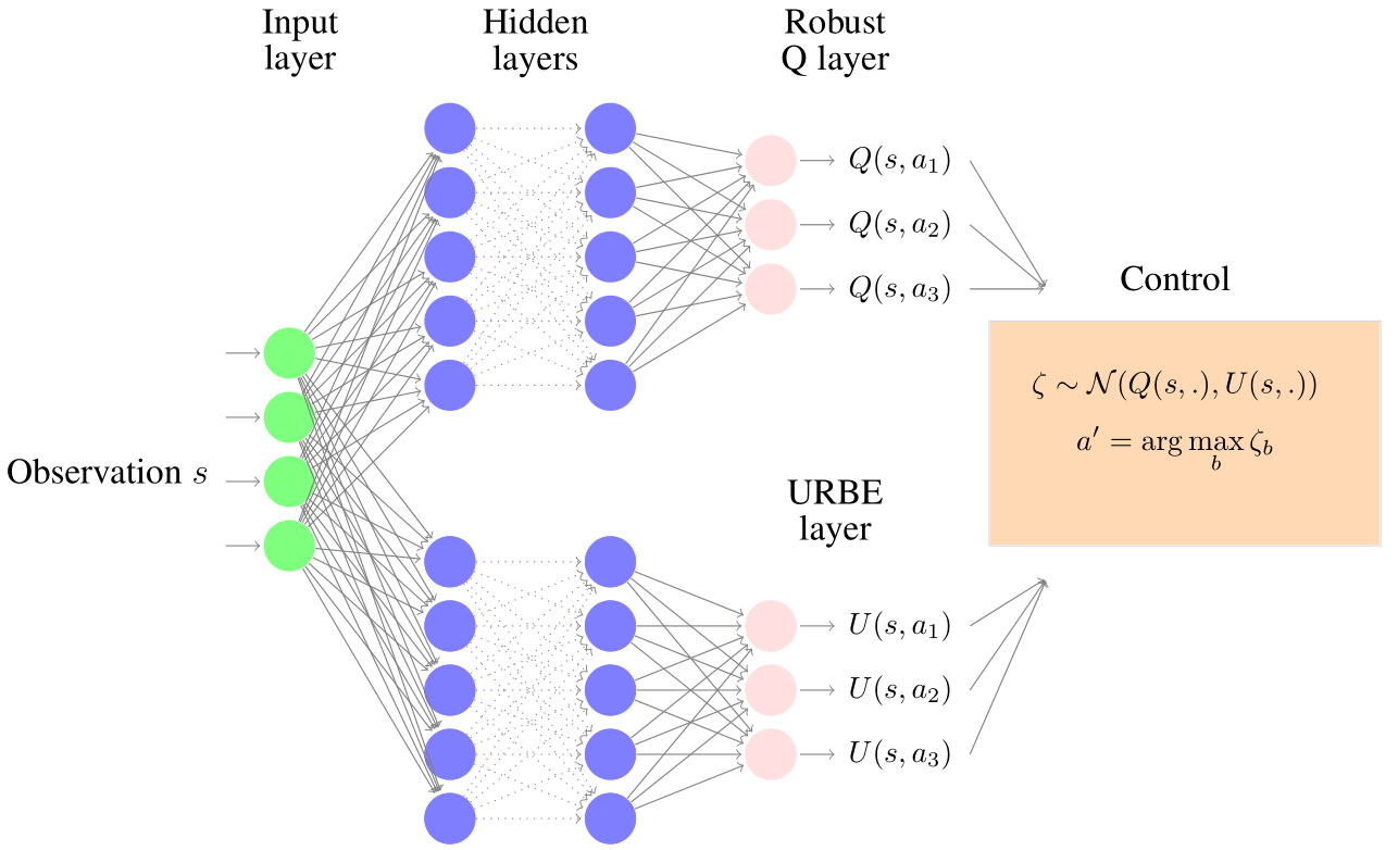
DQN-URBE consists of a neural network architecture that has two output heads, as shown in Figure 1. The first head attempts to learn the optimal robust Q-function of a fixed uncertainty set via the robust-DQN subroutine described in [Di-Castro Shashua and Mannor, 2017]. It is similar to regular DQN except that it utilizes the robust TD-error as a loss criterion. The other head attempts to estimate the robust uncertainty for the robust Q-function, as mentioned in Section 4.3. The robust local uncertainty is estimated using the function approximation method described in Section 5. This defines the loss function to minimize for learning the robust local uncertainty parameters. We added stop-gradients to prevent the posterior variance from affecting the robust Q-network parameters and vice-versa. At each step, the agent acts greedily with respect to the robust Q-function plus the robust local uncertainty to encourage exploration.

Figure 2: (a) Simple MDP illustration, with initial and terminating state $s_{0}$. (b) Comparison of the accumulated rewards on the simple MDP. The vertical lines mark changing dynamics. (c) Mar’s Rover domain. Starting states are randomly chosen from the red zone. The goal state is in orange.

7 EXPERIMENTS

In this section, we test the performance of our URBE-based approach on three different domains: a toy MDP, a Mar’s Rover domain and Cartpole. We first execute URBE on a toy MDP and analyze its performance under changing dynamics. We then propose DQN-URBE, a deep RL algorithm that scales our URBE approach to higher dimensional domains. We run and analyze the performance of DQN-URBE on a Mar’s rover domain and Cartpole. In each case, we compare the robust DQN-URBE policy to three baselines: (1) a vanilla DQN; (2) an overly conservative, robust DQN agent and (3) a DQN that uses UBE for exploration [O’Donoghue et al., 2018]. Neural network structures and hyperparameters can be found in the Appendix.

7.1 SIMPLE MDP

We consider a variant of the 7-state MDP introduced in [Lim et al., 2016b], which is illustrated in Figure 2. The agent starts from state $s_{0}$ and chooses one of $4$ actions. Action $a_{1}$ leads to a purely deterministic outcome, whereas $a_{2},a_{3}$ and $a_{4}$ may be subject to adversarial transitions and lead the agent to either state $s_{3}$ or $s_{6}$. The agent is brought back to the terminating state $s_{0}$ once it reached $s_{1}$, $s_{3}$ or $s_{6}$. These latter states are the only ones with non-zero rewards, although in practice, we set $R(s_{6})=0$, $R(s_{1})=0.14$ and $R(s_{3})=1$.

This MDP captures the main characteristics of a grid-world domain in which the agent must reach a gold state under adversarial transitions. At any episode, an adversary can choose any transition probability $p(s_{3})$ for the agent to reach the gold state $s_{3}$ from $s_{2},s_{4}$ or $s_{5}$. If it behaves nicely and $p(s_{3})=1$, the agent can achieve maximal reward. However, if $p(s_{3})=0$, the agent is brought to the ”bad state” $s_{6}$ in case it did not choose action $a_{1}$, and thus gets minimal reward. For a fixed uncertainty that accounts for all adversarial transitions, a minimax-optimal policy corresponds to constantly taking action $a_{1}$.

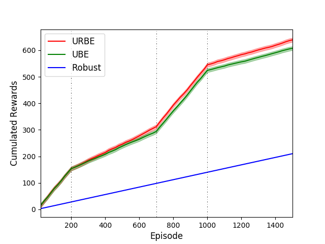
Figure 2 shows the accumulated rewards over running time for the described MDP, and each vertical line marks a change in the adversarial probability $p(s_{3})$. We successively set such probability to $0.001,0.8,0.1$ and $0.9$. Cumulative rewards have been averaged over $10$ runs for UBE and URBE, whereas the performance of the robust policy is deterministic. As we can see in the figure, the robust agent is overly conservative although its reward is stable under adversarial transitions. Also, since the UBE-based agent does not account for adversarial transitions, it performs worse than URBE.

7.2 MAR’S ROVER

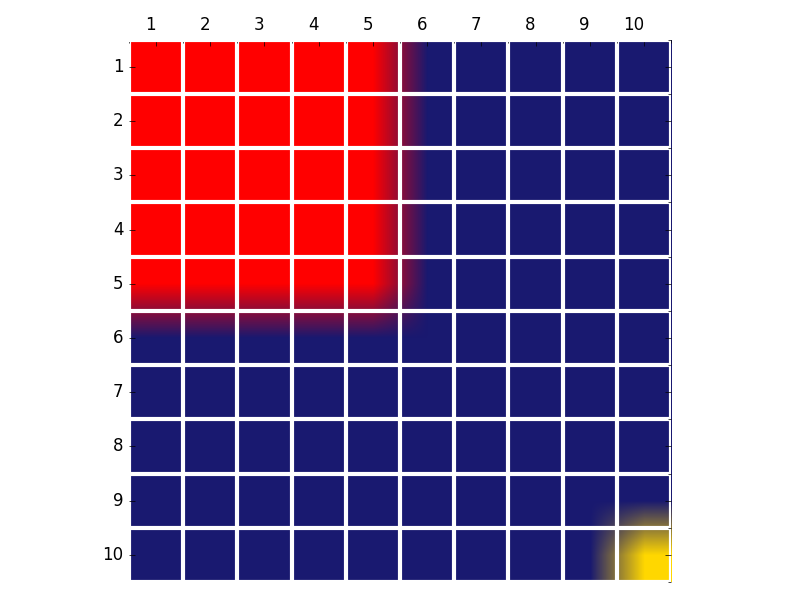
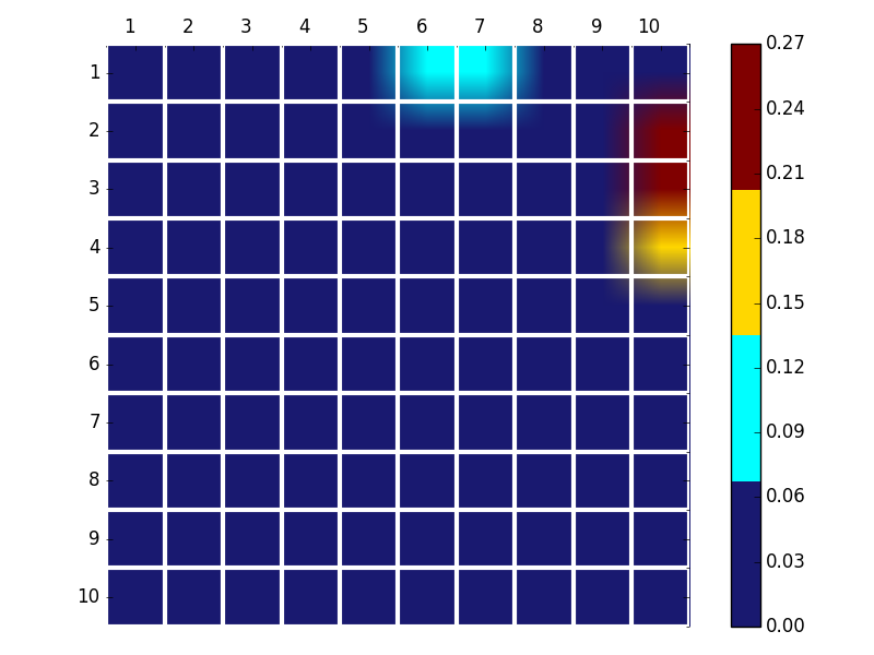
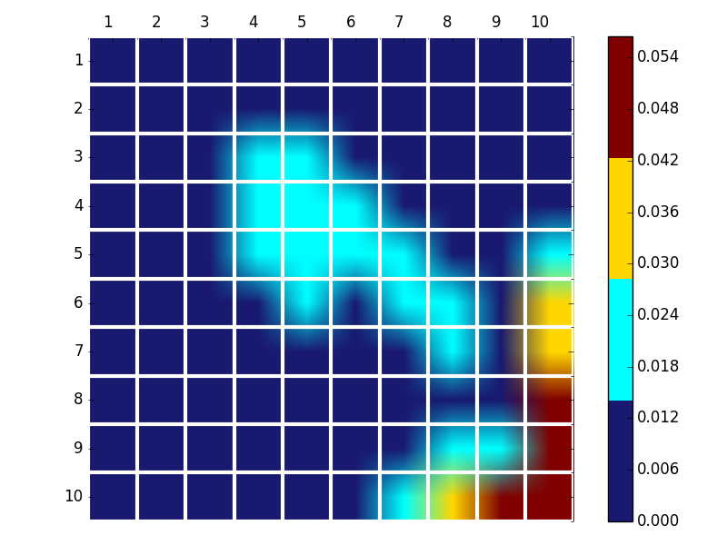
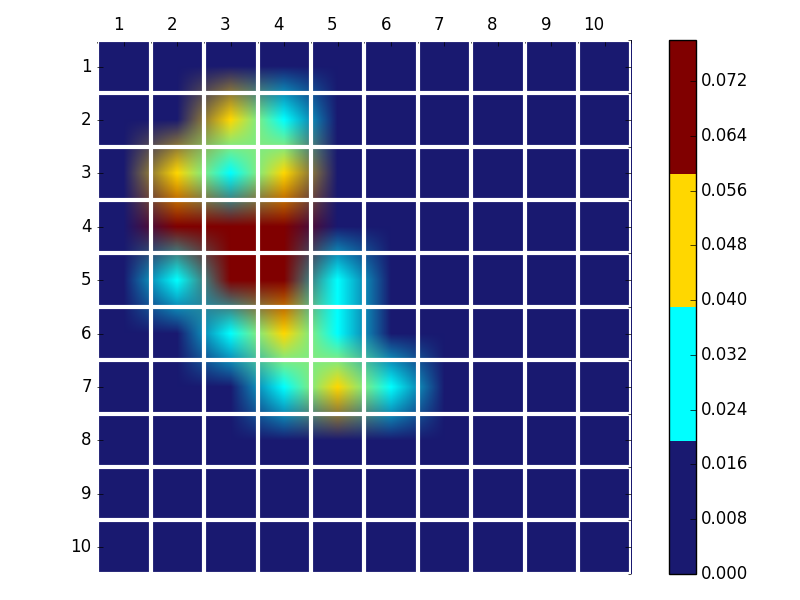
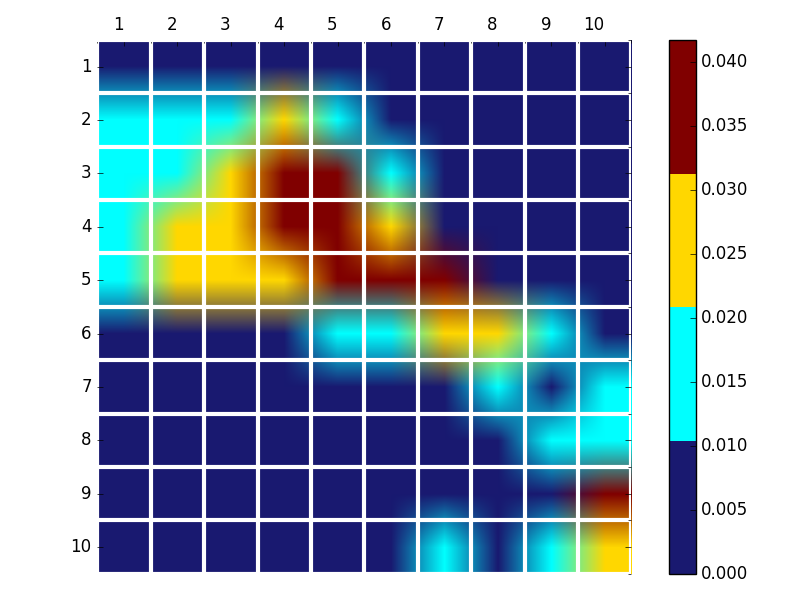
We extend the size of the previous MDP and consider a $10\times 10$ grid-world domain inspired by [Chow et al., 2015; Tessler et al., 2019]. A rover starts at a random state from the top left of the grid (red zone in Figure 2) and is required to travel to the goal located in the bottom right corner (orange square in Figure 2) in less than $200$ steps so as to get a high reward $R_{\text{success}}$. The transition is stochastic. On each step, if it chooses to move towards the goal, the agent may be brought back to a final state and get a negative reward $R_{\text{fail}}$ with probability $p$. Otherwise, it moves into the chosen direction and receives a small negative reward $R_{\text{step}}$.

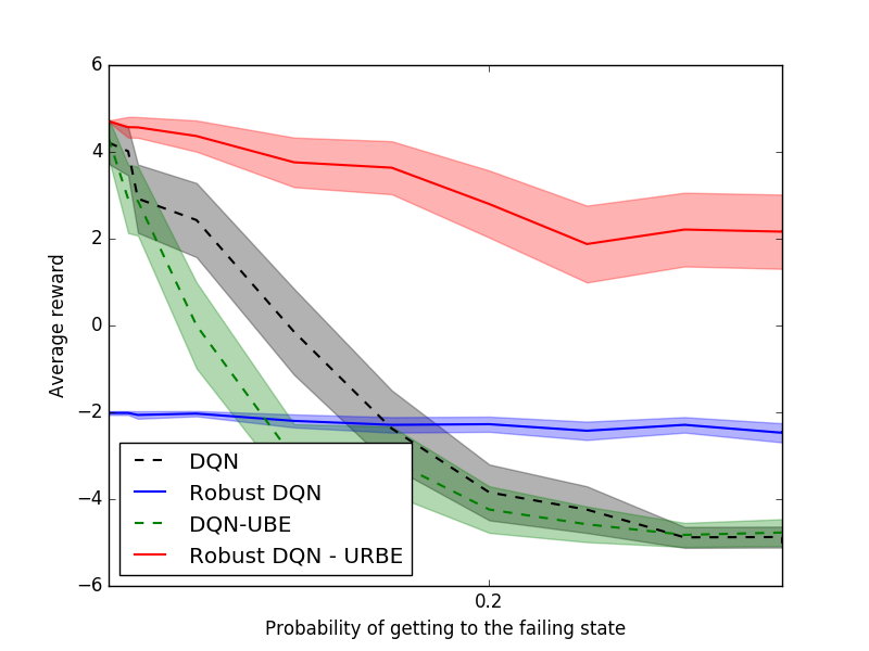
We trained vanilla DQN, robust DQN, DQN-UBE and DQN-URBE on a nominal probability of failure $p=0.005$. Uncertainty sets were generated by sampling $15$ probabilities $p$ in $(0,1)$. Figure 3 shows the testing performance of each strategy over different probabilities. We see that the robust agent is unable to reach the goal state, even on the nominal model. However, it is never brought back to the failing state but rather avoids moving towards the goal state, which explains its stable performance. Similarly to vanilla DQN, the UBE agent performs well on the nominal but is most sensitive to changing dynamics. Its reward gets even worse than robust DQN above $p=0.2$, since it tries to move towards the goal but is barred by adversarial transitions. During testing, DQN-URBE reaches high reward on the nominal model and shows less sensitivity to increasing probabilities. It is therefore less conservative than robust DQN but stays robust to model misspecification.

We further investigated the trajectories of three agents across the grid, under appropriate dynamics. A number of $100$ testing episodes were run. Figure 4 represents heatmaps of states that were attained, with their proportion of visits. These are visualized in four colors, ranging from the lowest to the highest proportion: dark blue, cyan, yellow and brown. Figures 4 and 4 correspond to testing episodes on the nominal model $p=0.005$ for robust DQN and URBE, respectively. The robust agent never reaches the goal, while URBE shows high proportion of visitation on the winning state. In Figures 4 and 4, a higher probability of failure ($p=0.2$) has been used to test the robustness of DQN-UBE against DQN-URBE. The URBE agent clearly shows more robustness than UBE, as it reaches the goal state under this mispecified model.

Figure 3: Testing rewards on Mar’s Rover.

Figure 4: Mar’s Rover heatmaps of state visitations during $100$ testing episodes. (a) Robust DQN on $p=0.005$. (b) DQN-URBE on $p=0.005$. (c) DQN-UBE on $p=0.2$. (d) DQN-URBE on $p=0.2$. Robust DQN is too conservative compared to URBE, while UBE is less robust than URBE.

7.3 CARTPOLE

In Cartpole, the agent’s goal is to balance a pole atop a cart in a vertical position. The system corresponds to a continuous MDP where each state is a 4-tuple $\langle x,\dot{x},\theta,\dot{\theta}\rangle$ representing the cart position, the cart speed, the pole angle with respect to the vertical and its angular speed respectively. The agent can make one of two actions: apply a constant force either to the right or to the left of the pole. It gets a reward of $1$ if the pole has not fallen down and if it stayed in the boundary sides of the screen. If it terminates, the agent receives a reward of $0$. Each episode lasts for $200$ steps.

Figure 5: Testing rewards on Cartpole.

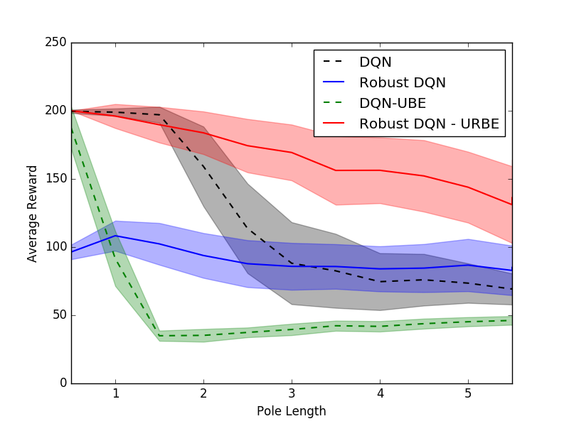
All agents have been trained on a nominal pole length of $0.75$. Uncertainty sets were generated by sampling $15$ lengths from a normal distribution centered at the nominal. The agents were then tested over $200$ episodes on different pole lengths. Figure 5 shows their average reward during testing. Robust DQN is overly conservative on the nominal length although it stays robust to model misspecification, compared to DQN-UBE which is most sensitive to changing pole lengths. On the other hand, DQN-URBE shows the best trade-off between less conservativeness on the nominal and robustness to higher lengths. This leads it to perform best on the nominal length and on higher ones as well.

Figure 6: (a-b) Cartpole on the nominal model. These figures show the states $\langle x,\theta\rangle$ attained and the two colors correspond to the action applied on these states. (a) DQN-URBE; (b) Robust DQN. (c) Training score of DQN-URBE and robust DQN. Vertical lines mark changes of the pole length. DQN-URBE explores more than robust DQN while it stays robust to changing dynamics.

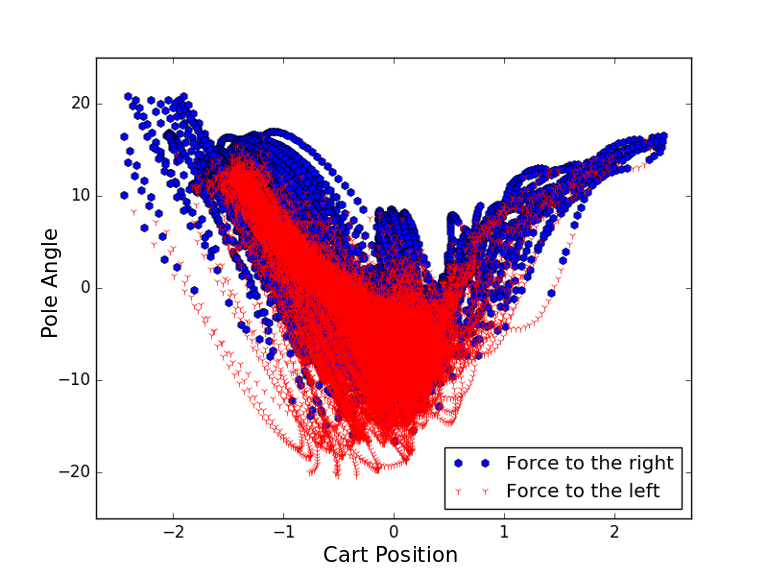
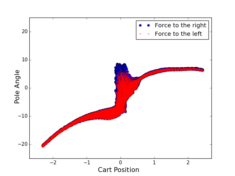
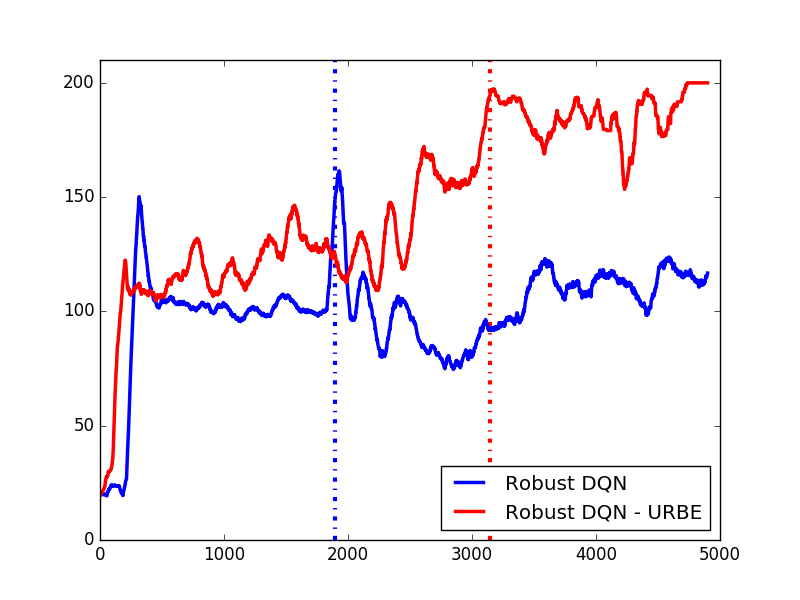
In order to further test the exploration capacity of the robust agents, we also compared the projected states $\langle x,\theta\rangle$ attained on the nominal model during $200$ testing episodes. Figures 6 and 6 show that the span of visited states for the robust agent is quite limited compared to URBE, which may explain its overly conservative behavior. We also compared the sensitivity of robust DQN with that of DQN-URBE to changing dynamics during training. In practice, we waited for both agents to converge before changing the pole length from $0.75$ to $1.25$. We also augmented the number of training episodes from $4000$ to $5000$. Figure 6 shows a smoothed version of the training curve. Changes in dynamics are marked by vertical lines, and each color is that of the corresponding agent. As can be seen in the figure, although URBE converges more slowly, it recovers much faster than robust DQN which does not recover at all to its optimal reward. Moreover, URBE is able to reach maximal reward.

Table 1: Comparison of previous approaches with URBE

Reference	Mitigates RMDPs Conservativeness	Online Learning of an Uncertainty Set	Scalability
URBE (this paper)	$\surd$	$\surd$	$\surd$
[Goyal and Grand-Clement, 2019]	$\surd$	$\times$	$\times$
[Tirinzoni et al., 2018]	$\surd$	$\times$	$\surd$
[Petrik and Russell, 2019]	$\surd$	$\times$	$\times$
[Derman et al., 2018]	$\surd$	$\times$	$\surd$
[Lim et al., 2016b]	$\surd$	$\surd$	$\times$
[Mannor et al., 2012, 2016]	$\surd$	$\times$	$\times$
[Xu and Mannor, 2012; Yu and Xu, 2016]	$\surd$	$\times$	$\times$

8 RELATED WORK

Several methods have been proposed to mitigate conservativeness in robust RL. These are indicated in Table 1. These works can be collectively grouped into three distinct approaches for mitigating the conservativeness of RMDPs. The first one focuses on circumventing rectangular uncertainty sets. This includes works [Mannor et al., 2012, 2016] that consider coupled uncertainties which still lead to tractable solutions for the robust RL problem. Similarly, in [Tirinzoni et al., 2018], the authors proposed the construction of non-rectangular uncertainty sets that take advantage of transfer knowledge between states. More recently, the work [Goyal and Grand-Clement, 2019] introduced an uncertainty set structured as an ambiguous linear function of a factor matrix and showed that the underlying minimax policy is computationally tractable.

A second approach for overcoming conservativeness of robust RL is to consider a distribution over the uncertainty set rather than its worst-case model. In [Xu and Mannor, 2012; Yu and Xu, 2016], structural information on parameter distribution is assumed. It is used for deriving an optimal policy under the worst parameter distribution using distributionally robust optimization. In [Derman et al., 2018], the authors showed that if we fix such a distribution, the corresponding optimal policy interpolates between being aggressive and robust. Nonetheless, as indicated in the second column of Table 1, all of these approaches address the problem of planning in robust MDPs or its variants without learning the uncertainty set in an online manner. Therefore, they cannot adapt it to changing dynamics.

Conversely, a third approach involves learning adversarial transitions and/or rewards. The work [Lim et al., 2016b] considered the problem of learning the uncertainty set in a frequentist setting and used OFU methods for detecting adversarial states and updating the uncertainty set accordingly. Although the resulting algorithm is online and provably efficient, it is not scalable to large domains and its efficiency strongly relies on the statistical analysis. Using a Bayesian setting in [Petrik and Russell, 2019], the authors addressed an algorithm that constructs Bayesian uncertainty sets in a safe manner. However, besides learning an uncertainty set offline with a fixed batch of data, their method is not scalable because of its computational cost. In contrast, our proposed approach aims to adapt the level of robustness iteratively and online from a dynamic stream of data.

9 CONCLUSION

We presented a Bayesian approach to learning less conservative solutions when solving Robust MDPs. This is achieved using the Uncertainty Robust Bellman Equation (URBE), our adaptation of the UBE equation, which encourages safe exploration and implicitly modifies the uncertainty set online using new observations. We scale this approach to higher dimensional domains using the DQN-URBE algorithm and show the ability of the agent to learn less conservative solutions in a toy MDP, a Mar’s rover domain and Open AI gym’s Cartpole domain. Finally, we show the ability of the agent to adapt to changing dynamics significantly faster than a robust DQN agent during training. Our approach shed light on the advantages of adding a variance bonus to robust Q-learning for encouraging safe exploration in lowering the conservativeness of robust strategies. Further work should analyze the asymptotic behavior of our URBE-based method as well as the impact of the size of the posterior uncertainty set on the posterior variance of robust Q-values.

Acknowledgements

The authors would like to thank Chen Tessler for his help and useful comments on this work. E. Derman would like to acknowledge the support of the Israel Science Foundation grant.

A Bayesian Approach to Robust Reinforcement Learning - Appendix

Appendix A Theoretical Proofs

Recall the assumptions made in the paper:

Assumption A.1.

For any episode, the graph resulting from a worst-case transition model is directed and acyclic.

Assumption A.2.

For all $(s,a)\in\mathcal{S}\times\mathcal{A}$, the rewards are bounded: $-R_{\max}\leq r_{sa}\leq R_{\max}$. This implies that the robust Q-value is bounded as well: $\mid Q_{sa}^{h}\mid\leq HR_{\max}=:Q_{\max}$.

Recall also the worst-case transition from a posterior uncertainty set:

$$\begin{split}\widehat{Q}_{sa}^{h}&=r_{sa}^{h}+\gamma\inf_{p\in\widehat{\mathcal{P}}_{sa}^{h}}\sum_{s^{\prime},a^{\prime}}\pi_{s^{\prime}a^{\prime}}^{h}p_{sas^{\prime}}\widehat{Q}_{s^{\prime}a^{\prime}}^{h+1}\enspace,\end{split}$$

with $\widehat{Q}_{sa}^{H+1}=0$ and

$$\begin{split}\widehat{p}_{sa}^{h}&\in\arg\min_{p\in\widehat{\mathcal{P}}_{sa}^{h}}\sum_{s^{\prime},a^{\prime}}\pi_{s^{\prime}a^{\prime}}^{h}p_{sas^{\prime}}\widehat{Q}_{s^{\prime}a^{\prime}}^{h+1}\end{split}$$ (4)

is a worst-case transition at step $h$.

A.1 Proof of Lemma 4.1

Lemma A.1.

Under Assumptions A.1 and A.2, for any worst-case transition $\widehat{p}$ as defined in equation (4), the conditional variance of the robust Q-values under the posterior distribution satisfies the robust Bellman inequality:

$$\mathbf{var}_{t}\widehat{Q}_{sa}^{h}\leq\nu_{sa}^{h}+\gamma^{2}\sum_{s^{\prime},a^{\prime}}\pi_{s^{\prime}a^{\prime}}^{h}\mathbb{E}_{t}\left(\widehat{p}_{sas^{\prime}}^{h}\right)\mathbf{var}_{t}\widehat{Q}_{s^{\prime}a^{\prime}}^{h+1},$$

with $\mathbf{var}_{t}\widehat{Q}^{H+1}=0$ and $\nu_{sa}^{h}:=Q^{2}_{\max}\sum_{s^{\prime}\in\mathcal{S}}\frac{\mathbf{var}_{t}\widehat{p}_{sas^{\prime}}^{h}}{\mathbb{E}_{t}\widehat{p}_{sas^{\prime}}^{h}}$.

Proof.

The proof for the robust setup follows the same line as in [O’Donoghue et al., 2018] and is given here for completeness.

First rewrite the conditional variance:

$$\begin{split}&\text{var}_{t}(\widehat{Q}_{sa}^{h}):=\mathbb{E}_{t}\left(\widehat{Q}_{sa}^{h}-\mathbb{E}_{t}\widehat{Q}_{sa}^{h}\right)^{2}\\ &=\mathbb{E}_{t}\left(\gamma\inf_{p\in\widehat{\mathcal{P}}_{sa}^{h}}\sum_{s^{\prime},a^{\prime}}\pi_{s^{\prime}a^{\prime}}^{h}p^{h}_{sas^{\prime}}\widehat{Q}_{s^{\prime}a^{\prime}}^{h+1}-\gamma\mathbb{E}_{t}\inf_{p\in\widehat{\mathcal{P}}_{sa}^{h}}\sum_{s^{\prime},a^{\prime}}\pi_{s^{\prime}a^{\prime}}^{h}p^{h}_{sas^{\prime}}\widehat{Q}_{s^{\prime}a^{\prime}}^{h+1}\right)^{2}\\ &=\gamma^{2}\mathbb{E}_{t}\left(\sum_{s^{\prime},a^{\prime}}\pi_{s^{\prime}a^{\prime}}^{h}\widehat{p}^{h}_{sas^{\prime}}\widehat{Q}_{s^{\prime}a^{\prime}}^{h+1}-\mathbb{E}_{t}\sum_{s^{\prime},a^{\prime}}\pi_{s^{\prime}a^{\prime}}^{h}\widehat{p}^{h}_{sas^{\prime}}\widehat{Q}_{s^{\prime}a^{\prime}}^{h+1}\right)^{2}\\ &=\gamma^{2}\mathbb{E}_{t}\left(\sum_{s^{\prime},a^{\prime}}\pi_{s^{\prime}a^{\prime}}^{h}\left(\widehat{p}^{h}_{sas^{\prime}}\widehat{Q}_{s^{\prime}a^{\prime}}^{h+1}-\mathbb{E}_{t}\widehat{p}^{h}_{sas^{\prime}}\widehat{Q}_{s^{\prime}a^{\prime}}^{h+1}\right)\right)^{2},\end{split}$$

where we used the following definitions:

$$\begin{split}&\widehat{Q}_{sa}^{h}=r_{sa}^{h}+\gamma\inf_{p\in\widehat{\mathcal{P}}_{sa}^{h}}\sum_{s^{\prime},a^{\prime}}\pi_{s^{\prime}a^{\prime}}^{h}p_{sas^{\prime}}^{h}\widehat{Q}_{s^{\prime}a^{\prime}}^{h+1}\\ &\widehat{p}_{sa}^{h}\in\arg\inf_{p\in\widehat{\mathcal{P}}_{sa}^{h}}\sum_{s^{\prime},a^{\prime}}\pi_{s^{\prime}a^{\prime}}^{h}p_{sas^{\prime}}^{h}\widehat{Q}_{s^{\prime}a^{\prime}}^{h+1}.\end{split}$$

Assume that $\mathbb{E}_{t}\widehat{p}_{sas^{\prime}}>0$ for all $h,s,a,s^{\prime}$ belonging to the adequate sets. Since any worst-case transition satisfies $\sum_{s^{\prime}}\widehat{p}^{h}_{sas^{\prime}}=1$, we have $\sum_{s^{\prime},a^{\prime}}\pi_{s^{\prime}a^{\prime}}\mathbb{E}_{t}\widehat{p}^{h}_{sas^{\prime}}=1$ and $\pi_{s^{\prime}a^{\prime}}\mathbb{E}_{t}\widehat{p}^{h}_{sas^{\prime}}$ defines a probability distribution over states and actions. Thus,

$$\begin{split}\quad\mathbb{E}_{t}\left(\sum_{s^{\prime},a^{\prime}}\pi_{s^{\prime}a^{\prime}}^{h}\left(\widehat{p}^{h}_{sas^{\prime}}\widehat{Q}_{s^{\prime}a^{\prime}}^{h+1}-\mathbb{E}_{t}\widehat{p}^{h}_{sas^{\prime}}\widehat{Q}_{s^{\prime}a^{\prime}}^{h+1}\right)\right)^{2}&=\mathbb{E}_{t}\left(\sum_{s^{\prime},a^{\prime}}\pi_{s^{\prime}a^{\prime}}^{h}\frac{\mathbb{E}_{t}\widehat{p}^{h}_{sas^{\prime}}}{\mathbb{E}_{t}\widehat{p}^{h}_{sas^{\prime}}}(\widehat{p}^{h}_{sas^{\prime}}\widehat{Q}_{s^{\prime}a^{\prime}}^{h+1}-\mathbb{E}_{t}\sum_{s^{\prime},a^{\prime}}\widehat{p}^{h}_{sas^{\prime}}\widehat{Q}_{s^{\prime}a^{\prime}}^{h+1})\right)^{2}\\ &\leq\sum_{s^{\prime},a^{\prime}}\pi_{s^{\prime}a^{\prime}}^{h}\frac{\mathbb{E}_{t}\widehat{p}^{h}_{sas^{\prime}}}{\left(\mathbb{E}_{t}\widehat{p}^{h}_{sas^{\prime}}\right)^{2}}\mathbb{E}_{t}\left(\widehat{p}^{h}_{sas^{\prime}}\widehat{Q}_{s^{\prime}a^{\prime}}^{h+1}-\mathbb{E}_{t}\sum_{s^{\prime},a^{\prime}}\widehat{p}^{h}_{sas^{\prime}}\widehat{Q}_{s^{\prime}a^{\prime}}^{h+1}\right)^{2},\end{split}$$

by applying Jensen’s inequality to the convex function $x\mapsto x^{2}$. Therefore,

$$\begin{split}\text{var}_{t}(\widehat{Q}_{sa}^{h})\leq\sum_{s^{\prime},a^{\prime}}\pi_{s^{\prime}a^{\prime}}^{h}\frac{\mathbb{E}_{t}\widehat{p}^{h}_{sas^{\prime}}}{\left(\mathbb{E}_{t}\widehat{p}^{h}_{sas^{\prime}}\right)^{2}}\mathbb{E}_{t}\left(\widehat{p}^{h}_{sas^{\prime}}\widehat{Q}_{s^{\prime}a^{\prime}}^{h+1}-\mathbb{E}_{t}\widehat{p}^{h}_{sas^{\prime}}\widehat{Q}_{s^{\prime}a^{\prime}}^{h+1}\right)^{2}\end{split}$$

Rewriting $\widehat{Q}_{s^{\prime}a^{\prime}}^{h+1}=r_{s^{\prime}a^{\prime}}^{h+1}+\gamma\inf_{p\in\widehat{\mathcal{P}}_{s^{\prime}a^{\prime}}^{h+1}}\sum_{s^{\prime\prime},a^{\prime\prime}}\pi_{s^{\prime\prime}a^{\prime\prime}}^{h+1}p_{s^{\prime\prime}s^{\prime}a^{\prime}}^{h+1}\widehat{Q}_{s^{\prime\prime}a^{\prime\prime}}^{h+2}$ and $\widehat{p}_{sa}^{h}=\arg\inf_{p\in\widehat{\mathcal{P}}_{sa}^{h}}\sum_{s^{\prime},a^{\prime}}\pi_{s^{\prime}a^{\prime}}^{h}p_{sas^{\prime}}^{h}\widehat{Q}_{s^{\prime}a^{\prime}}^{h+1}$ enables us to claim that under Assumption A.1, $\widehat{p}_{sa}^{h}$ is independent of $\widehat{Q}_{sa}^{h+1}$ conditionally on $\mathcal{F}_{t}$, because $\widehat{Q}_{s^{\prime}a^{\prime}}^{h+1}$ depends on downstream uncertainty sets. Note that this claim relies on the rectangular structure of the uncertainty set. Thus,

$$\begin{split}\mathbb{E}_{t}\left(\widehat{p}^{h}_{sas^{\prime}}\widehat{Q}_{s^{\prime}a^{\prime}}^{h+1}-\mathbb{E}_{t}\widehat{p}^{h}_{sas^{\prime}}\widehat{Q}_{s^{\prime}a^{\prime}}^{h+1}\right)^{2}&=\mathbb{E}_{t}\left((\widehat{p}^{h}_{sas^{\prime}}-\mathbb{E}_{t}\widehat{p}^{h}_{sas^{\prime}})\widehat{Q}_{s^{\prime}a^{\prime}}^{h+1}+\mathbb{E}_{t}\widehat{p}^{h}_{sas^{\prime}}(\widehat{Q}_{s^{\prime}a^{\prime}}^{h+1}-\mathbb{E}_{t}\widehat{Q}_{s^{\prime}a^{\prime}}^{h+1})\right)^{2}\\ &=\mathbb{E}_{t}\left((\widehat{p}^{h}_{sas^{\prime}}-\mathbb{E}_{t}\widehat{p}^{h}_{sas^{\prime}})\widehat{Q}_{s^{\prime}a^{\prime}}^{h+1}\right)^{2}+\mathbb{E}_{t}\left(\widehat{p}^{h}_{sas^{\prime}}(\widehat{Q}_{s^{\prime}a^{\prime}}^{h+1}-\mathbb{E}_{t}\widehat{Q}_{s^{\prime}a^{\prime}}^{h+1})\right)^{2}.\end{split}$$

We use the conditional independence property again and Assumption A.2 in order to deduce the following:

$$\begin{split}\mathbb{E}_{t}\left((\widehat{p}^{h}_{sas^{\prime}}-\mathbb{E}_{t}\widehat{p}^{h}_{sas^{\prime}})\widehat{Q}_{s^{\prime}a^{\prime}}^{h+1}\right)^{2}&=\mathbb{E}_{t}(\widehat{p}^{h}_{sas^{\prime}}-\mathbb{E}_{t}\widehat{p}^{h}_{sas^{\prime}})^{2}\mathbb{E}_{t}(\widehat{Q}_{s^{\prime}a^{\prime}}^{h+1})^{2}\leq Q_{\max}^{2}\mathbf{var}_{t}\widehat{p}^{h}_{sas^{\prime}},\\ \text{and }\mathbb{E}_{t}\left(\widehat{p}^{h}_{sas^{\prime}}(\widehat{Q}_{s^{\prime}a^{\prime}}^{h+1}-\mathbb{E}_{t}\widehat{Q}_{s^{\prime}a^{\prime}}^{h+1})\right)^{2}&=\mathbb{E}_{t}(\widehat{p}^{h}_{sas^{\prime}})^{2}\mathbb{E}_{t}(\widehat{Q}_{s^{\prime}a^{\prime}}^{h+1}-\mathbb{E}_{t}\widehat{Q}_{s^{\prime}a^{\prime}}^{h+1})^{2}=\mathbb{E}_{t}(\widehat{p}^{h}_{sas^{\prime}})^{2}\mathbf{var}_{t}\widehat{Q}_{s^{\prime}a^{\prime}}^{h+1}.\end{split}$$

Finally,

$$\begin{split}\text{var}_{t}(\widehat{Q}_{sa}^{h})&\leq\gamma^{2}\sum_{s^{\prime},a^{\prime}}\pi_{s^{\prime}a^{\prime}}^{h}\frac{\mathbb{E}_{t}\widehat{p}^{h}_{sas^{\prime}}}{\left(\mathbb{E}_{t}\widehat{p}^{h}_{sas^{\prime}}\right)^{2}}(Q_{\max}^{2}\mathbf{var}_{t}\widehat{p}^{h}_{sas^{\prime}}+\mathbb{E}_{t}(\widehat{p}^{h}_{sas^{\prime}})^{2}\mathbf{var}_{t}\widehat{Q}_{s^{\prime}a^{\prime}}^{h+1})\\ &\leq\gamma^{2}\sum_{s^{\prime},a^{\prime}}\pi_{s^{\prime}a^{\prime}}^{h}\frac{\mathbb{E}_{t}\widehat{p}^{h}_{sas^{\prime}}}{\left(\mathbb{E}_{t}\widehat{p}^{h}_{sas^{\prime}}\right)^{2}}Q_{\max}^{2}\mathbf{var}_{t}\widehat{p}^{h}_{sas^{\prime}}+\gamma^{2}\sum_{s^{\prime},a^{\prime}}\pi_{s^{\prime}a^{\prime}}^{h}\mathbb{E}_{t}\widehat{p}^{h}_{sas^{\prime}}\mathbf{var}_{t}\widehat{Q}_{s^{\prime}a^{\prime}}^{h+1}\\ &\leq Q_{\max}^{2}\sum_{s^{\prime}}\frac{\mathbf{var}_{t}\widehat{p}^{h}_{sas^{\prime}}}{\mathbb{E}_{t}\widehat{p}^{h}_{sas^{\prime}}}+\gamma^{2}\sum_{s^{\prime},a^{\prime}}\pi_{s^{\prime}a^{\prime}}^{h}\mathbb{E}_{t}\widehat{p}^{h}_{sas^{\prime}}\mathbf{var}_{t}\widehat{Q}_{s^{\prime}a^{\prime}}^{h+1}\\ &\leq\nu_{sa}^{h}+\gamma^{2}\sum_{s^{\prime},a^{\prime}}\pi_{s^{\prime}a^{\prime}}^{h}\mathbb{E}_{t}\widehat{p}^{h}_{sas^{\prime}}\mathbf{var}_{t}\widehat{Q}_{s^{\prime}a^{\prime}}^{h+1},\end{split}$$

where $\nu_{sa}^{h}$ is given by $\nu_{sa}^{h}:=Q_{\max}^{2}\sum_{s^{\prime}}\frac{\mathbf{var}_{t}\widehat{p}^{h}_{sas^{\prime}}}{\mathbb{E}_{t}\widehat{p}^{h}_{sas^{\prime}}}$. ∎

A.2 Proof of Theorem 4.1

Theorem A.1 (Solution of URBE).

For any worst-case transition $\widehat{p}$ as defined in equation (4) and any policy $\pi$, under Assumptions A.1 and A.2, there exists a unique mapping $w$ that satisfies the uncertainty robust Bellman equation:

$$w_{sa}^{h}=\nu_{sa}^{h}+\gamma^{2}\sum_{s^{\prime}\in\mathcal{S},a^{\prime}\in\mathcal{A}}\pi_{s^{\prime}a^{\prime}}^{h}\mathbb{E}_{t}(\widehat{p}_{sas^{\prime}}^{h})w_{s^{\prime}a^{\prime}}^{h+1},$$ (5)

for all $(s,a)\in\mathcal{S}\times\mathcal{A}$ and $h=1,\cdots,H$ where $w^{H+1}=0$. Furthermore, $w\geq\mathbf{var}_{t}\widehat{Q}$.

Proof.

Denote by $\mathcal{W}^{h}$ the robust Bellman operator underlying equation (5) and rewrite is as $\mathcal{W}^{h}w^{h+1}=w^{h}$. We can easily see that the robust Bellman operator is non-decreasing. Also, it has a unique solution, as stated in the following lemma, which is the policy evaluation version of the Min-Max Problem addressed in [Bertsekas, 2000] (Exercise 1.5).

Lemma A.2.

For every $(s,a)\in\mathcal{S}\times\mathcal{A}$, for all step $h=1,\cdots,H$, $w_{sa}^{h}$ is given by the subsequent steps of the following algorithm which proceeds backwards from $H+1$ to $h$:

$$\left\{\begin{array}[]{ll}w_{sa}^{H+1}=0\text{ for all }(s,a)\in\mathcal{S}\times\mathcal{A}\\ w_{sa}^{h}=\nu_{sa}^{h}+\gamma^{2}\sum_{s^{\prime}\in\mathcal{S},a^{\prime}\in\mathcal{A}}\pi_{s^{\prime}a^{\prime}}^{h}\mathbb{E}_{t}(\widehat{p}_{sas^{\prime}}^{h})w_{s^{\prime}a^{\prime}}^{h+1}\end{array}\right.$$

Therefore, there exists a unique solution to $\mathcal{W}^{h}w^{h+1}=w^{h},h=1,\cdots,H$.

The lower-bound then follows from induction reasoning. At step $H$, we have $\mathbf{var}_{t}\widehat{Q}^{H+1}=0=w^{H+1}$. Assume that for some $h\leq H$ we have $w^{h+1}\geq\mathbf{var}_{t}\widehat{Q}^{h+1}$. Then, by assumption and using Lemma A.1, we get:

$$\begin{split}\mathbf{var}_{t}\widehat{Q}^{h}\leq\mathcal{W}^{h}\mathbf{var}_{t}\widehat{Q}^{h+1}&\leq\mathcal{W}^{h}w^{h+1}=w^{h}.\end{split}$$

The induction property is hereditary, which concludes the proof of the theorem. ∎

Appendix B DQN-URBE Experiments

Table 2: System’s dynamics

	MARSROVER	CARTPOLE
Nominal model	$p=0.005$	Length = $0.75$, Mass = $1$
Size of uncertainty set	15 samples	15 samples

Table 3: Networks

DQN-URBE NETWORKS	MARSROVER	CARTPOLE
Q-network	ReLu(2 hidden layers of size 10)	ReLu(3 hidden layers of size 128)
U(R)BE-network	ReLu(1 hidden layer of size 15),	ReLu(1 hidden layer of size 100),
	linear activation function for the output	linear activation function for the output

Table 4: Hyper-parameters

DQN-URBE HYPERPARAMETERS	MARSROVER	CARTPOLE
Discount factor $\gamma$	$0.9$	$0.9$
Q-learning rate	1e-4	1e-4
U(R)BE network learning rate	1e-4	1e-4
Initial variance coefficient $\mu$	1e-2	1e-2
Posterior parameter $\beta$	$0.5$	$0.5$
Mini-batch size	$100$	$256$
Final epsilon	1e-3	1e-5
Target update interval	$10$	$10$
Max number of episodes for training $M_{train}$	$3000$	$4000$
Number of episodes for testing $M_{test}$	$200$	$200$

References

- Berger [2013] James O. Berger. Statistical Decision Theory and Bayesian Analysis. Springer Science and Business Media, 2013.
- Bertsekas [2000] Dimitri P. Bertsekas. Dynamic Programming and Optimal Control, volume 1. Athena Scientific, 2 edition, 2000.
- Chow et al. [2015] Yinlam Chow, Aviv Tamar, Shie Mannor, and Marco Pavone. Risk-sensitive and robust decision-making: a CVaR optimization approach. Advances in Neural Information Processing Systems, pages 1522–1530, 2015.
- Dearden et al. [1998] Richard Dearden, Nir Friedman, and Stuart Russel. Bayesian q-learning. AAAI, 1998.
- Dearden et al. [1999] Richard Dearden, Nir Friedman, and David Andre. Model-based bayesian exploration. UAI, pages 150–159, 1999.
- Derman et al. [2018] Esther Derman, Daniel J. Mankowitz, and Timothy A. Mann. Soft-robust actor-critic policy-gradient. AUAI press for Association for Uncertainty in Artificial Intelligence, pages 208–218, 2018.
- Di-Castro Shashua and Mannor [2017] Shirli Di-Castro Shashua and Shie Mannor. Deep Robust Kalman Filter. arXiv preprint arXiv:1703.02310v1, 2017.
- Ghavamzadeh et al. [2015] Mohammad Ghavamzadeh, Shie Mannor, Joelle Pineau, and Aviv Tamar. Bayesian Reinforcement Learning: A Survey. Foundations and Trends in Machine Learning, 8(5-6):359–492, 2015.
- Golub and Van Loan [1996] Gene H. Golub and Charles F. Van Loan. Matrix Computations. The John Hopkins University Press, 1996.
- Goyal and Grand-Clement [2019] Vineet Goyal and Julien Grand-Clement. Robust Markov decision process: Beyond rectangularity. arXiv preprint arXiv:1811.00215v4, 2019.
- Gupta [2018] Vishal Gupta. Near-optimal Bayesian ambiguity sets for distributionally robust optimization. Management Science, 2018.
- Iyengar [2005] Garud N. Iyengar. Robust Dynamic Programming. Mathematics of Operations Research, 30(2):257–280, 2005.
- Jaksch et al. [2010] Thomas Jaksch, Ronald Ortner, and Peter Auer. Near-optimal regret bounds for reinforcement learning. Journal of Machine Learning Research, 11:1563–1600, 2010.
- Lim et al. [2016a] Shiau Hong Lim, Huan Xu, and Shie Mannor. Reinforcement Learning in Robust Markov Decision Processes. Mathematics of Operations Research, 41(4):1325–1353, 2016a.
- Lim et al. [2016b] Shiau Hong Lim, Huan Xu, and Shie Mannor. Reinforcement learning in robust Markov decision processes. Mathematic of Operations Research, 41(4):1325–1353, November 2016b.
- Mankowitz et al. [2018] Daniel J Mankowitz, Timothy A Mann, Shie Mannor, Doina Precup, and Pierre-Luc Bacon. Learning Robust Options. In AAAI, 2018.
- Mannor et al. [2007] Shie Mannor, Duncan Simester, Peng Sun, and John N. Tsitsiklis. Bias and Variance Approximation in Value Function Estimates. Management Science, 53(2):308–322, 2007.
- Mannor et al. [2012] Shie Mannor, Ofir Mebel, and Huan Xu. Lightning Does Not Strike Twice: Robust MDPs with Coupled Uncertainty. In ICML, 2012.
- Mannor et al. [2016] Shie Mannor, Ofir Mebel, and Huan Xu. Robust MDPs with k-Rectangular Uncertainty. Mathematics of Operations Research, 41(4):1484–1509, 2016.
- Nilim and El Ghaoui [2005] Arnab Nilim and Laurent El Ghaoui. Robust control of Markov decision processes with uncertain transition matrices. Operations Research, 53(5):783–798, 2005.
- O’Donoghue et al. [2018] Brendan O’Donoghue, Ian Osband, Remi Munos, and Volodymyr Mnih. The Uncertainty Bellman Equation and Exploration. ICML, 2018.
- Osband and Van Roy [2017] Ian Osband and Benjamin Van Roy. Why is posterior sampling better than optimism for reinforcement learning? ICML, pages 2701–2710, 2017.
- Osband et al. [2013] Ian Osband, Benjamin Van Roy, and Daniel Russo. (more) efficient reinforcement learning via posterior sampling. NIPS, pages 3003–3011, 2013.
- Osband et al. [2016] Ian Osband, Benjamin Van Roy, and Zheng Wen. Generalization and exploration via randomized value functions. Proceedings of The 33rd International Conference on Machine Learning, 48:2377–2386, 2016.
- Petrik and Russell [2019] Marek Petrik and Reazul Hasan Russell. Beyond confidence regions: Tight bayesian ambiguity sets for robust mdps. arXiv preprint arXiv:1902.07605, 2019.
- Roy et al. [2017] Aurko Roy, Huan Xu, and Sebastian Pokutta. Reinforcement learning under Model Mismatch. 31st Conference on Neural Information Processing Systems, 2017.
- Russel and Petrik [2018] Reazul Hasan Russel and Marek Petrik. Tight bayesian ambiguity sets for robust MDPs. Neural Information Processing Systems, 2018.
- Strens [2000] Malcolm Strens. A bayesian framework for reinforcement learning. ICML, 2000.
- Tamar et al. [2014] Aviv Tamar, Shie Mannor, and Huan Xu. Scaling up robust MDPs using function approximation. ICML, 32:1401–1415, 2014.
- Tessler et al. [2019] Chen Tessler, Daniel J. Mankowitz, and Shie Mannor. Reward constrained policy optimization. ICLR, 2019.
- Thompson [1933] William R. Thompson. On the likelihood that one unknown probability exceeds another in view of the evidence of two samples. Biometrika, 25(3-4):285–294, December 1933.
- Tirinzoni et al. [2018] Andrea Tirinzoni, Marek Petrik, Xiangli Chen, and Brian Ziebart. Policy-conditioned uncertainty sets for robust Markov decision processes. Advances in Neural Information Processing Systems, pages 8953–8963, 2018.
- Wiesemann et al. [2013] Wolfram Wiesemann, Daniel Kuhn, and Berç Rustem. Robust Markov decision processes. Mathematics of Operations Research, 38(1):153–183, February 2013.
- Xu and Mannor [2012] Huan Xu and Shie Mannor. Distributionally Robust Markov Decision Processes. Mathematics of Operations Research, 37(2):288–300, 2012.
- Yu and Xu [2016] Pengqian Yu and Huan Xu. Distributionally Robust Counterpart in Markov Decision Processes. IEEE Transactions on Automatic Control, 61(9):2538 – 2543, 2016.