On Estimating Maximum Sum Rate of MIMO Systems with Successive Zero-Forcing Dirty Paper Coding and Per-antenna Power Constraint

Abstract

In this paper, we study the sum rate maximization for successive zero-forcing dirty-paper coding (SZFDPC) with per-antenna power constraint (PAPC). Although SZFDPC is a low-complexity alternative to the optimal dirty paper coding (DPC), efficient algorithms to compute its sum rate are still open problems especially under practical PAPC. The existing solution to the considered problem is computationally inefficient due to employing high-complexity interior-point method. In this study, we propose two new low-complexity approaches to this important problem. More specifically, the first algorithm achieves the optimal solution by transforming the original problem in the broadcast channel into an equivalent problem in the multiple access channel, then the resulting problem is solved by alternating optimization together with successive convex approximation. We also derive a suboptimal solution based on machine learning to which simple linear regressions are applicable. The approaches are analyzed and validated extensively to demonstrate their superiors over the existing approach.

I Introduction

The preliminary studies on multiple-input multiple-output (MIMO) capacity showed that single-user MIMO capacity can be achieved by Gaussian input signaling [1, 2]. In [3], Weingarten et al. further proved that the entire capacity region of a Gaussian MIMO broadcast channel (BC) is achievable through optimal dirty paper coding (DPC) method. In reality, the optimal precoding method is not only high-complexity but also difficult to implement. As a result, there are growing interests in suboptimal techniques such as zero-forcing (ZF) and successive zero-forcing dirty-paper coding (SZFDPC) [4, 5, 6, 7, 8, 9].

Traditionally, the majority of the research on MIMO capacity assumes a sum power constraint (SPC) for which efficient algorithms can be derived [1, 2, 10, 11, 12]. Nevertheless, solutions to SPC problems may result in nonlinear distortions if the allocated power is beyond the power limit of one or several power amplifiers. Towards this end, per-antenna power constraint (PAPC) is more realistic and of particular interest[13, 14, 15, 16] .

To the best of authors’ knowledge, only Tran et al. characterized the achievable rate region of SZFDPC under PAPC by customized interior-point method [9, 8]. However, this second-order-based method is not attractive to large-scale MIMO systems due to high complexity. In this study, we propose two algorithms to obtain sum rates of MIMO systems under PAPC and SZFDPC. The first algorithm achieves the optimal solution by alternating optimization (AO) while the second one exploits machine learning (ML) to arrive at a suboptimal one. In particular, our contributions include the following:

• A novel AO-based algorithm is proposed to obtain the optimal solution. Specifically, the original maximization in the BC is transformed into an equivalent minimax problem in the multiple access channel (MAC), then an efficient iterative algorithm is derived based on successive convex approximation (SCA).

• In case the optimal approach is feasible but inefficient, an ML-based approach, which trades off the complexity and the optimal solution, is a good alternative. In fact, our ML approach relies on linear regression and thus is appealing to applications such as massive MIMO.

• We report for the first time the comparison of SZFDPC and others precoding methods under PAPC. Moreover, our ML-based approach can be applicable to similar capacity-related problems.

The remainder of the paper is organized as follows. A description of the system model is in Section II. The methods of computing the sum rate for SZFDPC are described in Section III followed by the numerical results in Section IV. Finally, we conclude the paper in Section V.

Notation: Standard notations are used in this paper. Bold lower and upper case letters represent vectors and matrices, respectively. $\mathbf{I}$ defines an identity matrix, of which the size can be easily inferred from the context; $\mathbb{C}^{M\times N}$ denotes the space of $M\times N$ complex matrices; $\mathbf{H}^{\dagger}$ and $\mathbf{H}^{T}$ are Hermitian and normal transpose of $\mathbf{H}$, respectively; $\mathbf{H}_{i,j}$ is the $(i,j)$th entry of $\mathbf{H}$; $|\mathbf{H}|$ is the determinant of $\mathbf{H}$; $\operatorname*{null}(\mathbf{H})$ stands for a basis of the null space of $\mathbf{H}$; $|\mathbf{x}|$ denotes the absolute value of $\mathbf{x}$; $\operatorname{diag}(\mathbf{H})$, where $\mathbf{H}$ is a square matrix, returns the vector of diagonal elements of $\mathbf{H}$. Furthermore, we denote the Euclidean norm by $||\cdot||$ and $[x]_{+}=\max(x,0)$.

II System Model

Consider a MIMO BC consisting of a base station (BS) and $K$ users. The BS and each user $k$ are equipped with $N$ and $M$ antennas respectively. The channel matrix for user $k$ is denoted by $\mathbf{H}_{k}\in\mathbb{C}^{{M}\times{N}}$. Normally, a user suffers interference from all other users in the system. For user $k$ in the SZFDPC scheme, the interference caused by users $j<k$ is cancelled by DPC, while that caused by users $j>k$ is nulled out by zero-forcing technique. In this way, a MIMO BC can be decomposed into parallel interference-free channels. We refer the interested reader to [8] and references therein for a more detailed description of the SZFDPC scheme.

The sum rate of SZFDPC can be characterized through solving the sum rate (SRMax) problem under PAPC which is formulated as

$${\textstyle\underset{\{\mathbf{S}_{k}\succeq\mathbf{0}\}}{\operatorname*{maximize}}} \quad{\textstyle\sum_{k=1}^{K}\log|\mathbf{I}+\mathbf{H}_{k}\mathbf{S}_{k}\mathbf{H}_{k}^{\dagger}|}$$ (1a)

$$\operatorname*{subject~{}to} \quad{\textstyle\mathbf{H}_{j}\mathbf{S}_{k}\mathbf{H}_{j}^{\dagger}=0,~{}\forall j<k}$$ (1b)

$$\quad{\textstyle\sum_{k=1}^{K}[\mathbf{S}_{k}]_{i,i}\leq P_{i},~{}i=1,2,\ldots,N}$$ (1c)

where $\mathbf{S}_{k}\succeq\mathbf{0}$ is the input covariance matrix for user $k$. The constraint in (1b) is imposed to suppress the interference from users $j<k$ as mentioned above.

Due to the use of zero-forcing method, SZFDPC is a suboptimal transmission strategy compared to DPC. However, SZFDPC does not cancel multiuser inference only by zero-forcing technique since DPC is still invoked for this purpose. Thus, SZFDPC can achieve a performance close to that of DPC, which was reported in various previous studies [17, 8, 9]. We note that for SZFDPC (i.e. (1)) to be feasible, it should hold that $N>(K-1)M$ which is assumed in this paper. This dimension condition basically imposes a constraint on the maximum number of users that can be supported simultaneously. When the number of demanding users increases, a user scheduling algorithm is required and this problem was studied in [17] where several efficient user selection methods were proposed for SZFDPC. We also remark that the interference cancelling process is performed sequentially after each user, and thus user ordering in SZFDPC is important. Optimal user ordering requires solving a combinatorial optimization problem but efficient user order algorithms were also proposed in [17]. In this paper we simply assume the natural user ordering for SZFDPC and focus on the precoder design.

In order to simplify the formulation in (1), let $\breve{\mathbf{H}}_{k}=[\mathbf{H}_{1}^{\dagger},\mathbf{H}_{2}^{\dagger},\ldots\mathbf{H}_{k-1}^{\dagger}]^{\dagger}$, $\breve{\mathbf{V}}_{k}=\operatorname*{null}(\breve{\mathbf{H}})$, and $\dot{\mathbf{H}}_{k}=\mathbf{H}_{k}\mathbf{\breve{V}}_{k}$. Intuitively, $\dot{\mathbf{H}}_{k}$ is called the effective channel of user $k$. The optimal $\mathbf{S}_{k}$ in (1) is then given by $\mathbf{S}_{k}=\breve{\mathbf{V}}_{k}\dot{\mathbf{S}}_{k}\breve{\mathbf{V}}_{k}^{\dagger}$, where $\dot{\mathbf{S}}_{k}$ is the optimal solution to the following problem

$$\begin{array}[]{rl}\underset{\{\dot{\mathbf{S}}_{k}\succeq\mathbf{0}\}}{\operatorname*{maximize}}&\sum_{k=1}^{K}\log|\mathbf{I}+\dot{\mathbf{H}}_{k}\dot{\mathbf{S}}_{k}\dot{\mathbf{H}}_{k}^{\dagger}|\\ \operatorname*{subject~{}to}&\sum_{k=1}^{K}[\mathbf{\breve{V}}_{k}\dot{\mathbf{S}}_{k}\mathbf{\breve{V}}_{k}^{\dagger}]_{i,i}\leq P_{i},\>\forall i.\end{array}$$ (2)

III Proposed Algorithms

III-A Alternating Optimization

Inspired by the work in [7], we extend the AO approach to our considered problem. More specifically, by extending Theorem 2 of [9], we can show that (2) can be equivalently transformed into the following minimax problem in the dual MAC

$$\begin{array}[]{rl}\underset{\mathbf{Q}\succeq\mathbf{0}}{\min}\ \underset{\{\bar{\mathbf{S}}_{k}\succeq\mathbf{0}\}}{\max}&\sum_{k=1}^{K}\log\frac{|\mathbf{\breve{V}}_{k}^{\dagger}\mathbf{Q}\mathbf{\breve{V}}_{k}+\dot{\mathbf{H}}_{k}^{\dagger}\bar{\mathbf{S}}_{k}\dot{\mathbf{H}}_{k}|}{|\mathbf{\breve{V}}_{k}^{\dagger}\mathbf{Q}\mathbf{\breve{V}}_{k}|}\\ \operatorname*{subject~{}to}&\sum_{k=1}^{K}\operatorname{tr}(\bar{\mathbf{S}}_{k})=P\\ &\operatorname{tr}(\mathbf{Q}\mathbf{P})=P,\mathbf{Q}:\mathsf{diagonal}.\end{array}$$ (3)

The relationship between optimal solutions of (2) and (3) is given by

$$\dot{\mathbf{S}}_{k}=(\mathbf{\breve{V}}_{k}^{\dagger}\mathbf{Q}\mathbf{\breve{V}}_{k})^{-1/2}\mathbf{U}\mathbf{V}^{\dagger}\bar{\mathbf{S}}_{k}\mathbf{V}\mathbf{U}^{\dagger}(\mathbf{\breve{V}}_{{\color[rgb]{0,0,0}k}}^{\dagger}\mathbf{Q}\mathbf{\breve{V}}_{{\color[rgb]{0,0,0}k}})^{-1/2}$$ (4)

where $\mathbf{U},\mathbf{V}$ are obtained from the singular value decomposition of $(\mathbf{\breve{V}}_{{\color[rgb]{0,0,0}k}}^{\dagger}\mathbf{Q}\mathbf{\breve{V}}_{{\color[rgb]{0,0,0}k}})^{-1/2}\dot{\mathbf{H}}_{{\color[rgb]{0,0,0}k}}^{\dagger}$ [18]. In light of AO algorithm in [7, 15, 16], we first fix $\mathbf{Q}$ and consider the following problem

$$\begin{array}[]{rl}{\operatorname*{maximize}}&\sum_{k=1}^{K}\log|\mathbf{\breve{V}}_{k}^{\dagger}\mathbf{Q}^{n}\breve{\mathbf{V}}_{k}+\dot{\mathbf{H}}_{k}^{\dagger}\bar{\mathbf{S}}_{k}\dot{\mathbf{H}}_{k}|\\ \operatorname*{subject~{}to}&\sum_{k=1}^{K}\operatorname{tr}(\bar{\mathbf{S}}_{k})=P;\{\bar{\mathbf{S}}_{k}\succeq\mathbf{0}\}.\end{array}$$ (5)

Problem (5) is the one of finding the capacity of parallel interference-free MIMO channels under a sum power constraint, which can be solved efficiently by the classical water-filling algorithm.

We now consider the problem of finding $\mathbf{Q}$ for given $\{\bar{\mathbf{S}}_{k}^{n}\}$. To this end, we apply the following $\operatorname{logdet}$ inequality:

$$\log|\mathbf{\breve{V}}_{k}^{\dagger}\mathbf{Q}\breve{\mathbf{V}}_{k}+\dot{\mathbf{H}}_{k}^{\dagger}{\color[rgb]{0,0,0}\bar{\mathbf{S}}_{k}^{n}}\dot{\mathbf{H}}_{k}|\leq\log|\boldsymbol{\Phi}_{k}^{n}|+\\ \operatorname{tr}\Bigl{(}\mathbf{\breve{V}}_{k}\boldsymbol{\Phi}_{k}^{-n}\mathbf{\breve{V}}_{k}^{\dagger}\bigl{(}\mathbf{Q}-\mathbf{Q}^{n}\bigr{)}\Bigr{)}$$ (6)

where $\boldsymbol{\Phi}_{k}^{n}\triangleq\mathbf{\breve{V}}_{k}^{\dagger}\mathbf{Q}^{n}\breve{\mathbf{V}}_{k}+\dot{\mathbf{H}}_{k}^{\dagger}{\color[rgb]{0,0,0}\bar{\mathbf{S}}_{k}^{n}}\dot{\mathbf{H}}_{k}$, and $\boldsymbol{\Phi}_{k}^{-n}$ stands for $\bigl{(}\boldsymbol{\Phi}_{k}^{n}\bigr{)}^{-1}$. In the $(n+1)$th iteration of the proposed algorithm to solve (3), $\mathbf{Q}^{n+1}$ is the solution to the following problem

$$\begin{array}[]{rl}\min&\sum_{k=1}^{K}\bigl{(}\operatorname{tr}\bigl{(}\mathbf{\breve{V}}_{k}\boldsymbol{\Phi}_{k}^{-n}\mathbf{\breve{V}}_{k}^{\dagger}\mathbf{Q}\bigr{)}-\log|\mathbf{\breve{V}}_{k}^{\dagger}\mathbf{Q}\breve{\mathbf{V}}_{k}|\bigr{)}\\ \mathrm{s.t.}&\operatorname{tr}(\mathbf{Q}\mathbf{P})=P,\mathbf{Q}:\mathsf{diagonal};\mathbf{Q}\succeq\mathbf{0}.\end{array}$$ (7)

Since $\mathbf{Q}$ is diagonal, (7) indeed reduces to

$$\begin{array}[]{rl}{\min}&~{}\boldsymbol{\alpha}^{T}\mathbf{q}-\sum_{k=1}^{K}\log|\mathbf{\breve{V}}_{k}^{\dagger}\operatorname{diag}(\mathbf{q})\breve{\mathbf{V}}_{k}|\\ \mathrm{s.t.}&~{}\mathbf{p}^{T}{\mathbf{q}}=P\end{array}$$ (8)

where $\boldsymbol{\alpha}=\sum_{k=1}^{K}\bigl{(}\operatorname{diag}(\mathbf{\breve{V}}_{k}\boldsymbol{\Phi}_{k}^{-n}\mathbf{\breve{V}}_{k}^{\dagger})\bigr{)}$.

It’s worth noting that the feasible set of (8) is in fact a simplex. As shown shortly, projection onto a simplex can be done efficiently by closed-form expressions and this motivates us to solve (8) by a gradient projection (GP) method, which is outlined in Algorithm 1.

1

1

Input: $\mathbf{p}$ , $\epsilon>0$

2

3Initialization: $\tau=1+\epsilon$, $m=0$, $\mathbf{q}_{0}=\mathbf{1}_{N}^{T}$.

4while $\tau>\epsilon$ do

5      Calculate the gradient $\tilde{\mathbf{g}}_{m}=\nabla f(\mathbf{q}_{m})=\boldsymbol{\alpha}-\sum_{k=1}^{K}\operatorname{diag}(\mathbf{\breve{V}}_{k}^{\dagger}(\mathbf{\breve{V}}_{k}\operatorname{diag}(\mathbf{q}_{m})\mathbf{\breve{V}}_{k}^{\dagger})^{-1}\mathbf{\breve{V}}_{k})$.

6     Choose an appropriate positive scalar $s_{m}$ and create $\tilde{\mathbf{q}}_{m}=\mathbf{q}_{m}-s_{m}\tilde{\mathbf{g}}_{m}$.

7     Project $\tilde{\mathbf{q}}_{m}$ onto $\mathcal{Q}_{q}=\{\mathbf{p}^{T}\mathbf{q}=P,\mathbf{q}\geq\mathbf{0}\}$ to obtain $\bar{\mathbf{q}}_{m}$.

8     Choose appropriate stepsize $\beta_{m}$ and set $\mathbf{q}_{m+1}=\mathbf{q}_{m}+\beta_{m}(\bar{\mathbf{q}}_{m}-\mathbf{q}_{m})$ using the Armijo rule [19].

9     $\tau=|\nabla f(\mathbf{q}_{m})^{T}(\mathbf{q}_{m+1}-\mathbf{q}_{m})|$.

10     $m:=m+1$.

11      end while

     Output: $\mathbf{q}^{m}$ as the optimal solution to (8).

Algorithm 1 The Proposed GP Algorithm for Solving (8).

In Algorithm 1 the subscript denotes the iteration index and $\tilde{\mathbf{g}}_{m}$ is the gradient of the objective at iteration $m$ computed as in line 1. Projection of $\tilde{\mathbf{q}}_{m}$ onto the feasible set of (8) is equivalent to solving the following problem

$$\begin{array}[]{rl}{\operatorname*{minimize}}&~{}\frac{1}{2}||{\mathbf{q}}-\tilde{\mathbf{q}}_{m}||^{2}\\ \operatorname*{subject~{}to}&~{}\mathbf{p}^{T}{\mathbf{q}}=P;{\mathbf{q}}\geq{0}.\end{array}$$ (9)

This optimization problem can be solved efficiently by a water-filling-like algorithm. Specifically, the partial Lagrangian function of (9) is written as

$$\mathcal{L}(\mathbf{q},\boldsymbol{\gamma})=\frac{1}{2}||{\mathbf{q}}-\tilde{\mathbf{q}}_{m}||^{2}+\gamma(\mathbf{p}^{T}{\mathbf{q}}-P).$$ (10)

For a given $\gamma$, it is easy to see that the optimal solution to $\underset{\mathbf{q}\geq 0}{\max}\ \mathcal{L}(\mathbf{q},\boldsymbol{\gamma})$ is given by ${\mathbf{q}}^{*}=[\tilde{\mathbf{q}}_{m}-\gamma\mathbf{p}]_{+}$. The optimal $\gamma$ such that $\mathbf{p}^{T}{\mathbf{q}}^{*}=P$ can be simply found by bisection method. Note that when the PAPC is the same for all antennas, i.e., $p_{i}=P/N$, for all $i=1,2,\ldots,N$, the feasible set becomes a canonical simplex for which more efficient algorithms for projection are available [20]. The overall algorithm to solve the SRMax problem with SZFDPC and PAPC is summarized in Algorithm 2. The convergence of Algorithm 2 can be proved similarly to [7, Appendix B] and thus is skipped for the sake of brevity.

1

1

Input: $\mathbf{Q}:=\boldsymbol{\mathbf{Q}}^{0}$ diagonal matrix of positive elements, $\epsilon>0$

2

3Initialization: Set $n:=0$ and $\tau=1+\epsilon$, $\breve{\mathbf{H}}_{1}={\mathbf{H}}_{1}$, and $\mathbf{\breve{V}}$${}_{1}=\mathbf{I}$. For each $k\geq 2$, create $\breve{\mathbf{H}}_{k}=[\mathbf{H}_{1}^{\dagger},\mathbf{H}_{2}^{\dagger},\ldots\mathbf{H}_{k-1}^{\dagger}]^{\dagger}$, $\mathbf{\breve{V}}_{k}=\operatorname*{null}(\breve{\mathbf{H}}_{k})$, and $\dot{\mathbf{H}}_{k}=\mathbf{H}_{k}\mathbf{\breve{V}}_{k}$.

4while $\tau>\epsilon$ do

5     

6     Apply the water-filling algorithm to solve (5). Denote the optimal solution by $\{\bar{\mathbf{S}}_{k}^{n}\}$.

7     If $n\geq 1$, let $\tau=|f^{\text{SZF-DPC}}(\mathbf{Q}^{n},\{\bar{\mathbf{S}}_{k}^{n}\})-f^{\text{SZF-DPC}}(\mathbf{Q}^{n-1},\{\bar{\mathbf{S}}_{k}^{n-1}\})|$ where $f^{\text{SZF-DPC}}(.)$ denotes the objective in (3).

8     For each $k$, set $\boldsymbol{\Phi}_{k}^{n}=(\mathbf{\breve{V}}_{k}^{\dagger}\mathbf{Q}^{n}\breve{\mathbf{V}}_{k}+\dot{\mathbf{H}}_{k}^{\dagger}{\color[rgb]{0,0,0}\bar{\mathbf{S}}_{k}^{n}}\dot{\mathbf{H}}_{k})$.

9     Find $\mathbf{Q}^{n+1}$ using Algorithm 1.

10     $n:=n+1$.

11      end while

12     

     Output: $\{\bar{\mathbf{S}}_{k}^{n}\}_{k=1}^{K}$ and apply the BC-MAC transformation to compute optimal $\{\dot{\mathbf{S}}_{k}^{n}\}_{k=1}^{K}$.

Algorithm 2 Proposed Algorithm for SRMax Problem with SZFDPC based on AO.

III-B A Feature Design-based Approach

Following similar arguments in [7], the interior-point-based approach to solve the considered problem has the complexity up to $\mathcal{O}(K^{3}N^{6})$ while the total per-iteration complexity of Algorithm 2 is $\mathcal{O}(KN^{3})$ flops. On the one hand, Algorithm 2 dominates the existing approach and reduces the complexity significantly, but on the other hand, it still experiences high complexity in case of massive MIMO settings where $\frac{N}{K}\geq 10$. In such cases, we can employ the following ML approach to obtain a suboptimal solution since this approach can adapt quickly to any changes in the systems while retaining the satisfactory performance.

Assuming that we execute Algorithm 2 to generate optimal sum rates $\mathbf{y}$ based on $\mathbf{X}=[\mathbf{x}_{1},\mathbf{x}_{2},\ldots,\mathbf{x}_{s}]\in\mathbb{C}^{{p}\times{s}}$ inputs where $s$ is the number of samples. Note that $\mathbf{x}_{i}$ contain $p$ features of the power constraints and channel coefficients. If we simply apply arbitrary ML algorithms, the errors will be extremely prohibitive due to the fact that the considered problem is nonlinear in nature with respect to either power constraint or the channel matrix (c.f. Fig. 3). On the other hand, nonlinear ML algorithms are much more difficult to investigate since there are no available solutions to this type of optimization. Even the optimal solution mentioned above already contains many nonlinear terms. Here, we propose a novel two-step preprocessing method to transform the inputs into another feature space so that linear regression algorithms are applicable. Herein, we will refer to this approach as feature design (FD) based approach. Step 1: Select a set of features $\check{\mathbf{x}}$ by customizing the principle component analysis (PCA)-based algorithm in [21]: - Choose the number of eigenvectors whose eigenvalues are larger than 1 . - Select the features based on $l$ largest contribution Step 2: Transform $\check{\mathbf{x}}$ into higher feature space by $\boldsymbol{\phi}(\check{\mathbf{x}})=[1,\log_{b}(|\check{\mathbf{x}}|)]^{T}$.

Note that instead of choosing a number of largest eigenvalues of the covariance matrix randomly[21], we choose $d$ eigenvalues which are larger than 1. As a result, we can form a new matrix $\tilde{\mathbf{U}}=[\tilde{\mathbf{u}}_{1},\tilde{\mathbf{u}}_{2},\ldots,\tilde{\mathbf{u}}_{d}]$ corresponding to those eigenvalues. To select the most dominant features, we calculate the contribution measure

$$\vartheta_{i}=\sum_{j=1}^{d}|\tilde{u}_{i,j}|$$ (11)

where $i=1,2,\ldots,p$. Then we select the desired features with respect to $l$ largest contribution $\vartheta_{i}$. Again, we avoid random selection of $l$ whose appropriate value is not easy to justify in practice. Instead, we propose to choose $l$ based on the matrix size and the number of users:

$$l=N+Kr$$ (12)

where $N$ and $K$ are the number of transmit antennas and the number of users, respectively; $r=\min(M,N)$ where $M$ is the number of receive antennas. Note that $l<p$ from (12) and we can therefore obtain a new matrix with reduced dimension $\check{\mathbf{X}}=[\mathbf{\check{\mathbf{x}}}_{1},\mathbf{\check{\mathbf{x}}}_{2},\ldots,\mathbf{\check{\mathbf{x}}}_{s}]\in\mathbb{C}^{{l}\times{s}}$.

In fact there are no criteria to choose a function to transform the inputs into another space where efficient algorithms can be derived. In our approach, we rely on the characteristics of the problem to propose a transform function. Specifically, recall that the considered sum rate is a $\operatorname{logdet}$ function, thus we can transform these features into new space features where linear model are possible using the following

$$\boldsymbol{\phi}(\check{\mathbf{x}})=\left[\begin{array}[]{c}1\\ \log_{b}(|\check{\mathbf{x}}|)\end{array}\right]$$ (13)

where $b$ is the base of the logarithm. Under this assumption, an output is given by

$$y_{i}\approx\boldsymbol{\phi}(\check{\mathbf{x}}_{i})^{T}\hat{\mathbf{w}}.$$ (14)

As a result of this formulation, we can apply any linear regression algorithms such as ordinary least square (OLS), ridge regression or principal component regression (PCR)[22, Chapter 6] to find an appropriate estimator. In the numerical results, we will show the effectiveness of our proposed approach in comparison with other algorithms which do not take the feature design into account.

IV Numerical Results

In this section, we numerically evaluate the performance of the proposed algorithms. For all iterative algorithms of comparison, we set an error tolerance of $\epsilon=10^{-6}$ as the stopping criterion. The initial value $\mathbf{Q}^{0}$ in the corresponding proposed algorithm is set to the identity matrix for all simulations and the total transmit power is simply set to $0$ dBW, if not mentioned otherwise. The number of receive antennas is fixed to $M=2$ and and the power limit for all antennas is equal to $P/N$. Other simulation parameters are specified for each setup. The codes are executed on a 64-bit desktop that supports 8 Gbyte RAM and Intel CORE i7.

In the first experiment, we compare the average sum rate of different precoding methods i.e., SZFDPC, ZF[7], and DPC[16] with PAPC over a large number of channel realizations. Under large-scale MIMO setup ($N/K\geq 10$), three methods obtain the identical value since the correlation between channels approaches to zero. However, under normal MIMO settings, there is still a big gap between the capacity for ZF and that of SZFDPC and DPC. In general, SZFDPC always achieves a near-capacity rate.

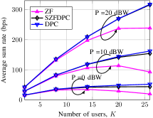
Figure 1: Average sum rate versus the number of users for MIMO systems with PAPC, $N=64$ transmit antennas.

Since Algorithm 2 and other benchmark scheme of consideration all generate the optimal solution to the corresponding problem, we mainly compare their complexity. In particular, we compare the runtime of Algorithm 2 with the interior-point method proposed in [8]. Fig. 2 plots the average runtime as a function of the number of transmit antennas $N$ for finding the maximum sum rate of SZFDPC. We observe that Algorithm 2 performs water-filling and GP to find $\bar{\mathbf{S}},\mathbf{Q}$, which results in lower computation time compared with [8] which uses the barrier interior-point method. In general, the barrier method and other second-order optimization methods are known to achieve a superlinear rate but its per-iteration cost increases quickly with the problem size. This is actually consistent with what is shown in Fig. 2 for the barrier-method [8].

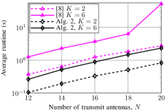
Figure 2: Runtime versus the number of transmit antennas for solving the sum rate maximization problem with SZFDPC scheme. Two methods are compared: Algorithm 2, and the interior-point method in [8].

As can be seen from Fig. 2, our AO-based algorithm, though has low complexity, may take a few seconds or more to execute when we increase the problem size. Thus, a method of lower complexity which can strike a balance between the sum rate and complexity is of interest. In the following, we will investigate the performance of our ML-based approach to such scenarios. The PAPC ratio is chosen randomly, whereas SNR is chosen from the set $\textrm{SNR}=[0,10,20,30,40]$ dBW. For each MIMO setting we generated 240 samples. Also, we simply use natural log to transform the feature space in (13).

In Fig. 3, we compare the optimal and estimate sum rates of a MIMO system with linear and nonlinear regression methods. More specifically, we utilize support vector regression (SVR) with radial basis function (RBF) kernel [23] for nonlinear regression. Here, we train on 216 samples and test on 24 samples. As can be seen from the figure, without proper preprocessing methods both OLS and SVR fail to fit the data due to nonlinear nature of the problem. However, the results of the simple OLS, which take feature design into account, are very close to optimal solutions. The performance has also proved the feasibility of our approach.

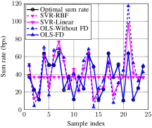
Figure 3: Sum rate estimate of linear and nonlinear regressions with and without feature design approach, $N=32$ transmit antennas, $M=2$ receive antennas and $K=2$ users.

In the last experiment, we consider the effectiveness of our approach in terms of average relative root mean square error (aRRMSE) [24] over large samples with varying number of transmit and receive antennas. In particular, we obtain the aRRMSE by executing 10-fold cross-validation using three simple linear ML algorithms: OLS, Ridge and PCR. According to [24], a learning model is considered good and excellent when $10\%<\textrm{aRRMSE}<20\%$ and $\textrm{aRRMSE}<10\%$, respectively. Interestingly, the ML-based method shows a sufficiently low error rate, especially when $\frac{N}{K}\geq 10$. From our observations, the training matrices are invertible and the eigenvalues are larger than 1, thus the performance of OLS and PCR is the same and has minor difference in comparison with that of ridge regression. Unsurprisingly, this observation coincides with the properties of these regression methods.

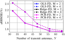
Figure 4: aRRMSE of OLS, Ridge regression and PCR with feature design and $K=2$ users.

V Conclusions

We have proposed two low-complexity methods to compute sum rates of MIMO systems under PAPC and SZFDPC. The experiments using the optimal approach have stated that the SZFDPC can obtain near-capacity rates whereas the ZF scheme still operates far from the optimal capacity boundary for a specified number of users. The suboptimal ML-based method is more advantageous in case of large-scale MIMO settings. Extensive numerical results have demonstrated the superiority of the proposed algorithms over the existing interior-point method. More importantly, our ML-based approach can be applicable to a class of similar problems.

References

- [1] E. Telatar, “Capacity of multi-antenna Gaussian channels,” Eur. Trans. Telecommun, vol. 10, pp. 585–598, Nov. 1999.
- [2] G. J. Foschini and M. J. Gans, “On limits of wireless communications in a fading environment when using multiple antennas,” Wireless Pers.Commun, vol. 6, pp. 311–335, Mar. 1998.
- [3] H. Weingarten, Y. Steinberg, and S. S. Shamai, “The capacity region of the Gaussian multiple-input multiple-output broadcast channel,” IEEE Trans. Inf. Theory, vol. 52, no. 9, pp. 3936 – 3964, Sep. 2006.
- [4] G. Caire and S. Shamai, “On the achievable throughput of a multiantenna Gaussian broadcast channel,” IEEE Trans. Inf. Theory, vol. 49, no. 7, pp. 1691–1706, Jul. 2003.
- [5] A. Dabbagh and D. Love, “Precoding for multiple antenna Gaussian broadcast channels with successive zero-forcing,” IEEE Trans. Signal Process., vol. 55, no. 7, pp. 3837–3850, Jul. 2007.
- [6] Q. Spencer, A. Swindlehurst, and M. Haardt, “Zero-forcing methods for downlink spatial multiplexing in multiuser MIMO channels,” IEEE Trans. Signal Process., vol. 52, no. 2, pp. 461–471, Feb. 2004.
- [7] T. M. Pham, and R. Farrell, and J. Dooley, and E. Dutkiewicz, and D. N. Nguyen, and L.-N. Tran, “Efficient zero-forcing precoder design for weighted sum-rate maximization with per-antenna power constraint,” IEEE Trans. Veh. Technol., vol. 67, no. 4, pp. 3640–3645, Apr. 2018.
- [8] L.-N. Tran, M. Juntti, M. Bengtsson, and B. Ottersten, “Weighted sum rate maximization for MIMO broadcast channels using dirty paper coding and zero-forcing methods,” IEEE Trans. Commun., vol. 61, no. 6, pp. 2362–2373, Jun. 2013.
- [9] ——, “Beamformer designs for MISO broadcast channels with zero-forcing dirty paper coding,” IEEE Trans. Wireless Commun., vol. 12, no. 3, pp. 1173–1185, Mar. 2013.
- [10] W. Yu, W. Rhee, S. Boyd, and J. Cioffi, “Iterative water-filling for Gaussian vector multiple-access channels,” IEEE Trans. Inf. Theory, vol. 50, no. 1, pp. 145–152, Jan. 2004.
- [11] N. Jindal, W. Rhee, S. Vishwanath, S. Jafar, and A. Goldsmith, “Sum power iterative water-filling for multi-antenna Gaussian broadcast channels,” IEEE Trans. Inf. Theory, vol. 51, no. 4, pp. 1570–1580, Apr. 2005.
- [12] J. Liu, Y. T. Hou, and H. D. Sherali, “On the maximum weighted sum-rate of MIMO Gaussian broadcast channels,” in Proc. IEEE ICC, May 2008, pp. 3664 – 3668.
- [13] M. Vu, “MIMO capacity with per-antenna power constraint,” in Proc. IEEE GLOBECOM, Dec. 2011, pp. 1 – 5.
- [14] W. Yu and T. Lan, “Transmitter optimization for the multi-antenna downlink with per-antenna power constraints,” IEEE Trans. Signal Process., vol. 55, no. 6, pp. 2646–2660, Jun. 2007.
- [15] T. M. Pham, and R. Farrell, and L.-N. Tran, “Low-complexity approaches for MIMO capacity with per-antenna power constraint,” in Proc. IEEE VTC-Spring, Jun. 2017, pp. 1–7.
- [16] ——, “Alternating optimization for capacity region of Gaussian MIMO broadcast channels with per-antenna power constraint,” in Proc. IEEE VTC-Spring, Jun. 2017, pp. 1–6.
- [17] L.-N. Tran and E.-K. Hong, “Multiuser diversity for successive zero-forcing dirty paper coding: Greedy scheduling algorithms and asymptotic performance analysis,” IEEE Trans. Signal Process., vol. 58, no. 6, pp. 3411–3416, Jun. 2010.
- [18] S. Vishwanath, N. Jindal, and A. Goldsmith, “Duality, achievable rates and sum-rate capacity of Gaussian MIMO broadcast channels,” IEEE Trans. Inf. Theory, vol. 49, pp. 2658–2668, Oct. 2003.
- [19] L. Armijo, “Minimization of functions having Lipschitz continuous first partial derivatives.” Pacific J. Math., vol. 16, no. 1, pp. 1 – 3, 1966.
- [20] L. Condat, “Fast projection onto the simplex and the ball,” Mathematical Programming, Series A, vol. 158, no. 1, pp. 575 – 585, Jul. 2016.
- [21] F. Song, Z. Guo, and D. Mei, “Feature selection using principal component analysis,” in Proc. IEEE ICSEM, vol. 1, Nov. 2010, pp. 27–30.
- [22] S. Theodoridis, Machine Learning: A Bayesian and Optimization Perspective, 1st ed. Orlando, FL, USA: Academic Press, Inc., 2015.
- [23] A. J. Smola and B. Schölkopf, “A tutorial on support vector regression,” Statistics and Computing, vol. 14, no. 3, pp. 199–222, Aug. 2004.
- [24] M.-F. Li, X.-P. Tang, W. Wu, and H.-B. Liu, “General models for estimating daily global solar radiation for different solar radiation zones in mainland china,” Energy Conversion and Management, vol. 70, pp. 139 – 148, 2013.