Integrated conditional moment test and beyond: when the number of covariates is divergent

Abstract

The classic integrated conditional moment test is a promising method for testing model misspecification. However, we show in this paper its failure in high dimensionality scenarios. To extend it to handle the testing problem with diverging number of covariates, we investigate three issues in inference in this paper. First, we study the consistency and asymptotically linear representation of the least squares estimator of the parameter at the fastest rate of divergence in the literature for nonlinear models. Second, we propose a projected adaptive-to-model version of the integrated conditional moment test in the diverging dimension scenarios. We study the asymptotic properties of the new test under both the null and alternative hypothesis to examine its ability of significance level maintenance and its sensitivity to the global and local alternatives that are distinct from the null at the fastest possible rate in hypothesis testing. Third, we derive the consistency of the bootstrap approximation for the null distribution in the diverging dimension setting. The numerical studies show that the new test can very much enhance the performance of the original ICM test in high-dimensional cases. We also apply the test to a real data set for illustrations.

Key words: Adaptive-to-model test, dimension reduction, integrated conditional moment test, least squares estimation, model checking, projection-based technique.

1 Introduction

Testing for model specification is one of the most important issues in regression analysis because using a misspecified regression model in practice may induce misleading statistical inference. Relevant theories for such inference problems have been rather mature when the dimension $p$ of predictor vector is fixed. However, in high dimensional data analysis, for large $p$ that should be treated as a divergent number when the sample size $n$ tends to infinity, such model checking problems have not yet been systematically studied in the literature. Thus the research described in this paper is motivated by developing a goodness-of-fit test for parametric multiple-index regression models in the diverging dimension settings. As everything in this paper relies on the sample size $n$, we stress $n$ in the notations.

We begin with describing the model checking problem in detail. Let $Y$ represent the real-valued response variable and let $X\in\mathbb{R}^{p}$ be its associated random-design predictor vector. The null hypothesis we want to test is that $(Y,X)$ follows a parametric multiple-index model as

$$Y=g(\beta_{10}^{\top}X,\cdots,\beta_{d0}^{\top}X,\vartheta_{0})+\varepsilon$$ (1.1)

where $g$ is a given smooth function, $\vartheta_{0}\in\mathbb{R}^{l}$ and $\bm{\beta}_{0}=(\beta_{10},\cdots,\beta_{d0})\in\mathbb{R}^{p\times d}$ are the unknown matrix of regression parameters, $\varepsilon=Y-E(Y|X)$ is the unpredictable part of $Y$ given $X$, and the notation $\top$ denotes the transpose. Without loss of generality, we assume that $\beta_{10},\cdots,\beta_{d0}$ are orthogonal. To make full use of the model structure under both the null and the alternative hypothesis, consider the following general alternative model

$$Y=G(\bm{B}^{\top}X)+\varepsilon,$$ (1.2)

where $E(\varepsilon|X)=0$, $G(\cdot)$ is an unknown smooth function, and $\bm{B}$ is a $p\times q$ orthonormal matrix such that $\mathcal{S}_{E(Y|X)}={\rm span}(\bm{B})$. Here $\mathcal{S}_{E(Y|X)}$ is the central mean space of $Y$ with respect to $X$ which will be specified in Section 4.

When the dimension $p$ of predictor vector is fixed, there are a number of proposals in the literature for testing the parametric regression models consistently which can also be applied to test the null hypothesis of model (1.1). We just list a few such as Härdle and Mammen (1993), Zheng (1996), Dette (1999), Fan and Huang (2001), Horowitz and Spokoiny (2001), Koul and Ni (2004), van Keilegom et al. (2008) and Lavergne and Patilea (2008, 2012) by using nonparametic estimation methods. They are called local smoothing tests. Some of tests in this class have tractable limiting null distributions, but the use of nonparametric regression estimations usually causes them to suffer severely from the curse of dimensionality in high-dimensional cases. Guo et al. (2016) gave some detailed comments on this issue. The empirical process-based tests are constructed in terms of converting conditional expectations $E(\varepsilon|X)=0$ to infinite and parametric unconditional orthogonality restrictions, that is

$$E(\varepsilon|X)=0\quad\Leftrightarrow\quad E[\varepsilon w(X,t)]=0\quad\forall\ t\in\Gamma,$$ (1.3)

where $\Gamma$ is some proper space. There exist several parametric families $w(X,t)$ such that the equivalence (1.3) holds; see Bierens and Ploberger (1997) and Escanciano (2006b) for more details on the primitive conditions of $w(\cdot,t)$ to satisfy this equivalence. The indicator function $w(X,t)=I(X\leq t)$ is commonly used as a weight function in the literature; see, e.g., Stute (1997), Stute, Gonz$\rm\acute{a}$lez Manteiga and Presedo Quindimil (1998), Stute, Thies and Zhu (1998), Zhu (2003), Khmadladze and Koul (2004), Stute, Xu and Zhu (2008), among many others.

In a seminal paper, Bierens (1982) used the characteristic function $w(X,t)=\exp(\mathrm{i}t^{\top}X)$ as the weight function and constructed an integrated conditional moment (ICM) test, where $\mathrm{i}=\sqrt{-1}$ denotes the imaginary unit. The ICM test statistic is given by

$$ICM_{n}=\int_{\Gamma}|\frac{1}{\sqrt{n}}\sum_{j=1}^{n}\hat{\eta}_{j}\exp(\mathrm{i}t^{\top}\Phi(X_{j}))|^{2}d\mu(t),$$ (1.4)

where $\hat{\eta}_{j}$ is the residual, $\Gamma=\prod_{i=1}^{p}[-\epsilon_{i},\epsilon_{i}]$ where $\epsilon_{i}$ are arbitrarily positive numbers, $\mu$ is the Lebesgue measure on $\Gamma$, and $\Phi(\cdot)$ is an one-to-one bounded smoothing function from $\mathbb{R}^{p}$ to $\mathbb{R}^{p}$. Note that Bierens’ original test statistic $ICM_{n}$ integrates over a compact subset $\Gamma\subset\mathbb{R}^{p}$. It is well known that high-dimensional numerical integrations are extremely difficult to handle in practice. When $p$ is large, the computation of the integral in (1.4) or its approximation becomes difficult and time consuming. Thus it is usually suggested in the literature to use the standard normal measure and integrating over the whole space $\mathbb{R}^{p}$ in (1.4). See Escanciano (2006a), Lavergne and Patilea (2008, 2012). Then the high-dimensional numerical integrations can be avoided and Bierens’ test statistic becomes

$$ICM_{n}=\int_{\mathbb{R}^{p}}|\frac{1}{\sqrt{n}}\sum_{j=1}^{n}\hat{\eta}_{j}\exp(\mathrm{i}t^{\top}X_{j}))|^{2}\phi(t)dt=\frac{1}{n}\sum_{j,k=1}^{n}\hat{\eta}_{j}\hat{\eta}_{k}\exp(-\frac{1}{2}\|X_{j}-X_{k}\|^{2}),$$ (1.5)

where $\phi(t)$ denotes the standard normal density on $\mathbb{R}^{p}$. Note that the ICM test statistic is not asymptotically distribution-free and thus it needs to resort resampling methods to approximate the null distribution to determine the critical value. When the dimension $p$ is fixed, Stute, Gonz$\acute{a}$lez Manteiga and Presedo Quindimil (1998) first showed that the distribution of residual marked empirical processes can be approximated by the wild bootstrap. Dominguez (2004) further proved the validity of the wild bootstrap for the ICM test in the fixed dimension setting. However, when the dimension $p$ is divergent as the sample size $n$ tends to infinity, we find that the limiting distributions of $ICM_{n}$ can be completely different from the classic results in the fixed dimension setting. Under mild conditions, we show that $ICM_{n}$ could degenerate to finite fixed values under both the null and alternative hypotheses. We further show that the wild bootstrap version of the ICM test statistic also has the exact same limits as $ICM_{n}$ under underlying models, rather than approximates the null distribution. These results are presented in Section 3 below. Therefore, this could cause the lack of power of the ICM test in the large dimension scenarios when using the wild bootstrap. The simulation results in Section 6 show that the ICM test based on the wild bootstrap completely breaks down for large dimension $p$.

The primary purpose of this research is to extend the Bierens’ (1982) ICM test to the diverging dimension setting and simultaneously avoid the dimensionality problem under the multiple index model structure. We notice that the main reason that the ICM test based on the wild bootstrap fails to work is that the weight function $\exp(-\|X_{j}-X_{k}\|^{2}/2)$ in (1.5) degenerates to zero at an exponential rate when the dimension $p$ tends to infinity. In order to overcome this difficulty, we adopt projection pursuit and sufficient dimension reduction (SDR) techniques to reduce the original dimension $p$ to a much lower dimension and then develop a projected adaptive-to-model version of the $ICM_{n}$ test in diverging dimension cases. The asymptotic properties of the proposed test are investigated under both the null and alternative hypothesis when $p$ is divergent. We show that the proposed test has a non-degenerate limiting null distribution, is consistent against any alternative hypothesis, and can detect the local alternatives converging to the null at the parametric rate $1/\sqrt{n}$ in the diverging dimension scenario. Although the ICM test based on the wild bootstrap fails to work in diverging dimension settings, we show that the proposed test can still be approximated by the wild bootstrap provided $p=o(n/\log{n})^{1/3}$.

Note that the innovative model adaptation methodology is first proposed by Guo et al. (2016) for testing the specification of parametric single index models in the fixed dimension cases. To make sure that their test is omnibus, they imposed a restrictive assumption on the central mean subspace $\mathcal{S}_{E(Y|X)}$ which may not hold for nonlinear regression models. In this paper we modify the model adaptation procedure to remove this annoying assumption and extend it to handle the model checking problems for multiple index models. More details about this issue will be given in Section 4. Tan and Zhu (2019a) also used the methodology to attack the same testing problem with diverging dimension $p$. However, for multiple-index null models, Tan and Zhu’s (2019a) test does not work and is not extendable to handle such models as in general the martingale transformation developed there fails to work.

This paper also concerns with studying the asymptotic properties of the estimator $(\bm{\hat{\beta}},\hat{\vartheta})$ of $(\bm{\beta}_{0},\vartheta_{0})$ in the divergent dimension cases, as we need the residuals to construct the test statistic. This problem has been well investigated for linear regression models, see Huber (1973), Portnoy (1984, 1985) and Zou and Zhang (2009), etc. Nevertheless, for nonlinear models, it has rarely been studied in the literature. Under some mild conditions, Tan and Zhu (2019a) obtained the estimation consistency and the asymptotically linear representation of $(\bm{\hat{\beta}},\hat{\vartheta})$ at the rates $p=o(n^{1/4})$ and $p=o(n^{1/5})$ of divergence respectively. In this paper, with the help of some high dimensional empirical processes techniques developed in Tan and Zhu (2019b), we will greatly improve these rates of divergence to $p=o(n^{1/2})$ and $p=o(n/\log n)^{1/3}$ and obtain the uniformly asymptotically linear representation of $(\bm{\hat{\beta}},\hat{\vartheta})$. These improvements enhance our ability to handle higher dimension in model checking problems. Under the conditions we design, the rates are the best in the relevant research in the literature to the best of our knowledge. Shi et al. (2019) obtained similar results for generalized linear models with fixed design in the divergent dimension setting. But, as we actually deal with general nonlinear models with random design here, their approach is significantly different from ours.

The rest of this article is organised as follows. In Section 2 we present the asymptotic results of the least squares estimation of the parameters in diverging dimension scenarios. In Section 3, we studies the limiting properties of the ICM test and its wild bootstrap version in the diverging dimension setting. Section 4 describes the basic test construction. Since sufficient dimension reduction techniques are crucial for the model adaptation property, we give a short review in this section. To alleviate the computational complexity of the test statistic, we also discuss the choice of the weight functions in this section. Section 5 is devoted to present the asymptotic properties of the test under both the null and alternatives. The bootstrap approximation to the null distribution of the test statistic is used and its validity in the diverging dimension setting is verified in this section. In Section 6, the simulation results are reported and a real data analysis is used as an illustration of application. Section 7 contains some discussions and topics for future study. The discussion of the regularity conditions and technical proofs of the theoretical results are contained in Supplementary Material for saving space.

2 Parametric estimation

In this section, we consider the parameter estimation for model (1.1), and also study its asymptotic properties in the diverging dimension setting. Recall the null model (1.1)

$$Y=g(\bm{\beta}_{0}^{\top}X,\vartheta_{0})+\varepsilon.$$

To estimate the unknown parameters $(\bm{\beta}_{0},\vartheta_{0})$, we here restrict ourselves to the ordinary least squares method. For notational simplicity, define $\theta=[vec(\bm{\beta})^{\top},\vartheta^{\top}]^{\top}$ where $vec(\bm{\beta})=[\beta_{1}^{\top},\cdots,\beta_{d}^{\top}]^{\top}$. Then we rewrite the null hypothesis $H_{0}$ in the following parametric regression format:

$$H_{0}:Y=g(\theta_{0},X)+\varepsilon\quad{\rm for\ some}\ \theta_{0}\in\Theta\subset\mathbb{R}^{m},$$

where $m=pd+l$, $E(\varepsilon|X)=0$ and $\Theta$ is a compact subset of $\mathbb{R}^{m}$. Next we consider the ordinary least squares estimator of $\theta_{0}$ and its asymptotic properties. Let

$$\hat{\theta}=\mathop{\rm arg\ min}\limits_{\theta\in\Theta}\sum_{i=1}^{n}[Y_{i}-g(\theta,X_{i})]^{2}.$$ (2.1)

To analyse the asymptotic properties of $\hat{\theta}$, set

$$\tilde{\theta}_{0}=\mathop{\rm arg\ min}\limits_{\theta\in\Theta}E[Y-g(\theta,X)]^{2}=\mathop{\rm arg\ min}\limits_{\theta\in\Theta}E[m(X)-g(\theta,X)]^{2},$$ (2.2)

where $m(x)=E(Y|X=x)$ denotes the regression function. Under the regularity condition (A4) specified below, $\tilde{\theta}_{0}=\theta_{0}$ under the null hypothesis. Under the alternatives, $\tilde{\theta}_{0}$ typically depends on the cumulative distribution of $X$. We now state the regularity conditions under which we can derive the asymptotic properties of $\hat{\theta}$ when the dimension $m$ is divergent.

(A1). The function $g(\theta,x)$ admits third derivatives in $\theta$ and putting

$$g^{\prime}(\theta,x)=\frac{\partial g(\theta,x)}{\partial\theta},\ g_{j}^{{}^{\prime}}(\theta,x)=\frac{\partial g(\theta,x)}{\partial\theta_{j}},\ {\rm and}\ g_{jk}^{{}^{\prime\prime}}(\theta,x)=\frac{\partial^{2}g(\theta,x)}{\partial\theta_{j}\partial\theta_{k}}.$$

Further, (i) $E(Y^{4})<\infty$; (ii) $|g(\theta,x)|\leq F(x)$, $|g_{j}^{{}^{\prime}}(\theta,x)|\leq F(x)$ and $|g_{jk}^{{}^{\prime\prime}}(\theta,x)|\leq F(x)$ for all $j,k=1,\cdots,m$ and $\theta\in U(\tilde{\theta}_{0})$, where $F(x)$ is a measurable function such that $E|F(X)|^{4}=O(1)$ and $U(\tilde{\theta}_{0})$ is some neighborhood of $\tilde{\theta}_{0}$.

(A2). Let $\psi(\theta,x)=[m(x)-g(\theta,x)]g^{\prime}(\theta,x)$ and $P\dot{\psi}_{\theta}=E\{\frac{\partial\psi}{\partial\theta^{\top}}(\theta,X)\}.$ Define $\Sigma=-P\dot{\psi}_{\tilde{\theta}_{0}}$. The matrix $\Sigma$ is nonsingular with

$$0<\underline{\lambda}\leq\lambda_{\min}(\Sigma)\leq\lambda_{\max}(\Sigma)<\overline{\lambda}<\infty,$$

where $\underline{\lambda}$ and $\overline{\lambda}$ are two constants that do not depend on $n$ and $\lambda_{\min}(\Sigma)$ and $\lambda_{\max}(\Sigma)$ denote the smallest and largest eigenvalue of $\Sigma$ respectively.

(A3) Let $\psi_{j}(\theta,x)=[m(x)-g(\theta,x)]g_{j}^{\prime}(\theta,x)$ and $P\ddot{\psi}_{j\theta}=E\{\frac{\partial^{2}\psi_{j}}{\partial\theta\partial\theta^{\top}}(\theta,X)\}$. The matrix $P\ddot{\psi}_{j\theta}$ satisfies

$$\max_{1\leq i,j\leq m}|\lambda_{i}(P\ddot{\psi}_{j\theta})|\leq C,\quad\forall\ \theta\in U(\tilde{\theta}_{0}),$$

where $C$ is a constant free of $n$ and $\{\lambda_{i}(P\ddot{\psi}_{j\theta}):1\leq i\leq m\}$ are the eigenvalues of the matrix $P\ddot{\psi}_{j\theta}$.

(A4). The vector $\tilde{\theta}_{0}$ lies in the interior of the compact subset $\Theta$ and is the unique minimizer of (2.2).

(A5). Putting $\psi^{{}^{\prime\prime}}_{jkl}(\theta,x)=\frac{\partial^{2}\psi_{j}}{\partial\theta_{k}\partial\theta_{l}}(\theta,x)$ and $g^{{}^{\prime\prime\prime}}_{jkl}(\theta,x)=\frac{\partial^{3}g}{\partial\theta_{j}\partial\theta_{k}\partial\theta_{l}}(\theta,x)$. For every $\theta_{1}$ and $\theta_{2}$ in the neighborhood $U(\tilde{\theta}_{0})$ of $\tilde{\theta}_{0}$,

$$|\psi^{{}^{\prime\prime}}_{jkl}(\theta_{1},x)-\psi^{{}^{\prime\prime}}_{jkl}(\theta_{2},x)|\leq\sqrt{m}\|\theta_{1}-\theta_{2}\|F_{1}(x),$$

$$|g^{{}^{\prime\prime\prime}}_{jkl}(\theta_{1},x)-g^{{}^{\prime\prime\prime}}_{jkl}(\theta_{2},x)|\leq\sqrt{m}\|\theta_{1}-\theta_{2}\|F_{2}(x),$$

where $F_{1}(x)$ and $F_{2}(x)$ are two measurable functions satisfying that $E|F_{1}(X)|^{4}=O(1)$ and $E|F_{2}(X)|^{8}=O(1)$.

The regularity conditions (A1) and (A4) are standard for the nonlinear least squares estimation, see, e.g., Jennrich (1969) and White (1981). Condition (A2) is similar to the regularity condition (F) imposed on the information matrix $I_{n}$ of the likelihood function in Fan and Peng (2004) which facilitates the theoretical derivations. Condition (A3) is necessary for controlling the convergence rate of the remainder term in deriving the asymptotic properties of $\tilde{\theta}_{0}$. In Section 1 of the Supplementary Material, we will show that this condition holds for multiple-index regression models if the predictor vector $X$ admits an appropriate multivariate distribution. Condition (A5) is needed for obtaining the uniformly asymptotically linear representation of $\hat{\theta}-\tilde{\theta}_{0}$. Although we only need the asymptotic properties of the parameters for multiple index models in this paper, the asymptotic properties of $\tilde{\theta}_{0}$ also hold for general parametric regression models.

Theorem 2.1.

Suppose that the regularity conditions (A1)-(A4) hold. If $m^{2}/n\to 0$, then it follows that $\hat{\theta}$ is a norm consistent estimator of $\tilde{\theta}_{0}$ in the sense that $\|\hat{\theta}-\tilde{\theta}_{0}\|=O_{p}(\sqrt{m/n})$ where $\|\cdot\|$ denotes the Frobenius norm. Furthermore, if $(m^{3}\log{n})/n\to 0$, then under the regularity conditions (A1)-(A5),

$$\sqrt{n}\alpha^{\top}(\hat{\theta}-\tilde{\theta}_{0})=\frac{1}{\sqrt{n}}\sum_{i=1}^{n}[Y_{i}-g(\tilde{\theta}_{0},X_{i})]\alpha^{\top}\Sigma^{-1}g^{\prime}(\tilde{\theta}_{0},X_{i})+o_{p}(1),$$ (2.3)

where the remaining term $o_{p}(1)$ is uniform in $\alpha\in\mathcal{S}^{m-1}$ and $\mathcal{S}^{m-1}$ is the unit sphere in $\mathbb{R}^{m}$.

The convergence rate $O_{p}(\sqrt{m/n})$ in Theorem 2.1 is in line with the results of the $M$-estimator studied by Huber (1973) and Portnoy (1984) when the number of parameters is divergent. But they only considered linear regression models $g(\theta,X)=\theta^{\top}X$. In Theorem 2.1 we also obtain the uniformly asymptotically linear representation of $\hat{\theta}-\tilde{\theta}$. This result is much stronger than that in Portnoy (1985) who obtained the linear representation for a given $\alpha\in\mathcal{S}^{m-1}$ in linear regression models. Furthermore, in the linear regression setting and the sub-Gaussian cases, we can derive, when $p=o(n)$ and $p=o(n^{1/2})$, the norm consistency and the uniformly asymptotically linear representation of $\hat{\theta}$ to $\tilde{\theta}_{0}$. Here we say a random variable $Z\in\mathbb{R}$ is sub-Gaussian with variance proxy $\sigma^{2}$ if

$$E\{\exp[u(Z-EZ)]\}\leq\exp(\frac{\sigma^{2}u^{2}}{2}),\ \forall\ u\in\mathbb{R}.$$

A random vector $X\in\mathbb{R}^{p}$ is sub-Gaussian with variance proxy $\sigma^{2}$ if $v^{\top}X$ is sub-Gaussian with variance proxy $\sigma^{2}$ for all $v\in\mathcal{S}^{p-1}$.

Theorem 2.2.

Suppose that the regularity conditions (A1)-(A4) hold for linear regression models and $X$ is sub-Gaussian with the variance proxy $\sigma^{2}$. If $p/n\to 0$, then we have $\|\hat{\theta}-\tilde{\theta}_{0}\|=O_{p}(\sqrt{p/n})$ where $\|\cdot\|$ denotes the Frobenious norm. Moreover, if $p^{2}/n\to 0$, it follows that

$$\sqrt{n}\alpha^{\top}(\hat{\theta}-\tilde{\theta}_{0})=\frac{1}{\sqrt{n}}\sum_{i=1}^{n}(Y_{i}-\tilde{\theta}_{0}^{\top}X_{i})\alpha^{\top}\Sigma^{-1}X_{i}+o_{p}(1),$$

where $\Sigma=E(XX^{\top})$ and the term $o_{p}(1)$ is uniform in $\alpha\in\mathcal{S}^{p-1}$.

3 The ICM test and the wild bootstrap in diverging dimension settings

It is well known that the ICM test is not asymptotically distribution-free since its limiting null distribution relies on the unknown Data Generating Process. Thus the wild bootstrap is usually adopted in the literature to approximate the asymptotically null distribution of the ICM test statistic. See Stute, Gonz$\acute{a}$lez Manteiga and Presedo Quindimil (1998) and Dominguez (2004). However, when the dimension $p$ is divergent as the sample size $n$ tends to infinity, we will show that the wild bootstrap does not work for the ICM test. To see this, recall that the ICM test can be restated as

$$ICM_{n}=\frac{1}{n}\sum_{j,k=1}^{n}\hat{\eta}_{j}\hat{\eta}_{k}\exp(-\frac{1}{2}\|X_{j}-X_{k}\|^{2})=\frac{1}{n}\sum_{j}^{n}\hat{\eta}_{j}^{2}+\frac{2}{n}\sum_{j<k}\hat{\eta}_{j}\hat{\eta}_{k}\exp(-\frac{1}{2}\|X_{j}-X_{k}\|^{2}),$$

where $\hat{\eta}_{j}=Y_{j}-g(\hat{\theta},X_{j})$. Assuming that the regularity conditions (A1)-(A5) hold, we can show that under the null hypothesis,

$$ICM_{n}=E(\varepsilon^{2})+O_{p}(\sqrt{p^{2}/n})+p^{2}\{E[\exp(-2\|X_{1}-X_{2}\|^{2})]\}^{1/4}O_{p}(1).$$ (3.1)

While under the alternative hypothesis, we have

$$ICM_{n}=E[\varepsilon+m(X)-g(\tilde{\theta}_{0},X)]^{2}+O_{p}(\sqrt{p^{2}/n})+n\{E[\exp(-\|X_{1}-X_{2}\|^{2})]\}^{1/2}O_{p}(1).$$ (3.2)

The proofs for (3.1) and (3.2) are given in the Supplementary Material (Lemma 2). Note that the convergence rates obtained in (3.1) and  (3.2) coincide with the classic asymptotic results of the ICM test statistic in fixed dimension scenarios. However, if $p$ diverges as the sample size $n$ tends to infinity, we will see that the classic limiting results of $ICM_{n}$ completely break down. To better understand this phenomenon in the diverging dimension setting, we take a special case for illustration. Suppose that the components $\{X_{1k}:k=1,\cdots,p\}$ of $X_{1}$ are independent and identically distributed. It is readily seen that

$$E[\exp(-2\|X_{1}-X_{2}\|^{2})]=\{E[\exp(-2|X_{11}-X_{21}|^{2})]\}^{p}.$$

This means $E[\exp(-2\|X_{1}-X_{2}\|^{2})]$ converges to zero at an exponential rate. If $p^{2}/n\to 0$ and $(\log{n})/p\to 0$, it is easy to see that $ICM_{n}$ converges to finite points under both the null and alternative hypotheses.

Now we can show that the wild bootstrap that has been used to the ICM test completely break down when the dimension $p$ is divergent. The procedure of the wild bootstrap is as follows. Set

$$X_{j}^{*}=X_{j}\quad{}\quad Y_{j}^{*}=g(\hat{\theta},X_{j})+\hat{\eta}_{j}V_{j}^{*},j=1,\cdots,n,$$

where $\hat{\eta}_{j}$ is the residual and $\{V_{j}^{*}\}_{j=1}^{n}$ are i.i.d. bounded random variables with zero mean and unit variance, independent of the original sample $\{(X_{i},Y_{i})\}_{j=1}^{n}$. An often used example of $\{V_{j}^{*}\}_{j=1}^{n}$ is the i.i.d. Bernoulli variates with

$$\mathbb{P}(V_{j}^{*}=\frac{1-\sqrt{5}}{2})=\frac{1+2\sqrt{5}}{2\sqrt{5}},\quad\mathbb{P}(V_{j}^{*}=\frac{1+\sqrt{5}}{2})=1-\frac{1+2\sqrt{5}}{2\sqrt{5}}.$$

For other examples of $\{V_{j}^{*}\}_{j=1}^{n}$, one can refer to Mammen (1993). Let $\hat{\theta}^{*}$ be the bootstrap estimator obtained by the ordinary least square based on the bootstrap sample $\{(X_{j},Y_{j}^{*})\}_{j=1}^{n}$. Then the bootstrap version of the ICM test statistic is given by

$$ICM^{*}_{n}=\int_{\mathbb{R}^{p}}|\frac{1}{\sqrt{n}}\sum_{j=1}^{n}\hat{\eta}^{*}_{j}\exp(\mathrm{i}t^{\top}X_{j}))|^{2}\phi(t)dt=\frac{1}{n}\sum_{j,k=1}^{n}\hat{\eta}^{*}_{j}\hat{\eta}^{*}_{k}\exp(-\frac{1}{2}\|X_{j}-X_{k}\|^{2}),$$ (3.3)

where $\hat{\eta}^{*}_{j}=Y^{*}_{j}-g(\hat{\theta}^{*},X_{j})$ and $\phi(t)$ is the standard normal density in $\mathbb{R}^{p}$.

Let $P^{*}$ be the probability measure induced by the wild bootstrap resampling conditional on the original sample $\{(X_{i},Y_{i}):i=1,\cdots,n\}$. Then under the regularity conditions (A1)-(A5), we can show that

$$ICM_{n}^{*}=E[\varepsilon+m(X)-g(\tilde{\theta}_{0},X)]^{2}+O_{P^{*}}(\sqrt{p^{2}/n})+p^{2}\{E[\exp(-2\|X_{1}-X_{2}\|^{2})]\}^{1/4}O_{P^{*}}(1).$$ (3.4)

The proof of (3.4) is also given in the Supplementary Material (Lemma 3).

If the wild bootstrap is workable, the distribution of $ICM_{n}^{*}$ should well approximate the limiting null distribution of $ICM_{n}$. However, if $p^{2}/n\to 0$ and $(\log{n})/p\to 0$, it is readily seen that $ICM_{n}$ and its bootstrap version $ICM_{n}^{*}$ have the exact same limits under respectively the null and alternative hypothesis. Thus the wild bootstrap does not valid when the dimension $p$ is divergent. This indicates the lack of power of Bierens’ ICM test in large dimension scenarios when using the wild bootstrap. In Section 6, we conduct detailed simulation studies from small to large dimensions for Bierens’ ICM test based on the wild bootstrap. The simulation results also validate these phenomena.

4 Adaptive-to-model version of the ICM test

Now we restate the null hypothesis as

$$H_{0}:\ E(Y|X)=g(\bm{\beta}_{0}^{\top}X,\vartheta_{0})\quad{\rm for\ some}\ \bm{\beta}_{0}\in\mathbb{R}^{p\times d}\ {\rm and}\ \vartheta_{0}\in\mathbb{R}^{l}.$$

While the alternative hypothesis is that for any $\bm{\beta}\in\mathbb{R}^{p\times d}$ and $\vartheta\in\mathbb{R}^{l}$,

$$H_{1}:\ E(Y|X)=G(\bm{B}^{\top}X)\neq g(\bm{\beta}^{\top}X,\vartheta),$$

where $G$ is an unknown smoothing function, $\bm{B}$ is a $p\times q$ orthonormal matrix satisfying $\mathcal{S}_{E(Y|X)}={\rm span}(\bm{B})$. Here $\mathcal{S}_{E(Y|X)}$ is the central mean space of $Y$ with respect to $X$ which is defined as the intersection of all subspaces ${\rm span}(\bm{A})$ such that $Y\bot\!\!\!\bot E(Y|X)|\bm{A}^{\top}X$ where $\bot\!\!\!\bot$ means statistical independence and ${\rm span}(\bm{A})$ is the subspace spanned by the columns of $\bm{A}$. Under mild conditions, such a subspace $\mathcal{S}_{E(Y|X)}$ always exists (see Cook and Li (2002)). If $\mathcal{S}_{E(Y|X)}={\rm span}(\bm{B})$, it follows that $E(Y|X)=E(Y|\bm{B}^{\top}X)$. Thus it is reasonable to use the regression format $G(\bm{B}^{\top}X)$ instead of the fully nonparametric function $G(X)$ in the alternative hypothesis $H_{1}$. The dimension of $\mathcal{S}_{E(Y|X)}$ is called the structural dimension which is $q$ under the alternatives. Similarly, under the null we have $\mathcal{S}_{E(Y|X)}={\rm span}(\bm{B})={\rm span}(\bm{\beta_{0}})$ with a structural dimension $d$.

Recall that $\varepsilon=Y-E(Y|X)$ and

$$(\bm{\tilde{\beta}_{0}},\tilde{\vartheta}_{0})=\mathop{\rm arg\ min}\limits_{\bm{\beta}\in\mathbb{R}^{p\times d},\vartheta\in\mathbb{R}^{l}}E[Y-g(\bm{\beta}^{\top}X,\vartheta)]^{2}.$$

Let $\eta=Y-g(\bm{\tilde{\beta}_{0}}^{\top}X,\tilde{\vartheta}_{0})$ and $\bm{\tilde{\mathfrak{B}}}=(\bm{\tilde{\beta}_{0}},\bm{B})$. Under the null hypothesis, we have $\bm{\tilde{\beta}_{0}}=\bm{\beta_{0}}$ and ${\rm span}(\bm{B})=\rm{span}(\bm{\beta_{0}})$. Consequently,

$$E(\eta|\bm{\tilde{\mathfrak{B}}}^{\top}X)=E(Y|\bm{\tilde{\beta}_{0}}^{\top}X,\bm{B}^{\top}X)-g(\bm{\tilde{\beta}_{0}}^{\top}X,\tilde{\vartheta}_{0})=E(Y|\bm{\beta_{0}}^{\top}X)-g(\bm{\beta_{0}}^{\top}X,\vartheta_{0})=0.$$

Under the alternative, we have $\eta=G(\bm{B}^{\top}X)-g(\bm{\tilde{\beta}_{0}}^{\top}X,\tilde{\vartheta}_{0})+\varepsilon$. Then we obtain that

$$E(\eta|\bm{\tilde{\mathfrak{B}}}^{\top}X)=G(\bm{B}^{\top}X)-g(\bm{\tilde{\beta}_{0}}^{\top}X,\tilde{\vartheta}_{0})\neq 0.$$

By Theorem 1 of Bierens (1982), under the null, we have $E[\eta\exp(\mathrm{i}t^{\top}\bm{\tilde{\mathfrak{B}}}^{\top}X)]=0$ for all $t\in\mathbb{R}^{2d}$. Then it follows that

$$\int_{\mathbb{R}^{2d}}|E[\eta\exp(\mathrm{i}t^{\top}\bm{\tilde{\mathfrak{B}}}^{\top}X)]|^{2}\varphi(t)dt=0.$$ (4.1)

While under the alternative, there exist $t_{0}\in\mathbb{R}^{d+q}$ such that $E[\eta\exp(\mathrm{i}t_{0}^{\top}\bm{\tilde{\mathfrak{B}}}^{\top}X)]\neq 0$. Therefore,

$$\int_{\mathbb{R}^{d+q}}|E[\eta\exp(\mathrm{i}t^{\top}\bm{\tilde{\mathfrak{B}}}^{\top}X)]|^{2}\varphi(t)dt>0,$$ (4.2)

where $\varphi(t)$ denotes a positive weight function which will be specified later. Thereby we reject the null hypothesis for “large value” of the empirical version of the left-hand side of (3.1). Let $\{(X_{1},Y_{1}),\cdots,(X_{n},Y_{n})\}$ be a random sample from the distribution of $(X,Y)$. We then propose an adaptive-to-model integrated conditional moment test statistic as

$$\hat{V}_{n}(t)=\frac{1}{\sqrt{n}}\sum_{j=1}^{n}[Y_{j}-g(\bm{\hat{\beta}}^{\top}X_{j},\hat{\vartheta}_{0})]\exp(\mathrm{i}t^{\top}\bm{\hat{\mathfrak{B}}}^{\top}X_{j}),$$ (4.3)

$$AICM_{n}=\int_{\mathbb{R}^{d+\hat{q}}}|\hat{V}_{n}(t)|^{2}\varphi(t)dt,$$ (4.4)

where $\bm{\hat{\mathfrak{B}}}=(\bm{\hat{\beta}},\bm{\hat{B}})$, $\bm{\hat{B}}$ is a sufficient dimension reduction estimator of $\bm{B}$ with an estimated structural dimension $\hat{q}$ of $q$, and $\bm{\hat{\beta}}$ is a norm consistent estimators of $\bm{\tilde{\beta}_{0}}$. In this paper, we restrict ourselves to the least square estimator of $\bm{\tilde{\beta}_{0}}$.

It is worth mentioning that Guo et al. (2016) first used sufficient dimension reduction techniques to construct a goodness of fit test for parametric single-index models when the dimension $p$ of predictor vector is fixed. But they only used the matrix $\bm{B}$ rather than $(\bm{\tilde{\beta}_{0}},\bm{B})$ as we consider here. To make sure $E(\eta|{\bm{B}}^{\top}X)\neq 0$ under the alternative hypotheses, they need an extra condition that $\tilde{\beta}_{0}\in{\rm span}(\bm{B})$. Note that this restrictive condition does not always hold for nonlinear regression models. To avoid this extra condition, we use the matrix $\bm{\tilde{\mathfrak{B}}}$ in the test construction to ensure the conditional expectation $E(\eta|\bm{\tilde{\mathfrak{B}}}^{\top}X)\neq 0$ for all alternative hypotheses. Thus our new test is consistent for any alternative hypothesis.

4.1 The choice of $\varphi(t)$

The choice of weight functions $\varphi(t)$ is flexible. Recall that our test statistic $AICM_{n}=\int_{\mathbb{R}^{d+\hat{q}}}|\hat{V}_{n}(t)|^{2}\varphi(t)dt$. For any even positive function $\varphi(t)$, some elementary calculations lead to

$$AICM_{n} = \frac{1}{n}\int_{\mathbb{R}^{d+\hat{q}}}|\sum_{j=1}^{n}\hat{\eta}_{j}\exp(\mathrm{i}t^{\top}\bm{\hat{\mathfrak{B}}}^{\top}X_{j})|^{2}\varphi(t)dt$$

$$= \frac{1}{n}\sum_{j,k=1}^{n}\hat{\eta}_{j}\hat{\eta}_{k}\int_{\mathbb{R}^{d+\hat{q}}}\cos\{t^{\top}(\bm{\hat{\mathfrak{B}}}^{\top}X_{j}-\bm{\hat{\mathfrak{B}}}^{\top}X_{k})\}\varphi(t)dt$$

where $\hat{\eta}_{j}=Y_{j}-g(\bm{\hat{\beta}}^{\top}X_{j},\hat{\vartheta})$. Let $K_{\varphi}(x)=\int\cos(t^{\top}x)\varphi(t)dt$, then it follows that

$$AICM_{n}=\frac{1}{n}\sum_{j,k=1}^{n}\hat{\eta}_{j}\hat{\eta}_{k}K_{\varphi}(\bm{\hat{\mathfrak{B}}}^{\top}X_{j}-\bm{\hat{\mathfrak{B}}}^{\top}X_{k}).$$

Yet the calculation of $K_{\varphi}(x)$ is still complex in high dimension settings, even when we use sufficient dimension reduction techniques here. To facilitate the calculation of the test statistic, a close form of the function $K_{\varphi}(x)$ is preferred. There is a large class of weight functions $\varphi(t)$ available for this purpose. Consider the sub-Gaussian symmetric $a$-stable distribution as an example. By Proposition 2.5.2 of Samorodnitsky and Taqqu (1994), we have

$$K_{\varphi_{a}}(x)=\int_{\mathbb{R}^{p}}\cos(t^{\top}x)\varphi_{a}(t)dt=\exp(-|\frac{1}{2}\sum_{i,j=1}^{p}x_{i}x_{j}R_{ij}|^{a/2}),$$

where $\varphi_{a}(t)$ is the density of a sub-Gaussian symmetric $a$-stable distribution and $R_{ij}=E(Z_{i}Z_{j})$ are the covariances of the underlying zero-mean Gaussian random vector $Z=(Z_{1},\cdots,Z_{p})^{\top}$. The family of $a$-stable distribution includes many frequently-used distributions such as multivariate Gaussian distributions with $a=2$ and Cauchy distributions with $a=1$. More details about $a$-stable distributions can be found in Chapter 2 of Samorodnitsky and Taqqu (1994). For the sub-Gaussian symmetric $a$-stable distribution, if the covariance matrix of $Z$ is the identity matrix $I_{p}$, then we have

$$K_{\varphi_{a}}(x)=\int_{\mathbb{R}^{p}}\cos(t^{\top}x)\varphi_{a}(t)dt=\exp\{-(\|x\|/\sqrt{2})^{a}\},$$

where $\|\cdot\|$ denotes the Frobenius norm. Substituting this weight function in $AICM_{n}$, we obtain that

$$AICM_{n}=\frac{1}{n}\sum_{j,k=1}^{n}\hat{\eta}_{j}\hat{\eta}_{k}\exp\{-(\frac{1}{\sqrt{2}}\|\bm{\hat{\mathfrak{B}}}^{\top}X_{j}-\bm{\hat{\mathfrak{B}}}^{\top}X_{k}\|)^{a}\}.$$

It would be interesting to investigate how the weight parameter $a$ affects the performance of the test statistic and how to determine the optimal value for $a$ in the context of goodness-of-fit testing. This is still an open problem in the literature. As was pointed out by Hl$\rm{\acute{a}}$vka et al. (2017), this problem is highly nontrivial even in the strict parametric context of i.i.d. testing for univariate normality. In the simulation studies, we choose the density $\phi(t)$ of a standard Gaussian distribution (i.e. $a=2$) as a weight function. Then the test statistic can be stated as

$$AICM_{n}=\frac{1}{n}\sum_{j,k=1}^{n}\hat{\eta}_{j}\hat{\eta}_{k}\exp\{-\frac{1}{2}(\|\bm{\hat{B}}^{\top}X_{j}-\bm{\hat{B}}^{\top}X_{k}\|^{2}+\|\bm{\hat{\beta}}^{\top}X_{j}-\bm{\hat{\beta}}^{\top}X_{k}\|^{2})\}.$$ (4.5)

Unlike Bierens’ (1982) test statistic $ICM_{n}$ in (1.5), we here utilize the sufficient dimension reduction and projection pursuit techniques to reduce the original dimension $p$ to $d+\hat{q}$. Furthermore, if the eigenvalues of $E(XX^{\top})$ are bounded away from infinity, then we have $E|\alpha^{\top}X|^{2}=O(1)$ for any $\alpha\in\mathcal{S}^{p-1}$. Thus it is readily seen that

$$|\hat{B}_{i}^{\top}X_{j}|^{2}=O_{p}(1)\quad{\rm and}\quad|\hat{\beta}_{i}^{\top}X_{j}|^{2}=O_{p}(1),$$

where $\{\hat{B}_{i}:1\leq i\leq\hat{q}\}$ and $\{\hat{\beta}_{i}:1\leq i\leq d\}$ are the components of $\hat{\bm{B}}$ and $\hat{\bm{\beta}}$ respectively. Thus no matter how large the dimension $p$ is, the exponential weight in (4.5) only rely on the number $d+\hat{q}$. In practice, when $d+\hat{q}$ is much smaller than $p$, the dimensionality difficulty will be largely alleviated. Simulation results in Section 5 validate our claims. However, if the structure dimension $q$ of the underlying model is too large which violates the purpose of dimension reduction for multiple index model structure, the dimensionality issue comes back. Thus we assume that the structure dimension $q$ is fixed in this paper. We are working a study for the large $q$ paradigm although this is a challenging problem.

4.2 Model adaptation property

To achieve the model adaptation, we need the sufficient dimension reduction (SDR) techniques to identify the structural dimension $q$ and the central mean subspace $\mathcal{S}_{E(Y|X)}$. When $p$ is fixed, there are several methods in the literature to identify the central mean subspace $\mathcal{S}_{E(Y|X)}$, such as principal Hessian directions (pHd, Li (1992)). However, when $p$ is divergent, there are no corresponding asymptotic results about the estimated central mean subspace, namely the estimated structural dimension $\hat{q}$ and orthonormal matrix $\hat{\bm{B}}$ for these methods. To overcome this difficulty, we consider the central subspace $\mathcal{S}_{Y|X}$ instead of the central mean subspace $\mathcal{S}_{E(Y|X)}$. The central subspace $\mathcal{S}_{Y|X}$ defined as the intersection of all subspaces ${\rm span}(\bm{A})$ such that $Y\bot\!\!\!\bot X|\bm{A}^{\top}X$. It is easy to see that $\mathcal{S}_{E(Y|X)}\subset\mathcal{S}_{Y|X}$. Thus we further assume that $\mathcal{S}_{E(Y|X)}=\mathcal{S}_{Y|X}$. This can be achieved when the error terms $\varepsilon$ under the null and alternatives have dimension reduction structures: $\varepsilon=\sigma_{1}(\bm{\beta_{0}}^{\top}X)\tilde{\varepsilon}$ and $\varepsilon=\sigma_{2}(\bm{B}^{\top}X)\tilde{\varepsilon}$ with $\tilde{\varepsilon}\bot\!\!\!\bot X$ respectively.

When $p$ is fixed, there exist many estimation approaches available in the literature to identify the central subspace $\mathcal{S}_{Y|X}$, such as sliced inverse regression (SIR,Li (1991)), sliced average variance estimation (SAVE, Cook and Weisberg (1991)), minimum average variance estimation (MAVE, Xia et.al. (2002)), directional regression (DR, Li and Wang, (2007)), discretization-expectation estimation (DEE, Zhu, et al. (2010a)) etc. Zhu, Miao, and Peng (2006) first discussed the asymptotic properties of SIR in divergent dimension setting. In this paper we adapt cumulative slicing estimation (CSE, Zhu, Zhu, and Feng (2010b)) to identify the central subspace $\mathcal{S}_{Y|X}$, as it allows the divergence rate of $p$ to be $p^{2}/n\to 0$ and is very easy to implement in practice. To estimate the structural dimension $q$, we suggest a minimum ridge-type eigenvalue ratio estimator (MRER) to identify $q$ which was first proposed by Zhu, Guo and Zhu (2017). The following result is a slight extension of Proposition 3 in Tan and Zhu (2019a) that shows the consistency of MRER and model adaptation to the underlying models.

Proposition 1.

Suppose that the regularity conditions of Proposition 3 in Tan and Zhu (2019a) hold. Let $\bm{\hat{B}}(q)$ be the orthonormal matrix whose columns are obtained by CSE and the estimated structural dimension $\hat{q}$ is identified by MRER. Then we have
(1) under $H_{0}$, we have $\mathbb{P}(\hat{q}=d)\to 1$ and $\|\bm{\hat{B}}(d)-\bm{B}\|=O_{p}(\sqrt{p/n})$,
(2) under $H_{1}$, we have $\mathbb{P}(\hat{q}=q)\to 1$ and $\|\bm{\hat{B}}(q)-\bm{B}\|=O_{p}(\sqrt{p/n})$,
where the matrix $\bm{B}$ under the null $H_{0}$ satisfied that ${\rm span}(\bm{B})={\rm span}(\bm{\beta_{0}})$.

5 Asymptotic properties of the test statistic

5.1 Limiting null distribution

Recall that

$$AICM_{n}=\int_{\mathbb{R}^{d+\hat{q}}}|\frac{1}{\sqrt{n}}\sum_{j=1}^{n}\hat{\eta}_{j}\exp(\mathrm{i}t^{\top}\bm{\hat{\mathfrak{B}}}^{\top}X_{j})|^{2}\varphi(t)dt,$$

where $\hat{\eta}_{j}=Y_{j}-g(\bm{\hat{\beta}}^{\top}X_{j},\hat{\vartheta}_{j})$. To facilitate the derivation of the asymptotical properties, we define the following empirical process

$$\hat{V}_{n}^{1}(t)=\frac{1}{\sqrt{n}}\sum_{j=1}^{n}\hat{\eta}_{j}[\cos(t^{\top}\bm{\hat{\mathfrak{B}}}^{\top}X_{j})+\sin(t^{\top}\bm{\hat{\mathfrak{B}}}^{\top}X_{j})].$$

If $\varphi(t)=\varphi(-t)$, then it follows that

$$AICM_{n}=\int_{\mathbb{R}^{d+\hat{q}}}|\hat{V}_{n}^{1}(t)|^{2}\varphi(t)dt.$$

To obtain the large-sample properties of $AICM_{n}$, we need some regularity conditions. Also recall that $g(\bm{\beta}^{\top}X,\vartheta)=g(\beta_{1}^{\top}X,\cdots,\beta_{d}^{\top}X,\vartheta)$. Putting

$$g^{\prime}_{i}(t_{1},\cdots,t_{d},\vartheta)=\frac{\partial g}{\partial t_{i}}(t_{1},\cdots,t_{d},\vartheta)\quad{\rm for}\ i=1,\cdots,d.$$

(B1) Assume that $|g^{\prime}_{i}(\beta_{1}^{\top}x,\cdots,\beta_{d}^{\top}x,\vartheta)|\leq F(x)$ for all $\beta_{1},\cdots,\beta_{d},\vartheta$ and $i=1,\cdots,d$. Further, assume that

$$\lambda_{\max}\{E[F(X)XX^{\top}]\}\leq C\quad{\rm and}\quad\lambda_{\max}\{E[\varepsilon^{2}F(X)XX^{\top}]\}\leq C,$$

where $\lambda_{\max}(\cdot)$ is the largest eigenvalue of the matrix and $C$ is a positive constant free of $n$.

(B2) The weight function $\varphi(t)$ is positive and satisfies $\varphi(t)=\varphi(-t)$, $\int_{\mathbb{R}^{d+q}}\varphi(t)dt=O(1)$, and $\int_{\mathbb{R}^{d+q}}t_{j}^{6}\varphi(t)dt=O(1)$ for $j=1,\cdots,d+q$.

(B3) Assume that $E(\varepsilon^{8})<\infty$ and $E(X_{jk}^{8})\leq C$ where $X_{jk}$ is the $k$-component of $X_{j}$.

The regularity condition (B1) is similar as that in condition (A2) which is usually used in the diverging dimensional statistical inference, see Fan and Peng (2004) and Zhang and Huang (2008) for instance. Condition (B2) is satisfied for an abundant of smoothing functions. Condition (B3) is standard in model checking literature, see, e.g., Stute (1997) and Escanciano (2006a).

Now we can obtain the asymptotic distribution of $AICM_{n}$ under the null hypothesis. By Proposition 1, $\mathbb{P}(\hat{q}=d)\to 1$ under the null hypothesis. Thus we only need to work on the event $\{\hat{q}=d\}$. Consequently, $\bm{\hat{\mathfrak{B}}}=[\bm{\hat{\beta}_{0}},\bm{\hat{B}}(d)]$ and $AICM_{n}$ becomes

$$AICM_{n}=\int_{\mathbb{R}^{2d}}|\hat{V}_{n}^{1}(t)|^{2}\varphi(t)dt.$$

Under the regularity conditions (A1)-(A5) and (B1)-(B3) and on the event $\{\hat{q}=d\}$, we can show that under the null hypothesis,

$$\begin{split}\hat{V}_{n}^{1}(t)&=\frac{1}{\sqrt{n}}\sum_{j=1}^{n}\varepsilon_{j}[\cos(t^{\top}\bm{\mathfrak{B}_{0}}^{\top}X_{j})+\sin(t^{\top}\bm{\mathfrak{B}_{0}}^{\top}X_{j})-M(t)^{\top}\Sigma^{-1}g^{\prime}(\bm{\beta_{0}},X_{j})]+R_{n}(t)\\ &=:V_{n}^{1}(t)+R_{n}(t)\end{split}$$ (5.1)

where $\bm{\mathfrak{B}_{0}}=(\bm{\beta}_{0},\bm{B})$, $M(t)=E\{g^{\prime}(\theta_{0},X)[\cos(t^{\top}\bm{\mathfrak{B}_{0}}^{\top}X)+\sin(t^{\top}\bm{\mathfrak{B}_{0}}^{\top}X)]\}$, and $R_{n}(t)$ is a remainder satisfying

$$\int_{\mathbb{R}^{2d}}|R_{n}(t)|^{2}\varphi(t)dt=o_{p}(1).$$

The proof of (5.1) will be given in the Supplementary Material. Altogether we can obtain the following result.

Theorem 5.1.

Assume that the regularity conditions (A1)-(A5) and (B1)-(B3) hold. If $(p^{3}\log{n})/n\to 0$, under the null $H_{0}$, we have in distribution

$$AICM_{n}\longrightarrow\int_{R^{2d}}|V^{1}_{\infty}(t)|^{2}\varphi(t)dt,$$ (5.2)

where $V^{1}_{\infty}(t)$ is a zero-mean Gaussian process with a covariance function $K(s,t)$ which is the point-wise limit of $K_{n}(s,t)$. Here $K_{n}(s,t)$ is the covariance function of $V_{n}^{1}(t)$, that is,

$$K_{n}(s,t) = Cov(V_{n}^{1}(s),V_{n}^{2}(t))$$

$$= E\{\varepsilon^{2}[\cos((s-t)^{\top}\bm{\mathfrak{B}}_{0}^{\top}X)+\sin((s+t)^{\top}\bm{\mathfrak{B}}_{0}^{\top}X)]\}$$

$$-M(t)^{\top}\Sigma^{-1}E\{\varepsilon^{2}[\cos(s^{\top}\bm{\mathfrak{B}}_{0}^{\top}X)+\sin(s^{\top}\bm{\mathfrak{B}}_{0}^{\top}X)]g^{\prime}(\beta_{0}^{\top}X)\}$$

$$-M(s)^{\top}\Sigma^{-1}E\{\varepsilon^{2}[\cos(t^{\top}\bm{\mathfrak{B}}_{0}^{\top}X)+\sin(t^{\top}\bm{\mathfrak{B}}_{0}^{\top}X)]g^{\prime}(\beta_{0}^{\top}X)\}$$

$$+M(s)^{\top}\Sigma^{-1}E[\varepsilon^{2}g^{\prime}(\theta_{0},X)XX^{\top}]\Sigma^{-1}M(t).$$

For single-index null models, Tan and Zhu (2019a) showed that the residual marked empirical process involved in their test statistic converges to a Gaussian process under the rate $p=o(n^{1/5})$. This rate can be improved to $p=o(n^{1/3}/\log{n})$ for linear models. In the current paper, we improve this divergent rate to $p=o(n/\log{n})^{1/3}$ for more general multiple-index models. Tan and Zhu (2019a) conjectured that the leading term $n^{1/3}$ would be close to optimal. Please see Remark 2 of Tan and Zhu (2019a). Chen and Lockhart (2001) showed that for linear regression models, the residual empirical process admits an uniform asymptotic linear representation and thus converges to a zero-mean Gaussian process provided $p=o(n^{1/3}/\log^{2/3}{n})$. They also gave an example to show that this rate cannot be improved, in general. This makes the conjecture more reasonable although for the residual marked empirical process, we still do not know whether this example can work in our setting. The research is ongoing.

5.2 Limiting distribution under the alternative hypotheses

Now we discuss the asymptotic property of $AICM_{n}$ under the alternative hypotheses. Consider the following sequence of alternative hypotheses

$$H_{1n}:\ Y_{n}=g(\bm{\beta_{0}}^{\top}X,\vartheta_{0})+r_{n}G(\bm{B}^{\top}X)+\varepsilon,$$ (5.3)

where $E(\varepsilon|X)=0$, $G(\bm{B}^{\top}X)$ is a random variable satisfying $E[G(\bm{B}^{\top}X)]=0$ and $\mathbb{P}(G(\bm{B}^{\top}X)=0)<1$. The convergence rate $r_{n}$ satisfies $r_{n}=1/\sqrt{n}$ or $\sqrt{n}r_{n}\to\infty$. To obtain the asymptotical distribution of $AICM_{n}$ under the alternatives (5.3), we first derive the asymptotic properties of the estimators $\hat{q}$ and $\bm{\hat{\beta}}$, when the dimension $p$ diverges to infinity.

Proposition 2.

Suppose that the regularity conditions of Proposition 4 in Tan and Zhu (2019a) hold. Let $\bm{\hat{B}}(d)$ be the orthonormal matrix whose columns are obtained by CSE and the estimated structural dimension $\hat{q}$ is identified by MRER. If $pr_{n}\to 0$, then under $H_{1n}$, we have $\mathbb{P}(\hat{q}=d)\to 1$ and $\|\bm{\hat{B}}(d)-\bm{B}_{L}\|=O_{p}(\sqrt{p}r_{n})$. Here $\bm{B}_{L}$ is a $p\times d$ orthonormal matrix satisfying ${\rm span}(\bm{B}_{L})={\rm span}(\bm{\beta_{0}})$.

It is worth to mention that under the local alternatives $H_{1n}$ with $r_{n}=o(1/p)$, the estimated structural dimension $\hat{q}$ is not equal to the true structure dimension, but to $d$ asymptotically. This means $\hat{q}$ does not an consistent estimator of the true structural dimension in this case. A special case is that if $r_{n}=1/\sqrt{n}$, it follows that $\mathbb{P}(\hat{q}=d)\to 1$ and $\|\bm{\hat{B}}(d)-\bm{B}_{L}\|=O_{p}(\sqrt{p/n})$. Yet we need to derive the asymptotic properties of $(\bm{\hat{\beta}},\hat{\vartheta})$ with respective to $(\bm{\beta_{0}},\vartheta_{0})$. Recall that $\hat{\theta}=[vec(\bm{\hat{\beta}})^{\top},\hat{\vartheta}^{\top}]^{\top}$ and $\theta_{0}=[vec(\bm{\beta_{0}})^{\top},\vartheta_{0}^{\top}]^{\top}$ where $vec(\bm{\beta})=[\beta_{1}^{\top},\cdots,\beta_{d}^{\top}]^{\top}$.

Theorem 5.2.

Suppose the regularity conditions (A1)-(A4) and (5.3) hold. If $pr_{n}\to 0$, then $\hat{\theta}$ is a norm consistent estimator for $\theta_{0}$ with $\|\hat{\theta}-\theta_{0}\|=O_{p}(\sqrt{p}r_{n})$. Moreover, if the regularity conditions (A1)-(A5) hold and $np^{3}r_{n}^{4}\log{n}\to 0$, then under the alternatives (5.3), we have

$$\sqrt{n}\alpha^{\top}(\hat{\theta}-\theta_{0})=\frac{1}{\sqrt{n}}\sum_{j=1}^{n}\varepsilon_{j}\alpha^{\top}\Sigma^{-1}g^{\prime}(\theta_{0},X_{j})+\sqrt{n}r_{n}\alpha^{\top}\Sigma^{-1}E[g^{\prime}(\theta_{0},X)G(\bm{B}^{\top}X)]+o_{p}(1),$$ (5.4)

where $\Sigma=E[g^{\prime}(\theta_{0},X)g^{\prime}(\theta_{0},X)^{\top}]$ and the term $o_{p}(1)$ is uniform for $\alpha\in\mathcal{S}^{p-1}$.

Under the alternatives $H_{1n}$ with $r_{n}=1/\sqrt{n}$, if $p^{2}/n\to 0$, then we have $\hat{\theta}$ is a norm consistent estimator for $\theta_{0}$ with $\|\hat{\theta}-\theta_{0}\|=O_{p}(\sqrt{p/n})$. Moreover, if $(p^{3}\log{n})/n\to 0$, it follows that

$$\sqrt{n}\alpha^{\top}(\hat{\theta}-\theta_{0})=\frac{1}{\sqrt{n}}\sum_{j=1}^{n}\varepsilon_{j}\alpha^{\top}\Sigma^{-1}g^{\prime}(\theta_{0},X_{j})+\alpha^{\top}\Sigma^{-1}E[g^{\prime}(\theta_{0},X)G(\bm{B}^{\top}X)]+o_{p}(1).$$

Theorem 5.3.

Assume that the regularity conditions (A1)-(A5) and (B1)-(B3) hold.
(1) If $(p^{3}\log{n})/n\to 0$, under the global alternative $H_{1}$, we have in probability

$$\frac{1}{n}\int_{\mathbb{R}^{d+\hat{q}}}|\hat{V}_{n}(t)|^{2}\varphi(t)dt\longrightarrow C_{1},$$

where $C_{1}$ is a positive constant.
(2) If $np^{3}r_{n}^{4}\log{n}\to 0$, under the local alternatives $H_{1n}$ with $\sqrt{n}r_{n}\to\infty$, we have in probability

$$\frac{1}{nr_{n}^{2}}\int_{\mathbb{R}^{d+\hat{q}}}|\hat{V}_{n}(t)|^{2}\varphi(t)dt\longrightarrow C_{2},$$

where $C_{2}$ is a positive constant.
(3) If $(p^{3}\log{n})/n\to 0$, under the local alternatives $H_{1n}$ with $r_{n}=1/\sqrt{n}$, we have in distribution

$$\int_{\mathbb{R}^{d+\hat{q}}}|\hat{V}_{n}(t)|^{2}\varphi(t)dt\longrightarrow\int_{\mathbb{R}^{2d}}|V^{1}_{\infty}(t)+L_{1}(t)-L_{2}(t)|^{2}\varphi(t)dt,$$

where $V^{1}_{\infty}$ is a zero-mean Gaussian process given by (5.2) and $L_{1}(t)$ and $L_{2}(t)$ are the uniformly limits of $L_{n1}(t)$ and $L_{n2}(t)$, respectively. The functions $L_{n1}(t)$ and $L_{n2}(t)$ are given by

$$L_{n1}(t) = M^{\top}(t)\Sigma^{-1}E[g^{\prime}(\theta_{0},X)G(\bm{B}^{\top}X)]$$

$$L_{n2}(t) = E\{G(\bm{B}^{\top}X)[\cos(t^{\top}\bm{\mathfrak{B}_{0}}^{\top}X)+\sin(t^{\top}\bm{\mathfrak{B}_{0}}^{\top}X)]\}.$$

It follows from Theorem 5.3 that under the global alternative $H_{1}$ and the local alternatives $H_{1n}$ with $\sqrt{n}r_{n}\to\infty$, our test statistic $AICM_{n}$ diverges to infinity at the rate of $n$ and $nr_{n}^{2}$, respectively. For the local alternative with $r_{n}=1/\sqrt{n}$, it is readily seen that if $L_{1}(t)-L_{2}(t)\neq 0$, the proposed test $AICM_{n}$ is still sensitive to the local alternatives distinct from the null at the rate of $1/\sqrt{n}$. Note that $M(t)=E\{g^{\prime}(\theta_{0},X)[\cos(t^{\top}\bm{\mathfrak{B}_{0}}^{\top}X)+\sin(t^{\top}\bm{\mathfrak{B}_{0}}^{\top}X)]\}.$ Then we have $L_{n1}(t)=\xi_{G}^{\top}E\{g^{\prime}(\theta_{0},X)[\cos(t^{\top}\bm{\mathfrak{B}_{0}}^{\top}X)+\sin(t^{\top}\bm{\mathfrak{B}_{0}}^{\top}X)]\}$ with $\xi_{G}=\Sigma^{-1}E[g^{\prime}(\theta_{0},X)G(\bm{B}^{\top}X)]$. Recall that $\varphi(t)=\varphi(-t)$, it follows that

$$\int_{\mathbb{R}^{2d}}|L_{n1}(t)-L_{n2}(t)|^{2}\varphi(t)dt=\int_{\mathbb{R}^{2d}}|E\{[G(\bm{B}^{\top}X)-\xi_{G}^{\top}g^{\prime}(\theta_{0},X)]\exp(\mathrm{i}t^{\top}\bm{\mathfrak{B}_{0}}^{\top}X)\}|^{2}\varphi(t)dt,$$

By the Fourier reversal formula, we have

$$L_{n1}(t)-L_{n2}(t)=o(1),\ \forall t \Longleftrightarrow E\{[G(\bm{B}^{\top}X)-\xi_{G}^{\top}g^{\prime}(\theta_{0},X)]\exp(\mathrm{i}t^{\top}\bm{\mathfrak{B}_{0}}^{\top}X)\}=o(1),\ \forall t$$

$$\Longleftrightarrow E[G(\bm{B}^{\top}X)-\xi_{G}^{\top}g^{\prime}(\theta_{0},X)|\bm{\mathfrak{B}_{0}}^{\top}X]=o(1)\ a.s..$$

Note that $L_{1}(t)-L_{2}(t)$ is the uniform limit of $L_{n1}(t)-L_{n2}(t)$. Thus the proposed test $AICM_{n}$ is able to asymptotically detect any local alternative converging to the null with a parametric convergence rate $1/\sqrt{n}$ if $E[G(\bm{B}^{\top}X)|\bm{\mathfrak{B}_{0}}^{\top}X]$ is not parallel to $E[g^{\prime}(\theta_{0},X)|\bm{\mathfrak{B}_{0}}^{\top}X]$ upon an infinitesimal term.

5.3 Bootstrap approximation

Note that the limiting null distribution of our test statistic $AICM_{n}$ depends on the unknown parameters $\bm{\beta_{0}}$ and the matrix $\bm{B}$, and thus is not tractable for the critical value determination. Although we have shown that the wild bootstrap does not valid for the Bierens’ original ICM test when $p$ is divergent, we will show that the wild bootstrap still work for the proposed test in the diverging dimension setting. Recall that the bootstrap sample $\{(X_{j},Y_{j}^{*})\}_{j=1}^{n}$ is given by

$$X_{j}^{*}=X_{j}\quad{}\quad Y_{j}^{*}=g(\hat{\theta},X_{j})+\hat{\eta}_{j}V_{j}^{*},j=1,\cdots,n,$$

where $\hat{\eta}_{j}=Y_{j}-g(\hat{\theta},X_{j})$ and $\{V_{j}^{*}\}_{j=1}^{n}$ is the i.i.d. Bernoulli variates specified in Section 3. Let $\hat{\theta}^{*}$ be the bootstrap estimator obtained by the ordinary least square based on the bootstrap sample $\{(X_{j},Y_{j}^{*})\}_{j=1}^{n}$. Then we approximate the limiting null distribution of $AICM_{n}$ by that of

$$AICM_{n}^{*}=\int_{\mathbb{R}^{d+\hat{q}}}|\hat{V}_{n}^{*}(t)|^{2}\varphi(t)dt,$$

where

$$\hat{V}_{n}^{*}(t)=\frac{1}{\sqrt{n}}\sum_{j=1}^{n}[Y_{j}^{*}-g(\hat{\theta}^{*},X_{j})]\exp(\mathrm{i}t^{\top}\hat{\bm{\mathfrak{B}}}^{\top}X_{j}).$$

To determine the critical value in practice, repeat the above process a large number times, say $B$ times. For a given a nominal level $\tau$, the critical value is determined by the upper $\tau$ quantile of the bootstrap distribution $\{\hat{V}_{nk}^{*}:k=1,\cdots,B\}$.

In the next theorem we establish the validity of the wild bootstrap in the diverging dimension setting.

Theorem 5.4.

Suppose that the bootstrap sample is generated from the wild bootstrap and the regularity conditions (A1)-(A5) and (B1)-(B3) hold.
(i) If $(p^{3}\log{n})/n\to 0$, under the null hypothesis $H_{0}$ or under the alternative hypothesis with $r_{n}=1/\sqrt{n}$, we have with probability 1,

$$AICM_{n}^{*}\longrightarrow\int_{\mathbb{R}^{2d}}|V_{\infty}^{1*}(t)|^{2}\varphi(t)dt\quad{\rm in\ distribution},$$

where $V_{\infty}^{1*}$ have the same distribution as the Gaussian process $V_{\infty}^{1}$ given in Theorem 5.1.
(ii) If $np^{3}r_{n}^{4}\log{n}\to 0$, under the local alternatives $H_{1n}$ with $\sqrt{n}r_{n}\to\infty$, the result in (i) continues to hold.
(iii) If $(p^{3}\log{n})/n\to 0$, under the global alternative $H_{1}$, the distribution of $AICM_{n}^{*}$ converge to a finite limiting distribution which may be different from the limiting null distribution.

6 Numerical studies

6.1 Simulations

In this subsection we conduct some numerical studies to show the performance of the proposed test in finite samples. From the theoretical view in this paper, we set $p=[3n^{1/3}]-5$ with the sample sizes $n=100,200,400\ {\rm and}\ 600$. We compare our test with some existing competitors proposed in the literature, although most of them dealt with fixed dimensions. To give a relatively thorough comparison among these tests, we also consider the fixed dimension cases with $p=2,4,6$ and $n=100$ in the first two Studies and then some larger dimensions in Study 3.

Based on the standard normal density function, Bierens’ (1982) test statistic can be stated as

$$ICM_{n}=\int_{\mathbb{R}^{p}}|\frac{1}{\sqrt{n}}\sum_{j=1}^{n}\hat{\eta}_{j}\exp(\mathrm{i}t^{\top}X_{j}))|^{2}\phi(t)dt=\frac{1}{n}\sum_{j,k=1}^{n}\hat{\eta}_{j}\hat{\eta}_{k}\exp(-\frac{1}{2}\|X_{j}-X_{k}\|^{2}),$$

where $\hat{\eta}_{j}$ is the residual and $\phi(t)$ is the standard normal density on $\mathbb{R}^{p}$. The critical value of the ICM test is determined by the wild bootstrap. Escanciano (2006a) and Lavergne and Patilea (2008, 2012) also use this test statistic for comparison.

Zheng (1996) proposed a local smoothing test for parametric regression models as

$$T_{n}^{ZH}=\frac{\sum_{i\neq j}K((X_{i}-X_{j})/h)\hat{\eta}_{i}\hat{\eta}_{j}}{\{\sum_{i\neq j}2K^{2}((X_{i}-X_{j})/h)\hat{\eta}_{i}^{2}\hat{\eta}_{j}^{2}\}^{1/2}}.$$

Here we use $K(u)=(15/16)(1-u^{2})^{2}I(|u|\leq 1)$ as the kernel function and the bandwidth $h=1.5n^{-1/(4+p)}$.

Escanciano (2006a) developed a global smoothing test for parametric regression models based on a projected residual marked empirical process. The test statistic is defined as follows,

$$PCvM_{n}=\frac{1}{n^{2}}\sum_{i,j,r=1}^{n}\hat{\eta}_{i}\hat{\eta}_{j}\int_{\mathbb{S}^{p-1}}I(\alpha^{\top}X_{i}\leq\alpha^{\top}X_{r})I(\alpha^{\top}X_{j}\leq\alpha^{\top}X_{r})d\alpha,$$

where $\mathbb{S}^{p-1}=\{\alpha\in\mathbb{R}^{p}:\|\alpha\|=1\}$ and $d\alpha$ denotes the uniform density on the unit sphere $\mathbb{S}^{p-1}$. The critical value of Escanciano’s (2006a) test is determined by the wild bootstrap.

Stute and Zhu (2002) proposed a dimension reduction-based test for generalized linear models based on residual marked empirical processes. A martingale transformation leads the test to be asymptotically distribution-free. Their test statistic is given by

$$T_{n}^{SZ}=\frac{1}{\hat{\psi}_{n}(x_{0})}\int_{-\infty}^{x_{0}}|\hat{T}_{n}R_{n}^{1}|^{2}\hat{\sigma}_{n}^{2}dF_{n},$$

where

$$R_{n}^{1}(u) = \frac{1}{\sqrt{n}}\sum_{i=1}^{n}\hat{\eta}_{i}I(\hat{\beta}^{\top}X_{i}\leq u);$$

$$\hat{T}_{n}R_{n}^{1}(u) = R_{n}^{1}(u)-\int_{-\infty}^{u}\hat{a}_{n}(z)^{\top}\hat{A}_{n}^{-1}(z)\left(\int_{z}^{\infty}\hat{a}_{n}(v)R_{n}^{1}(dv)\right)\hat{\sigma}_{n}^{2}(z)F_{n}(dz).$$

More details of the definitions of $\hat{T}_{n}R_{n}^{1}$ can be found in their paper. Under the right specification of the generalized linear model and some regularity conditions,

$$T_{n}^{SZ}\longrightarrow\int_{0}^{1}B^{2}(u)du\quad{\rm in\ distribution},$$

where $B(\cdot)$ is the standard Brownian motion.

Guo, Wang and Zhu (2016) introduced a model-adaptive local smoothing test for parametric single index models that largely alleviate the dimensionality problem, although they also considered in the fixed dimension cases. Their test statistic is given by

$$T_{n}^{GWZ}=\frac{h^{1/2}\sum_{i\neq j}\hat{\eta}_{i}\hat{\eta}_{j}\frac{1}{h^{\hat{q}}}K(\bm{\hat{B}}^{\top}(X_{i}-X_{j})/h)}{\{2\sum_{i\neq j}\hat{\eta}_{i}^{2}\hat{\eta}_{j}^{2}\frac{1}{h^{\hat{q}}}K^{2}(\bm{\hat{B}}^{\top}(X_{i}-X_{j})/h)\}^{1/2}},$$

where the kernel function $K(u)=(15/16)(1-u^{2})^{2}I(|u|\leq 1)$ and the bandwidth $h=1.5n^{1/(4+\hat{q})}$ as suggested in Guo, Wang and Zhu (2016) and $\bm{\hat{B}}$ is a sufficient dimension estimator of $\bm{B}$ with an estimated structural dimension $\hat{q}$ of $q$.

Recently, Tan and Zhu (2019a) proposed a projected adaptive-to-model test for parametric single index models where they also allow the dimension $p$ to diverge with the sample size $n$. Their test statistic is given by

$$ACM_{n}^{2}=\frac{1}{\hat{\psi}_{n}(u_{0})^{2}}\int_{-\infty}^{u_{0}}\sup_{\hat{\alpha}\in\mathcal{S}_{\hat{q}}^{+}}|\hat{T}_{n}V_{n}(\hat{\alpha},u)|^{2}\hat{\sigma}_{n}^{2}(u)F_{n}(du),$$

where

$$\hat{T}_{n}V_{n}(\hat{\alpha},u) = \frac{1}{n^{1/2}}\sum_{i=1}^{n}\hat{\eta}_{i}I(\hat{\alpha}^{\top}\bm{\hat{B}}^{\top}X_{i}\leq u)-\frac{1}{n^{3/2}}\sum_{i,j=1}^{n}I(\hat{\alpha}^{\top}\bm{\hat{B}}^{\top}X_{i}\leq u)\hat{a}_{n}(\hat{\alpha}^{\top}\bm{\hat{B}}^{\top}X_{i})^{\top}$$

$$\times\hat{A}_{n}^{-1}(\hat{\alpha}^{\top}\bm{\hat{B}}^{\top}X_{i})\hat{a}_{n}(\hat{\alpha}^{\top}\bm{\hat{B}}^{\top}X_{j})I(\hat{\alpha}^{\top}\bm{\hat{B}}^{\top}X_{j}\geq\hat{\alpha}^{\top}\bm{\hat{B}}^{\top}X_{i})\hat{\eta}_{j}\hat{\sigma}_{n}^{2}(\hat{\alpha}^{\top}\bm{\hat{B}}^{\top}X_{i}).$$

For the quantities $\hat{\psi}(u_{0}),\hat{\sigma}_{n}^{2},\hat{a}_{n}$ and $\hat{A}_{n}$, one can refer their paper for details. Under the null hypothesis and some regularity conditions, we have

$$ACM_{n}^{2}\longrightarrow\int_{0}^{1}B^{2}(u)du\quad{\rm in\ distribution},$$

Thus this test is asymptotically distribution-free and its critical valuea can be tabulated.

In the simulations that follows, $a=0$ corresponds to the null while $a\neq 0$ to the alternatives. The significance level is $\alpha=0.05$. The simulation results are based on the average of $1000$ replications and the bootstrap approximation of $B=500$ replications.

$Study$ 1. Consider the following regression models

$$H_{11}:Y = \beta_{0}^{\top}X+a\exp(-(\beta_{0}^{\top}X)^{2})+\varepsilon;$$

$$H_{12}:Y = \beta_{0}^{\top}X+a\cos(0.6\pi\beta_{0}^{\top}X)+\varepsilon;$$

$$H_{13}:Y = \beta_{1}^{\top}X+a(\beta_{2}^{\top}X)^{2}+\varepsilon;$$

$$H_{14}:Y = \beta_{1}^{\top}X+a\exp(\beta_{2}^{\top}X)+\varepsilon;$$

where $\beta_{0}=(1,\cdots,1)^{\top}/\sqrt{p}$, $\beta_{1}=(\underbrace{1,\dots,1}_{p_{1}},0,\dots,0)^{\top}/\sqrt{p_{1}}$ and $\beta_{2}=(0,\dots,0,\underbrace{1,\dots,1}_{p_{1}})/\sqrt{p_{1}}$ with $p_{1}=[p/2]$. The covariate $X$ is $N(0,\Sigma_{1})$ or $N(0,\Sigma_{2})$ independent of the standard Gaussian error term $\varepsilon$. Here $\Sigma_{1}=I_{p}$ and $\Sigma_{2}=(1/2^{|i-j|})_{p\times p}$ . Note that $H_{12}$ is a high-frequency model and the others are low-frequency models. The structure dimension $q=1$ under both the null and alternative hypotheses in the models $H_{11}$ and $H_{12}$, while the structure dimension $q=2$ under the alternative hypothesis in models $H_{13}$ and $H_{14}$.

The empirical sizes and powers are presented in Tables 1-4. First we can see that when the dimension $p$ is small, Bierens’ (1982) original test $ICM_{n}$ performs very well in all models. However, it totally breaks down in the large dimension scenarios. Furthermore, this phenomenon seems unaffected by the correlated structure of the predictor vector $X$. For the other tests, we observe that $AICM_{n}$, $ACM_{n}$, $T_{n}^{SZ}$, and $T_{n}^{GWZ}$ can control the empirical sizes very well in all models and dimension cases. The empirical sizes of $PCvM_{n}$ are also close to the significance level, but slightly unstable in some cases. While $T_{n}^{ZH}$ can not maintain the significance level in most cases and is generally conservative with smaller empirical sizes. For the empirical power, we can see that $AICM_{n}$, $ACM_{n}$, $T_{n}^{SZ}$, and $PCvM_{n}$ all perform very well for low frequency models $H_{11},H_{13}$ and $H_{14}$, whereas $T_{n}^{GWZ}$ behaves slightly worse for these three low frequency models. For the high frequency model $H_{12}$, the test $T_{n}^{GWZ}$ beats all other competitors except our new test $AICM_{n}$. This is somewhat surprised as local smoothing tests such as $T_{n}^{GWZ}$ usually performs better for high frequency models and global smoothing tests work better for low frequency models. While our new test that can be viewed as a global smoothing test seems also to work well for high frequency models. In contrast, Zheng’s (1996) test $T_{n}^{ZH}$ which is a typical local smoothing test has very small empirical powers in most cases when the dimension is large. This validates the well-known results that the traditional local smoothing tests suffer severely from the “curse of dimensionality”.

$$\rm{Tables\ 1-4\ about\ here}$$

The hypothetical models in study 1 are all single-index models. Next we consider multiple-index models in the second simulation study. As the tests $ACM_{n},T_{n}^{SZ}$ and $T_{n}^{GWZ}$ only dealt with parametric single index models, we only compare our new test with $PCvM_{n},ICM_{n}$ and $T_{n}^{ZH}$.

$Study$ 2. Generate data from the following models:

$$H_{21}:Y = \beta_{1}^{\top}X+\exp(\beta_{2}^{\top}X)+a(\beta_{2}^{\top}X)^{2}+\varepsilon;$$

$$H_{22}:Y = \beta_{1}^{\top}X+\exp(\beta_{2}^{\top}X)+a\cos(0.6\pi\beta_{2}^{\top}X)+\varepsilon;$$

$$H_{23}:Y = \beta_{1}^{\top}X+\exp(\beta_{2}^{\top}X)+a(\beta_{1}^{\top}X)(\beta_{2}^{\top}X)+\varepsilon;$$

where $\beta_{1},\beta_{2},\varepsilon$ and $X$ are the same as in Study 1.

The simulation results are presented in Tables 5-7. We can observe that our test $AICM_{n}$ and $PCvM_{n}$ perform much better than the other two. While Bierens’ (1982) test $ICM_{n}$ again does not work at all and Zheng’s (1996) test $T_{n}^{ZH}$ can not maintain the nominal level and has no empirical powers in both cases. For the empirical size, both our test $AICM_{n}$ and $PCvM_{n}$ are slightly conservative with larger empirical sizes. This may be due to the inaccurate estimation of the related parameters when $p$ is large. The empirical powers of $AICM_{n}$ and $PCvM_{n}$ both grow fast under both the low frequency model $H_{21}$ and the high frequency model $H_{22}$. In model $H_{23}$, our test has much better power performance than $PCvM_{n}$.

$$\rm{Tables\ 5-7\ about\ here}$$

In practice, it is difficulty to determine the asymptotic mechanisms between the dimension $p$ and the sample size $n$. Thus we further conduct a simulation study under the paradigm $p=0.1n$ with $n=50,100,200,500,1000$ to provide more information on when we may use the test in the large dimensional cases.

$Study$ 3. The data are generated from the following models:

$$H_{31}:Y = \beta_{0}^{\top}X+a\exp(\beta_{0}^{\top}X)+\varepsilon;$$

$$H_{32}:Y = \beta_{1}^{\top}X+\exp(\beta_{2}^{\top}X)+a\exp(-\beta_{0}^{\top}X)+\varepsilon;$$

where $\beta_{0},\beta_{1},\beta_{2},\varepsilon$ and $X$ are the same as in Study 1.

The empirical sizes and powers are reported in Tables 8-9. We can see that Bierens’ (1982) test $ICM_{n}$ and Zheng’s (1996) test $T_{n}^{ZH}$ can maintain the significant level occasionally when the dimension $p$ is relatively small. When the dimension $p$ becomes large, the empirical sizes these two tests are totally out of control and the powers make no sense. For the model $H_{31}$, we can observe that $ACM_{n}$, $T_{n}^{SZ}$ and $T_{n}^{GWZ}$ still work very well even when $p=100$. Note that these three tests are dimension-reduction based tests which are designed to test single index models. In contrast, although $PCvM_{n}$ and the new test $AICM_{n}$ have high empirical powers, they cannot maintain the significant level when the dimension $p$ increases. This phenomenon suggests that the new test may not be reliable under the paradigm $p=0.1n$ and some new techniques should be developed to handle this high dimension regime.

$$\rm{Tables\ 8-9\ about\ here}$$

In summary, the simulation results show that the proposed test performs very well and can detect different alternative hypotheses provided $p=o(n/\log{n})^{1/3}$. In low frequency alternatives, the new test has the best power performance among the global smoothing tests proposed by Bierens’ (1982), Stute and Zhu (2002), Escanciano (2006a), and Tan and Zhu (2019a). While surprisingly, the new test, which can be viewed as a global smoothing test, also performs best or comparable to the best one among the local smoothing tests proposed by Zheng (1996) and Guo, Wang and Zhu (2016). As expected, the new test becomes unreliable under very high dimensional settings. Therefore, when the dimension $p$ is large and is proportional to the sample size, we do not recommend the new test in practice. Some new deep theories in model checking should be developed to deal with such higher dimension scenarios than that we consider in this paper.

6.2 A real data example

In this subsection we apply the test to the Boston house-price data set that is first analysed by Harrison and Rubinfeld (1978). This data set can be obtained through the website http://lib.stat.cmu.edu/datasets/boston. It contains 506 cases on one response variable: Median value of owner-occupied homes in 1000’s (MEDV) $Y$ and 13 predictors: per capita crime rate by town (CRIM) $X_{1}$, proportion of residential land zoned for lots over 25,000 sq.ft. (ZN) $X_{2}$, proportion of non-retail business acres per town (INDUS) $X_{3}$, Charles River dummy variable (CHAS, 1 if tract bounds river; 0 otherwise) $X_{4}$, nitric oxides concentration (NOX parts per 10 million) $X_{5}$, average number of rooms per dwelling (RM) $X_{6}$, proportion of owner-occupied units built prior to 1940 (AGE) $X_{7}$, weighted distances to five Boston employment centres (DIS) $X_{8}$, index of accessibility to radial highways (RAD) $X_{9}$, full-value property-tax rate per $ 10,000 (TAX) $X_{10}$, pupil-teacher ratio by town (PTRATIO) $X_{11}$, $1000(B_{k}-0.63)^{2}$ where $B_{k}$ is the proportion of blacks by town (B) $X_{12}$, % lower status of the population (LSTAT) $X_{13}$. For easy explanation, we standardize all variables separately. Since the dimension of the predictor vector is $13\approx 506^{0.4119}$, it seems reasonable to apply our method. To establish the relationship between the response $Y$ and the predictor vector $X=(X_{1},\cdots,X_{13})^{\top}$, we first apply the sufficient dimension reduction techniques to the data set. When the cumulative slicing estimation (CSE) is used, we find that the estimated structural dimension of this data set is $\hat{q}=1$, which indicates that $Y$ may be conditional independent of $X$ given the projected predictor vector $\hat{\beta}_{1}^{\top}X$ where

$$\hat{\beta}_{1} = (-0.0804,0.0611,0.0211,0.0676,-0.3120,0.1513,-0.1820,-0.3701,0.3999,-0.3404,$$

$$-0.2876,0.1233,-0.5663)^{\top}.$$

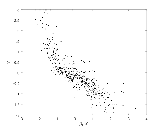
Figure 1: Scatter plot of $Y$ versus the projected covariate $\hat{\beta}_{1}^{\top}X$ in which the direction $\hat{\beta}_{1}$ is obtained by CSE.

The scatter plot of $Y$ against $\hat{\beta}_{1}^{\top}X$ is presented in Figure 1.

$$\rm Figure\ 1\ about\ here$$

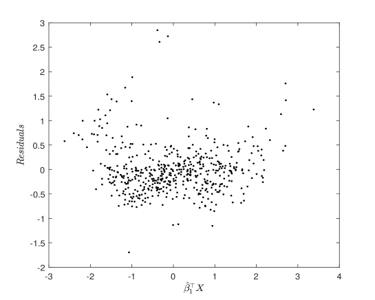
Figure 2: Scatter plot of Residuals from the linear model for $(Y,X)$ versus the projected covariate $\hat{\beta}_{1}$ in which the direction $\hat{\beta}_{1}^{\top}X$ is obtained by CSE.

From this Figure, a linear regression model seems to be plausible to fit the data set. We then apply our test to see whether these exists a model misspecification. The value of the test statistic $AICM_{n}$ is about $0.9639$ and the $p$-value is about $0.01$. Thus a linear regression model is not adequate to predict the response. Figure 2 presents the scatter plot of residuals from the linear regression model for $(Y,X)$ against $\hat{\beta}_{1}^{\top}X$. It also suggests that a linear relationship between $Y$ and $X$ may be not reasonable.

$$\rm Figure\ 2\ about\ here$$

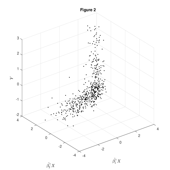
Figure 3: Scatter plot of $Y$ versus the projected predictors $(\hat{\beta}_{1}^{\top}X,\hat{\beta}_{2}^{\top}X)$ in which the directions $(\hat{\beta}_{1},\hat{\beta}_{2})$ are obtained by CSE.

To find the relationship between $Y$ and $X$, we consider a more thorough search of the projected predictor vector. Consider the second projected predictor vector $\hat{\beta}_{2}^{\top}X$ and the scatter plot of $Y$ against $(\hat{\beta}_{1}^{\top}X,\hat{\beta}_{2}^{\top}X)$ is presented in Figure 3.

$$\rm Figure\ 3\ about\ here$$

From this figure, we can see that the second projected direction $\hat{\beta}_{2}^{\top}X$ is not necessary as the plot along this direction is nearly identical. This means the projection of the data onto the space $\hat{\beta}_{1}^{\top}X$ already contain almost all the regression information of the model structure. Furthermore, from Figure 3, it seems that there exists an exponential relationship between $Y$ and $\hat{\beta}_{1}^{\top}X$. Thus we consider $\log(Y)$ as the response variable that is also considered in Harrison and Rubinfeld (1978). Thus we use the following model to fit this data set:

$$\log(Y)=\beta^{\top}X+\varepsilon.$$ (6.1)

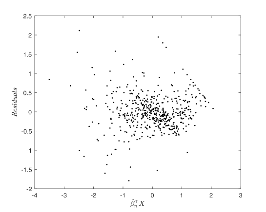
Figure 4: Scatter plot of Residuals from model (5.1) versus the fitted values $\hat{\beta}_{n}^{\top}X$.

When applying our test for the above model (6.1), the value of the test statistic $AICM_{n}$ is about $0.1536$ and the $p$-value is about 0.368. A scatter plot of residuals from model (6.1) against the fitted values is presented in Figure 4. We can see that there does not exist any trend between the residuals and the fitted value. Thus this model is plausible.

$$\rm Figure\ 4\ about\ here$$

7 Discussions

In this article we find that the classic asymptotic results for the ICM test do not hold when the dimension $p$ is divergent. We also show that the wild bootstrap does not valid for the ICM test in the diverging dimension settings. Thus, to overcome this difficult, we construct an adaptive-to-model version of ICM test in terms of sufficient dimension reduction and projection techniques. The proposed test has a non-degenerate limiting null distribution and the wild bootstrap still valid for the new test in the diverging dimension settings. The numerical studies also show that the proposed test largely alleviates the adverse impact of the dimensionality in the sense that it can well maintain the significance level and enhance the power performance. We also show that a large class of weight functions $\varphi(t)$ give the corresponding test statistics with the nice property of computational simplicity. Thus the test can be easily implemented in practice. Furthermore, we obtain the uniformly asymptotically linear presentation of the least squares estimation of the parameters in the nonlinear regression model at a divergent rate $p=o(n^{1/3}/\log{n})$. This result can be useful for further studies in inference. Nevertheless, when the structure dimension $q$ becomes large, the test we proposed here still suffers the same dimensionality problem as in the Bierens’ original ICM test. Thus our new test only partially solves the dimensionality problem. Besides, our test relies on the dimension reduction structure under the null. It is of great interest to investigate goodness of fit testing for hypothetical models without dimension reduction structures in the diverging dimension setting. The relevant studies are ongoing.

Table 1: Empirical sizes and powers of the tests for $H_{11}$ in Study 1.

	a	n=100	n=100	n=100	n=100	n=200	n=400	n=600
		p=2	p=4	p=6	p=8	p=12	p=17	p=20
$AICM_{n},\Sigma_{1}$	0.00	0.0530	0.0510	0.0540	0.0580	0.0540	0.0410	0.0560
	0.25	0.3660	0.3440	0.3560	0.3670	0.6260	0.8710	0.9770
$ACM_{n},\Sigma_{1}$	0.00	0.0600	0.0440	0.0505	0.0440	0.0495	0.0570	0.0510
	0.25	0.2985	0.2645	0.2675	0.2720	0.4960	0.8125	0.9335
$PCVM_{n},\Sigma_{1}$	0.00	0.0540	0.0470	0.0620	0.0660	0.0530	0.0540	0.0650
	0.25	0.3170	0.3020	0.2910	0.3080	0.5140	0.8330	0.9350
$T_{n}^{SZ},\Sigma_{1}$	0.00	0.0500	0.0435	0.0550	0.0475	0.0450	0.0450	0.0450
	0.25	0.2700	0.2880	0.2760	0.2665	0.4945	0.7970	0.9315
$ICM_{n},\Sigma_{1}$	0.00	0.0610	0.0460	0.0200	0.0020	0.0000	0.0000	0.0000
	0.25	0.3220	0.2540	0.1500	0.0200	0.0000	0.0000	0.0000
$T_{n}^{GWZ},\Sigma_{1}$	0.00	0.0505	0.0565	0.0505	0.0345	0.0580	0.0490	0.0605
	0.25	0.2800	0.2650	0.2515	0.2550	0.4435	0.7570	0.9100
$T_{n}^{ZH},\Sigma_{1}$	0.00	0.0395	0.0370	0.0320	0.0305	0.0210	0.0250	0.0285
	0.25	0.1920	0.0855	0.0685	0.0490	0.0370	0.0225	0.0255
$AICM_{n},\Sigma_{2}$	0.00	0.0530	0.0530	0.0460	0.0650	0.0510	0.0460	0.0550
	0.25	0.2950	0.2490	0.2400	0.2250	0.4310	0.6900	0.8570
$ACM_{n},\Sigma_{2}$	0.00	0.0445	0.0395	0.0475	0.0455	0.0500	0.0520	0.0520
	0.25	0.2280	0.1805	0.1745	0.1800	0.2730	0.4935	0.6600
$PCVM_{n},\Sigma_{2}$	0.00	0.0460	0.0600	0.0600	0.0740	0.0630	0.0510	0.0600
	0.25	0.2820	0.2090	0.2030	0.2070	0.2910	0.4940	0.6670
$T_{n}^{SZ},\Sigma_{2}$	0.00	0.0545	0.0405	0.0425	0.0535	0.0555	0.0450	0.0505
	0.25	0.2350	0.2015	0.1805	0.1545	0.2965	0.4905	0.6780
$ICM_{n},\Sigma_{2}$	0.00	0.0490	0.0500	0.0300	0.0030	0.0000	0.0000	0.0000
	0.25	0.2740	0.2130	0.1370	0.0360	0.0000	0.0000	0.0000
$T_{n}^{GWZ},\Sigma_{2}$	0.00	0.0540	0.0595	0.0555	0.0490	0.0525	0.0500	0.0530
	0.25	0.2315	0.1755	0.1680	0.1690	0.2675	0.5045	0.6585
$T_{n}^{ZH},\Sigma_{2}$	0.00	0.0385	0.0360	0.0300	0.0280	0.0305	0.0301	0.0245
	0.25	0.1850	0.0845	0.0560	0.0460	0.0525	0.0390	0.0375

Table 2: Empirical sizes and powers of the tests for $H_{12}$ in Study 1.

	a	n=100	n=100	n=100	n=100	n=200	n=400	n=600
		p=2	p=4	p=6	p=8	p=12	p=17	p=20
$AICM_{n},\Sigma_{1}$	0.00	0.0410	0.0540	0.0550	0.0530	0.0630	0.0550	0.0510
	0.50	0.6570	0.6140	0.6000	0.5830	0.8970	0.9990	1.0000
$ACM_{n},\Sigma_{1}$	0.00	0.0540	0.0510	0.0525	0.0435	0.0595	0.0495	0.0480
	0.50	0.1700	0.1850	0.1780	0.1465	0.3045	0.7255	0.9580
$PCvM_{n},\Sigma_{1}$	0.00	0.0580	0.0590	0.0600	0.0790	0.0470	0.0500	0.0790
	0.50	0.1730	0.1690	0.1460	0.1650	0.2330	0.3860	0.5060
$T_{n}^{SZ},\Sigma_{1}$	0.00	0.0465	0.0570	0.0470	0.0575	0.0475	0.0470	0.0545
	0.50	0.1765	0.1635	0.1925	0.1455	0.3390	0.7415	0.9585
$ICM_{n},\Sigma_{1}$	0.00	0.0540	0.0470	0.0300	0.0010	0.0000	0.0000	0.0000
	0.50	0.4270	0.3380	0.1690	0.0250	0.0000	0.0000	0.0000
$T_{n}^{GWZ},\Sigma_{1}$	0.00	0.0495	0.0510	0.0505	0.0410	0.0440	0.0455	0.0400
	0.50	0.7335	0.6930	0.6420	0.5645	0.9090	0.9965	1.0000
$T_{n}^{ZH},\Sigma_{1}$	0.00	0.0340	0.0430	0.0350	0.0385	0.0325	0.0200	0.0195
	0.50	0.5220	0.2310	0.1180	0.0715	0.0570	0.0420	0.0330
$AICM_{n},\Sigma_{2}$	0.00	0.0540	0.0530	0.0510	0.0560	0.0620	0.0690	0.0510
	0.50	0.6050	0.5260	0.5030	0.4330	0.8000	0.9960	1.0000
$ACM_{n},\Sigma_{2}$	0.00	0.0435	0.0530	0.0550	0.0520	0.0510	0.0490	0.0465
	0.50	0.0860	0.0670	0.0515	0.0500	0.0815	0.1085	0.1545
$PCvM_{n},\Sigma_{2}$	0.00	0.0350	0.0410	0.0600	0.0560	0.0650	0.0480	0.0650
	0.50	0.1050	0.0590	0.0530	0.0700	0.0520	0.0610	0.0510
$T_{n}^{SZ},\Sigma_{2}$	0.00	0.0455	0.0420	0.0455	0.0435	0.0550	0.0465	0.0435
	0.50	0.1035	0.0690	0.0615	0.0600	0.0635	0.1275	0.1770
$ICM_{n},\Sigma_{2}$	0.00	0.0590	0.0440	0.0350	0.0090	0.0000	0.0000	0.0000
	0.50	0.3430	0.2440	0.1250	0.0200	0.0000	0.0000	0.0000
$T_{n}^{GWZ},\Sigma_{2}$	0.00	0.0530	0.0520	0.0515	0.0425	0.0485	0.0655	0.0475
	0.50	0.6800	0.5910	0.5315	0.4785	0.8360	0.9980	1.0000
$T_{n}^{ZH},\Sigma_{2}$	0.00	0.0390	0.0350	0.0345	0.0320	0.0300	0.0280	0.0360
	0.50	0.5550	0.2440	0.1200	0.0795	0.0640	0.0575	0.0495

Table 3: Empirical sizes and powers of the tests for $H_{13}$ in Study 1.

	a	n=100	n=100	n=100	n=100	n=200	n=400	n=600
		p=2	p=4	p=6	p=8	p=12	p=17	p=20
$AICM_{n},\Sigma_{1}$	0.00	0.0550	0.0510	0.0760	0.0510	0.0500	0.0500	0.0650
	0.25	0.5560	0.5640	0.5530	0.5620	0.8530	0.9920	1.0000
$ACM_{n},\Sigma_{1}$	0.00	0.0485	0.0485	0.0560	0.0480	0.0555	0.0440	0.0495
	0.25	0.6275	0.6030	0.6215	0.5830	0.8965	0.9955	1.0000
$PCvM_{n},\Sigma_{1}$	0.00	0.0430	0.0590	0.0540	0.0800	0.0570	0.0650	0.0600
	0.25	0.6040	0.5960	0.6200	0.6090	0.9020	0.9960	1.0000
$T_{n}^{SZ},\Sigma_{1}$	0.00	0.0555	0.0450	0.0455	0.0490	0.0525	0.0590	0.0495
	0.25	0.6335	0.6050	0.6010	0.5820	0.8885	0.9960	1.0000
$ICM_{n},\Sigma_{1}$	0.00	0.0690	0.0540	0.0260	0.0020	0.0000	0.0000	0.0000
	0.25	0.4410	0.3500	0.1600	0.0120	0.0000	0.0000	0.0000
$T_{n}^{GWZ},\Sigma_{1}$	0.00	0.0510	0.0455	0.0495	0.0545	0.0550	0.0510	0.0550
	0.25	0.3920	0.3990	0.4035	0.3735	0.6900	0.9500	0.9960
$T_{n}^{ZH},\Sigma_{1}$	0.00	0.0440	0.0300	0.0390	0.0245	0.0290	0.0235	0.0180
	0.25	0.2240	0.1150	0.0660	0.0525	0.0405	0.0270	0.0255
$AICM_{n},\Sigma_{2}$	0.00	0.0520	0.0430	0.0590	0.0700	0.0570	0.0490	0.0500
	0.25	0.4810	0.8200	0.9160	0.9560	1.0000	1.0000	1.0000
$ACM_{n},\Sigma_{2}$	0.00	0.0505	0.0485	0.0465	0.0455	0.0520	0.0520	0.0520
	0.25	0.6275	0.8845	0.9530	0.9755	1.0000	1.0000	1.0000
$PCvM_{n},\Sigma_{2}$	0.00	0.0480	0.0540	0.0650	0.0670	0.0600	0.0500	0.0570
	0.25	0.5810	0.8720	0.9610	0.9800	1.0000	1.0000	1.0000
$T_{n}^{SZ},\Sigma_{2}$	0.00	0.0490	0.0420	0.0555	0.0550	0.0480	0.0485	0.0495
	0.25	0.6185	0.8775	0.9565	0.9775	1.0000	1.0000	1.0000
$ICM_{n},\Sigma_{2}$	0.00	0.0540	0.0410	0.0340	0.0030	0.0000	0.0000	0.0000
	0.25	0.4510	0.6930	0.6140	0.2630	0.0030	0.0000	0.0000
$T_{n}^{GWZ},\Sigma_{2}$	0.00	0.0470	0.0440	0.0515	0.0460	0.0505	0.0555	0.0480
	0.25	0.3405	0.6680	0.7875	0.8430	0.9980	1.0000	1.0000
$T_{n}^{ZH},\Sigma_{2}$	0.00	0.0455	0.0340	0.0310	0.0355	0.0330	0.0365	0.0365
	0.25	0.2540	0.2990	0.2670	0.1755	0.1965	0.1745	0.1645

Table 4: Empirical sizes and powers of the tests for $H_{14}$ in Study 1.

	a	n=100	n=100	n=100	n=100	n=200	n=400	n=600
		p=2	p=4	p=6	p=8	p=12	p=17	p=20
$AICM_{n},\Sigma_{1}$	0.0	0.0550	0.0540	0.0530	0.0640	0.0520	0.0540	0.0500
	0.1	0.3150	0.3180	0.3090	0.3360	0.5920	0.8630	0.9670
$ACM_{n},\Sigma_{1}$	0.0	0.0525	0.0560	0.0475	0.0505	0.0470	0.0475	0.0575
	0.1	0.3480	0.3320	0.3340	0.3490	0.5900	0.8975	0.9685
$PCvM_{n},\Sigma_{1}$	0.0	0.0440	0.0570	0.0460	0.0470	0.0590	0.0560	0.0530
	0.1	0.3470	0.3570	0.3620	0.3600	0.6510	0.9010	0.9780
$T_{n}^{SZ},\Sigma_{1}$	0.0	0.0510	0.0530	0.0385	0.0515	0.0530	0.0510	0.0530
	0.1	0.3345	0.3440	0.3265	0.3325	0.5830	0.8860	0.9765
$ICM_{n},\Sigma_{1}$	0.0	0.0520	0.0460	0.0210	0.0000	0.0000	0.0000	0.0000
	0.1	0.2580	0.1980	0.1060	0.0170	0.0000	0.0000	0.0000
$T_{n}^{GWZ},\Sigma_{1}$	0.0	0.0520	0.0460	0.0480	0.0465	0.0505	0.0560	0.0515
	0.1	0.2245	0.1930	0.1965	0.1955	0.3720	0.6610	0.8395
$T_{n}^{ZH},\Sigma_{1}$	0.0	0.0410	0.0375	0.0320	0.0280	0.0225	0.0170	0.0200
	0.1	0.1065	0.0645	0.0465	0.0335	0.0285	0.0290	0.0175
$AICM_{n},\Sigma_{2}$	0.0	0.0530	0.0530	0.0510	0.0520	0.0530	0.0630	0.0460
	0.1	0.2870	0.3870	0.4540	0.5370	0.8500	0.9670	0.9710
$ACM_{n},\Sigma_{2}$	0.0	0.0435	0.0395	0.0545	0.0435	0.0435	0.0520	0.0490
	0.1	0.3645	0.4830	0.5930	0.6505	0.9690	0.9995	1.0000
$PCvM_{n},\Sigma_{2}$	0.0	0.0450	0.0570	0.0560	0.0570	0.0560	0.0710	0.0620
	0.1	0.3520	0.4780	0.6080	0.6690	0.9640	1.0000	1.0000
$T_{n}^{SZ},\Sigma_{2}$	0.0	0.0510	0.0550	0.0400	0.0480	0.0465	0.0480	0.0470
	0.1	0.3655	0.5165	0.5935	0.6675	0.9615	0.9995	1.0000
$ICM_{n},\Sigma_{2}$	0.0	0.0630	0.0460	0.0390	0.0050	0.0000	0.0000	0.0000
	0.1	0.2520	0.2720	0.1800	0.0660	0.0001	0.0000	0.0000
$T_{n}^{GWZ},\Sigma_{2}$	0.0	0.0435	0.0505	0.0455	0.0435	0.0515	0.0455	0.0590
	0.1	0.1950	0.2265	0.3230	0.3225	0.7000	0.9765	0.9985
$T_{n}^{ZH},\Sigma_{2}$	0.0	0.0295	0.0315	0.0335	0.0310	0.0320	0.0270	0.0320
	0.1	0.1240	0.0990	0.0990	0.0945	0.1080	0.0900	0.0885

Table 5: Empirical sizes and powers of the tests $AICM_{n},PCvM_{n},ICM_{n},$ and $T_{n}^{ZH}$ for $H_{21}$ in Study 2.

	a	n=100	n=100	n=100	n=100	n=200	n=400	n=600
		p=2	p=4	p=6	p=8	p=12	p=17	p=20
$AICM_{n},\Sigma_{1}$	0.0	0.0610	0.0690	0.0720	0.0650	0.0640	0.0580	0.0650
	0.5	0.5040	0.4130	0.3230	0.2850	0.6390	0.9780	1.0000
$PCvM_{n},\Sigma_{1}$	0.0	0.0540	0.0550	0.0650	0.0680	0.0750	0.0680	0.0760
	0.5	0.4540	0.3910	0.3270	0.2390	0.5030	0.8620	0.9820
$ICM_{n},\Sigma_{1}$	0.0	0.0470	0.0610	0.0280	0.0170	0.0000	0.0000	0.0000
	0.5	0.4270	0.2920	0.1460	0.0460	0.0000	0.0000	0.0000
$T_{n}^{ZH},\Sigma_{1}$	0.0	0.0280	0.0255	0.0250	0.0215	0.0220	0.0270	0.0170
	0.5	0.3285	0.1210	0.0615	0.0405	0.0335	0.0325	0.0345
$AICM_{n},\Sigma_{2}$	0.0	0.0610	0.0670	0.0540	0.0820	0.0850	0.0670	0.0560
	0.5	0.4950	0.8120	0.8820	0.9020	1.0000	1.0000	1.0000
$PCvM_{n},\Sigma_{2}$	0.0	0.0470	0.0700	0.0630	0.0740	0.0790	0.0670	0.0600
	0.5	0.4780	0.7130	0.7570	0.7400	0.9930	1.0000	0.9990
$ICM_{n},\Sigma_{2}$	0.0	0.0510	0.0700	0.0450	0.0250	0.0000	0.0000	0.0000
	0.5	0.4690	0.7310	0.7520	0.5070	0.2870	0.0050	0.0050
$T_{n}^{ZH},\Sigma_{2}$	0.0	0.0340	0.0265	0.0210	0.0315	0.0320	0.0240	0.0355
	0.5	0.3465	0.4445	0.3470	0.2405	0.3135	0.2835	0.2760

Table 6: Empirical sizes and powers of the tests $AICM_{n},PCvM_{n},ICM_{n},$ and $T_{n}^{ZH}$ for $H_{22}$ in Study 2.

	a	n=100	n=100	n=100	n=100	n=200	n=400	n=600
		p=2	p=4	p=6	p=8	p=12	p=17	p=20
$AICM_{n},\Sigma_{1}$	0.0	0.0580	0.0570	0.0700	0.0700	0.0790	0.0560	0.0720
	0.5	0.5670	0.5160	0.4890	0.4030	0.7780	0.9880	1.0000
$PCvM_{n},\Sigma_{1}$	0.0	0.0640	0.0680	0.0660	0.0880	0.0770	0.0610	0.0500
	0.5	0.3840	0.3600	0.3440	0.3080	0.5420	0.8100	0.9110
$ICM_{n},\Sigma_{1}$	0.0	0.0530	0.0530	0.0360	0.0170	0.0000	0.0000	0.0000
	0.5	0.5290	0.4550	0.3210	0.0880	0.0000	0.0000	0.0000
$T_{n}^{ZH},\Sigma_{1}$	0.0	0.0315	0.0350	0.0240	0.0230	0.0230	0.0240	0.0220
	0.5	0.4905	0.1815	0.0910	0.0565	0.0500	0.0525	0.0335
$AICM_{n},\Sigma_{2}$	0.0	0.0570	0.0520	0.0760	0.0850	0.0690	0.0680	0.0670
	0.5	0.5840	0.4380	0.3750	0.3810	0.7010	0.9700	1.0000
$PCvM_{n},\Sigma_{2}$	0.0	0.0690	0.0590	0.0780	0.0830	0.0680	0.0610	0.0550
	0.5	0.3870	0.1630	0.1030	0.0930	0.0740	0.0730	0.0530
$ICM_{n},\Sigma_{2}$	0.0	0.0640	0.0700	0.0450	0.0210	0.0000	0.0000	0.0000
	0.5	0.5470	0.3390	0.1720	0.0840	0.0010	0.0000	0.0000
$T_{n}^{ZH},\Sigma_{2}$	0.0	0.0305	0.0265	0.0270	0.0230	0.0190	0.0295	0.0275
	0.5	0.5160	0.2200	0.0950	0.0625	0.0545	0.0550	0.0430

Table 7: Empirical sizes and powers of the tests $AICM_{n},PCvM_{n},ICM_{n},$ and $T_{n}^{ZH}$ for $H_{23}$ in Study 2.

	a	n=100	n=100	n=100	n=100	n=200	n=400	n=600
		p=2	p=4	p=6	p=8	p=12	p=17	p=20
$AICM_{n},\Sigma_{1}$	0.00	0.0590	0.0710	0.0610	0.0790	0.0740	0.0700	0.0610
	0.75	0.2270	0.2620	0.2660	0.3060	0.5250	0.8390	0.9680
$PCvM_{n},\Sigma_{1}$	0.00	0.0480	0.0630	0.0610	0.0690	0.0730	0.0600	0.0630
	0.75	0.1020	0.1530	0.1670	0.2170	0.2820	0.3320	0.3730
$ICM_{n},\Sigma_{1}$	0.00	0.0520	0.0670	0.0400	0.0090	0.0000	0.0000	0.0000
	0.75	0.1990	0.1620	0.0840	0.0230	0.0000	0.0000	0.0000
$T_{n}^{ZH},\Sigma_{1}$	0.00	0.0320	0.0280	0.0230	0.0270	0.0270	0.0225	0.0225
	0.75	0.1940	0.0705	0.0525	0.0380	0.0365	0.0375	0.0280
$AICM_{n},\Sigma_{2}$	0.00	0.0390	0.0740	0.0730	0.0760	0.0750	0.0690	0.0600
	0.75	0.4440	0.7200	0.8100	0.7720	0.9940	0.9970	1.0000
$PCvM_{n},\Sigma_{2}$	0.00	0.0480	0.0700	0.0610	0.0680	0.0780	0.0580	0.0570
	0.75	0.2330	0.2160	0.1750	0.1330	0.1270	0.1510	0.1440
$ICM_{n},\Sigma_{2}$	0.00	0.0580	0.0650	0.0540	0.0220	0.0000	0.0000	0.0000
	0.75	0.3760	0.6500	0.6020	0.3500	0.0690	0.0010	0.0000
$T_{n}^{ZH},\Sigma_{2}$	0.00	0.0300	0.0240	0.0315	0.0240	0.0245	0.0325	0.0330
	0.75	0.3860	0.3795	0.2925	0.1950	0.2220	0.1970	0.2050

Table 8: Empirical sizes and powers of the tests for $H_{31}$ in Study 3.

	a	n=50	n=100	n=200	n=500	n=1000
		p=5	p=10	p=20	p=50	p=100
$AICM_{n},\Sigma_{1}$	0.0	0.0620	0.0570	0.0640	0.0710	0.0810
	0.1	0.1630	0.2500	0.4480	0.8580	0.9940
$ACM_{n},\Sigma_{1}$	0.0	0.0395	0.0475	0.0465	0.0580	0.0575
	0.1	0.2015	0.3615	0.6380	0.9550	1.0000
$PCvM_{n},\Sigma_{1}$	0.0	0.0510	0.0710	0.0710	0.0750	0.0810
	0.1	0.1970	0.3620	0.6520	0.9420	1.0000
$T_{n}^{SZ},\Sigma_{1}$	0.0	0.0500	0.0560	0.0555	0.0560	0.0420
	0.1	0.1975	0.3560	0.6425	0.9615	0.9990
$ICM_{n},\Sigma_{1}$	0.0	0.0200	0.0000	0.0000	0.0050	0.9940
	0.1	0.0810	0.0010	0.0000	0.0090	0.9720
$T_{n}^{GWZ},\Sigma_{1}$	0.0	0.0450	0.0535	0.0445	0.0660	0.0850
	0.1	0.2315	0.5400	0.9075	1.0000	0.9100
$T_{n}^{ZH},\Sigma_{1}$	0.0	0.0295	0.0240	0.0145	0.0275	0.0000
	0.1	0.0400	0.0340	0.0170	0.0210	0.0000
$AICM_{n},\Sigma_{2}$	0.0	0.0640	0.0680	0.0750	0.0790	0.1070
	0.1	0.2350	0.5820	0.8490	0.9350	0.9590
$ACM_{n},\Sigma_{2}$	0.0	0.0500	0.0485	0.0455	0.0470	0.0550
	0.1	0.4535	0.8795	0.9965	1.0000	1.0000
$PCvM_{n},\Sigma_{2}$	0.0	0.0600	0.0520	0.0590	0.0650	0.0610
	0.1	0.4210	0.8180	0.9870	0.9990	1.0000
$T_{n}^{SZ},\Sigma_{2}$	0.0	0.0595	0.0440	0.0520	0.0490	0.0550
	0.1	0.4900	0.9110	0.9985	1.0000	1.0000
$ICM_{n},\Sigma_{2}$	0.0	0.0370	0.0000	0.0000	0.0040	0.9890
	0.1	0.1450	0.0020	0.0000	0.0000	0.0030
$T_{n}^{GWZ},\Sigma_{2}$	0.0	0.0475	0.0540	0.0515	0.0630	0.0925
	0.1	0.2360	0.5315	0.9055	1.0000	1.0000
$T_{n}^{ZH},\Sigma_{2}$	0.0	0.0275	0.0295	0.0240	0.3200	0.0000
	0.1	0.1210	0.0990	0.0540	0.3170	0.0000

Table 9: Empirical sizes and powers of the tests for $H_{32}$ in Study 3.

	a	n=50	n=100	n=200	n=500	n=1000
		p=5	p=10	p=20	p=50	p=100
$AICM_{n},\Sigma_{1}$	0.0	0.0870	0.0780	0.1000	0.1390	0.1700
	0.5	0.8000	0.9690	0.9960	1.0000	1.0000
$PCvM_{n},\Sigma_{1}$	0.0	0.0900	0.0760	0.1060	0.1250	0.1650
	0.5	0.8080	0.9680	0.9950	0.9990	1.0000
$ICM_{n},\Sigma_{1}$	0.0	0.0410	0.0050	0.1410	0.9970	0.9970
	0.5	0.5620	0.1680	0.1610	0.8410	0.8900
$T_{n}^{ZH},\Sigma_{1}$	0.0	0.0170	0.0180	0.0105	0.0240	0.0000
	0.5	0.1945	0.0915	0.0250	0.0270	0.0000
$AICM_{n},\Sigma_{2}$	0.0	0.0750	0.0960	0.1070	0.1060	0.1270
	0.5	0.7480	0.7440	0.7910	0.8020	0.8640
$PCvM_{n},\Sigma_{2}$	0.0	0.0930	0.0830	0.0770	0.0670	0.0840
	0.5	0.7030	0.8010	0.7880	0.7800	0.8450
$ICM_{n},\Sigma_{2}$	0.0	0.0660	0.0130	0.0540	0.8940	0.8970
	0.5	0.6310	0.1200	0.0000	0.0000	0.0030
$T_{n}^{ZH},\Sigma_{2}$	0.0	0.0175	0.0255	0.0205	0.3145	0.0000
	0.5	0.6790	0.6085	0.1700	0.3585	0.0000