Microscopic three-cluster study of light exotic nuclei

Abstract

I develop a microscopic three-cluster model for exotic light nuclei. I use the hyperspherical formalism, associated with the Generator Coordinate Method. This model is well adapted to halo nuclei, since the long-range part of the radial wave functions is accurately reproduced. The core wave functions are described in the shell model, including excited states. This technique provides large bases, expressed in terms of projected Slater determinants. Matrix elements involve seven-dimension integrals, and therefore require long calculation times. I apply the model to ¹¹Li, ¹⁴Be, ¹⁵B, and ¹⁷N described by two neutrons surrounding a ⁹Li, ¹²Be, ¹³B and ¹⁵N core, respectively. The ¹⁷Ne (as ¹⁵O+p+p) and ¹⁵Ne (as ¹³O+p+p) mirror nuclei are briefly discussed. I present the spectra and some spectroscopic properties, such as r.m.s. radii or E2 transition probabilities. I also analyze the importance of core excitations.

I Introduction

Exotic nuclei represent one of the major interests in modern nuclear physics Tanihata et al. (2013). These nuclei are located close to the driplines (neutron or proton) and, owing to the low binding energy, present specific properties, such as an anomalously large radius or modifications of the shell structure. Recent development of experimental facilities have provided a large number of new data, which need to be understood by theory.

The main property of exotic nuclei being their low binding energy, the relative wave functions extend to large distances. Theoretical models therefore need to reproduce this property. A widely used approach is the hyperspherical method Lin (1995), where the Jacobi coordinates are replaced by a set of angles, and by a single length, referred to as the hyperradius. The three-body equation is then replaced by a set of coupled differential equations depending on the hyperradius. The hyperspherical formalism can be extended to systems involving more than three particles Gattobigio et al. (2011). Many works in atomic and in nuclear physics have been performed within this method.

In nuclear physics, most applications are carried out in non-microscopic models. In other words, the nucleus is seen as a three-body system, with a structureless core, and two external nucleons. Typical applications are the ⁶He and ¹¹Li nuclei, modeled by $\alpha$+n+n and ⁹Li+n+n three-body structures. This approach therefore relies on nucleon+nucleon and nucleon+core potentials. It simulates the Pauli principle by an appropriate choice of these interactions. Core excitations are in general neglected.

This non-microscopic model can be extended to microscopic theories, where the system is described by a $A$-body Hamiltonian. The core nucleus is defined in the shell model, and a full antisymmetrization is taken into account. The use of the hyperspherical formalism guarantees the correct long-range behaviour of the wave function. The model only relies on a nucleon-nucleon interaction, and on the description of the core wave functions. In contrast with non-microscopic models, it allows to include core excitations without any further parameter.

Microscopic cluster models are used in nuclear physics for many years (see reviews in Refs. Descouvemont and Dufour (2012); Horiuchi et al. (2012)) but most applications deal with the two-cluster variant, much easier than multicluster approaches. The application of the hyperspherical formalism to microscopic cluster theories is recent. The first works were focused on ⁶He Filippov et al. (1996); Korennov and Descouvemont (2004) which involves the $\alpha$ particle as a core. The $\alpha$ particle can be accurately described by a $(0s)^{4}$ shell model configuration which makes the calculations relatively easy. The model was extended to three-body continuum states Damman and Descouvemont (2009), and microscopic ⁶He wave functions have been used in CDCC calculations of elastic scattering on heavy targets Descouvemont (2016).

The main limitation of microscopic three-cluster models in hyperspherical coordinates is that the matrix elements involve the numerical calculation of (many) seven-dimension integrals Korennov and Descouvemont (2004). Consequently, applications are essentially limited to light systems, most of them involving an $\alpha$ core. In addition to the ⁶He system mentioned above, a recent application focuses on ⁸Li, described by an $\alpha+^{3}$H+n three-cluster configuration Descouvemont and Pinilla (2019).

The aim of the present work is to go beyond this limitation. The development of the computing technology, and in particular of the parallelization possibilities permits to consider heavier systems, involving $p$-shell nuclei as the core. I analyze four nuclei (¹¹Li, ¹⁴Be, ¹⁵B, ¹⁷N) which are modelled by a $p$-shell core and two surrounding neutrons. Compared to previous applications, the present calculations face two difficulties: (1) the presence of $p$-shell orbitals, and (2) the need of several Slater determinants for the core.

The paper is organized as follows. In Sec. II, I present a general overview of the microscopic three-cluster model. In Sec. III, I apply the method to various exotic nuclei. Concluding remarks are presented in Sec. IV.

II Microscopic three-cluster model in hyperspherical coordinates

II.1 General overview

My main goal is to solve a $A$-body problem, where the Hamiltonian is given by

$$H=\sum_{i=1}^{A}t_{i}+\sum_{i<j=1}^{A}v_{ij}.$$ (1)

In this definition, $t_{i}$ is the kinetic energy of nucleon $i$, and $v_{ij}$ a nucleon-nucleon interaction which contains nuclear and Coulomb components. Recent ab initio models (see, for example, Ref. Blumenfeld et al. (2013)) are developed to find exact solutions of the Schrödinger equation associated with (1). These models, however, are in general not well adapted to halo nuclei, where the long-range part of the wave functions plays a crucial role. My approach, in contrast, is based on the cluster approximation Wildermuth and Tang (1977); Descouvemont and Dufour (2012).

The total wave function, solution of the Schrödinger equation

$$(H-E)\Psi=0,$$ (2)

is written schematically as

$$\Psi={\cal A}\phi_{1}\phi_{2}\phi_{3}G,$$ (3)

where $\phi_{i}$ are the internal wave functions of the clusters (in practice, they are defined in the shell model), and $G$ is a radial function, depending on the relative coordinates between the clusters. The antisymmetrization operator ${\cal A}$ ensures that the wave function is completely antisymmetric.

The cluster approximation permits a strong simplification of the calculations, in comparison with ab initio models. It is also well adapted to halo nuclei or, more generally, to states presenting a strong cluster structure. Owing to this approximation, however, effective nucleon-nucleon interactions $v_{ij}$, such as the Volkov Volkov (1965) or the Minnesota Thompson et al. (1977) force, must be used. These forces simulate missing effects, such as the tensor component, by an effective central interaction. Ideally, three-body forces should be introduced, and developments have been achieved in that direction for realistic forces (see Ref. Machleidt et al. (2013) for a review). For effective interactions, however, even if some work has been done Kanada-En’yo and Akaishi (2004); Itagaki (2016), the use of three-body forces is essentially limited to well bound nuclei, such as ¹²C or ¹⁶O. In most cluster calculations, three-body forces are therefore neglected.

Several variants of microscopic cluster models exist. Of course, the simplest version is a two-cluster model, which is used since many years Horiuchi (1977). Three-cluster models have been developed in various directions: frozen triangular configurations Descouvemont (1995), 2+1 configurations essentially aimed for nucleus-nucleus scattering such as ⁷Be+p Descouvemont (2004), and, more recently, genuine three-body models using the hyperspherical formalism Korennov and Descouvemont (2004). The present work is based on the hyperspherical approach, which is described in more detail in the next subsections.

II.2 Core wave functions

Let me consider Eq. (3) where the internal wave functions $\phi_{i}$ are associated with three clusters with nucleon numbers ($A_{1},A_{2},A_{3}$) and charge numbers ($Z_{1},Z_{2},Z_{3}$). I assume that clusters 2 and 3 are $s$-shell nuclei and, more specifically in the present work, that they are neutrons. I also assume that the oscillator parameter $b$ is common to the three clusters. Until now, the use of the hyperspherical formalism in microscopic models was limited to an $\alpha$ core. This is well adapted, for example, to ⁶HeKorennov and Descouvemont (2004), ⁶Li Korennov and Descouvemont (2004), or ⁸B Descouvemont and Pinilla (2019). The main reason for this limitation is that, as it will be discussed later, matrix elements involve seven-dimensional integrals.

This limitation, however, restricts the applications to a few light nuclei. In the present work, I go beyond this limitation, and extends the model to $p$-wave orbitals. The consequences in terms of computer times are twofold: ($i$) the matrix elements involve $p$-shell orbitals which has a strong impact on the matrix elements of the nucleon-nucleon interaction (quadruple sums over the individual orbitals); ($ii$) $p$-shell nuclei such as ⁹Li or ¹²Be involve several Slater determinants (up to 90 for ⁹Li), whereas the $\alpha$ particle is described by a single Slater determinant.

I remind here the main properties. Let me consider a Slater determinant $\bar{\Phi}_{i}$ involving $A_{1}$ single-particle orbitals

$$\varphi_{n_{x}n_{y}n_{z}m_{s}m_{t}}(\boldsymbol{r})=$$

$$\hskip 28.45274pt\varphi_{n_{x}}(x)\varphi_{n_{y}}(y)\varphi_{n_{z}}(z)|\frac{1}{2}m_{s}\rangle|\frac{1}{2}m_{t}\rangle,$$ (4)

where $\varphi_{n}(s)$ are harmonic oscillator functions and where $m_{s},m_{t}=\pm 1/2$ are associated with the spin and the isospin, respectively. The first step is to define the list of $N_{S}$ Slater determinants consistent with the Pauli principle. Assuming that the $s$-shell is filled, the number of Slater determinants for $p$-shell nuclei is $N_{S}=C_{6}^{Z_{1}-2}\times C_{6}^{N_{1}-2}$, where $C_{i}^{j}$ is the number of combinations of $j$ elements among $i$ elements. For ⁹Li, ¹²Be, ¹³B and ¹⁵N, I have $N_{S}=90,15,20,6$, respectively. The $N_{S}$ Slater determinants $\bar{\Phi}_{i}$ must be projected on the various angular momenta $I,L,S,T$ from a diagonalization of the $\boldsymbol{I}^{2},\boldsymbol{L}^{2},\boldsymbol{S}^{2}$ and $\boldsymbol{T}^{2}$ operators ($\boldsymbol{I}=\boldsymbol{L}+\boldsymbol{S}$). This procedure provides basis functions with good quantum numbers as

$$\Phi^{I\nu}_{1,LST}=\sum_{i=1}^{N_{S}}d^{I\nu LST}_{i}\,\bar{\Phi}_{i}.$$ (5)

Finally, basis functions (5) are used to diagonalize the Hamiltonian (1) for cluster 1, and I get the core wave functions as

$$\Phi^{I\nu}_{1}=\sum_{LST}D^{I\nu}_{LST}\Phi^{I\nu}_{1,LST}.$$ (6)

This technique corresponds to a standard shell-model approach, and can be extended to higher shells (the summation may involve an additional quantum number, associated with the degeneracy). The specificity of the cluster model is that (6) is only the very first step of the calculations. These internal wave functions must then be introduced in the three-body wave functions (3).

II.3 Three-cluster wave functions

Let me come back to the three-cluster wave functions (3). In the Generator Coordinate Method (GCM, see Refs. Horiuchi (1977); Descouvemont and Dufour (2012)), the clusters are located at three points, as represented in Fig. 1. The generator coordinates $\boldsymbol{R}_{1}$ is associated with the external clusters (neutrons in the present applications) and $\boldsymbol{R}_{2}$ with the relative motion between the core and the c.m. of clusters 2 and 3. They are variational parameters, and are not associated with the nucleon coordinates (in other words, the antisymmetrization operator does not act on $\boldsymbol{R}_{1}$ and $\boldsymbol{R}_{2}$). A GCM basis state is defined as

$$\Phi^{\nu_{1}\nu_{2}\nu_{3}}_{c_{1}}(\boldsymbol{R}_{1},\boldsymbol{R}_{2})={\cal A}\Phi^{\nu_{1}}_{c_{1}}\bigl{(}-\frac{A_{23}}{A}\boldsymbol{R}_{2}\bigr{)}$$

$$\hskip 14.22636pt\times\Phi^{\nu_{2}}_{2}\bigl{(}\frac{A_{23}}{A}\boldsymbol{R}_{2}+\frac{A_{1}}{A_{12}}\boldsymbol{R}_{1}\bigr{)}\Phi^{\nu_{3}}_{3}\bigl{(}\frac{A_{23}}{A}\boldsymbol{R}_{2}-\frac{A_{1}}{A_{12}}\boldsymbol{R}_{1}\bigr{)},$$ (7)

where $\Phi^{\nu_{1}}_{c_{1}}$ are the core wave functions (6), and $\Phi^{\nu_{2}}_{2}$ and where $\Phi^{\nu_{3}}_{3}$ correspond to the external clusters. In this equation, $A_{12}=A_{1}+A_{2}$ and $A_{23}=A_{2}+A_{3}$. If the internal wave functions are defined in the harmonic oscillator model with a common oscillator parameter $b$, these basis functions are Slater determinants, and the c.m. motion is factorized exactly. For the sake of clarity, I do not write the spins $I_{i}$ of the clusters.

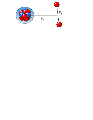
Figure 1: Three-cluster configuration using the generator coordinates $\boldsymbol{R}_{1}$ and $\boldsymbol{R}_{2}$ [see Eq. (7)].

A first angular-momentum coupling is performed on the spins $I_{2}$ and $I_{3}$ of the external clusters with

$$\Phi^{I_{23}I\nu}_{c_{1}}(\boldsymbol{R}_{1},\boldsymbol{R}_{2})=\sum_{\nu_{1}\nu_{2}\nu_{3}}\langle I_{2}\,\nu_{2}\,I_{3}\,\nu_{3}|I_{23}\,\nu_{2}+\nu_{3}\rangle$$

$$\times\langle I_{1}\,\nu_{1}I_{23}\,\nu_{2}+\nu_{3}|I\,\nu\rangle\Phi^{\nu_{1}\nu_{2}\nu_{3}}_{c_{1}}(\boldsymbol{R}_{1},\boldsymbol{R}_{2}).$$ (8)

Then I introduce the hyperspherical formalism, well known in non-microscopic models Zhukov et al. (1993), and extended more recently to microscopic theories Korennov and Descouvemont (2004); Kievsky et al. (2008). I define scaled Jacobi coordinates as

$$\boldsymbol{X}=\sqrt{\frac{A_{2}A_{3}}{A_{23}}}\boldsymbol{R}_{1},$$

$$\boldsymbol{Y}=\sqrt{\frac{A_{1}A_{23}}{A}}\boldsymbol{R}_{2},$$ (9)

which provide the hyperradius $R$ and hyperangle $\alpha$ from

$$R=\sqrt{\boldsymbol{X}^{2}+\boldsymbol{Y}^{2}},$$

$$\tan\alpha=Y/X.$$ (10)

Both coordinates are complemented by the angles associated with $\boldsymbol{X}$ and $\boldsymbol{Y}$ as

$$\Omega_{5}=(\alpha,\Omega_{X},\Omega_{Y}).$$ (11)

From the basis functions (8), I project on the total angular momentum $J$ and parity $\pi$. This is achieved by a double projection on the orbital momenta $\ell_{x}$ and $\ell_{y}$; a projected basis function is written as

$$\tilde{\Phi}^{JM\pi}_{c_{1}I_{23}I\ell_{x}\ell_{y}L}(R_{1},R_{2})=\sum_{\nu M_{L}}\langle I\nu LM_{L}|JM\rangle$$

$$\hskip 5.69046pt\times\int d\Omega_{X}d\Omega_{Y}\bigl{[}Y_{\ell_{x}}^{\ast}(\Omega_{X})\otimes Y_{\ell_{y}}^{\ast}(\Omega_{Y})\bigr{]}^{LM_{L}}\Phi^{I_{23}I\nu}_{c_{1}}(\boldsymbol{R}_{1},\boldsymbol{R}_{2}),$$ (12)

which represents a four-dimension integral. This double-projection technique has been used in three-body models aimed at studying nucleus-nucleus scattering such as ⁷Be+p Descouvemont and Baye (1994) for example. In the hyperspherical formalism, one introduces the hypermoment $K$, which is a generalization of the angular momentum in three-body systems. An hyperspherical basis function reads

$$\Phi^{JM\pi}_{\gamma K}(R)= \int d\alpha\cos^{2}\alpha\sin^{2}\alpha\,\varphi_{K}^{\ell_{x}\ell_{y}}(\alpha)$$

$$\times\tilde{\Phi}^{JM\pi}_{\gamma}(R\sin\alpha,R\cos\alpha),$$ (13)

where index $\gamma$ stands for $\gamma=(c_{1}I_{23}I\ell_{x}\ell_{y}L)$. In this equation, function $\varphi_{K}^{\ell_{x}\ell_{y}}(\alpha)$ is defined by

$$\varphi_{K}^{\ell_{x}\ell_{y}}(\alpha)= {\cal N}_{K}^{\ell_{x}\ell_{y}}(\cos\alpha_{R})^{\ell_{y}}(\sin\alpha_{R})^{\ell_{x}}$$

$$\times P_{n}^{\ell_{y}+1/2,\ell_{x}+1/2}(\cos 2\alpha),$$ (14)

$P_{n}^{a,b}(x)$ being a Jacobi polynomial. The normalization coefficient ${\cal N}_{K}^{\ell_{x}\ell_{y}}$ is given by

$${\cal N}_{K}^{\ell_{x}\ell_{y}}=\bigg{[}\frac{2n!(K+2)(n+\ell_{x}+\ell_{y}+1)!}{\Gamma(n+\ell_{x}+\frac{3}{2})\Gamma(n+\ell_{y}+\frac{3}{2})}\bigg{]}^{\frac{1}{2}},$$ (15)

where $n=(K-\ell_{x}-\ell_{y})/2$ is a positive integer. The main advantage of the hyperspherical formalism is to reduce the number of degrees of freedom to one. The configuration space is therefore spanned by a single generator coordinate $R$. This approach is also well adapted to three-body continuum states Damman and Descouvemont (2009). Of course, matrix elements between basis states (13) are more demanding in terms of computer times, since they involve seven-dimensional integrals (see next subsection) which must be performed numerically.

The total wave function of the system is given by a superposition of basis functions (13) as

$$\Psi^{JM\pi}=\sum_{\gamma K}\sum_{i=1}^{N}f^{J\pi}_{\gamma Ki}\,\Phi^{JM\pi}_{\gamma K}(R_{i}),$$ (16)

where $N$ is the number of generator coordinates (typically $N\approx 10$). In this expansion, the summation over the hypermoment $K$ is limited to a maximum value $K_{\rm max}$. As usual in hyperspherical models, $K_{\rm max}$ must be large enough to ensure the convergence of the physical quantities (energies, radii, etc.). Coefficients $f^{J\pi}_{\gamma Ki}$ represent the generator function, and are obtained from a diagonalization of the Hamiltonian kernel.

II.4 Matrix elements

The main part of the calculation concerns matrix elements between projected basis functions (13). The Hamiltonian kernel reads

$$H^{J\pi}_{\gamma K,\gamma^{\prime}K^{\prime}}(R,R^{\prime})=\langle\Phi^{J\pi}_{\gamma K}(R)|H|\Phi^{J\pi}_{\gamma^{\prime}K^{\prime}}(R^{\prime})\rangle$$

$$=\int\cos^{2}\alpha\sin^{2}\alpha\cos^{2}\alpha^{\prime}\sin^{2}\alpha^{\prime}\,\varphi_{K}^{\ell_{x}\ell_{y}}(\alpha)\,\varphi_{K^{\prime}}^{\ell_{x}^{\prime}\ell_{y}^{\prime}}(\alpha^{\prime})$$

$$\times\tilde{H}^{J}_{\gamma,\gamma^{\prime}}(R\sin\alpha,R\cos\alpha;R^{\prime}\sin\alpha^{\prime},R^{\prime}\cos\alpha^{\prime})d\alpha\,d\alpha^{\prime},$$ (17)

where

$$\tilde{H}^{J\pi}_{\gamma,\gamma^{\prime}}(R_{1},R_{2};R^{\prime}_{1},R^{\prime}_{2})=\langle\tilde{\Phi}^{J\pi}_{\gamma}(R_{1},R_{2})|H|\tilde{\Phi}^{J\pi}_{\gamma^{\prime}}(R^{\prime}_{1},R^{\prime}_{2})\rangle,$$ (18)

with $\tilde{\Phi}^{J\pi}_{\gamma}(R_{1},R_{2})$ given by Eq. (12). The projection over the hypermoment therefore represents a double integration over $\alpha$ and $\alpha^{\prime}$. This quadrature is performed numerically. From Eq. (12), the matrix elements (18) involve eight angular integrals. In fact, owing to the rotation invariance, three angles can be fixed, which leads to five-dimensional integrals. The calculation provides

$$\langle\tilde{\Phi}^{J\pi}_{\gamma}(R_{1},R_{2})|H|\tilde{\Phi}^{J\pi}_{\gamma^{\prime}}(R^{\prime}_{1},R^{\prime}_{2})\rangle=\frac{8\pi^{2}}{2J+1}\sum_{M_{L},M^{\prime}_{L},\nu,\nu^{\prime}}\langle I\,\nu\,L\,M_{L}|J\,\nu+M_{L}\rangle\langle I^{\prime}\,\nu^{\prime}\,L^{\prime}\,M^{\prime}_{L}|J\,\nu^{\prime}+M^{\prime}_{L}\rangle$$

$$\times\int\bigl{[}Y^{\ast}_{\ell_{x}}(\Omega_{X^{\prime}})\otimes Y^{\ast}_{\ell_{y}}(0,0)\bigr{]}^{LM_{L}}\bigl{[}Y_{\ell_{x^{\prime}}}(\Omega_{X^{\prime}})\otimes Y_{\ell_{y^{\prime}}}(\theta_{Y^{\prime}},0)\bigr{]}^{L^{\prime}M^{\prime}_{L}}$$

$$\times\langle\Phi_{c_{1}}^{I_{23}I\nu}(\boldsymbol{R}_{1},\boldsymbol{R}_{2})|H|\Phi_{c^{\prime}_{1}}^{I^{\prime}_{23}I^{\prime}\nu^{\prime}}(\boldsymbol{R}^{\prime}_{1},\boldsymbol{R}^{\prime}_{2})\rangle\,d\Omega_{X}d\Omega_{X^{\prime}}\sin\theta_{Y^{\prime}}d\theta_{Y^{\prime}},$$ (19)

where $\boldsymbol{R}_{2}$ is along the $z$ axis and $\boldsymbol{R}^{\prime}_{2}$ is in the $xz$ plane. This expression is also valid for other rotation-invariant operators. A generalization to operators, such as the electromagnetic operators, is straightforward.

The calculation of the matrix elements (18) is therefore performed in several steps:

1. Matrix elements between Slater determinants ${\cal A}\bar{\Phi}_{i}\Phi^{\nu_{2}}_{2}\Phi^{\nu_{3}}_{3}$ are first computed. One-body operators involve double sums over the individual orbitals, whereas two-body operators involve quadruple sums. When dealing with three $s$ clusters, the quadruple sums contain $3^{4}$ terms, but this amounts to $6^{4}$ when one cluster belongs to the $p$ shell. Compared to previous works on ⁶He or ¹²C this property makes the calculations 16 times longer.

2. Matrix elements between wave functions (7) are then constructed with the transformation coefficients (6). The number of three-cluster Slater determinants is given by $N_{S}(2I_{2}+1)(2I_{3}+1)$. For ⁶He, this number is 4, since the core is an $\alpha$ particle. For ¹¹Li, in contrast, the core involves 90 functions, and the total number of Slater determinants (7) is therefore 360.

3. The next step is to compute the projected matrix elements (19) which involve five numerical quadratures (typically $\sim 16-20$ points are used for each angle).

4. Finally the projection over the hypermomentum is performed with (17). For a given set of generator coordinates $(R,R^{\prime})$, all integrals are evaluated simultaneously.

This process must be repeated for all sets of $(R,R^{\prime})$ values. For systems such as ¹¹Li which involve many Slater determinants, the full calculation is extremely time consuming. This can be achieved with an optimization of the codes, and using modern computing facilities. In practice, a parallelization is performed over the hyperangles $\alpha$ and $\alpha^{\prime}$ in (17). Let me also mention that the total number of basis functions (i.e. the size of the matrices) can be as large as 20000. This raises precision issues since the basis is (highly) non orthogonal.

III Application to light exotic nuclei

III.1 Conditions of the calculations

The calculations are performed with the Volkov V2 nucleon-nucleon interaction Volkov (1965). For the oscillator parameter, I use $b=1.60$ fm, a standard value for $p$-shell nuclei. The optimal $b$ value stems from a compromise: to reproduce the core radius, and to minimize the binding energy of the core. Small variations of $b$ can be compensated by a slight readjustment of the nucleon-nucleon interaction. The first step is to determine the core wave functions (6), as mentioned in Sec. II.B. Including all $p$-shell configurations provides $(90,15,20,6)$ Slater determinants $\bar{\Phi}_{i}$ [see Eq. (5)] for ⁹Li, ¹²Be, ¹³B and ¹⁵N, respectively. The possible quantum numbers $(I,L,S,T)$ are discussed in the Appendix. For ⁹Li which has a $I=3/2^{-}$ ground state, I limit the states to $I=1/2,3/2$ and to $T=3/2$ to keep the size of the basis within acceptable values.

Values of the generator coordinate $R$ are selected from 1.5 to 15 fm with a step of 1.5 fm. For the maximum hypermomentum, I use $\mbox{$K_{\rm max}$}=16$. These conditions are sufficient to ensure the convergence of the energies and r.m.s. radii.

The central V2 interaction is complemented by a zero-range spin-orbit force with amplitude $S_{0}$ Korennov and Descouvemont (2004). This amplitude is fixed to $40$ MeV.fm⁵, except for ¹¹Li, where I use $S_{0}=50$ MeV.fm⁵. The Volkov potential contains the admixture parameter $M$, whose standard value is $M=0.6$. This value, however, can be slightly modified without changing the fundamental properties of the interaction. The aim is to reproduce exactly the ground-state energies. For weakly bound nuclei, the properties are sensitive to the long-range part of the wave function, and therefore to the binding energies. With $M=0.7750,0.6119,0.5945$ and $0.6177$, I reproduce the experimental two-neutron separation energies $S_{2n}$ of ¹¹Li, ¹⁴Be, ¹⁵B, and of ¹⁷N, respectively (0.370 MeV, 1.27 MeV, 3.75 MeV and 8.37 MeV Audi et al. (2017)).

In Fig. 2, I present the convergence of the ground-state energies with the maximum hypermomentum $K_{\rm max}$. In all cases, $\mbox{$K_{\rm max}$}=16$ guarantees a good convergence. In this general overview, I also evaluate the importance of core excitations. In Fig. 2, the dotted lines represent the energies obtained by neglecting core excitations. This is done in Eq. (20) by keeping only $\gamma$ values corresponding to the ground state of the core. In ¹⁴Be on in ¹⁵B, this effect is of the order of 0.6 MeV. It is quite small in ¹⁷N: core excitations are negligible in the ground state. For ¹¹Li, the ground state is unbound if core excitations are neglected. The energy difference is of the order of 0.9 MeV.

I discuss now the properties of each nucleus by increasing mass, except for ¹¹Li which I present as last application since, by far, it is the most complicated.

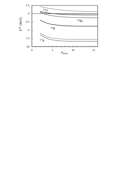
Figure 2: Ground-state energies (with respect to the core+n+n threshold) as a function of the maximum hypermomentum $K_{\rm max}$. The dotted lines are obtained by neglecting core excitations.

III.2 ¹⁴Be as a ¹²Be+n+n system

Before considering a full diagonalization of the basis, I first display the energy curves, where a single value of the generator coordinate $R$ is considered. The energy curves $E^{J\pi}_{i}(R)$ are therefore obtained from the eigenvalue problem

$$\sum_{K^{\prime}\gamma^{\prime}}\bigl{[}H^{J\pi}_{\gamma K,\gamma^{\prime}K^{\prime}}(R,R)-E^{J\pi}_{i}(R)N^{J\pi}_{\gamma K,\gamma^{\prime}K^{\prime}}(R,R)\bigr{]}$$

$$\hskip 28.45274pt\times f^{J\pi}_{\gamma^{\prime}K^{\prime}}=0,$$ (20)

where $N^{J\pi}_{\gamma K,\gamma^{\prime}K^{\prime}}(R,R^{\prime})$ is the overlap kernel. They provide a useful overview of the system. From the attractive or repulsive character, one can predict the existence of bound states (or of narrow resonances). In all cases, the three-body threshold is subtracted.

The ¹²Be+n+n energy curves are displayed in Fig. 3. In positive parity, there is a minimum for $J=0^{+}$ and $J=2^{+}$, which correspond to the ¹⁴Be ground state and to the $2^{+}$ resonance, respectively. In negative parity, the $0^{-}$ and $2^{-}$ curves are repulsive. There is a shallow minimum for $J=1^{-}$ which might be associated with a broad resonance. A deeper analysis of such resonances, however, would require a specific formalism for continuum states Damman and Descouvemont (2009), and is beyond the scope of the present work.

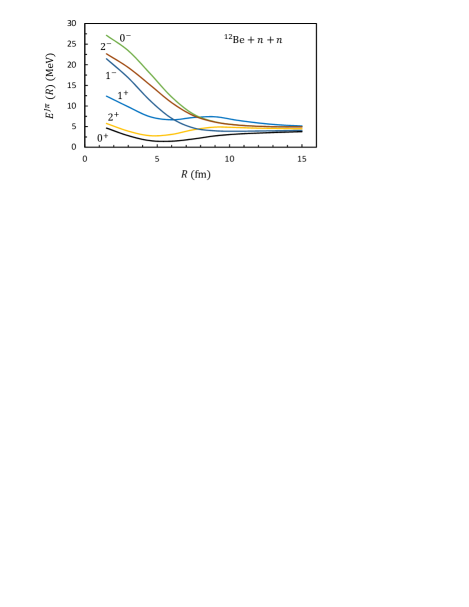
Figure 3: ¹²Be+n+n energy curves (20) for different $J\pi$-values.

An interesting characteristic of the system is provided by the energy convergence as a function of the maximum $R$ value, which I denote as $R_{\rm max}$. In Fig. 4, I show ¹⁴Be energies obtained by increasing the $N$ value in Eq. (16) or, in other words, by increasing $R_{\rm max}$. Two different behaviours can be clearly observed. The $0^{+}$ and $2^{+}$ energies are almost stable above $\mbox{$R_{\rm max}$}\approx 10$ fm, and present a plateau. The $2^{+}$ energy is 0.25 MeV, in nice agreement with experiment ($0.28\pm 0.01$ MeV Sugimoto et al. (2007)). This result emphasizes the importance of a microscopic theory; a non-microscopic three-body model, based on ¹²Be+n and on $n+n$ phenomenological interactions, does not reproduce the $0^{+}$ and $2^{+}$ energies simultaneously Descouvemont et al. (2006). The ¹²Be(g.s.)+n+n component is 87% in the ground state, and 67% in the $2^{+}$ resonance. This means that core excitations play a role, and may explain why non-microscopic models, which ignore core excitations, cannot predict the $2^{+}$ energy accurately. The other curves in Fig. 4 do not present a plateau, which means that no further narrow resonance can be expected. In particular, the $1^{-}$ curve is typical of a continuum state where, according to the variational principle, the minimum energy is zero.

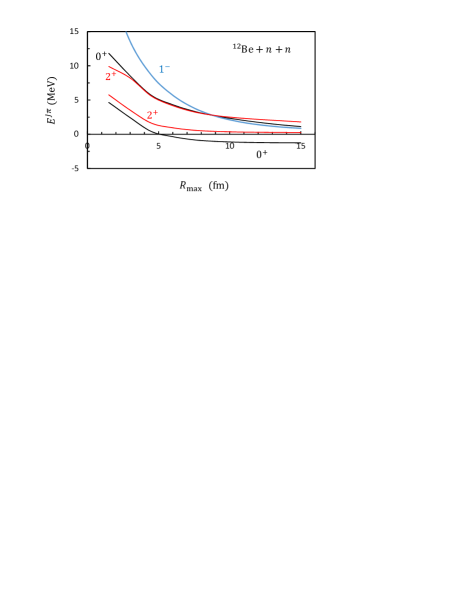
Figure 4: Convergence of ¹⁴Be energies with respect to the maximum generator coordinate $R_{\rm max}$.

Another useful method to distinguish between narrow and broad resonances is to analyze the convergence of the r.m.s. radius $\langle r^{2}\rangle$ as a function of $R_{\rm max}$. This is displayed in Fig. 5. The $0^{+}$ and $2^{+}$ low-lying states reach convergence near $\mbox{$R_{\rm max}$}\approx 12$ fm. In contrast, the second eigenvalues present a diverging behaviour at large $R_{\rm max}$. This is expected since, strictly speaking, matrix elements involving continuum states diverge. Although I cannot specifically address continuum states, this technique allows a clear distinction between narrow and broad resonances. It is consistent with the energy convergence shown in Fig. 4, and confirms that r.m.s. radii in the continuum should be considered very carefully.

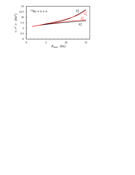
Figure 5: Convergence of the ¹⁴Be squared radius as a function of the maximum generator coordinate $R_{\rm max}$. The two first $0^{+}$ and $2^{+}$ eigenvalues are shown.

The ground-state radii are presented in Table 1, and compared with experiment. The neutron radius is in nice agreement with experiment. The experimental proton radius, however, is significantly larger than the predicted value. This is difficult to understand from a ¹²Be+n+n model, where the ¹⁴Be proton radius should be close to the core proton radius. Experimental values are partly model dependent, and a reanalysis of the ¹⁴Be charge radius would be welcome.

Table 1: Proton, neutron and matter radii (in fm).

	$\sqrt{<r^{2}>_{p}}$		$\sqrt{<r^{2}>_{n}}$		$\sqrt{<r^{2}>_{m}}$
	Th.	Exp.	Th.	Exp.	Th.	Exp.
14Be	2.10	$3.00(36)$	3.24	$3.22(39)$	2.96	$3.16(38)$
15B	2.23	$2.56(8)$	2.82		2.64	$2.75(6)$
17N	2.32		2.61		2.49	$2.48(5)$
17Ne	2.69	$3.04(2)$	2.32		2.54	$2.75(7)$
11Li	1.97	$2.467(37)$	3.12	$3.36(24)$	2.85	$3.27(24)$

Notice that the radii are slightly sensitive to the oscillator parameter $b$. From the total matter radius $\sqrt{<r^{2}>_{m}}$, one can define the expectation value of the hyperradius $<R^{2}>$ from

$$A<r^{2}_{m}>=A_{1}<r_{1}^{2}>+<R^{2}>,$$ (21)

where $\sqrt{<r_{1}^{2}>}$ is the core radius. In the shell model, this quantity is proportional to $b$ and takes the values $<r_{1}^{2}>=49b^{2}/24$ for ¹²Be, $<r_{1}^{2}>=27b^{2}/13$ for ¹³B, $<r_{1}^{2}>=32b^{2}/15$ for ¹⁵N and ¹⁵O, and $<r_{1}^{2}>=17b^{2}/9$ for ⁹Li. In contrast $<R^{2}>$, which is associated with the external neutrons, weakly depends on the oscillator parameter. For compact states, $<R^{2}>$ is small and the matter radius approximately varies linearly with $b$. For halo states, however, $<R^{2}>$ is the dominant term, and the matter radius is almost insensitive to the oscillator parameter.

III.3 ¹⁵B as a ¹³B+n+n system

The ¹⁵B ground state is known to be bound by 3.77 MeV. Although the spin assignment is no definite, there are strong indications for a spin $J=3/2^{-}$. Two excited states at $E_{x}=1.336$ MeV and $E_{x}=2.743$ MeV have been reported in Ref. Kanungo et al. (2005). On the theoretical side, shell-model Warburton and Brown (1992) and Antisymmetrized Molecular Dynamics (AMD, see Ref. Kanada-En’yo and Horiuchi (1995)) calculations have been performed. Non-microscopic calculations are unavailable until now, essentially due to the lack of reliable ¹³B+n potentials.

In Fig. 6, I present the energy curves of ¹⁵B. As expected, the lowest energy is obtained for $J=3/2^{-}$. I may also expect other bound states, corresponding to minima in the energy curves. The GCM spectrum, including all generator coordinates, is presented in Fig. 7. The theoretical spectrum shown inf Fig. 7 is remarkably supported by experiment Kanungo et al. (2005), although there is no spin assignment. The amount of ¹³B(g.s.)+n+n component is shown for the GCM calculation. As suggested by Fig. 6, the role of core excitation is small in ¹⁵B. As for ¹⁴Be, the positive-parity energy curves are not completely repulsive, but do not support narrow resonances. A more reliable study of positive-parity states in ¹⁵B would require introducing $sd$-shell components in the ¹³B wave functions. This would considerably increase the computer times, and is not feasible at the moment.

The proton and matter radii, given in Table 1 are in reasonable agreement with experiment. The theoretical radius of the ¹³B core is 2.31 fm, which means an increase of 0.33 fm for ¹⁵B.

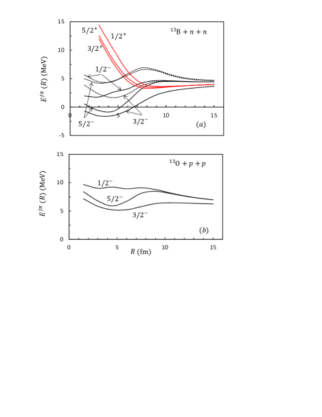
Figure 6: (a) ¹³B+n+n energy curves (20) for different $J\pi$-values. For negative parity, two eigenvalues are displayed. (b) ¹³O+p+p energy curves.

Let me briefly discuss the ¹⁵Ne mirror nucleus, which has been addressed experimentally in Ref. Wamers et al. (2014) and theoretically in Ref. Golubkova et al. (2016). The ground state and first excited state have been observed in two-neutron knockout reactions from a ¹⁷Ne beam at 2.5 and 4.4 MeV above the ¹³O+p+p threshold. Both states are expected to be broad.

In the present model, the ¹⁵B and ¹⁵Ne mirror nuclei are studied in the same conditions. The energy curves are shown in Fig. 6(b). The $3/2^{-}$ and $5/2^{-}$ curves present minima which are associated with the ground and first excited states. These minima are close to the Coulomb barrier, and clearly suggest continuum states. According to the higher centrifugal barrier, however, the $5/2^{-}$ excited state could be narrower than the $3/2^{-}$ ground state. The ¹⁵Ne spectrum is shown in Fig. 7. Although the GCM energies are obtained in the bound-state approximation, the results are close to the energies observed experimentally Wamers et al. (2014).

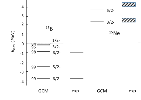
Figure 7: ¹⁵B and ¹⁵Ne energy spectra, compared with experiment Kanungo et al. (2005); Wamers et al. (2014). Numbers at the left of the GCM states correspond to the amount of ¹³B(g.s.)+n+n configuration (in %). For ¹⁵Ne, the hatched areas indicate broad resonances.

III.4 ¹⁷N as ¹⁵N+n+n and ¹⁷Ne as ¹⁵O+p+p systems

Microscopic calculations involving a ¹⁵N or a ¹⁵O core are relatively simple since only the ground state $1/2^{-}$ and the first excited state $3/2^{-}$ are present in the $0\hbar\omega$ shell model. A previous three-cluster microscopic calculation was performed in Ref. Timofeyuk et al. (1996), where the main goal was to address the possible existence of a proton halo in ¹⁷Ne. Figure 8 shows the energy curves, which present a minimum near $R=0$ for negative parity. This suggests a compact structure for negative-parity states, in contrast with the other systems considered here.

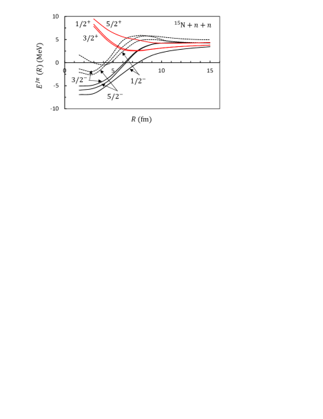
Figure 8: ¹⁵N+n+n energy curves (20) for different $J\pi$-values.

The ¹⁷N spectrum is displayed in Fig. 9. The general agreement with experiment is reasonable but, as in Ref. Timofeyuk et al. (1996) the ordering of the two first excited states is incorrect. For all states the ¹⁵N(g.s.)+n+n component is dominant. No positive parity state is found, as suggested by the repulsive energy curves of Fig. 8.

The ¹⁷Ne spectrum is studied with the same nucleon-nucleon interaction; the Majorana parameter is the same as in ¹⁷N. The GCM reproduces the binding energy very well ($-1.05$ MeV in the model, to be compared to the experimental value $-0.93$ MeV), which shows that the Coulomb shift is accurately described.

Electromagnetic transitions have been suggested to be a valuable tool to investigate the structure of ¹⁷Ne Grigorenko et al. (2005); Fortune (2018). The E2 transition probabilities have been studied by relativistic Coulomb excitation with a ¹⁷Ne radioactive beam Chromik et al. (1997, 2002); Marganiec et al. (2016). The $B(E2)$ values, computed without any effective charge, are presented in Table 2. The $B(E2,1/2^{-}\rightarrow 5/2^{-})$ GCM value is in excellent agreement with the latest data of Marganiec et al. Marganiec et al. (2016). The experimental value of Chromik et al. Chromik et al. (2002) is larger, but is probably influenced by nuclear effects which have been dismissed in the analysis Marganiec et al. (2016). The transition to the $3/2^{-}$ state is also well reproduced, which shows that the GCM wave functions are reliable.

Table 2: E2 electromagnetic transition probabilities (in $e^{2}$.fm⁴) in ¹⁷Ne. No effective charge is used.

	GCM	Exp.
$1/2^{-}\rightarrow 5/2^{-}$	92.9	$90\pm 18$ Marganiec et al. (2016), $124\pm 18$ Chromik et al. (2002)
$1/2^{-}\rightarrow 3/2^{-}$	68.0	$68^{+19}_{-25}$ Chromik et al. (1997)
$5/2^{-}\rightarrow 3/2^{-}$	7.1

The matter radius of the ¹⁷N ground state, given in Table 1, is an excellent agreement with experiment Ozawa et al. (1994). For ¹⁷Ne, however, even if the binding energy is lower, the GCM does not support the large difference with ¹⁷N. I rather confirm the conclusion of Ref. Timofeyuk et al. (1996), that there is no evidence for a proton halo in ¹⁷Ne.

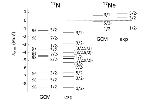
Figure 9: ¹⁷N and ¹⁷Ne energy spectra, compared with experiment Tilley et al. (1993). Only negative-parity states are shown. Numbers at the left of GCM states correspond to the amount of ¹⁵N(g.s.)+n+n configuration (in %).

III.5 ¹¹Li as a ⁹Li+n+n system

The ¹¹Li nucleus has been studied in many experimental and theoretical works. The very low binding energy ($S_{2n}=0.367$ MeV Audi et al. (2017)) is responsible for a remarkable halo structure, as suggested by the large r.m.s. radius. The present calculation is made difficult because of the large number of Slater determinants (90) involved in the ⁹Li core. A previous microscopic three-cluster study was performed in Ref. Descouvemont (1997), but with a frozen triangular geometry. In Ref. Varga et al. (2002), the authors describe the core in an $\alpha+t+n+n$ multicluster configuration.

The ⁹Li+n+n energy curves are displayed in Fig. 10. A minimum is obtained for $J=3/2^{-}$ and, to a lesser extend, for $J=1/2^{-}$. The $3/2^{-}$ minimum corresponds to the ¹¹Li ground state. The role of core excitations is illustrated in Fig. 2. When core excitations are neglected, the state is unbound. The importance of core excitations was already pointed out in Ref. Varga et al. (2002). In contrast with the previous examples, where the neutron number of the core $N=8$ corresponds to a closed shell, the various ⁹Li+n+n configurations are not orthogonal to each other. Consequently, a ground-state component in ¹¹Li cannot be estimated.

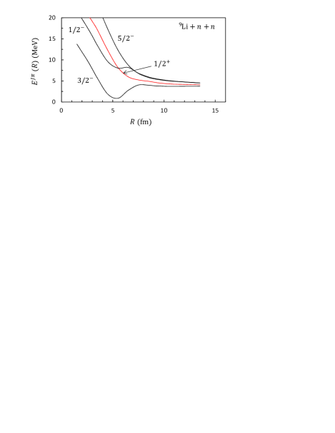
Figure 10: ⁹Li+n+n energy curves (20) for different $J\pi$-values.

The proton, neutron and matter radii are presented in Table 1. The calculation confirms the large enhancement of the matter radius, compared to the ⁹Li core (the shell-model value is $\sqrt{<r^{2}>_{m}}(^{9}{\rm Li})=b\sqrt{17/9}=2.20$ fm). The GCM value is, however, slightly smaller than experiment. For the proton radius, the experimental ¹¹Li value (2.467 fm) is significantly larger than the ⁹Li value (2.217 fm), which suggests that the neutron halo of ¹¹Li affects the core Sánchez et al. (2006); Puchalski et al. (2006). In the present model, the ⁹Li proton radius is $\sqrt{<r^{2}>_{p}}(^{9}{\rm Li})=b\sqrt{4/3}=1.84$ fm. The difference between ¹¹Li and ⁹Li is therefore 0.13 fm, which is smaller than experiment (0.25 fm) (see a detailed discussion in Refs. Sánchez et al. (2006); Puchalski et al. (2006)).

IV Conclusion

The main goal of the present work is to extend the hyperspherical formalism to microscopic three-cluster models. The hyperradial functions are expanded over a Gaussian basis using the Generator Coordinate method. Then the wave functions are expressed in terms of projected Slater determinants. This approach is well adapted to multicluster systems. With a single generator coordinate, it provides an accurate description of the wave functions, even at long distances. The calculations of the matrix elements, however, require very long computer times, owing to the seven-dimension integrals necessary for the angular momentum projection. The extension to $p$-shell cores raises additional difficulties due to $(i)$ the quadruple sums involved in the matrix elements of two-body interactions; $(ii)$ the presence of several Slater determinants; $(iii)$ the introduction of core excited states. The calculations are made possible thanks to an efficient parallelization of the computer code.

The model has been applied to some exotic light nuclei: ¹⁴Be, ¹⁵B, ¹⁷Ne and ¹¹Li. In all cases, the only parameter (the admixture parameter $M$ involved in the Volkov nucleon-nucleon interaction) is adjusted on the ground-state energy. For ¹⁴Be, the $2^{+}$ excitation energy is well reproduced, in contrast with non-microscopic models. The GCM spectrum of ¹⁵B is in nice agreement with the experimental energies. An exploratory study of the ¹⁵Ne mirror system, which is unbound, is consistent with the experimental energies, and suggests that the first excited state is narrower than the ground state. The ¹⁷N spectrum presents many states which, in general, are fairly well reproduced by the GCM. The ground state is confirmed to be $1/2^{-}$, but the order of the first two excited states in incorrect, as in Ref. Timofeyuk et al. (1996). In the ¹⁷Ne mirror nucleus, the ground-state energy, as well as E2 transition probabilities are in good agreement with experiment. For ¹¹Li, calculations are extremely long, owing to the 90 Slater determinants involved in the core. The neutron and matter radii are explained fairly well, but the proton radius is smaller than the experimental value.

The present model could be extended to deal with three-body continuum states Damman and Descouvemont (2009). On the other hand, the wave functions could be used as an input to determine scattering cross sections, as it was done for ⁶He for example Descouvemont (2016).

Appendix A Core wave functions

In this Appendix I give some detail about the core wave functions (5). The quantum numbers ($I,L,S,T$) are given in Table 3. First, the list of functions $\bar{\Phi}_{i}$ is determined, and is then used to diagonalize the operators $\boldsymbol{I}^{2},\boldsymbol{L}^{2},\boldsymbol{S}^{2}$ and $\boldsymbol{T}^{2}$. The diagonalization provides eigenvalues and coefficients $d^{I\nu LST}_{i}$, which do not depend on the Hamiltonian.

Table 3: Quantum numbers ($I,L,S,T$) of the core wave functions. $n$ is the degeneracy.

	$I$	$T$	$S$	$L$	$n$
9Li	1/2	3/2	1/2	0	1
				1	2
			3/2	1	1
				2	2
		5/2	1/2	1	1
	3/2	3/2	1/2	1	2
				2	2
			3/2	0	1
				1	1
				2	1
		5/2	1/2	1	1
	5/2	3/2	1/2	2	2
				3	1
			3/2	1	1
				2	1
	7/2	3/2	1/2	3	1
			3/2	2	1
12Be	0	2	0	0	1
			1	1	1
	1	2	1	1	1
	2	2	0	2	1
			1	2	1
13B	1/2	3/2	1/2	1	1
	3/2	3/2	1/2	1	1
			1/2	2	1
			3/2	0	1
	5/2	3/2	1/2	2	1
15N	1/2	1/2	1/2	1	1
	3/2	1/2	1/2	1	1

References

- Tanihata et al. (2013) I. Tanihata, H. Savajols, and R. Kanungo, Prog. Part. Nucl. Phys. 68, 215 (2013).
- Lin (1995) C. D. Lin, Phys. Rep. 257, 1 (1995).
- Gattobigio et al. (2011) M. Gattobigio, A. Kievsky, and M. Viviani, Phys. Rev. C 83, 024001 (2011).
- Descouvemont and Dufour (2012) P. Descouvemont and M. Dufour, Clusters in Nuclei, edited by C. Beck, Vol. 2 (Springer, 2012).
- Horiuchi et al. (2012) H. Horiuchi, K. Ikeda, and K. Katō, Progress of Theoretical Physics Supplement 192, 1 (2012).
- Filippov et al. (1996) G. F. Filippov, K. Katō, and S. V. Korennov, Prog. Theor. Phys. 96, 575 (1996).
- Korennov and Descouvemont (2004) S. Korennov and P. Descouvemont, Nucl. Phys. A 740, 249 (2004).
- Damman and Descouvemont (2009) A. Damman and P. Descouvemont, Phys. Rev. C 80, 044310 (2009).
- Descouvemont (2016) P. Descouvemont, Phys. Rev. C 93, 034616 (2016).
- Descouvemont and Pinilla (2019) P. Descouvemont and E. C. Pinilla, Few-Body Systems 60, 11 (2019).
- Blumenfeld et al. (2013) Y. Blumenfeld, T. Nilsson, and P. Van Duppen, Physica Scripta 2013, 014023 (2013).
- Wildermuth and Tang (1977) K. Wildermuth and Y. C. Tang, A Unified Theory of the Nucleus, edited by K. Wildermuth and P. Kramer (Vieweg, Braunschweig, 1977).
- Volkov (1965) A. B. Volkov, Nucl. Phys. 74, 33 (1965).
- Thompson et al. (1977) D. R. Thompson, M. LeMere, and Y. C. Tang, Nucl. Phys. A 286, 53 (1977).
- Machleidt et al. (2013) R. Machleidt, Q. MacPherson, E. Marji, R. Winzer, C. Zeoli, and D. R. Entem, Few-Body Systems 54, 821 (2013).
- Kanada-En’yo and Akaishi (2004) Y. Kanada-En’yo and Y. Akaishi, Phys. Rev. C 69, 034306 (2004).
- Itagaki (2016) N. Itagaki, Phys. Rev. C 94, 064324 (2016).
- Horiuchi (1977) H. Horiuchi, Prog. Theor. Phys. Suppl. 62, 90 (1977).
- Descouvemont (1995) P. Descouvemont, Nucl. Phys. A 584, 532 (1995).
- Descouvemont (2004) P. Descouvemont, Phys. Rev. C 70, 065802 (2004).
- Zhukov et al. (1993) M. V. Zhukov, B. V. Danilin, D. V. Fedorov, J. M. Bang, I. J. Thompson, and J. S. Vaagen, Phys. Rep. 231, 151 (1993).
- Kievsky et al. (2008) A. Kievsky, S. Rosati, M. Viviani, L. E. Marcucci, and L. Girlanda, J. Phys. G 35, 063101 (2008).
- Descouvemont and Baye (1994) P. Descouvemont and D. Baye, Nucl. Phys. A 573, 28 (1994).
- Audi et al. (2017) G. Audi, F. G. Kondev, M. Wang, W. Huang, and S. Naimi, Chin. Phys. C 41, 030001 (2017).
- Sugimoto et al. (2007) T. Sugimoto, T. Nakamura, Y. Kondo, N. Aoi, H. Baba, D. Bazin, N. Fukuda, T. Gomi, H. Hasegawa, N. Imai, M. Ishihara, T. Kobayashi, T. Kubo, M. Miura, T. Motobayashi, H. Otsu, A. Saito, H. Sakurai, S. Shimoura, A. Vinodkumar, K. Watanabe, Y. Watanabe, T. Yakushiji, Y. Yanagisawa, and K. Yoneda, Phys. Lett. B 654, 160 (2007).
- Descouvemont et al. (2006) P. Descouvemont, E. M. Tursunov, and D. Baye, Nucl. Phys. A 765, 370 (2006).
- Tanihata et al. (1988) I. Tanihata, T. Kobayashi, O. Yamakawa, S. Shimoura, K. Ekuni, K. Sugimoto, N. Takahashi, T. Shimoda, and H. Sato, Phys. Lett. B 206, 592 (1988).
- Estradé et al. (2014) A. Estradé, R. Kanungo, W. Horiuchi, F. Ameil, J. Atkinson, Y. Ayyad, D. Cortina-Gil, I. Dillmann, A. Evdokimov, F. Farinon, H. Geissel, G. Guastalla, R. Janik, M. Kimura, R. Knöbel, J. Kurcewicz, Y. A. Litvinov, M. Marta, M. Mostazo, I. Mukha, C. Nociforo, H. J. Ong, S. Pietri, A. Prochazka, C. Scheidenberger, B. Sitar, P. Strmen, Y. Suzuki, M. Takechi, J. Tanaka, I. Tanihata, S. Terashima, J. Vargas, H. Weick, and J. S. Winfield, Phys. Rev. Lett. 113, 132501 (2014).
- Ozawa et al. (1994) A. Ozawa, T. Kobayashi, H. Sato, D. Hirata, I. Tanihata, O. Yamakawa, K. Omata, K. Sugimoto, D. Olson, W. Christie, and H. Wieman, Phys. Lett. B 334, 18 (1994).
- Geithner et al. (2008) W. Geithner, T. Neff, G. Audi, K. Blaum, P. Delahaye, H. Feldmeier, S. George, C. Guénaut, F. Herfurth, A. Herlert, S. Kappertz, M. Keim, A. Kellerbauer, H.-J. Kluge, M. Kowalska, P. Lievens, D. Lunney, K. Marinova, R. Neugart, L. Schweikhard, S. Wilbert, and C. Yazidjian, Phys. Rev. Lett. 101, 252502 (2008).
- Sánchez et al. (2006) R. Sánchez, W. Nörtershäuser, G. Ewald, D. Albers, J. Behr, P. Bricault, B. A. Bushaw, A. Dax, J. Dilling, M. Dombsky, G. W. F. Drake, S. Götte, R. Kirchner, H.-J. Kluge, T. Kühl, J. Lassen, C. D. P. Levy, M. R. Pearson, E. J. Prime, V. Ryjkov, A. Wojtaszek, Z.-C. Yan, and C. Zimmermann, Phys. Rev. Lett. 96, 033002 (2006).
- Tanihata et al. (1985) I. Tanihata, H. Hamagaki, O. Hashimoto, Y. Shida, N. Yoshikawa, K. Sugimoto, O. Yamakawa, T. Kobayashi, and N. Takahashi, Phys. Rev. Lett. 55, 2676 (1985).
- Kanungo et al. (2005) R. Kanungo, Z. Elekes, H. Baba, Z. Dombrádi, Z. Fūlōp, J. Gibelin, . Horváth, Y. Ichikawa, E. Ideguchi, N. Iwasa, H. Iwasaki, S. Kawai, Y. Kondo, T. Motobayashi, M. Notani, T. Ohnishi, A. Ozawa, H. Sakurai, S. Shimoura, E. Takeshita, S. Takeuchi, I. Tanihata, Y. Togano, C. Wu, Y. Yamaguchi, Y. Yanagisawa, A. Yoshida, and K. Yoshida, Phys. Lett. B 608, 206 (2005).
- Warburton and Brown (1992) E. K. Warburton and B. A. Brown, Phys. Rev. C 46, 923 (1992).
- Kanada-En’yo and Horiuchi (1995) Y. Kanada-En’yo and H. Horiuchi, Phys. Rev. C 52, 647 (1995).
- Wamers et al. (2014) F. Wamers, J. Marganiec, F. Aksouh, Y. Aksyutina, H. Álvarez-Pol, T. Aumann, S. Beceiro-Novo, K. Boretzky, M. J. G. Borge, M. Chartier, A. Chatillon, L. V. Chulkov, D. Cortina-Gil, H. Emling, O. Ershova, L. M. Fraile, H. O. U. Fynbo, D. Galaviz, H. Geissel, M. Heil, D. H. H. Hoffmann, H. T. Johansson, B. Jonson, C. Karagiannis, O. A. Kiselev, J. V. Kratz, R. Kulessa, N. Kurz, C. Langer, M. Lantz, T. Le Bleis, R. Lemmon, Y. A. Litvinov, K. Mahata, C. Müntz, T. Nilsson, C. Nociforo, G. Nyman, W. Ott, V. Panin, S. Paschalis, A. Perea, R. Plag, R. Reifarth, A. Richter, C. Rodriguez-Tajes, D. Rossi, K. Riisager, D. Savran, G. Schrieder, H. Simon, J. Stroth, K. Sümmerer, O. Tengblad, H. Weick, C. Wimmer, and M. V. Zhukov, Phys. Rev. Lett. 112, 132502 (2014).
- Golubkova et al. (2016) T. Golubkova, X.-D. Xu, L. Grigorenko, I. Mukha, C. Scheidenberger, and M. Zhukov, Phys. Lett. B 762, 263 (2016).
- Timofeyuk et al. (1996) N. Timofeyuk, P. Descouvemont, and D. Baye, Nucl. Phys. A 600, 1 (1996).
- Grigorenko et al. (2005) L. V. Grigorenko, Y. L. Parfenova, and M. V. Zhukov, Phys. Rev. C 71, 051604 (2005).
- Fortune (2018) H. T. Fortune, Phys. Rev. C 97, 014308 (2018).
- Chromik et al. (1997) M. J. Chromik, B. A. Brown, M. Fauerbach, T. Glasmacher, R. Ibbotson, H. Scheit, M. Thoennessen, and P. G. Thirolf, Phys. Rev. C 55, 1676 (1997).
- Chromik et al. (2002) M. J. Chromik, P. G. Thirolf, M. Thoennessen, B. A. Brown, T. Davinson, D. Gassmann, P. Heckman, J. Prisciandaro, P. Reiter, E. Tryggestad, and P. J. Woods, Phys. Rev. C 66, 024313 (2002).
- Marganiec et al. (2016) J. Marganiec, F. Wamers, F. Aksouh, Y. Aksyutina, H. Álvarez-Pol, T. Aumann, S. Beceiro-Novo, C. Bertulani, K. Boretzky, M. Borge, M. Chartier, A. Chatillon, L. Chulkov, D. Cortina-Gil, H. Emling, O. Ershova, L. Fraile, H. Fynbo, D. Galaviz, H. Geissel, M. Heil, D. Hoffmann, J. Hoffmann, H. Johansson, B. Jonson, C. Karagiannis, O. Kiselev, J. Kratz, R. Kulessa, N. Kurz, C. Langer, M. Lantz, T. L. Bleis, R. Lemmon, Y. Litvinov, K. Mahata, C. Müntz, T. Nilsson, C. Nociforo, G. Nyman, W. Ott, V. Panin, S. Paschalis, A. Perea, R. Plag, R. Reifarth, A. Richter, C. Rodriguez-Tajes, D. Rossi, K. Riisager, D. Savran, G. Schrieder, H. Simon, J. Stroth, K. Sümmerer, O. Tengblad, S. Typel, H. Weick, M. Wiescher, and C. Wimmer, Phys. Lett. B 759, 200 (2016).
- Tilley et al. (1993) D. R. Tilley, H. R. Weller, and C. M. Cheves, Nucl. Phys. A 564, 1 (1993).
- Descouvemont (1997) P. Descouvemont, Nucl. Phys. A 626, 647 (1997).
- Varga et al. (2002) K. Varga, Y. Suzuki, and R. G. Lovas, Phys. Rev. C 66, 041302 (2002).
- Puchalski et al. (2006) M. Puchalski, A. M. Moro, and K. Pachucki, Phys. Rev. Lett. 97, 133001 (2006).