A novel Algorithm for Optimal Placement of Multiple Inertial Sensors to Improve the Sensing Accuracy

Abstract

This paper proposes a novel algorithm to determine the optimal placement of redundant inertial sensors such as accelerometers and gyroscopes (gyros) for increasing the sensing accuracy. In this paper, we have proposed a novel iterative algorithm to find the optimal sensor configuration. The proposed algorithm utilizes the majorization-minimization (MM) algorithm and the duality principle to find the optimal configuration. Unlike the state-of-the-art which are mainly geometrical in nature and restricted to certain noise statistics, the proposed algorithm gives the exact positions of the sensors, and moreover, the proposed algorithm is independent of the nature of the noise at different sensors. The proposed alogrithm has been implemented and tested via numerical simulation in the MATLAB. The simulation results show that the algorithm converges to the optimal configurations and show the effectiveness of the proposed algorithm.

I Introduction and Literature

An inertial navigation system (INS) calculates the navigation solution such as position, velocity, and attitude (PVA) of a navigating platform based on the initial PVA and by processing the measurements from inertial measurement unit (IMU) using navigation equations. An IMU is made of three mutually orthogonal accelerometers and three gyroscopes (gyros) aligned with the accelerometers. An accelerometer measures the specific force and gyro measures the angular velocity. The specific force accounts the acceleration due to all forces except for the gravity [1]. An INS requires at least three accelerometers and three gyros for computing the navigation solutions; however, using redundant sensors ensure the reliability and enhance the navigation accuracy. In a redundant inertial measurement unit (RIMU), more than three gyroscopes or accelerometers are used to handle the sensor failure or malfunction. When some sensors malfunction, the faulty sensors should be identified and removed so that the navigation system with the RIMU continues to operate normally. Using redundant sensors also enhance the performance of an IMU because the additional information from the redundant sensors would increase the sensing accuracy of the IMU [2]. However, using redundant inertial sensors creates the problem of placement of sensors and orientation of the sensing axis. Here, in this paper we will investigate the problem of optimal configuration of redundant sensors to improve the sensing accuracy.

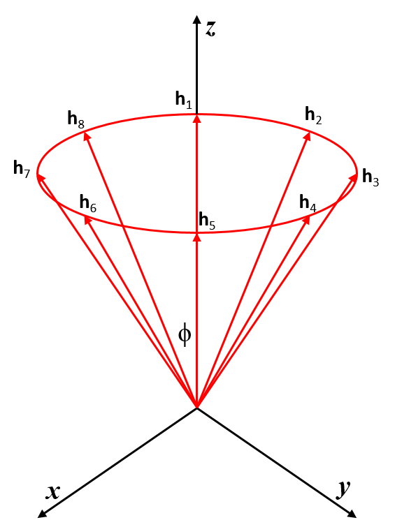
(a) Class-I configuration for eight sensors.

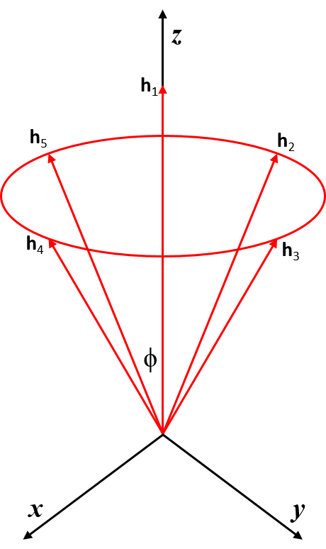
(b) Class-II configuration for five sensors.

Figure 1: Class-I and class-II optimal configurations.

The accuracy analysis of the configuration of sensors having noise with mean zero and equal variances is described in [3]. In [3], the author has proposed two geometries for redundant sensor configuration as shown in figure 1. In the class-I optimal configuration, the sensors’ sensing axis are equally spaced on a cone with half-angle $\phi=\arccos\left(\nicefrac{{1}}{{\sqrt{3}}}\right)$. Figure 1a depicts the class-I configuration for eight sensors. In the class-II optimal configuration, the sensing axis of one of the $m$ sensors is placed along cone axis and the remaining $m-1$ sensors’ sensing axis are equally spread on a cone having half angle $\phi$ satisfying $\cos^{2}\left(\phi\right)=\nicefrac{{\left(m-1\right)}}{{\left(3m-3\right)}}$, where $m$ being the total number of sensors. Figure 1b depicts the class-II configuration for five sensors in which the sensing axis $\mathbf{h}_{1}$ is placed along the cone axis and the remaining four sensing axis, $\mathbf{h}_{2}$ to $\mathbf{h}_{5}$, are equally spread on the cone. In [4], the authors have presented the configurations of redundant inertial sensors for improving the navigation performance and for the fault detection and isolation (FDI) capability; to rank the redundant sensor configuration for navigation performance, the volume of the ellipsoid associated with the estimation error covariance matrix, that is, the determinant of the error covariance matrix has been taken as figure of merit (FOM). The determinant of the error covariance matrix has also been used as a FOM in [5], the configuration of sensors has been proposed considering reliability, navigation accuracy, size and cost of the system. In [6], the configuration of redundant sensors has been studied for improving sensing accuracy and detecting faulty sensors. The author in [6] has defined the regular polyhedra (platonic solids) and described the existence of only five regular polyhedra. The platonic solids have congruent regular polygonal faces and same number of faces meet at each vertex. It has been suggested that if sensor axes are placed along the normals to the faces of regular ployhedra they form the optimal configuration for optimal sensing. In [6], geometric dilution of precision (GDOP) which is defined as the square root of the trace of the estimation error covariance matrix has been used as FOM to analyze the redundant sensor configurations. The criterion of minimum GDOP as FOM to analyze the cone configurations has also been used in [7], [8]. The idea of maximizing the determinant of the information matrix, which is the inverse of the estimation error covariance matrix, has been used in [9], [10] to determine the optimal configuration of any number of sensors. The author in [11] has proposed the partial redundancy method to determine the optimal configuration of multiple IMUs, which is based on the concept of reliability and is typically applied in the geodetic network. In [11], it has been shown that for IMU triads, their optimal configuration is independent of the geometry between them. The optimal sensor configuration which considers both the navigation and FDI performances has been discussed in [12]; a necessary and sufficient condition which a configuration must satisfy for optimal navigation performance has been given, and a FOM for sensor configuration which considers both the navigation and FDI performance has been suggested. The criterion is that among the optimal sensor configurations for navigation performance, the optimal configuration for FDI performance is the one which makes the angle between the nearest two sensors the largest. The authors in [2] have proposed a configuration in which the orientation of redundant sensors is such that it provides the best navigation performance and their location minimizes the lever arm effect. The lever arm effect is generated when the center of gravity of each sensor deviates from the origin of the case frame. In [2], the maximum eigenvalue of the estimation error covariance matrix has been taken as the FOM to determine the optimal sensor orientation for best navigation performance.

I-A Our Contribution

From the literature survey, it was observed that optimal orientations are discussed for sensors having uncorrelated and equal variances of random noise. The optimal configurations for such sensors are proposed to be the platonic solids and sensors placed on a cone (class-I and class-II configuration) etc. No methods/approaches are available to optimally place the sensing axis of sensors having correlated and/or different variances of noise. So one can think of that what would be the optimal configuration for sensors having different accuracies. Here, we have proposed a numerical algorithm to find the optimal configuration of sensors having correlated and different variances of noise. The proposed algorithm is based on the MM algorithm and the duality theory from optimization. The proposed algorithm can find the optimal configuration for any noise configuration. The convergence analysis, computational complexity and the numerical results of the proposed algorithm are also discussed.

I-B Assumptions and Notations

In this study, the lever arms are not considered that is their placement is not considered only orientation has been discussed. The only source of error in sensor measurement is random noise. The systematic errors are assumed to be calibrated. The variances of random noise in each sensor are not the same, and the noise at the sensors are assumed to be correlated.

Throughout this paper the italic small letters are used for scalars, boldface small letters for vectors and boldface capital letters for matrices. $\left(.\right)^{T}$, $\left(.\right)^{-1}$ and $\left\|.\right\|_{2}$ denote the transpose, inverse and Euclidean norm or $l_{2}-$norm, respectively. $\mathbb{E}\left(.\right)$, $\det\left(.\right)$, $\log\left(.\right)$ and $\mathrm{Tr}\left(.\right)$ represent the expectation, determinant, logarithm and trace operators, respectively. $\mathbb{R}^{n}$ and $\mathbb{S}_{+}^{n}$denote the $n-$dimensional Euclidean space and the set of $n\times n$ symmetric positive semidefinite matrices respectively. Notation $\mathbf{A}\succeq\mathbf{B}$ stands for matrix $\mathbf{A}-\mathbf{B}$ is positive semidefinite. $\mathbf{x}_{t}$ stands for the value of $\mathbf{x}$ at the $t-$th iteration and $x_{i}^{t}$ denotes the value of the $i^{th}$ element of $\mathbf{x}_{t}$.

In section II, we discuss the problem of placing the sensors in optimal configuration and form the optimization problems whose optimal solution gives the optimal configuration. In section III, we describe the MM algorithm, the proposed algorithm which solves the optimization problems formulated in section II, convergence analysis and computational complexity. Simulation results are reported in section IV. Finally the paper concludes in section V.

II Problem Formulation

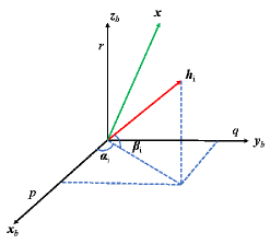
Figure 2: Orientation of the single axis inertial sensors

We have the inertial quantity $\mathbf{x}=\left(\begin{array}[]{ccc}p&q&r\end{array}\right)^{T}$ which is either acceleration or angular velocity to be measured. This inertial quantity is to be measured with $m\left(\geq 3\right)$ single axis inertial sensors. The gyro and accelerometer measurements are considered separately. For optimal sensing of the inertial quantity $\mathbf{x}$, we have to find the optimal configuration of these $m$ sensors with respect to some reference frame generally taken as the vehicle body frame ($b-$frame). In figure 2, $x_{b}$, $y_{b}$, and $z_{b}$ are the axes of the $b-$frame.

The unit vector along the sensitive axis of the $i^{th}$ inertial sensor can be represented in Cartesian coordinate as $\mathbf{h}_{i}\in\mathbb{R}^{n\times 1}$ with $n=3$ and $\mathbf{h}_{i}^{T}\mathbf{h}_{i}=1$.

Let $y_{i}$ denote the component of $\mathbf{x}$ along $\mathbf{h}_{i}$, the sensitive axis of the $i^{th}$sensor, then $y_{i}$ can be written as:

$$y_{i}=\mathbf{h}_{i}^{T}\mathbf{x}.$$ (1)

The actual measurement of $y_{i}$ by the $i^{th}$ sensor with error, denoted as $\widetilde{y}_{i}$, is given by:

$$\widetilde{y}_{i}=\mathbf{h}_{i}^{T}\mathbf{x}+\varepsilon_{i},$$ (2)

where $\varepsilon_{i}$ is the zero mean Gaussian random noise with variance $\sigma_{i}^{2}$, i.e. $\varepsilon_{i}\thicksim N\left(0,\sigma_{i}^{2}\right)$. The measurements from $m$ redundant inertial sensors can be written as:

$$\left(\begin{array}[]{c}\widetilde{y}_{1}\\ :\\ :\\ \widetilde{y}_{m}\end{array}\right)=\left(\begin{array}[]{c}\mathbf{h}_{1}^{T}\\ :\\ :\\ \mathbf{h}_{m}^{T}\end{array}\right)\mathbf{x}+\left(\begin{array}[]{c}\varepsilon_{1}\\ :\\ :\\ \varepsilon_{m}\end{array}\right).$$ (3)

In vector-matrix form, the above relation can be written as:

$$\widetilde{\mathbf{y}}=\mathbf{H}\mathbf{x}+\boldsymbol{\varepsilon}.$$ (4)

Here $\widetilde{\mathbf{y}}\in\mathbb{R}^{m\times 1}$ is the measurement vector, $\mathbf{H}\in\mathbb{R}^{m\times n}$ with $n=3$ is the measurement matrix with $\operatorname{rank}\left(\mathbf{H}\right)=3$, and $\boldsymbol{\varepsilon}$ is the measurement noise vector which is Gaussian with mean zero, that is, $\mathbb{E}\left(\boldsymbol{\varepsilon}\right)=0$ and covariance matrix $\mathbf{R}\in\mathbb{S}_{+}^{m}$, given by $\mathbf{R}=\mathbb{E}\left(\boldsymbol{\varepsilon}\boldsymbol{\varepsilon}^{T}\right)$.

The weighted least square estimate of $\mathbf{x}$, denoted as $\hat{\mathbf{x}}$, is given by:

$$\hat{\mathbf{x}}=\left(\mathbf{H}^{T}\mathbf{R}^{-1}\mathbf{H}\right)^{-1}\mathbf{H}^{T}\mathbf{R}^{-1}\mathbf{\widetilde{\mathbf{y}}}.$$ (5)

The estimation error, denoted as $\mathbf{e}$, is given by:

$$\mathbf{e}=\hat{\mathbf{x}}-\mathbf{x}=\left(\mathbf{H}^{T}\mathbf{R}^{-1}\mathbf{H}\right)^{-1}\mathbf{H}^{T}\mathbf{R}^{-1}\boldsymbol{\varepsilon}.$$ (6)

The estimation error covariance matrix would be:

$$\mathbf{C}_{e}=\mathbb{E}\left(\left(\boldsymbol{\hat{\mathbf{x}}-\mathbf{x}}\right)\left(\boldsymbol{\hat{\mathbf{x}}-\mathbf{x}}\right)^{T}\right)=\left(\mathbf{H}^{T}\mathbf{R}^{-1}\mathbf{H}\right)^{-1}.$$ (7)

Since $\boldsymbol{\varepsilon}$ is Gaussian distributed with zero mean and any linear transformation does not change the Gaussian property, therefore, the estimation error $\mathbf{e}$, in (6) is also zero mean Gaussian distributed, hence, $\mathbf{e}\sim N\left(0,\mathbf{C}_{e}\right)$. The error covariance matrix characterizes the confidence of the estimation. The accuracy of the navigation solution of the INS depends on the error covariance matrix. From (7), we observe that the estimation error covariance matrix $\mathbf{C}_{e}$ depends on sensor configuration matrix $\mathbf{H}$ and the covariance matrix $\mathbf{R}$ of the measurement noise. Since $\mathbf{R}$ is fixed, we can choose the $\mathbf{H}$ in such a way that the error covariance matrix is small in some sense. There are various scalar metrics available which characterizes the size of the covariance matrix such as determinant, trace etc. The probability density function for the estimation error, $\mathbf{e}$, in (6) can be written as:

$$f_{\mathbf{e}}\left(\mathbf{e}\right)=\left(2\pi\right)^{-n/2}det\left(\mathbf{C}_{e}\right)^{-1/2}\exp\left(-\frac{1}{2}\mathbf{e}^{T}\mathbf{C}_{e}^{-1}\mathbf{e}\right).$$ (8)

The equidensity contours of any multivariate Gaussian distribution form ellipsoid. The locus of points $\mathbf{e}$ defined by $\mathbf{e}^{T}\mathbf{C}_{e}^{-1}\mathbf{e}=k$ forms an ellipsoid, on which the probability density is constant. For a given $k$ the volume of this ellipsoid is given by [4]:

$$V=\frac{4}{3}k^{3/2}\pi\sqrt{\det\left(\mathbf{C}_{e}\right)}.$$ (9)

From (9) we see that the volume of the error ellipsoid is proportional to the $\det\left(\mathbf{C}_{e}\right)$. Smaller the volume of the error ellipsoid, smaller is the estimation error and better is the estimate obtained using the sensor configuration. So minimizing the determinant of the error covariance matrix can be taken as a criterion to find the optimal configuration.

So, to find the optimal configuration of the inertial sensors, we can minimize the determinant of the error covariance matrix. This is called the $D-$optimal design [13]. This is equivalent to minimizing the volume of the resulting confidence ellipsoid. So in $D-$optimal design we solve the following optimization problem:

$$\begin{aligned} &\underset{\mathbf{H}}{\text{minimize}}&&\det\left(\left(\mathbf{H}^{T}\mathbf{R}^{-1}\mathbf{H}\right)^{-1}\right)\\ &\text{subject to}&&\mathbf{h}_{i}^{T}\mathbf{h}_{i}=1,\;i=1,\ldots,m\end{aligned}.$$ (10)

Since logarithm function is monotonic increasing function, taking the logarithm of the objective function does not change the optimal solution. Therefore, the problem in (10) becomes:

$$\begin{aligned} &\underset{\mathbf{H}}{\text{minimize}}&&\log\det\left(\left(\mathbf{H}^{T}\mathbf{R}^{-1}\mathbf{H}\right)^{-1}\right)\\ &\text{subject to}&&\mathbf{h}_{i}^{T}\mathbf{h}_{i}=1,\;i=1,\ldots,m\end{aligned}.$$ (11)

Another criterion that can be used to find the optimal orientation is to minimize the trace of the error covariance matrix, this is called the $A-$optimal design [13]. The $A-$optimal design is also equivalent to minimizing the mean of the squared $l_{2}-$norm of estimation error $\mathbf{e}$ [14]:

$$\mathbb{E}\left(\left\|\mathbf{e}\right\|_{2}^{2}\right)=\mathbb{E}\left(\mathbf{e}^{T}\mathbf{e}\right)=\mathbb{E}\left(\mathrm{Tr}\left(\mathbf{e}\mathbf{e}^{T}\right)\right)=\mathrm{Tr}\left(\mathbf{C}_{e}\right).$$ (12)

So, in $A-$optimal design, we solve the following optimization problem:

$$\begin{aligned} &\underset{\mathbf{H}}{\text{minimize}}&\mathrm{}&\mathrm{Tr}\left(\left(\mathbf{H}^{T}\mathbf{R}^{-1}\mathbf{H}\right)^{-1}\right)\\ &\text{subject to}&&\mathbf{h}_{i}^{T}\mathbf{h}_{i}=1,\;i=1,\ldots,m\end{aligned}.$$ (13)

For the case, when all the sensors have equal accuracy and noises in them are uncorrelated, we have $\mathbf{R}=\sigma^{2}\mathbf{I}_{m}$, then the error covariance matrix in (7) becomes $\sigma^{2}\left(\mathbf{H}^{T}\mathbf{H}\right)^{-1}$. In this case, the necessary and sufficient condition which optimal $\mathbf{H}$ must satisfy is [12]:

$$\mathbf{H}_{*}^{T}\mathbf{H}_{*}=\frac{m}{3}\mathbf{I}_{n},$$ (14)

where $\mathbf{H}_{*}$ is the optimal measurement matrix and $m$ is the number of sensors.

Next we see what happens when all the sensor axis are rotated by the same angle about some rotation axis, that is, by the same rotation matrix. Let the $i^{th}$ sensor axis $\mathbf{h}_{i}$ is rotated to $\widetilde{\mathbf{h}}_{i}$ by the rotation matrix $\mathbf{C}$. We can write $\widetilde{\mathbf{h}}_{i}$ as:

$$\widetilde{\mathbf{h}}_{i}=\mathbf{C}\mathbf{h}_{i}\>\forall i=1,\ldots,m.$$ (15)

Then we have the new configuration matrix $\widetilde{\mathbf{H}}$ whose rows are $\widetilde{\mathbf{h}}_{i}^{T}$. The new rotated configuration matrix $\widetilde{\mathbf{H}}$ can be written in terms of $\mathbf{H}$ as follows:

$$\widetilde{\mathbf{H}}=\mathbf{H}\mathbf{C}^{T}.$$ (16)

The rotation matrices are the orthogonal so we have $\mathbf{C}^{T}\mathbf{C}=\mathbf{C}\mathbf{C}^{T}=\mathbf{I}_{n}$. Using the orthogonal property of the rotation matrix we get the following relations:

$$\begin{array}[]{c}\det\left(\left(\widetilde{\mathbf{H}}^{T}\mathbf{R}^{-1}\widetilde{\mathbf{H}}\right)^{-1}\right)=\det\left(\left(\mathbf{H}^{T}\mathbf{R}^{-1}\mathbf{H}\right)^{-1}\right)\\ \mathrm{Tr}\left(\left(\widetilde{\mathbf{H}}^{T}\mathbf{R}^{-1}\widetilde{\mathbf{H}}\right)^{-1}\right)=\mathrm{Tr}\left(\left(\mathbf{H}^{T}\mathbf{R}^{-1}\mathbf{H}\right)^{-1}\right)\end{array}.$$ (17)

From (17) and (16), we conclude that if $\mathbf{H}_{*}$ is the optimal solution for the problems (10) and (13) then $\mathbf{H}_{*}\mathbf{C}^{T}$ is also the optimal solution. This means that if a configuration is optimal then the rotated configuration is also optimal.

In the next section, we describe the proposed algorithm in detail for solving the problems (11) and (13).

III Proposed Method

Before we discuss the proposed algorithm to find the optimal configuration of the inertial sensors, we first discuss the MM algorithm in section III-A, the proposed algorithm to solve the problem (13) in section III-B and in section III-C we describe some modification to solve the $D-$optimal problem (11). Finally the convergence analysis and computational complexity of the proposed algorithm are described in section III-D and III-E respectively.

III-A MM algorithm

The MM algorithm is an iterative method to solve optimization problems that are difficult to solve directly. The main idea behind this approach is to convert the difficult objective function into the simpler function at each iteration. In MM algorithm, at each iteration a surrogate function which majorizes the actual objective function is minimized. The MM procedure consists of two steps. In the majorization step, we find a surrogate function that locally approximates the objective function at the current iteration point. In other words, the surrogate function upperbounds the objective function. Then in the minimization step, we minimize the surrogate function [15].

Suppose we want to solve the following constraint optimization problem iteratively using the MM algorithm:

$$\begin{aligned} &\underset{\mathbf{x}\in\mathcal{X}}{\text{minimize}}&&f\left(\mathbf{x}\right)\end{aligned}.$$ (18)

Suppose $\mathbf{x}_{t}$ is the current iteration point. In the majorization step, we form a surrogate function $g\left(\mathbf{x}\mid\mathbf{x}_{t}\right)$ at $\mathbf{x}_{t}$, which upperbounds the original objective function $f\left(\mathbf{x}\right)$. A function $g\left(\mathbf{x}\mid\mathbf{x}_{t}\right)$ is said to majorize a function $f\left(\mathbf{x}\right)$ at $\mathbf{x}_{t}$ if [16]

$$f\left(\mathbf{x}_{t}\right)=g\left(\mathbf{x}_{t}\mid\mathbf{x}_{t}\right),$$ (19)

$$f\left(\mathbf{x}\right)\leq g\left(\mathbf{x}\mid\mathbf{x}_{t}\right).$$ (20)

Then, in the minimization step, we update $\mathbf{x}$ as

$$\mathbf{x}_{t+1}\in\text{arg }\underset{\mathbf{x}\in\mathcal{X}}{\text{min }}g\left(\mathbf{x}\mid\mathbf{x}_{t}\right),$$ (21)

where $\mathcal{X}$ is the domain of the original optimization problem. Instead of computing a minimizer of $g\left(\mathbf{x}\mid\mathbf{x}_{t}\right)$, we can find a point $\mathbf{x}_{t+1}$ that satisfies $g\left(\mathbf{x}_{t+1}\mid\mathbf{x}_{t}\right)\leq g\left(\mathbf{x}_{t}\mid\mathbf{x}_{t}\right)$ [15].

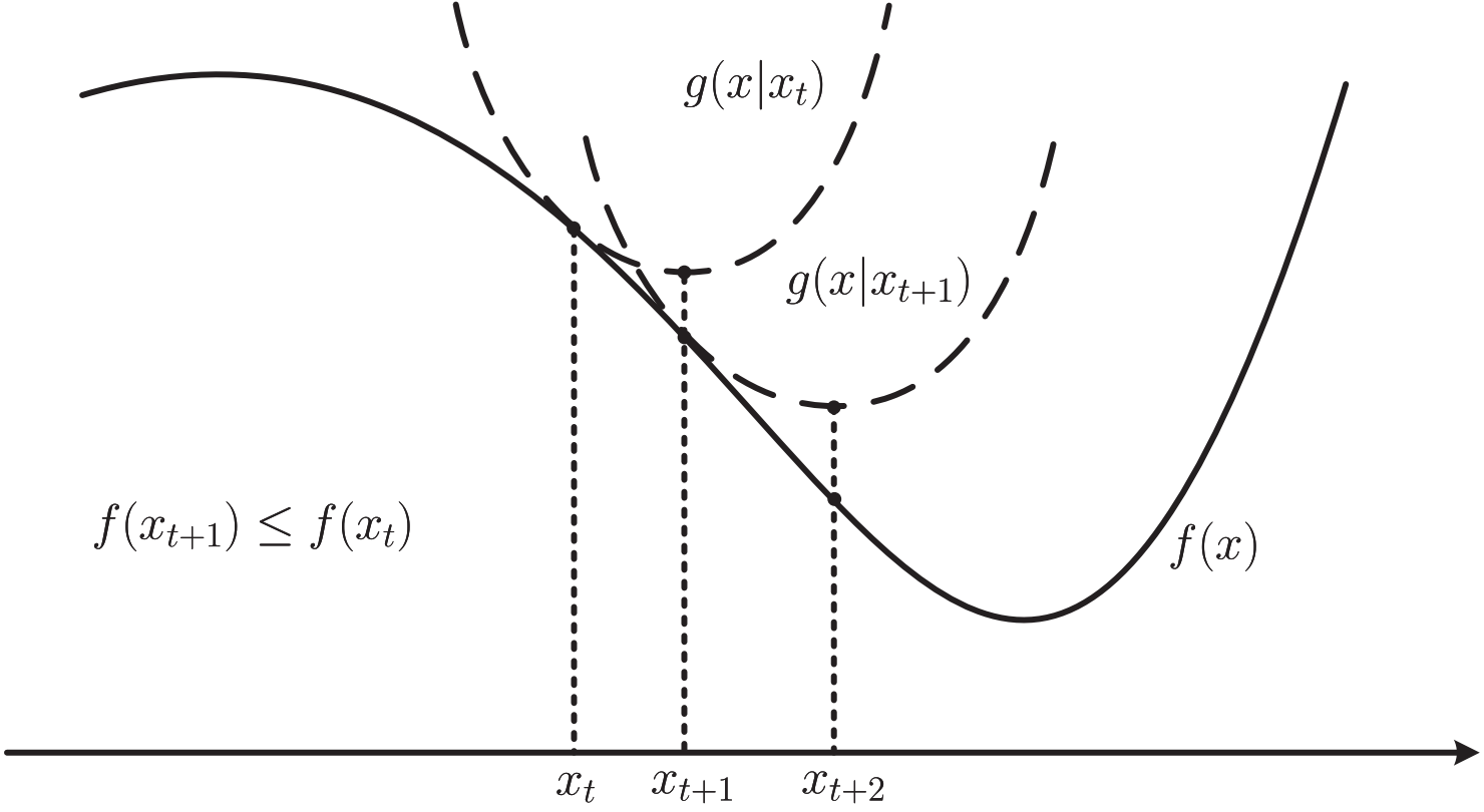
Figure 3: The MM procedure [15].

The MM algorithm is described in figure 3. The key feature of the MM algorithm is that at each iteration it decreases the objective function monotonically

$$f\left(\mathbf{x}_{t+1}\right)\leq g\left(\mathbf{x}_{t+1}\mid\mathbf{x}_{t}\right)\leq g\left(\mathbf{x}_{t}\mid\mathbf{x}_{t}\right)=f\left(\mathbf{x}_{t}\right).$$ (22)

The first inequality from the right side follows from the definition of $\mathbf{x}_{t+1}$ in (21) and second inequality follows from (20).

III-B MM over Primal and Dual Variables

In the proposed algorithm, we are utilizing the MM algorithm and the duality principle from the optimization theory to solve the problem in (13). The problem in (13) is the original optimization problem which we want to solve. We solve this problem with MM algorithm, iteratively. Each iteration of the MM algorithm involves two steps: majorization and minimization. In the majorization step, we form the surrogate function for the objective function of the original problem (13) which majorizes the objective function. In the minimization step, instead of minimizing the surrogate function, we form the dual problem for the problem of minimizing the surrogate function, and solve the dual problem using the MM algorithm. Sometimes after the majorization or minorization step, the surrogate function which we get is not easy to solve or the surrogate function can’t be solved iteratively via the MM algorithm. In such cases, we make the dual problem for the minimization problem of the surrogate function and solve the dual problem over dual variable by MM algorithm. If strong duality holds then from the dual optimal solution we can find the primal optimal solution. Therefore, we call this proposed algorithm as MM over primal dual variable. Figure 4 shows the flowchart for the proposed algorithm. Now we develop the idea of MM over primal dual variables for the problem (13).

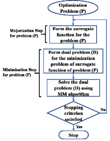
Figure 4: Flowchart for MM over primal dual variables.

The optimization problem (13) is

$$\underset{\mathbf{H}}{\text{minimize}} f_{0}\left(\mathbf{H}\right)\triangleq\mathrm{Tr}\left(\left(\mathbf{H}^{T}\mathbf{R}^{-1}\mathbf{H}\right)^{-1}\right)$$ (23)

subject to $$\mathbf{h}_{i}^{T}\mathbf{h}_{i}=1,\;i=1,\ldots,m$$

where $f_{0}\left(\mathbf{H}\right)$ is the objective function, $\mathbf{H}\in\mathbb{R}^{m\times n}$ is variable, $\mathbf{R}\in\mathbb{S}_{m}^{+}$ is measurement noise covariance matrix and $\mathbf{h}_{i}^{T}$ is the $i^{th}$ row of $\mathbf{H}$. Let $D_{f_{0}}$ be the domain of the optimization problem (23) then we can write $D_{f_{0}}$ as

$$D_{f_{0}}=\left\{\mathbf{H}\in\mathbb{R}^{m\times n}\mid\mathbf{h}_{i}^{T}\mathbf{h}_{i}=1,\;i=1,\ldots,m\right\}$$ (24)

The epigraph form for the problem (23) is

$$\underset{\mathbf{\mathbf{H}}\in D_{f_{0}},a_{1},\ldots,a_{n}}{\text{minimize}} \sum_{k=1}^{n}a_{k}$$ (25)

subject to $$\left[\begin{array}[]{cc}a_{k}&\mathbf{e}_{k}^{T}\\ \mathbf{e}_{k}&\mathbf{H}^{T}\mathbf{R}^{-1}\mathbf{H}\end{array}\right]\succeq 0,$$

$$k=1,\ldots,n$$

where $\mathbf{e}_{k}$ is the $k^{th}$ column of the $n\times n$ identity matrix $\mathbf{I}_{n}$.

Reformulating problem (25) we get:

$$\begin{aligned} &\underset{\mathbf{\mathbf{H}}\in D_{f_{0}},a_{1},\ldots,a_{n}}{\text{minimize}}&&\sum_{k=1}^{n}a_{k}\\ &\text{subject to}&&\mathbf{H}^{T}\mathbf{R}^{-1}\mathbf{H}\succ 0\\ &&&a_{k}-\mathbf{e}_{k}^{T}\left(\mathbf{H}^{T}\mathbf{R}^{-1}\mathbf{H}\right)^{-1}\mathbf{e}_{k}\succeq 0,\\ &&&k=1,\ldots,n\end{aligned}.$$ (26)

Next we discuss briefly about the difference of convex (DC) programming. In fact, the DC programming can be shown to be a special case of MM algorithm. In DC programming, difference of convex function is minimized with constraints being also the difference of convex functions. The DC programming can also be seen as the minimization of the sum of a convex and a concave function with constraints being the sum of convex and concave functions. The DC programming is not a convex problem but it can be converted to a convex programming problem by replacing the concave functions in the objective function and the constraints by its first order Taylor approximation at current iteration point [17]. With this substitution the DC programming becomes a convex problem and can be solved via standard tool [18]. Similar approach can be adopted for the problem (26) in which we replace $\mathbf{H}^{T}\mathbf{R}^{-1}\mathbf{H}$ by $\boldsymbol{\Phi}\left(\mathbf{H};\mathbf{H}_{t}\right)\triangleq-\mathbf{H}_{t}^{T}\mathbf{R}^{-1}\mathbf{H}_{t}+\mathbf{H}^{T}\mathbf{R}^{-1}\mathbf{H}_{t}+\mathbf{H}_{t}^{T}\mathbf{R}^{-1}\mathbf{H}$, its first order Taylor approximation at $\mathbf{H}_{t}$. With this subsitution in problem (26) we get:

$$\underset{\mathbf{\mathbf{H}}\in D_{f_{0}},a_{1},\ldots,a_{n}}{\text{minimize}} \sum_{k=1}^{n}a_{k}$$ (27)

subject to $$\boldsymbol{\Phi}\left(\mathbf{H};\mathbf{H}_{t}\right)\succ 0$$

$$a_{k}-\mathbf{e}_{k}^{T}\left(\boldsymbol{\Phi}\left(\mathbf{H};\mathbf{H}_{t}\right)\right)^{-1}\mathbf{e}_{k}\succeq 0,$$

$$k=1,\ldots,n$$

If we undo the epigraph form for problem (27) we get:

$$\underset{\mathbf{\mathbf{H}}\in D_{f_{0}}}{\text{minimize}} \mathrm{Tr}\left(\left(\boldsymbol{\Phi}\left(\mathbf{H};\mathbf{H}_{t}\right)\right)^{-1}\right)$$ (28)

subject to $$\boldsymbol{\Phi}\left(\mathbf{H};\mathbf{H}_{t}\right)\succ 0$$

The objective function of the problem (28) is the surrogate function for $f_{0}\left(\mathbf{H}\right)$ which upperbounds it. We Denote the objective function of problem (28) by:

$$g_{f_{0}}\left(\mathbf{H}\mid\mathbf{H}_{t}\right)\triangleq\mathrm{Tr}\left(\left(\boldsymbol{\Phi}\left(\mathbf{H};\mathbf{H}_{t}\right)\right)^{-1}\right).$$ (29)

The surrogate function $g_{f_{0}}\left(\mathbf{H}\mid\mathbf{H}_{t}\right)$ satisfies the following property:

$$f_{0}\left(\mathbf{\mathbf{H}_{t}}\right)=g_{f_{0}}\left(\mathbf{H}_{t}\mid\mathbf{H}_{t}\right)$$ (30)

$$f_{0}\left(\mathbf{H}\right)\leq g_{f_{0}}\left(\mathbf{H}\mid\mathbf{H}_{t}\right) \textrm{if}\>\boldsymbol{\Phi}\left(\mathbf{H};\mathbf{H}_{t}\right)\succ 0$$

Reformulating the problem (27) we get:

$$\underset{\mathbf{\mathbf{H}}\in D_{f_{0}},a_{1},\ldots,a_{n}}{\text{minimize}} \sum_{k=1}^{n}a_{k}$$ (31)

subject to $$\left[\begin{array}[]{cc}a_{k}&\mathbf{e}_{k}^{T}\\ \mathbf{e}_{k}&\boldsymbol{\Phi}\left(\mathbf{H};\mathbf{H}_{t}\right)\end{array}\right]\succeq 0.$$

$$k=1,\ldots,n$$

We can relax the constraint $\mathbf{\mathbf{H}}\in D_{f_{0}}$ in problem (31) to make this problem a semidefinite programming (SDP). We define the following relaxed constraint:

$$D=\left\{\mathbf{H}\in\mathbb{R}^{m\times n}\mid\mathbf{h}_{i}^{T}\mathbf{h}_{i}\leq 1,\;i=1,\ldots,m\right\}.$$ (32)

If we now let $\mathbf{\mathbf{H}}\in D$ in problem (31), it becomes SDP. This relaxation does not affect the optimal solution of the problem (31) because the objective function in problem (31) is linear and a linear objective function achieves its optimal solution at the boundary of the constraint. After relaxing the constraint $\mathbf{\mathbf{H}}\in D_{f_{0}}$ by $\mathbf{\mathbf{H}}\in D$ in problem (31), we get the following SDP:

$$\underset{\mathbf{\mathbf{H}}\in D,a_{1},\ldots,a_{n}}{\text{minimize}} \sum_{k=1}^{n}a_{k}$$ (33)

subject to $$\left[\begin{array}[]{cc}a_{k}&\mathbf{e}_{k}^{T}\\ \mathbf{e}_{k}&\boldsymbol{\Phi}\left(\mathbf{H};\mathbf{H}_{t}\right)\end{array}\right]\succeq 0,$$

$$k=1,\ldots,n$$

At the optimal solution of the problem (33) the constraint $\mathbf{\mathbf{H}}\in D$ will be tight. The problem in (33) is SDP and can be solved to find the next update of the variable $\mathbf{\mathbf{H}}$ $i.e.$ $\mathbf{H}_{t+1}$. Solving this SDP may have some issues: we may have to rely on solver, complexity of the problem increases when the dimension of the variable $\mathbf{\mathbf{H}}$ increases, for higer dimension of $\mathbf{\mathbf{H}}$, solvers may take long time and memory issue may also result. Therefore, directly solving the SDP in (33) is not recommended. So we form the dual problem for SDP in (33) and see if the dual problem can be solved easily and efficiently. As we progress further we will see that using the proposed algorithm obviates the need of any solver.

Next we form the Lagrangian for problem (33). Let $\mathbf{G}_{k}=\left(\begin{array}[]{cc}p_{k}&\mathbf{q}_{k}^{T}\\ \mathbf{q}_{k}&\mathbf{S}_{k}\end{array}\right)$ be the Lagrange multiplier for each semidefinite constraint. Then we can write the Lagrangian as

$$\begin{array}[]{c}L\left(\mathbf{H},a_{1},\ldots,a_{n},\mathbf{G}_{1},\ldots,\mathbf{G}_{n}\right)=\sum_{k=1}^{n}a_{k}-\\ \sum_{k=1}^{n}\mathrm{Tr}\left(\mathbf{G}_{k}\left(\begin{array}[]{cc}a_{k}&\mathbf{e}_{k}^{T}\\ \mathbf{e}_{k}&\boldsymbol{\Phi}\left(\mathbf{H};\mathbf{H}_{t}\right)\end{array}\right)\right)\end{array}$$ (34)

With some manipulations, we can write the equation (34) as

$$\begin{array}[]{c}L\left(\mathbf{H},a_{1},\ldots,a_{n},\mathbf{G}_{1},\ldots,\mathbf{G}_{n}\right)=\sum_{k=1}^{n}\left(1-p_{k}\right)a_{k}-\\ 2\mathrm{Tr}\left(\mathbf{R}^{-1}\mathbf{H}_{t}\mathbf{S}\mathbf{H}^{T}\right)+\sum_{k=1}^{n}\mathrm{Tr}\left(\mathbf{G}_{k}\mathbf{D}_{k}\right)\end{array}$$ (35)

where $\mathbf{D}_{k}=\left(\begin{array}[]{cc}0&-\mathbf{e}_{k}^{T}\\ -\mathbf{e}_{k}&\mathbf{H}_{t}^{T}\mathbf{R}^{-1}\mathbf{H}_{t}\end{array}\right)$and $\mathbf{S}=\sum_{k=1}^{n}\mathbf{S}_{k}$.

Now we find the Lagrange dual function. The Lagrange dual function is defined as the infimum of the Lagrangian over primal variables. The dual function is concave function of the Lagrange multipliers (also called the dual variables) irrespective of the primal problem is convex or not [14]. So the dual function is given by

$$g\left(\mathbf{G}_{1},\ldots,\mathbf{G}_{n}\right)=\underset{\mathbf{\mathbf{H}}\in D_{f_{0}},a_{1},\ldots,a_{n}}{\text{inf}}L\left(\mathbf{H},a_{1},\ldots,a,\mathbf{G}_{1},\ldots,\mathbf{G}_{n}\right)$$ (36)

The Lagrangian in (35) is bounded below in $a_{k}$ if $p_{k}=1$, so the dual function becomes

$$g\left(\mathbf{G}_{1},\ldots,\mathbf{G}_{n}\right)=\sum_{k=1}^{n}\mathrm{Tr}\left(\mathbf{G}_{k}\mathbf{D}_{k}\right)+\underset{\mathbf{\mathbf{H}}\in D_{f_{0}}}{\text{inf}}-2\mathrm{Tr}\left(\mathbf{R}^{-1}\mathbf{H}_{t}\mathbf{S}\mathbf{H}^{T}\right)$$ (37)

Assuming $\mathbf{R}^{-1}\mathbf{H}_{t}=\mathbf{C}_{t}=\left(\begin{array}[]{c}\left(\widetilde{\mathbf{c}}_{1}^{t}\right)^{T}\\ \vdots\\ \left(\widetilde{\mathbf{c}}_{m}^{t}\right)^{T}\end{array}\right)$, we have

$$g\left(\mathbf{G}_{1},\ldots,\mathbf{G}_{n}\right)=\sum_{k=1}^{n}\mathrm{Tr}\left(\mathbf{G}_{k}\mathbf{D}_{k}\right)-2\underset{\mathbf{\mathbf{H}}\in D_{f_{0}}}{\text{sup}}\mathrm{Tr}\left(\mathbf{C}_{t}\mathbf{S}\mathbf{H}^{T}\right)$$ (38)

Lemma 1.

Given $\mathbf{b}\in\mathbb{R}^{n}$, $\underset{\mathbf{x}^{T}\mathbf{x}=1}{\text{sup}}\mathbf{b}^{T}\mathbf{x}=\left\|\mathbf{b}\right\|_{2}$ and occurs at $\mathbf{x}=\frac{\mathbf{b}}{\left\|\mathbf{b}\right\|_{2}}$.

Now the supremum of the second term in (38), using the lemma 1 is given by

$$\underset{\mathbf{\mathbf{H}}\in D_{f_{0}}}{\text{sup}}\mathrm{Tr}\left(\mathbf{C}_{t}\mathbf{S}\mathbf{H}^{T}\right)=\sum_{i=1}^{m}\left\|\mathbf{S}\widetilde{\mathbf{c}}_{i}^{t}\right\|_{2}$$ (39)

and this supremum occurs at

$$\mathbf{h}_{i}=\frac{\mathbf{S}\widetilde{\mathbf{c}}_{i}^{t}}{\left\|\mathbf{S}\widetilde{\mathbf{c}}_{i}^{t}\right\|_{2}}.$$ (40)

so we have the following dual function:

$$g\left(\mathbf{G}_{1},\ldots,\mathbf{G}_{n}\right)=\sum_{k=1}^{n}\mathrm{Tr}\left(\mathbf{G}_{k}\mathbf{D}_{k}\right)-2\sum_{i=1}^{m}\left\|\mathbf{S}\widetilde{\mathbf{c}}_{i}^{t}\right\|_{2}$$ (41)

so the dual problem of the problem (33) is

$$\underset{}{\text{maximize}} \sum_{k=1}^{n}\mathrm{Tr}\left(\left(\begin{array}[]{cc}1&\mathbf{q}_{k}^{T}\\ \mathbf{q}_{k}&\mathbf{S}_{k}\end{array}\right)\mathbf{D}_{k}\right)-2\sum_{i=1}^{m}\left\|\mathbf{S}\widetilde{\mathbf{c}}_{i}^{t}\right\|_{2}$$ (42)

subject to $$\left(\begin{array}[]{cc}1&\mathbf{q}_{k}^{T}\\ \mathbf{q}_{k}&\mathbf{S}_{k}\end{array}\right)\succeq 0,\;k=1,\ldots,n$$

$$\mathbf{S}=\sum_{k=1}^{n}\mathbf{S}_{k}$$

Since the problem (33) is convex, strong duality holds, that is, optimal value of problem (33) equals the optimal value of the problem (42).

Reformulating (42) we get,

$$\underset{}{\text{minimize}} 2\sum_{i=1}^{m}\left\|\mathbf{S}\widetilde{\mathbf{c}}_{i}^{t}\right\|_{2}-\sum_{k=1}^{n}\mathrm{Tr}\left(\left(\begin{array}[]{cc}1&\mathbf{q}_{k}^{T}\\ \mathbf{q}_{k}&\mathbf{S}_{k}\end{array}\right)\mathbf{D}_{k}\right)$$ (43)

subject to $$\left(\begin{array}[]{cc}1&\mathbf{q}_{k}^{T}\\ \mathbf{q}_{k}&\mathbf{S}_{k}\end{array}\right)\succeq 0,\;k=1,\ldots,n$$

$$\mathbf{S}=\sum_{k=1}^{n}\mathbf{S}_{k}$$

The dual problem of the problem (33) is also SDP and at the optimal solution of the problem (43) the linear matrix inequality will be tight, that is, $\mathbf{S}_{k}=\mathbf{q}_{k}\mathbf{q}_{k}^{T}$ for $k=1,\ldots,n$. Solving the dual SDP in (43) is also not cheap so we will solve this dual SDP using MM algorithm. Substituting $\mathbf{S}_{k}=\mathbf{q}_{k}\mathbf{q}_{k}^{T}$ in problem (43) we have $\mathbf{S}=\sum_{k=1}^{n}\mathbf{S}_{k}=\sum_{k=1}^{n}\mathbf{q}_{k}\mathbf{q}_{k}^{T}=\mathbf{Q}\mathbf{Q}^{T}$ where $\mathbf{Q}=\left(\begin{array}[]{ccc}\mathbf{q}_{1}&\ldots&\mathbf{q}_{n}\end{array}\right)$, and the following unconstrained optimization problem is achieved:

$$\underset{\mathbf{Q}}{\text{minimize}}\;2\sum_{i=1}^{m}\left\|\mathbf{Q}\mathbf{Q}^{T}\widetilde{\mathbf{c}}_{i}^{t}\right\|_{2}+\mathrm{Tr}\left(2\mathbf{Q}^{T}-\mathbf{Q}^{T}\mathbf{H}_{t}^{T}\mathbf{R}^{-1}\mathbf{H}_{t}\mathbf{Q}\right)$$ (44)

and the objective function is denoted by $\gamma\left(\mathbf{Q}\right)\triangleq 2\sum_{i=1}^{m}\left\|\mathbf{Q}\mathbf{Q}^{T}\widetilde{\mathbf{c}}_{i}^{t}\right\|_{2}+\mathrm{Tr}\left(2\mathbf{Q}^{T}-\mathbf{Q}^{T}\mathbf{H}_{t}^{T}\mathbf{R}^{-1}\mathbf{H}_{t}\mathbf{Q}\right)$.

Reformulating problem (44), we have the following:

$$\underset{\mathbf{Q},\beta_{1},\ldots,\beta_{m}}{\text{minimize}} 2\sum_{i=1}^{m}\sqrt{\beta_{i}}+\mathrm{Tr}\left(2\mathbf{Q}^{T}-\mathbf{Q}^{T}\mathbf{H}_{t}^{T}\mathbf{R}^{-1}\mathbf{H}_{t}\mathbf{Q}\right)$$ (45)

subject to $$\beta_{i}=\left\|\mathbf{Q}\mathbf{Q}^{T}\widetilde{\mathbf{c}}_{i}^{t}\right\|_{2}^{2},\;i=1,\ldots,m.$$

Denote the objective function of the problem (45) by $\psi\left(\mathbf{Q},\boldsymbol{\beta}\right)\triangleq 2\sum_{i=1}^{m}\sqrt{\beta_{i}}+\mathrm{Tr}\left(2\mathbf{Q}^{T}-\mathbf{Q}^{T}\mathbf{H}_{t}^{T}\mathbf{R}^{-1}\mathbf{H}_{t}\mathbf{Q}\right)$, where $\boldsymbol{\beta}=\left(\begin{array}[]{ccc}\beta_{1}&\ldots&\beta_{m}\end{array}\right)^{T}$, $\psi_{1}\left(\boldsymbol{\beta}\right)\triangleq 2\sum_{i=1}^{m}\sqrt{\beta_{i}}$, and $\psi_{2}\left(\mathbf{Q}\right)\triangleq\mathrm{Tr}\left(2\mathbf{Q}^{T}-\mathbf{Q}^{T}\mathbf{H}_{t}^{T}\mathbf{R}^{-1}\mathbf{H}_{t}\mathbf{Q}\right)$. Therefore, $\psi\left(\mathbf{Q},\boldsymbol{\beta}\right)=\psi_{1}\left(\boldsymbol{\beta}\right)+\psi_{2}\left(\mathbf{Q}\right)$.

Lemma 2.

Given $\beta_{i}^{\tau}$, the function $\sqrt{\beta_{i}}$ can be upperbounded as

$$\sqrt{\beta_{i}}\leq\sqrt{\beta_{i}^{\tau}}+\frac{1}{2\sqrt{\beta_{i}^{\tau}}}\left(\beta_{i}-\beta_{i}^{\tau}\right)$$ (46)

with equality achieved at $\beta_{i}=\beta_{i}^{\tau}$.

Proof:

The proof is obvious when we write the first order Taylor expansion for the function $\sqrt{\beta_{i}}$ at $\beta_{i}^{\tau}$. ∎

Lemma 3.

Given $\mathbf{Q}_{\tau}$, the function $w\left(\mathbf{Q}\right)\triangleq\mathrm{Tr}\left(\mathbf{B}\mathbf{Q}^{T}-\mathbf{Q}^{T}\mathbf{A}\mathbf{Q}\right)$, with $\mathbf{A}\in\mathbb{S}_{+}^{n}$, $\mathbf{B}\in\mathbb{R}^{n\times n}$, and $\mathbf{Q}\in\mathbb{R}^{n\times n}$, can be upperbounded as

$$w\left(\mathbf{Q}\right)\leq w\left(\mathbf{Q}_{\tau}\right)+\mathrm{Tr}\left(\left(\mathbf{B}^{T}-2\mathbf{Q}_{\tau}^{T}\mathbf{A}\right)\left(\mathbf{Q}-\mathbf{Q}_{\tau}\right)\right)$$ (47)

with equality achieved at $\mathbf{Q}=\mathbf{Q}_{\tau}$.

Proof:

Writing the first order Taylor expansion for $w\left(\mathbf{Q}\right)$ at $\mathbf{Q}_{\tau}$, we get the above mentioned result. ∎

Using lemma 2, $\psi_{1}\left(\boldsymbol{\beta}\right)$ can be upperbounded at $\boldsymbol{\beta}^{\tau}$ as:

$$\psi_{1}\left(\boldsymbol{\beta}\right)\leq g_{\psi_{1}}\left(\boldsymbol{\beta}\mid\boldsymbol{\beta}^{\tau}\right),$$ (48)

where $g_{\psi_{1}}\left(\boldsymbol{\beta}\mid\boldsymbol{\beta}^{\tau}\right)\triangleq\sum_{i=1}^{m}\left(\sqrt{\beta_{i}^{\tau}}+\frac{1}{2\sqrt{\beta_{i}^{\tau}}}\left(\beta_{i}-\beta_{i}^{\tau}\right)\right)$.

The function $\psi_{2}\left(\mathbf{Q}\right)$ can be upperbounded using lemma 3 as:

$$\psi_{2}\left(\mathbf{Q}\right)\leq g_{\psi_{2}}\left(\mathbf{Q}\mid\mathbf{Q}_{\tau}\right),$$ (49)

where $g_{\psi_{2}}\left(\mathbf{Q}\mid\mathbf{Q}_{\tau}\right)\triangleq\psi_{2}\left(\mathbf{Q}_{\tau}\right)+2\mathrm{Tr}\left(\mathbf{P}_{t,\tau}\left(\mathbf{Q}-\mathbf{Q}_{\tau}\right)\right)$, and

$$\mathbf{P}_{t,\tau}=\mathbf{I}_{n}-\mathbf{Q}_{\tau}^{T}\mathbf{H}_{t}^{T}\mathbf{R}^{-1}\mathbf{H}_{t}.$$ (50)

Therefore the surrogate function which upperbounds the $\psi\left(\mathbf{Q},\boldsymbol{\beta}\right)$ can be written as:

$$\psi\left(\mathbf{Q},\boldsymbol{\beta}\right)\leq g_{\psi}\left(\mathbf{Q},\boldsymbol{\beta}\mid\mathbf{Q}_{\tau},\boldsymbol{\beta}^{\tau}\right),$$ (51)

where $g_{\psi}\left(\mathbf{Q},\boldsymbol{\beta}\mid\mathbf{Q}_{\tau},\boldsymbol{\beta}^{\tau}\right)=g_{\psi_{1}}\left(\boldsymbol{\beta}\mid\boldsymbol{\beta}^{\tau}\right)+g_{\psi_{2}}\left(\mathbf{Q}\mid\mathbf{Q}_{\tau}\right)$.

Since $\gamma\left(\mathbf{Q}\right)=\psi\left(\mathbf{Q},\boldsymbol{\beta}\right)$ with $\beta_{i}=\left\|\mathbf{Q}\mathbf{Q}^{T}\widetilde{\mathbf{c}}_{i}^{t}\right\|_{2}^{2}$ for $i=1,\ldots,m$, the surrogate function $g_{\gamma}\left(\mathbf{Q}\mid\mathbf{Q}_{\tau}\right)$ which upperbounds the $\gamma\left(\mathbf{Q}\right)$ at $\mathbf{Q}_{\tau}$ can be written as:

$$g_{\gamma}\left(\mathbf{Q}\mid\mathbf{Q}_{\tau}\right)=g_{\psi}\left(\mathbf{Q},\boldsymbol{\beta}\mid\mathbf{Q}_{\tau},\boldsymbol{\beta}^{\tau}\right)\,\text{with}\,\beta_{i}=\left\|\mathbf{Q}\mathbf{Q}^{T}\widetilde{\mathbf{c}}_{i}^{t}\right\|_{2}^{2}$$ (52)

The surrogate function in (52) satisfies:

$$\begin{aligned} \gamma\left(\mathbf{\mathbf{Q}_{\tau}}\right)=g_{\gamma}\left(\mathbf{Q}_{\tau}\mid\mathbf{Q}_{\tau}\right)\\ \gamma\left(\mathbf{Q}\right)\leq g_{\gamma}\left(\mathbf{Q}\mid\mathbf{Q}_{\tau}\right)\end{aligned}.$$ (53)

Now we solve the problem (45) iteratively using the MM algorithm. Minimizing the surrogate function $g_{\gamma}\left(\mathbf{Q}\mid\mathbf{Q}_{\tau}\right)$ with respect to $\mathbf{Q}$ gives the next iteration point $\mathbf{Q}_{\tau+1}$.

$$\mathbf{Q}_{\tau+1}= \text{arg }\underset{\mathbf{Q}}{\text{min}}\>g_{\gamma}\left(\mathbf{Q}\mid\mathbf{Q}_{\tau}\right)$$ (54)

Leaving the constant terms in $g_{\gamma}\left(\mathbf{Q}\mid\mathbf{Q}_{\tau}\right)$ the problem (54) can be written as:

$$\mathbf{Q}_{\tau+1}=\text{arg }\underset{\mathbf{Q}}{\text{min}}\left(\sum_{i=1}^{m}\frac{\left\|\mathbf{Q}\mathbf{Q}^{T}\widetilde{\mathbf{c}}_{i}^{t}\right\|_{2}^{2}}{\left\|\mathbf{Q}_{\tau}\mathbf{Q}_{\tau}^{T}\widetilde{\mathbf{c}}_{i}^{t}\right\|_{2}}+2\mathrm{Tr}\left(\mathbf{Q}\mathbf{P}_{t,\tau}\right)\right).$$ (55)

Problem (55) can be rewritten as

$$\mathbf{Q}_{\tau+1}=\text{arg }\underset{\mathbf{Q}}{\text{min}}\left(\mathrm{Tr}\left(\mathbf{F}_{t,\tau}\mathbf{Q}\mathbf{Q}^{T}\mathbf{Q}\mathbf{Q}^{T}\right)+2\mathrm{Tr}\left(\mathbf{Q}\mathbf{P}_{t,\tau}\right)\right)$$ (56)

where

$$\mathbf{F}_{t,\tau}=\mathbf{C}_{t}^{T}\mathbf{U}_{t,\tau}\mathbf{C}_{t}$$ (57)

with $\mathbf{U}_{t,\tau}=\left(\begin{array}[]{ccc}u_{11}^{t,\tau}\\ &\ddots\\ &&u_{mm}^{t,\tau}\end{array}\right)$ and each $u_{ii}^{t,\tau}=\frac{1}{\left\|\mathbf{Q}_{\tau}\mathbf{Q}_{\tau}^{T}\widetilde{\mathbf{c}}_{i}^{t}\right\|_{2}}$.

Since no closed form solution available for problem (56) we resort to coordinate descent method to minimize the problem (56) and find the next iteration point $\mathbf{Q}_{\tau+1}$. In the coordinate descent method, we minimize the objective function iteratively with respect to the one variable while keeping the rest of the variables fixed. Let $\mathbf{Q}_{\tau}$ be the value of the variable $\mathbf{Q}$ at $\tau-$th iteration. To do the coordinate descent with respect to $q_{ij}$, where $q_{ij}$ is the $\left(i,j\right)$ element of the variable $\mathbf{Q}$, we put $q_{ij}\mathbf{e}_{i}\mathbf{e}_{j}^{T}+\mathbf{Q}_{\tau}^{ij}$ in place of $\mathbf{Q}$ in (56) and obtain the quartic polynomial in $q_{ij}$. Here $\mathbf{e}_{i}$ denotes the $i^{th}$ column of the $n\times n$ identity matrix $\mathbf{I}_{n}$ and $\mathbf{Q}_{\tau}^{ij}$ denotes the $\tau-$th iteration point with its $\left(i,j\right)$ element equal to zero. The quartic polynomial in $q_{ij}$ is given by

$$r\left(q_{ij}\right)=aq_{ij}^{4}+bq_{ij}^{3}+cq_{ij}^{2}+dq_{ij}+e$$ (58)

The coefficients of polynomial (58) can be computed using following relations:

$$a= \mathrm{Tr}\left(\mathbf{F}_{t,\tau}\mathbf{K}_{ij}\right)$$ (59)

$$b= \mathrm{Tr}\left(\mathbf{F}_{t,\tau}\left(\mathbf{K}_{ij}\mathbf{L}_{ij}+\mathbf{L}_{ij}\mathbf{K}_{ij}\right)\right)$$

$$c= \mathrm{Tr}\left(\mathbf{F}_{t,\tau}\left(\mathbf{M}_{ij}\mathbf{K}_{ij}+\mathbf{L}_{ij}^{2}+\mathbf{K}_{ij}\mathbf{M}_{ij}\right)\right)$$

$$d= \mathrm{Tr}\left(\mathbf{F}_{t,\tau}\left(\mathbf{M}_{ij}\mathbf{L}_{ij}+\mathbf{L}_{ij}\mathbf{M}_{ij}\right)\right)+2\mathrm{Tr}\left(\mathbf{E}_{ij}\mathbf{P}_{t,\tau}\right)$$

$$e= \mathrm{Tr}\left(\mathbf{F}_{t,\tau}\mathbf{M}_{ij}^{2}\right)+2\mathrm{Tr}\left(\mathbf{Q}_{\tau}^{ij}\mathbf{P}_{t,\tau}\right)$$

where $\mathbf{E}_{ij}=\mathbf{e}_{i}\mathbf{e}_{j}^{T}$, $\mathbf{E}_{ji}=\mathbf{E}_{ij}^{T}$, $\mathbf{K}_{ij}=\mathbf{E}_{ij}\mathbf{E}_{ji}$, $\mathbf{L}_{ij}=\mathbf{Q}_{\tau}^{ij}\mathbf{E}_{ji}+\mathbf{E}_{ij}\left(\mathbf{Q}_{\tau}^{ij}\right)^{T}$and $\mathbf{M}_{ij}=\mathbf{Q}_{\tau}^{ij}\left(\mathbf{Q}_{\tau}^{ij}\right)^{T}$.

The reason for using the coordinate descent method is that the dimension of the $\mathbf{Q}$ is $n\times n$, that is, $3\times 3$ so we have only nine variables for which we have to do the coordinate descent and this remains fixed irrespective of the number of sensors $m$. For this reason the coordinate descent method is preferred here.

Each $q_{ij}$ is updated as follows:

$$q_{ij}^{\tau+1}=\text{arg }\underset{q_{ij}}{\text{min}}\>r\left(q_{ij}\right)$$ (60)

When the coordinate descent for all $q_{ij}$ is completed we get the next iteration point $\mathbf{Q}_{\tau+1}$. The coordinate descent method is repeated many times until we get the minimum for the problem (44). Let $\mathbf{Q}_{*}$ be the optimal solution of the problem (44) obtained after $N$ cycle of the coordinate descent then $\mathbf{Q}_{*}=\mathbf{Q}_{\tau+N}$. After this we compute the next update of the variable $\mathbf{H}$ $i.e$ $\mathbf{H}_{t+1}$. From optimal solution $\mathbf{Q}_{*}$, we compute optimal $\mathbf{S}$ using $\mathbf{S}_{*}=\mathbf{Q}_{*}\mathbf{Q}_{*}^{T}$.

The $\mathbf{H}_{t}$ is updated to $\mathbf{H}_{t+1}$ by using following relations:

$$\mathbf{h}_{i}^{t+1}=\frac{\mathbf{S}_{*}\widetilde{\mathbf{c}}_{i}^{t}}{\left\|\mathbf{S}_{*}\widetilde{\mathbf{c}}_{i}^{t}\right\|_{2}},$$ (61)

and

$$\mathbf{H}_{t+1}=\left(\begin{array}[]{c}\left(\mathbf{h}_{1}^{t+1}\right)^{T}\\ \vdots\\ \left(\mathbf{h}_{m}^{t+1}\right)^{T}\end{array}\right).$$ (62)

After obtaining the next iteration $\mathbf{H}_{t+1}$ we repeat the algorithm multiple times to obtain the optimal solution for the problem (23). Suppose the optimal $\mathbf{H}$ is achieved after $M$ iteration then $\mathbf{H}_{*}=\mathbf{H}_{t+M}$. The single iteration of the proposed algorithm is as shown in figure 5. The steps of the proposed primal dual MM algorithm is described in algorithm 1.

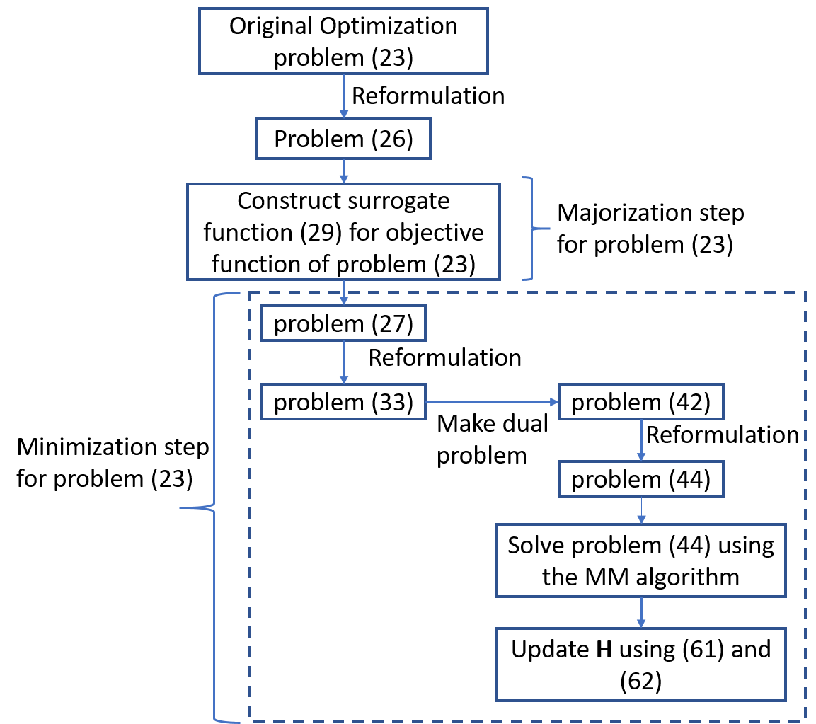
Figure 5: Single iteration of the proposed algorithm for problem (13).

  Initialize $\mathbf{H}_{0}\in D_{f_{0}}$.

  Set $t$, $\tau=0$.Repeat:

   Initialize $\mathbf{Q}_{0}\in\mathbb{R}^{n\times n}$.  Repeat:   Compute $\mathbf{P}_{t,\tau}$ and $\mathbf{F}_{t,\tau}$ given in (50) and (57) respectively.  $\mathbf{Q}_{\tau+1}=\mathbf{Q}_{\tau}$   for $i=1,\ldots,n$    for $j=1,\ldots,n$

      Compute $a$, $b$, $c$, $d$ and $e$, the coefficients of the quartic polynomial $r\left(q_{ij}\right)$ in (58) using (59).

      $q_{ij}^{\tau+1}=\text{arg}\,\underset{q_{ij}}{\text{min}\>}r\left(q_{ij}\right)$

      $\mathbf{Q}_{\tau+1}\left(i,j\right)=q_{ij}^{\tau+1}$    end   end  $\tau\leftarrow\tau+1$  until convergence

  Compute $\mathbf{S}_{*}=\mathbf{Q}_{*}\mathbf{Q}_{*}^{T}$, where $\mathbf{Q}_{*}$ is the value of $\mathbf{Q}_{\tau}$ after convergence.

  Compute $\mathbf{h}_{i}^{t+1}=\frac{\mathbf{S}_{*}\widetilde{\mathbf{c}}_{i}^{t}}{\left\|\mathbf{S}_{*}\widetilde{\mathbf{c}}_{i}^{t}\right\|_{2}}$ for $i=1,\ldots,m$ and form the $\mathbf{H}_{t+1}$ as described in (62).

  $t\leftarrow t+1$ until convergence

  output: $\mathbf{H}_{*}$, where $\mathbf{H}_{*}$ is the value of $\mathbf{H}_{t}$ after convergence.

Algorithm 1 MM algorithm over primal and dual variables.

III-C Solving D-optimal Problem by the Proposed Algorithm

In this section, we solve the problem described in (11) using the proposed algorithm. The problem (11) can be reformulated as

$$\underset{\mathbf{H},\mathbf{W},\mathbf{B}}{\text{minimize}} \log\det\left(\mathbf{B}\right)$$ (63)

subject to $$\mathbf{h}_{i}^{T}\mathbf{h}_{i}=1,\;i=1,\ldots,m$$

$$\mathbf{W}=\mathbf{H}^{T}\mathbf{R}^{-1}\mathbf{H}$$

$$\mathbf{B}=\mathbf{W}^{-1}$$

The objective function $f\left(\mathbf{B}\right)\triangleq\log\det\left(\mathbf{B}\right)$ in problem (63) is concave function and let $D_{f}$ be the domain of the optimization problem. This concave function can be minimized iteratively by using the MM algorithm. In the majorization step, a surrogate function $g_{f}\left(\mathbf{B}\mid\mathbf{B}_{t}\right)$ for the objective function $f\left(\mathbf{B}\right)$ is formed which upperbounds the objective function at the current point $\mathbf{B}_{t}$.

Lemma 4.

Given $\mathbf{B}_{t}$, $\log\det\left(\mathbf{B}\right)$ can be upper bounded as

$$\log\det\left(\mathbf{B}\right)\leq\log\det\left(\mathbf{B}_{t}\right)+\mathrm{Tr}\left(\mathbf{B}_{t}^{-1}\left(\mathbf{B}-\mathbf{B}_{t}\right)\right)$$ (64)

with equality achieved at $\mathbf{B}=\mathbf{B}_{t}$ [15].

Using lemma 4, we get the following surrogate function at $\mathbf{B}_{t}$ for the objective function of the problem (63):

$$g_{f}\left(\mathbf{B}\mid\mathbf{B}_{t}\right)=\log\det\left(\mathbf{B}_{t}\right)+\mathrm{Tr}\left(\mathbf{B}_{t}^{-1}\left(\mathbf{B}-\mathbf{B}_{t}\right)\right).$$ (65)

Then in the minimization step, we update $\mathbf{B}$ as

$$\mathbf{B}_{t+1}=\text{arg }\underset{\mathbf{B}\in D_{f}}{\text{min}}\;\mathrm{Tr}\left(\mathbf{B}_{t}^{-1}\mathbf{B}\right)$$ (66)

The variable $\mathbf{H}$ can be updated as

$$\mathbf{H}_{t+1}=\text{arg }\underset{\mathbf{\mathbf{H}}\in D_{f_{0}}}{\text{min}}\;\mathrm{Tr}\left(\mathbf{W}_{t}\left(\mathbf{H}^{T}\mathbf{R}^{-1}\mathbf{H}\right)^{-1}\right)$$ (67)

where $\mathbf{W}_{t}=\mathbf{H}_{t}^{T}\mathbf{R}^{-1}\mathbf{H}_{t}$.

So at the current iteration point $\mathbf{H}_{t}$, we have to solve the following problem to get $\mathbf{H}_{t+1}$:

$$\underset{\mathbf{H}}{\text{minimize}} \mathrm{Tr}\left(\mathbf{W}_{t}\left(\mathbf{H}^{T}\mathbf{R}^{-1}\mathbf{H}\right)^{-1}\right)$$ (68)

subject to $$\mathbf{h}_{i}^{T}\mathbf{h}_{i}=1,\;i=1,\ldots,m$$

Here we observe that problem (68) is equivalent to problem (13) if $\mathbf{W}_{t}=\mathbf{I}_{n}$. Hence we can use the algorithm to solve the $A-$optimal problem (13) iteratively to solve the $D-$optimal problem in (11).

III-D Convergence Analysis of the Proposed Algorithm

The proposed algorithm is based on the majorization minimization framework therefore the convergence of the proposed algorithm depends on convergence of the MM algorithm involved. As described in section III, one MM algorithm is one primal variable $\mathbf{H}$ and other is on the dual problem with variable $\mathbf{Q}$, so the convergence will be proved for both the MM algorithms. Since the convergence of the MM algorithm performed on problem (23) depends on the convergence of the MM performed on problem (44), therefore, we will first prove the convergence of the MM algorithm applied on the problem (44). The sequence of points $\left\{\mathbf{Q}_{\tau}\right\}$ generated by the MM algorithm monotonically decreases the objective function $\gamma\left(\mathbf{Q}\right)\triangleq 2\sum_{i=1}^{m}\left\|\mathbf{Q}\mathbf{Q}^{T}\widetilde{\mathbf{c}}_{i}^{t}\right\|_{2}+\mathrm{Tr}\left(2\mathbf{Q}^{T}-\mathbf{Q}^{T}\mathbf{H}_{t}^{T}\mathbf{R}^{-1}\mathbf{H}_{t}\mathbf{Q}\right)$ in (44) as explained in (22). Moreover function $\gamma\left(\mathbf{Q}\right)$ is bounded below by zero, since $-\gamma\left(\mathbf{Q}\right)$ is the objective function of the dual problem of the problem (33) whose objective function is bounded below by zero. As strong duality holds, this implies that $\gamma\left(\mathbf{Q}\right)$ is also bounded below by zero. Hence the sequence $\left\{\gamma\left(\mathbf{Q}_{\tau}\right)\right\}$ will converge to some finite value.

A point $\mathbf{Q}$ is called the stationary if:

$$\gamma^{\prime}\left(\mathbf{Q};\mathbf{D}\right)\geq 0,$$ (69)

where $\gamma^{\prime}\left(\mathbf{Q};\mathbf{D}\right)$ is the directional derivative of the matrix function $\gamma\left(\mathbf{Q}\right)$ in the direction of $\mathbf{D}$ and is defined as

$$\gamma^{\prime}\left(\mathbf{Q};\mathbf{D}\right)=\underset{\alpha\downarrow 0}{\lim}\inf\frac{\gamma\left(\mathbf{Q}+\alpha\mathbf{D}\right)-\gamma\left(\mathbf{Q}\right)}{\alpha}.$$ (70)

From (22), we have

$$\gamma\left(\mathbf{Q}_{0}\right)\geq\gamma\left(\mathbf{Q}_{1}\right)\geq\gamma\left(\mathbf{Q}_{2}\right)\geq\ldots.$$ (71)

Assume that there exists a subsequence $\left\{\mathbf{Q}_{\tau_{j}}\right\}$ which converges to a limit point $\mathbf{Z}$. Then from (19), (20) and (71) we get:

$$\begin{array}[]{c}g_{\gamma}\left(\mathbf{Q}_{\tau_{j+1}}\mid\mathbf{Q}_{\tau_{j+1}}\right)=\gamma\left(\mathbf{Q}_{\tau_{j+1}}\right)\leq\gamma\left(\mathbf{Q}_{\tau_{j}+1}\right)\leq\\ g_{\gamma}\left(\mathbf{Q}_{\tau_{j}+1}\mid\mathbf{Q}_{\tau_{j}}\right)\leq g_{\gamma}\left(\mathbf{Q}\mid\mathbf{Q}_{\tau_{j}}\right),\end{array}$$ (72)

where $g_{\gamma}\left(.\right)$ is the surrogate function for the objective function $\gamma\left(\mathbf{Q}\right)$.

Allowing $j\rightarrow\infty$ in (72), we obtain

$$g_{\gamma}\left(\mathbf{Z}\mid\mathbf{Z}\right)\leq g_{\gamma}\left(\mathbf{Q}\mid\mathbf{Z}\right),$$ (73)

which implies that $g^{\prime}_{\gamma}\left(\mathbf{Z}\mid\mathbf{Z}\right)\geq 0$. As described in [19], the first order behavior of the surrogate function $g_{\gamma}\left(.\right)$ is the same as the objective function $\gamma\left(.\right)$, so $g^{\prime}_{\gamma}\left(\mathbf{Z}\mid\mathbf{Z}\right)\geq 0$ implies that $\gamma^{\prime}\left(\mathbf{Z}\right)\geq 0$. Hence $\mathbf{Z}$ is the stationary point of $\gamma\left(.\right)$ and hence the MM algorithm performed on problem (44) converges to the stationary point.

Once the stationay point $\mathbf{Q}_{*}$ is achieved the next iteration point for $\mathbf{H}$ is computed by using (61) and (62). Let $\left\{\mathbf{H}_{t}\right\}$ be the sequence of points so generated. This sequence of points will monotonically decrease the objection function of problem (23). Moreover, the objection function of the problem (23) is bounded below by zero since the argument of the trace operator is positive definite. The convergence proof for the MM algorithm performed on problem (23) is the same as the convergence of MM algorithm performed on problem (44). From (22), we have

$$f_{0}\left(\mathbf{H}_{0}\right)\geq f_{0}\left(\mathbf{H}_{1}\right)\geq f_{0}\left(\mathbf{H}_{2}\right)\geq\ldots.$$ (74)

Assume that there exists a subsequence $\left\{\mathbf{H}_{t_{j}}\right\}$ converging to the limit point $\mathbf{X}$. Then from (19), (20) and (74) we obtain:

$$g_{f_{0}}\left(\mathbf{H}_{t_{j+1}}\mid\mathbf{H}_{t_{j+1}}\right)=f_{0}\left(\mathbf{H}_{t_{j+1}}\right)\leq f_{0}\left(\mathbf{H}_{t_{j}+1}\right)\leq$$ (75)

$$g_{f_{0}}\left(\mathbf{H}_{t_{j}+1}\mid\mathbf{H}_{t_{j}}\right)\leq g_{f_{0}}\left(\mathbf{H}\mid\mathbf{H}_{t_{j}}\right),$$

where $g_{f_{0}}\left(.\right)$ is the surrogate function for the objective function $f_{0}\left(\mathbf{H}\right)$.

Letting $j\rightarrow\infty$ in (75), we get

$$g_{f_{0}}\left(\mathbf{X}\mid\mathbf{X}\right)\leq g_{f_{0}}\left(\mathbf{H}\mid\mathbf{X}\right),$$ (76)

which implies that $g^{\prime}_{f_{0}}\left(\mathbf{X}\mid\mathbf{X}\right)\geq 0$. Since the first order behavior of the surrogate function $g_{f_{0}}\left(.\right)$ is the same as the objective function $f_{0}\left(.\right)$ as described in [19], so $g^{\prime}_{f_{0}}\left(\mathbf{X}\mid\mathbf{X}\right)\geq 0$ implies that $f_{0}^{\prime}\left(\mathbf{X}\right)$. Hence point $\mathbf{X}$ is the stationary point of $f_{0}\left(.\right)$ and therefore the MM algorithm performed on problem (23) converges to the stationary point.

Since both the MM procedure in the proposed algorithm converges, we conclude that the proposed algorithm converges to the stationary point.

III-E Computational Complexity

In table I, the computational complexity of the various terms involved in implementing the proposed algorithm, in terms of number of additions and multiplications, is given. As the number of sensors, that is, $m$ increases the computational complexity of $\mathbf{P}_{t,\tau}$, $\mathbf{F}_{t,\tau}$, and $\mathbf{H}_{t+1}$ increases while the computational complexity of the other terms remains unchanged.

	Addition	Multiplication
$\mathbf{P}_{t,\tau}$	$\mathcal{O}\left(mn^{2}+m^{2}n\right)$	$\mathcal{O}\left(mn^{2}+m^{2}n\right)$
$\mathbf{F}_{t,\tau}$	$\mathcal{O}\left(mn^{3}+m^{2}n\right)$	$\mathcal{O}\left(mn^{3}+m^{2}n\right)$
$a$	$\mathcal{O}\left(n^{3}\right)$	$\mathcal{O}\left(n^{3}\right)$
$b$	$\mathcal{O}\left(n^{3}\right)$	$\mathcal{O}\left(n^{3}\right)$
$c$	$\mathcal{O}\left(n^{3}\right)$	$\mathcal{O}\left(n^{3}\right)$
$d$	$\mathcal{O}\left(n^{3}\right)$	$\mathcal{O}\left(n^{3}\right)$
$e$	$\mathcal{O}\left(n^{3}\right)$	$\mathcal{O}\left(n^{3}\right)$
$\mathbf{H}_{t+1}$	$\mathcal{O}\left(mn^{3}\right)$	$\mathcal{O}\left(mn^{3}\right)$

Table I: Computational complexity.

IV Simulation Results

The proposed algorithm to find the optimal configuration of the inertial sensors has been described in section III. The algorithm has been implemented in MATLAB. In this section, we show some simulation results which demonstrate that the proposed algorithm converges to optimal solutions and computes the optimal configuration for optimal sensing. First, in section IV-A, we will show the optimal configuration for two, three, and four sensors whose optimal configurations are already discussed in the literature. In section IV-B, we will show the optimal sensor configuration for sensors having different accuracies and uncorrelated noise and finally in section IV-C for sensors with correlated noise.

Remark 5.

This algorithm does not depend on the initialization. The initialization point is randomly selected in $D_{f_{0}}$ defined in (24). We have tried many different initialization points and it is observed that the proposed algorithm always converges to the same optimal objective value (optimal solutions may be different) irrespective of the initialization point. The objective function is not convex but it seems to be a unimodal and we do not have any mathematical proof for this.

IV-A Sensors with Same Accuracies and Uncorrelated Noise

In this subsection, we consider the optimal configuration for sensors having same accuracies and uncorrelated noise. In this case, the measurement noise covariance marix will be some scalar multiple of the identity matrix. The optimal configuration for such sensors are already discussed in the literature. We will compute these configuration from the proposed algorithm.

IV-A1 Three Sensors in Three Dimensions

Three sensors with the same accuracy form the optimal configuration in three-dimensional space when they are orthogonal to each other regardless of individual sensor’s orientation [20]. This will be verified by the proposed algorithm. An infinite number of optimal configurations are possible for three sensors in three-dimensional space which is orthogonal and the proposed algorithm may converge to one of them.

For three sensors in three-dimensional space, we have $m=3$, $n=3$, and take $\mathbf{R}=3\mathbf{I}_{3}$. The one of the optimal $\mathbf{H}$ obtained from the proposed algorithm is

$$\mathbf{H}_{*}=\left(\begin{array}[]{ccc}0.2239&0.2300&-0.9471\\ -0.3311&0.9319&0.1481\\ -0.9166&-0.2804&-0.2848\end{array}\right)$$ (77)

Here rows of $\mathbf{H}_{*}$ are mutually orthogonal hence verifying the optimality criterion of three sensors having equal variances of noise. Figure 6a shows the objective function values plotted at each iteration, we observe that the value of the objective function decreases at each iteration and converges to the value $3.295836$ and the optimal solution $\mathbf{H}_{*}$ obtained from the proposed algorithm satisfies the condition in (14). This shows that the proposed algorithm converges and computes the optimal configuration. The optimal configuration obtained is plotted in figure 7a.

IV-A2 Four Sensors in Three Dimensions

In this section, we consider the four sensors with same accuracies and compute the optimal configurations by the proposed algorithm. In the literature, three possible optimal configurations have been proposed for four sensors which are class-I, class-II, and tetrad configuration [20]. The proposed algorithm may converge to any one of these optimal configurations depending on the initialization, but they may have different orientations.

We have $m=4$, $n=3$, and take $\mathbf{R}=3\mathbf{I}_{4}$. Figure 6b shows the objective function values plotted at each iteration, we observe that the value of the objective function decreases at each iteration and converges to the value $2.432790$ and the optimal $\mathbf{H}$ obtained by the proposed algorithm satisfies the condition mentioned in (14). This shows that the proposed algorithm converges and computes the optimal configuration. The optimal configuration obtained is plotted in figure 7b.

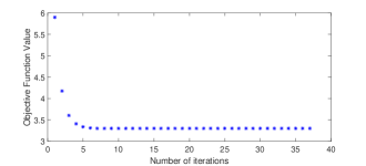
(a) Three sensors in three dimension

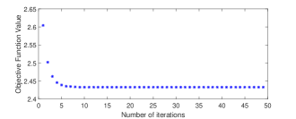
(b) Four sensors in three dimension

Figure 6: Value of the objective function of problem (11) plotted against the number of iterations for sensors with equal accuracies.

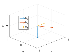
(a) Three sensors

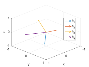
(b) Four sensors

Figure 7: Optimal configurations obtained by the proposed algorithm for simulation setup discussed in section IV-A.

IV-B Sensors with Different Accuracies and Uncorrelated Noise

In this section, we show some results for the case when the sensors have different accuracies and uncorrelated noise, that is, the measurement noise covariance matrix is diagonal with positive diagonal elements. The proposed algorithm converges to values mentioned in the table II and hence converges to the optimal solutions.

Table II: The objective function values at which the proposed algorithm converges for diagonal covariance matrices.

IV-C Sensors with correlated noise

In this section, we show the simulation result for the case when sensors have correlated noise, that is, the off-diagonal elements of the measurement noise covariance matrix, $\mathbf{R}$, are non-zero. We randomly choose $\mathbf{R}$ in $\mathbb{S}_{++}^{m}$, where $\mathbb{S}_{++}^{m}$ represents the set of positive definite matrices of dimension $m\times m$.

We take $m=5$, $n=3$, and choose $\mathbf{R}$ in $\mathbb{S}_{++}^{m}$. In figure 8a, the values of the objective function of problem (11) are plotted at each iteration. The value of the objective function decreases at each iteration and converges to a finite value and a optimal solution is achieved. The optimal configuration obtained by the proposed algorithm is shown in figure 8b.

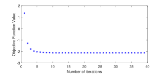
(a) The objective function of problem (11) plotted against the number of iterations.

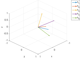
(b) Optimal configurations obtained by the proposed algorithm.

Figure 8: Simulation results for sensors with correlated noises.

V Conclusion

In this paper, a novel optimization algorithm which computes the optimal configuration for inertial sensors has been proposed. The proposed algorithm is based on the MM algorithm and the duality principle from the optimization theory. The proposed algorithm not only computes the optimal configuration for sensors with same accuracies but also for sensors with different accuracies and even for sensors having the correlated measurement noise.

In literature, optimal configurations are discussed and computed for sensors having same accuracies and measurement noises in sensors are uncorrelated. Here, we have extended the idea of optimal configuration for sensors having different accuracies and correlated noise.

The effectiveness of the proposed algorithm is verified via simulation results. The results show that the algorithm converges to the optimal solutions.

References

- [1] P. D. Groves, Principles of GNSS, inertial, and multisensor integrated navigation systems. Artech house, 2013.
- [2] J. W. Song and C. G. Park, “Optimal configuration of redundant inertial sensors considering lever arm effect,” IEEE Sensors Journal, vol. 16, no. 9, pp. 3171–3180, 2016.
- [3] A. Pejsa, “Optimum orientation and accuracy of redundant sensor arrays,” in 9th Aerospace Sciences Meeting, p. 59, 1971.
- [4] J. V. Harrison and E. G. Gai, “Evaluating sensor orientations for navigation performance and failure detection,” IEEE Transactions on Aerospace and Electronic Systems, no. 6, pp. 631–643, 1977.
- [5] L. Fu, X. Yang, and L. Wang, “A novel optimal redundant inertial sensor configuration in strapdown inertial navigation system,” in Position Location and Navigation Symposium (PLANS), 2012 IEEE/ION, pp. 240–246, IEEE, 2012.
- [6] M. Sturza, “Skewed axis inertial sensor geometry for optimal performance,” in Digital Avionics Systems Conference, p. 3874, 1988.
- [7] M. Jafari, “Optimal redundant sensor configuration for accuracy increasing in space inertial navigation system,” Aerospace Science and Technology, vol. 47, pp. 467–472, 2015.
- [8] M. Jafari and J. Roshanian, “Inertial navigation accuracy increasing using redundant sensors,” Journal of Science and Engineering, vol. 1, no. 1, pp. 55–66, 2013.
- [9] S. Sukkarieh, P. Gibbens, B. Grocholsky, K. Willis, and H. F. Durrant-Whyte, “A low-cost, redundant inertial measurement unit for unmanned air vehicles,” The International Journal of Robotics Research, vol. 19, no. 11, pp. 1089–1103, 2000.
- [10] R. Giroux, “Orthogonal vs skewed inertial sensors redundancy: A new paradigm for low-cost systems,” IFAC Proceedings Volumes, vol. 37, no. 5, pp. 97–102, 2004.
- [11] S. Guerrier, “Improving accuracy with multiple sensors: Study of redundant mems-imu/gps configurations,” in Proceedings of the 22nd international technical meeting of the Satellite Division of the Institute of Navigation (ION GNSS 2009), pp. 3114–3121, 2009.
- [12] D.-S. Shim and C.-K. Yang, “Optimal configuration of redundant inertial sensors for navigation and FDI performance,” Sensors, vol. 10, no. 7, pp. 6497–6512, 2010.
- [13] X. He, “Laplacian regularized D-optimal design for active learning and its application to image retrieval,” IEEE Transactions on Image Processing, vol. 19, no. 1, pp. 254–263, 2010.
- [14] S. Boyd and L. Vandenberghe, Convex optimization. Cambridge university press, 2004.
- [15] Y. Sun, P. Babu, and D. P. Palomar, “Majorization-minimization algorithms in signal processing, communications, and machine learning,” IEEE Transactions on Signal Processing, vol. 65, no. 3, pp. 794–816, 2017.
- [16] D. R. Hunter and K. Lange, “A tutorial on MM algorithms,” The American Statistician, vol. 58, no. 1, pp. 30–37, 2004.
- [17] T. Lipp and S. Boyd, “Variations and extension of the convex–concave procedure,” Optimization and Engineering, vol. 17, no. 2, pp. 263–287, 2016.
- [18] M. C. Grant and S. P. Boyd, “The cvx users’ guide, release 2.1,” CVX Research Inc, 2015.
- [19] M. Razaviyayn, M. Hong, and Z.-Q. Luo, “A unified convergence analysis of block successive minimization methods for nonsmooth optimization,” SIAM Journal on Optimization, vol. 23, no. 2, pp. 1126–1153, 2013.
- [20] S. Guerrier, “Integration of skew-redundant MEMS-IMU with GPS for improved navigation performance,” Master’s thesis, EPFL, Lausanne, Switzerland, 2008.