A survey of molecular cores in M17 SWex

Abstract

A survey of molecular cores covering the infrared dark cloud known as the M17 southwest extension (M17 SWex) has been carried out with the 45 m Nobeyama Radio Telescope. Based on the N₂H⁺ ($J=1-0$) data obtained, we have identified 46 individual cores whose masses are in the range 43 to 3026 ${M}_{\odot}$. We examined the relationship between the physical parameters of the cores and those of young stellar objects (YSOs) associated with the cores found in the literature. The comparison of the virial mass and the core mass indicates that most of the cores can be gravitationally stable if we assume a large external pressure. Among the 46 cores, we found four massive cores with YSOs. They have large mass of $\gtsim 1000M_{\odot}$ and line width of $\gtsim 2.5$ km s^-1 which are similar to those of clumps forming high mass stars. However, previous studies have shown that there is no active massive star formation in this region. Recent measurements of near-infrared polarization infer that the magnetic field around M17 SWex is likely to be strong enough to support the cores against self-gravity. We therefore suggest that the magnetic field may prevent the cores from collapsing, causing the low-level of massive star formation in M17 SWex.

1 Introduction

The infrared dark cloud M17 southwest extension (M17 SWex, Povich & Whitney, 2010), which is shaped like a “flying dragon” is located to the southwest of the M17 H ii region. A huge ($\sim 10^{6}M_{\odot}$) molecular cloud was found by the CO observations in the region using the Texas 5 m telescope with a beam size of $\sim 3\arcmin$ (Elmegreen & Lada, 1976). More recently, Busquet et al. (2013) conducted NH₃ observations using the Very Large Array and Effelsberg 100 m telescope toward a part of the high density region in M17 SWex, and they revealed a network of filaments constituting two hub-filament systems. The two hubs are dubbed “hub-N” and “hub-S”. Busquet et al. (2013) suggested that they are the main sites of stellar activity within the cloud.

Povich et al. (2016) suggested that M17 SWex has been an active star-forming region for the past $\gtsim 1$ Myr. Povich & Whitney (2010) identified 488 Young Stellar Objects (YSOs) in M17 SWex, and about 200 of the YSOs are found to be stars with a mass greater than $3M_{\odot}$ that will grow into B-type stars in the future. They suggested that M17 SWex probably has not yet formed its most massive star, predicted to be an early O-type star. From the 3 mm continuum emission observations toward the two hubs with ALMA, Ohashi et al. (2016) identified 48 cores and indicated that the internal turbulence is insufficient to prevent the gravitational collapse of the two hubs. They also suggested that clumps hosting the cores may be able to supply material to the cores. Povich et al. (2016) and Ohashi et al. (2016) speculate that mass accretion onto the cores via the hubs could produce massive star formation in the future. M17 SWex is thus considered to be in the early stages of formation of a new OB association (e.g., Elmegreen & Lada, 1976; Povich & Whitney, 2010). Therefore, M17 SWex is a molecular cloud suitable for study to explore the initial state of massive star formation. However, high-resolution observations of molecular emission lines in this region have been done only toward a limited area including hub-N and hub-S. The Millimeter Astronomy Legacy Team 90 GHz (MALT90) survey (Foster et al., 2011) revealed some dense cores in M17. A comprehensive molecular core survey in the cloud to cover the entire M17 SWex region is needed.

In other star forming regions, Shimoikura et al. (2018) found massive ($\sim 10^{3}M_{\odot}$) and dense ($\sim 10^{5}$ cm^-3 ) clumps with no massive stars. They suggested that such clumps are gravitationally stable without collapsing due to clump-supporting forces such as turbulence and magnetic fields. Sugitani et al. (2019) conducted near-infrared polarization observations toward M17 SWex. They revealed filament-like structures in the H₂ column density map, and found that the local magnetic field is perpendicular to most of the individual filamentary structures in high column density regions. They suggested that the magnetic field is likely to influence the formation and evolution of M17 SWex. To understand the relationship between the cores and the magnetic field in M17 SWex, it is necessary to identify dense cores in the region and to investigate the dynamical stability of the cores.

To search for dense cores in M17 SWex and to study their dynamics, we observed the region using the 45 m radio telescope at Nobeyama Radio Observatory (NRO) in some molecular lines at 93-115 GHz. In this study, we aim to identify the molecular cores in M17 SWex and catalog them using the N₂H⁺ molecular emission line at 93 GHz, which is a good tracer of dense gas. We investigate physical parameters of the cores and examine the relationship between physical properties of the cores and those of YSOs associated with the cores.

Povich & Whitney (2010) assumed that M17 SWex is at a distance of 2.0 kpc measured in the M17 H ii region based on the parallax measurements by Xu et al. (2011), since the LSR velocity $V_{\rm{LSR}}$ of M17 SWex and the H ii region are the same ($V_{\rm{LSR}}\simeq 20$ km s^-1). In our study, we also found that M17 SWex is likely to be connected to the H ii region, and thus we adopt 2.0 kpc as the distance to M17 SWex in this paper.

This study is based on “the Star Formation Legacy project” which is a large-scale survey of molecular gas in star forming regions. The outline of the project is presented by Nakamura et al. (2019a). Results of other regions are given in separate articles (OrionA: Nakamura et al. 2019b, Ishii et al. 2019, Tanabe et al. 2019, Aquila Rift: Shimoikura et al. 2019, Kusune et al. 2019, M17: Sugitani et al. 2019, NCS: Dobashi et al. 2019a, DR21: Dobashi et al. 2019b).

2 Observations

2.1 Observations with the NRO 45 m telescope

Observations of the ¹²CO, ¹³CO, C¹⁸O, CCS, and N₂H⁺ emission lines were carried out with the 45 m telescope at NRO. We observed the ¹²CO and ¹³CO emission lines for 20 hours in the period between 2015 April and 2016 March, and the other emission lines for 50 hours in the period between 2016 April and 2017 March. We used an on-the-fly (OTF) observing technique that was implemented for the 45 m telescope by Sawada et al. (2008). We observed whole of the M17 H ii region and M17 SWex ($\sim 1.5^{\circ}\times 0.5^{\circ}$) in the ¹²CO and ¹³CO lines. We also mapped an $\sim 1^{\circ}\times 0.5^{\circ}$ area in M17 SWex in the other lines. The beam size of the 45 m telescope is $\sim 15\arcsec$ (HPBW) at 100 GHz. We used the multi-beam receiver “FOREST” (FOur beam REceiver System on the 45 m Telescope; Minamidani et al., 2016) as the frontend and the digital spectrometer SAM45 as the backend. The velocity resolution was set to $0.04$ km s^-1 for the observed emission lines. The receiver provided a typical system temperature of 170 K. The pointing was checked every two hours by observing the SiO maser source V1111-Oph and was accurate within $5\arcsec$. The intensity calibration was made by observing a small region of $\sim 1\arcmin\times 1\arcmin$ in hub-N every time we tuned the receiver, and we found that the intensity fluctuations for all of the lines are less than $10\%$.

The data reduction for baseline subtraction was carried out using the NOSTAR software package developed at NRO. The 3D fits data were generated by convolving the observed data with a spheroidal function and regridding them at $7\farcs 5$ per pixel, resulting in an effective angular resolution of $22\arcsec-24\arcsec$, corresponding to a linear resolution 0.2 pc at a distance of 2.0 kpc. To increase the signal-to-noise ratios, we regridded the data to a velocity resolution of 0.1 km s^-1. We converted the antenna temperature $T_{\rm a}^{*}$ to the main beam temperature $T_{\rm{mb}}$ assuming that the main beam efficiency of the telescope is 0.416, 0.435, 0.437, 0.497, and 0.500 for the ¹²CO, ¹³CO, C¹⁸O, CCS, and N₂H⁺ emission lines, respectively. The rms noise of the final data is $\Delta T_{\rm{mb}}=0.4-1.0$ K. We summarize the observed molecular lines and the resulting noise levels in table 1. More detailed description for the data reduction are summarized by Nakamura et al. (2019a) and Shimoikura et al. (2019).

2.2 Archival data

We used the Herschel archival data of 160, 250, 350, and 500 $\micron$ toward M17 SWex to construct an H₂ column density $N$(H₂) map and a dust temperature $T_{\rm{dust}}$ map which are derived by fitting the spectral energy distribution (SED) of the Herschel data. Details of the data analysis are described by Sugitani et al. (2019). We regridded the maps of $N$(H₂) and $T_{\rm{dust}}$ onto the same grid as that of the molecular data obtained by the 45 m telescope.

3 Results

3.1 Spatial distributions of M17 SWex

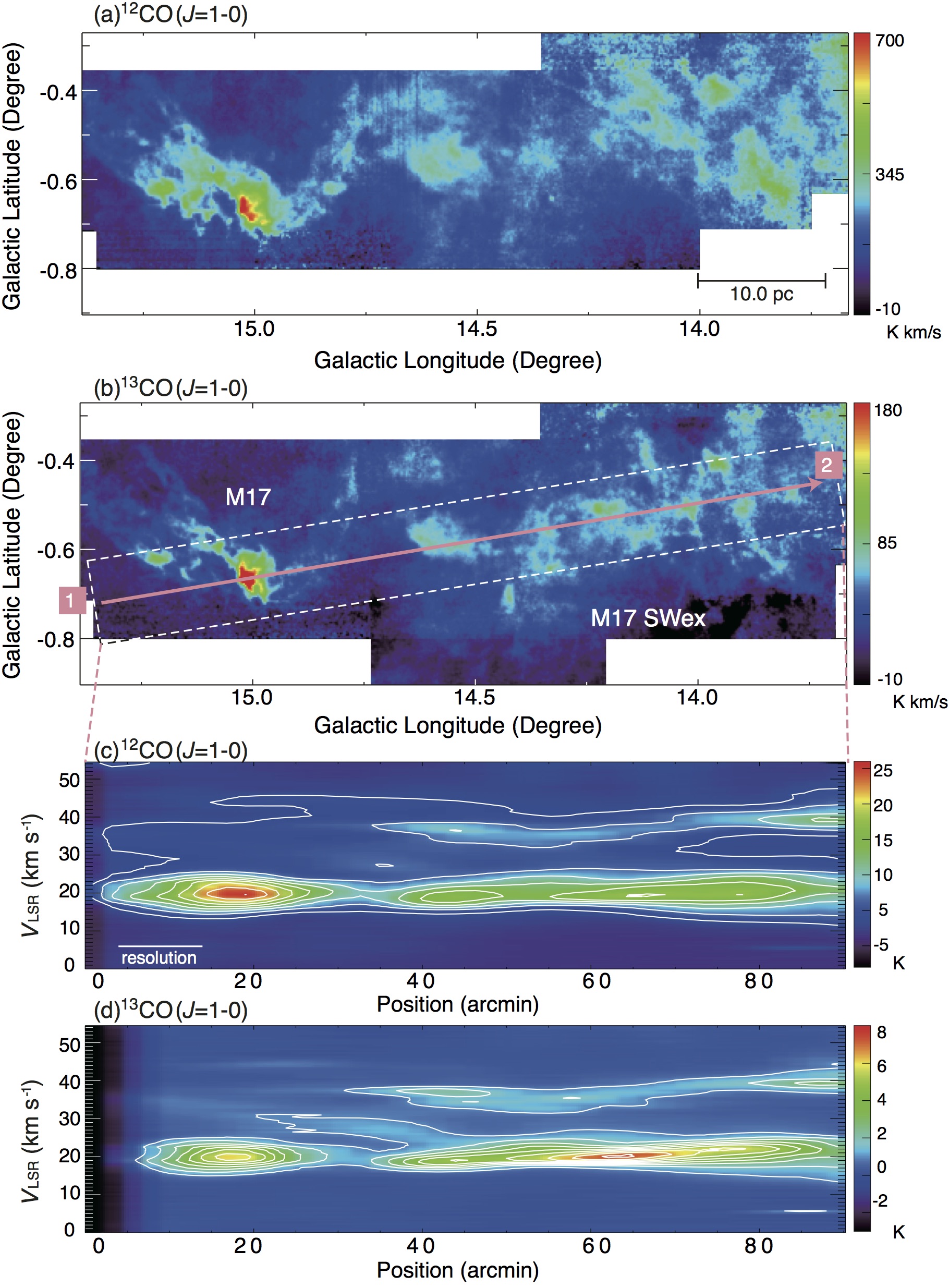
Figure 1: Integrated intensity maps of the (a) ¹²CO and (b) ¹³CO emission lines. The velocity ranges used for the integration is $-10.0\lesssim V_{\rm LSR}\lesssim 55.0$ km s^-1 for both of the emission lines. Position-velocity diagrams of the (c) ¹²CO and (d) ¹³CO emission lines taken along the cut (1)-(2) in panel (b). The lowest contour and the contour interval are both 3.0 K for panel (c) and are both 1.0 K for panel (d). As indicated in panel (b) by the white broken line, the angular resolution of the position-velocity diagrams is set to $10\arcmin$ to cover most of the cores identified in this study. The velocity resolution is set to 0.5 km s^-1.

Figure 1 shows the integrated intensity maps of the ¹²CO and ¹³CO emission lines. As we show in panels (c) and (d) of the figure, we made position-velocity (PV) diagrams across the M17 H ii region and M17 SWex along the line in panel (b). As seen in the figure, the intense emission lines around $V_{\rm{LSR}}=20$ km s^-1 smoothly change from the M17 H ii region to M17 SWex in terms of the radial velocity, line width, and the brightness temperature. We therefore assume that M17 SWex is physically connected with the M17 H ii region.

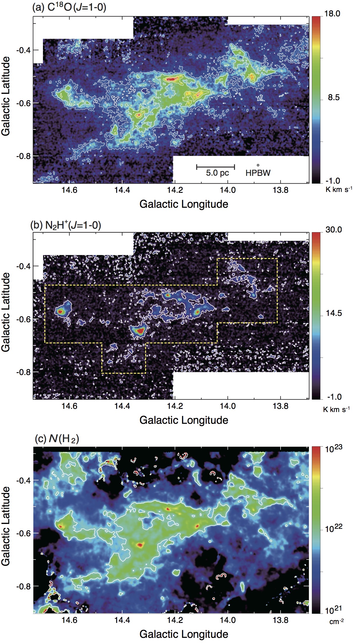
Figure 2: Integrated intensity maps of the (a) C¹⁸O and (b) N₂H⁺ emission lines. The velocity ranges used for the integration are (a) $15.0\lesssim V_{\rm LSR}\lesssim 26.0$ km s^-1 and (b) $6.0\lesssim V_{\rm LSR}\lesssim 34.0$ km s^-1. (c) The H₂ column density map derived from the Herschel data. The lowest contour and the contour interval for the C¹⁸O map are 4.0 K km s^-1. Contours are drawn at 2.8 K km^-1 and $1.0\times 10^{22}$ cm^-2 in the N₂H⁺ and $N$(H₂) maps, respectively.

Figure 2 shows the integrated intensity maps of the C¹⁸O and N₂H⁺ emission lines. CCS emission was not detected at the present sensitivity. The N₂H⁺ and C¹⁸O emission lines are distributed in the velocity range $6.0\lesssim V_{\rm{LSR}}\lesssim 34.0$ km s^-1 and $15.0\lesssim V_{\rm{LSR}}\lesssim 26.0$ km s^-1, respectively. The map of C¹⁸O traces well the shape of the flying dragon of the infrared dark cloud. Since the signal-to-noise ratio of the N₂H⁺ map is poor on the edge, we analyzed the data within the area surrounded by the yellow broken line shown on the map for N₂H⁺ in this study. For comparison, we also show the $N$(H₂) map calculated using the Herschel data by Sugitani et al. (2019) in figure 2(c). As seen in the panels (a) and (c), the distributions of C¹⁸O and $N$(H₂) show a good correlation. We also found that N₂H⁺ is distributed in regions where the $N$(H₂) density is relatively high ($\gtsim 10^{22}$cm^-2).

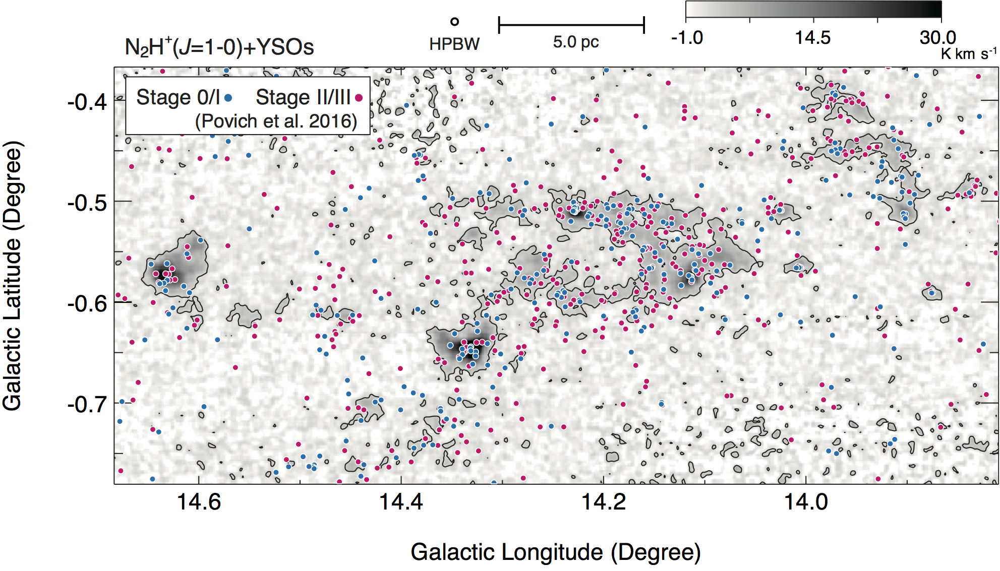
Figure 3: Distribution of YSOs associated with the M17 SWex region reported by Povich et al. (2016). The contours denote the N₂H⁺ integrated intensity map same as in figure 2 (b). Stage 0/I is the YSO accompanied by an infalling envelope, Stage II is the YSO with an optically thick circumstellar disk, Stage III is the YSO with an optically thin disk (see Povich & Whitney, 2010).

Povich & Whitney (2010) made a YSOs survey around M17 SWex. In the catalog they compiled, a total of 488 YSOs classified as Stage 0/I (YSOs accompanied by an infalling envelope), Stage II (YSOs with optically thick circumstellar disk), Stage III (YSOs with optically thin disk), and “Ambiguous stage” are listed. Povich et al. (2016) updated the catalog. In the catalog, 840 stars are classified as Stage 0/I, Stage II/III, and Ambiguous stage. We show the distributions of these YSOs associated with the observed region using the catalog of Povich et al. (2016) in figure 3. We found that the Stage 0/I YSOs are distributed in dense parts of the N₂H⁺ emission whereas the Stage II and III YSOs are distributed more randomly throughout the M17 SWex region.

3.2 Identification of cores

In order to identify cores based on the N₂H⁺ emission, we apply the “dendrogram” algorithm (e.g., Rosolowsky et al., 2008) to the N₂H⁺ integrated intensity map. The dendrogram identifies three hierarchical structures of “leaf”, “branch”, and “trunk”. We chose the minimum threshold intensity required to identify a parent tree structure to be $4\,\sigma$ (=2.8 K km s^-1) and a splitting threshold intensity required to identify structures to be $2\,\sigma$. We only consider leaves with at least 25 pixels which are the equivalent area of the synthesized beam ($0.39$ arcmin²), and we refer to them as “cores”. As a result, a total of 46 cores are identified. We note that the results of the above core identification, e.g., the number and position of the cores, do not change significantly with other algorithms such as “clumpfind”.

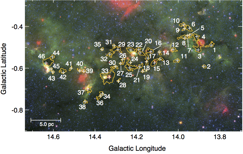
Figure 4: Distribution of the identified cores. The background is a $\it{Spitzer}$ composite image made with the $24.0\micron$ (red), $8.0\micron$ (green) and $3.6\micron$ (blue) data. The identified cores are numbered in the order of galactic longitude. The white plus sign is the peak position of the N₂H⁺ integrated intensity of each core. Orange contours denote the surface area of the cores defined at $2.8$ K kms ^-1 ($=4\sigma$).

Figure 4 shows the cores identified. We numbered the identified cores from No.1 to No.46 in the order of galactic longitude. We searched for YSOs in the catalog of Povich et al. (2016) within the boundary of the cores and found that there are 40 cores with YSOs and 6 cores without YSOs. We assume that the YSOs are associated with the cores. The peak position of the cores and the number of YSOs associated with each core are summarized in table 2. We found that four cores (Nos. 15, 23, 33, and 46) are especially large having a size of $\sim 1$ pc. These cores are accompanied by many YSOs. Among these, two cores correspond to the regions known as hub-N (=No. 33) and hub-S (=No. 15).

The distances to some of the detected cores can be found in the literature, but there is an uncomfortable mismatch. Wu et al. (2014) determined the distance of G$14.63-0.57$ (= core No.46) to be $1.83^{+0.08}_{-0.07}$ kpc by a parallax measurement. On the other hand, Sato et al. (2010) reported a distance of $1.12\pm 0.13$ kpc for G$14.33-0.64$(= core No. 33) which is located not far from G14.63-0.57 on the plane of the sky. Povich et al. (2016) suggested that G$14.63-0.57$ is actually much closer than the other core. However, as can be seen in figure 1, the radial velocities, line widths, and intensities of the observed ¹²CO and ¹³CO lines change smoothly over the entire M17 SWex region including cores No. 33 and 46, suggesting that they may belong to the same system. In this paper, we assume that all of the cores identified in this work are located at 2.0 kpc (Xu et al., 2011) for simplicity. Parameters of the cores derived in this paper should be rescaled when their distances are established precisely. Complexity of the distance measurements of the M17 SWex region in the literature is summarized and discussed by Povich et al. (2016) in detail.

3.3 Physical parameters derived from the molecular line data

Assuming local thermodynamic equilibrium (LTE), we estimated the physical parameters of the cores.

In order to derive the excitation temperature based on the ¹²CO data as well as to derive the column density of C¹⁸O, we followed the method described by Shimoikura et al. (2018). Using the optically thick ¹²CO line ($\tau\gg 1$), we estimated the excitation temperature $T^{\rm{co}}_{\rm ex}$ at the individual positions in the observed region. The ¹²CO emission is widely distributed over the whole region in the observed velocity range (see figure 1). The peak intensity of the ¹²CO spectra was measured for M17 SWex in the velocity range from 0 to 30 km s^-1, and we determined $T^{\rm{co}}_{\rm ex}$ by measuring the peak brightness temperature of the ¹²CO line in this velocity range. Finally, the C¹⁸O column density $N$(C¹⁸O) was calculated from the C¹⁸O intensity.

Next, we derived the physical parameters of the N₂H⁺ molecular emission line. The procedure for the derivation is similar to that described by Shimoikura et al. (2019). We fitted the seven hyperfine components with multiple Gaussian functions under the assumption that all of the seven hyperfine lines have a single line width and excitation temperature. The fitting was performed to the spectra within the area where the cores were identified. We then derived the peak temperature $T_{\rm{mb}}$, the centroid velocity $V_{\rm{LSR}}$, the line width $\Delta V$, the excitation temperature $T^{\rm{N{{}_{2}}H^{+}}}_{\rm ex}$, and the total optical depth $\tau_{\rm{tot}}$ for all of the hyperfine components. When the emission line is optically thin, $\tau_{\rm{tot}}$ and $T^{\rm{N{{}_{2}}H^{+}}}_{\rm ex}$ cannot be estimated well simultaneously by the fitting. For such spectra, we estimated $T^{\rm{N{{}_{2}}H^{+}}}_{\rm ex}$ by interpolating $T^{\rm{N{{}_{2}}H^{+}}}_{\rm ex}$ at the neighboring positions with a weighted two-dimensional Gaussian function. We then estimated the N₂H⁺ column density $N$(N₂H⁺) using the line parameters derived above (see Shimoikura et al., 2019).

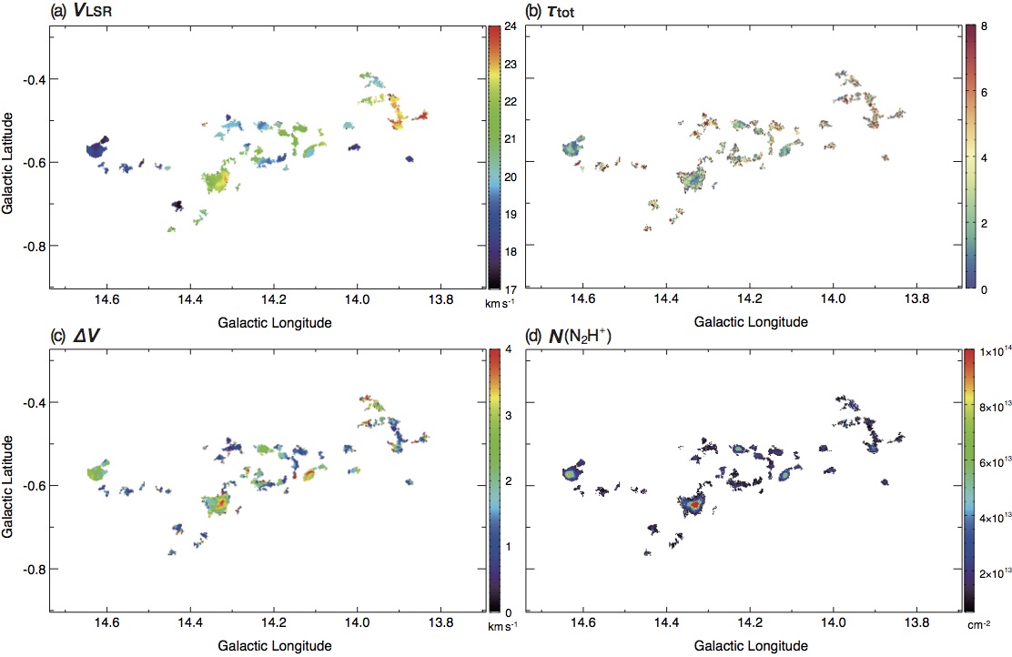
Figure 5: (a) The centroid velocity map, (b) total optical depth map, (c) line width map, and (d) column density map of the N₂H⁺ emission line. These maps are obtained based on the hyperfine spectra fitting of the N₂H⁺ data.

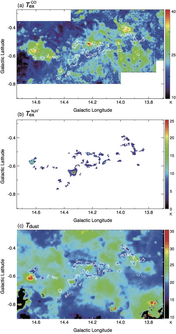
Figure 6: (a) Excitation temperature map derived from the ¹²CO data. (b) Excitation temperature map derived from the N₂H⁺ data. (c) Dust temperature map derived from the Herschel data. The cores shown in figure 4 are overlaid in panels (a) and (c) by the white contours.

In figure 5, we present each parameter map obtained from the hyperfine spectra fitting. The line parameters of the peak positions of the cores are summarized in table 3. The distributions of the temperatures $T^{\rm{co}}_{\rm ex}$, $T^{\rm{N{{}_{2}}H^{+}}}_{\rm ex}$, and $T_{\rm{dust}}$ are shown in figure 6.

For each core, we measured the surface area $S$ at the 2.8 K km s^-1 (=$4\,\sigma$) contour level shown in figure 4, and the radius $R_{\rm core}$ defined as $R_{\rm core}=\sqrt{S/\pi}$. Next, using the $N(\rm{H}_{2})$ data obtained from the optically thin dust data by Hershel, we estimated the mass of the core $M_{\rm{core}}$ as

$$M_{\rm{core}}=\mu m_{\rm{H}}S\times\Sigma N(\rm{H}_{2}),$$ (1)

where $\mu$ is the mean molecular weight (2.8) and $m_{\rm{H}}$ is the hydrogen mass.

We assume that the cores are a sphere of radius $R_{\rm core}$ with uniform density and temperature. When the cores are dynamically stable, the virial theorem (Spitzer, 1978) can be written as

$$4\pi{R_{\rm core}}^{3}P_{\rm ext}=\frac{3kT}{\mu m_{\rm H}}{M_{\rm core}}-\frac{3G}{5R_{\rm core}}{M^{2}_{\rm core}}\ ,$$ (2)

where $P_{\rm ext}$ is the external pressure by the surrounding gas, $k$ is the Boltzmann constant, and $G$ is the gravitational constant. We assume temperature of the cores $T$ can be expressed as $T={\mu m_{\rm H}}\Delta V^{2}/8k(\rm{ln}2)$ which is equivalent to the Doppler temperature of the gas. We then estimated the virial mass $M_{\rm vir}$ at $P_{\rm ext}$=0 using

$$M_{\rm vir}=\frac{5R}{G}\frac{{\Delta V}^{2}}{8\,{\rm ln}2}\ ,$$ (3)

where ${\Delta V}$ is the line width obtained by the hyperfine fitting at the peak position of the cores. We list the derived parameters in table 4.

Furthermore, the fractional abundances of C¹⁸O and N₂H⁺, $f$(C¹⁸O) and $f$(N₂H⁺), respectively, are directly derived from the ratios of each column density and $N$(H₂).

The constants of the observed molecular lines used to derive the parameters in this section are summarized by Shimoikura et al. (2018, see their table 2). We found that the derived parameters are in the ranges $0.2\lesssim R_{\rm core}\lesssim 1.0$ pc, $43\lesssim M_{\rm core}\lesssim 3026$ ${M}_{\odot}$, $3.00\lesssim T^{\rm{N{{}_{2}}H^{+}}}_{\rm ex}\lesssim 31.68$ K, and $0.76\lesssim\Delta V\lesssim 4.00$ km s^-1. Among the 46 cores, we found the four massive cores (Nos. 15, 23, 33, and 46) with a mass of more than $1000M_{\odot}$. These cores have larger $\Delta V$ ($\gtsim 2.5$ km s^-1) and higher $T^{\rm{N{{}_{2}}H^{+}}}_{\rm ex}$ ($\gtsim 10$ K) than the other cores. $T^{\rm{N{{}_{2}}H^{+}}}_{\rm ex}$and $\Delta V$ of the other cores are $<10$ K and $<2$ km s^-1, respectively, indicating that $T^{\rm{N{{}_{2}}H^{+}}}_{\rm ex}$ and $\Delta V$ increase as $M_{\rm core}$ increases.

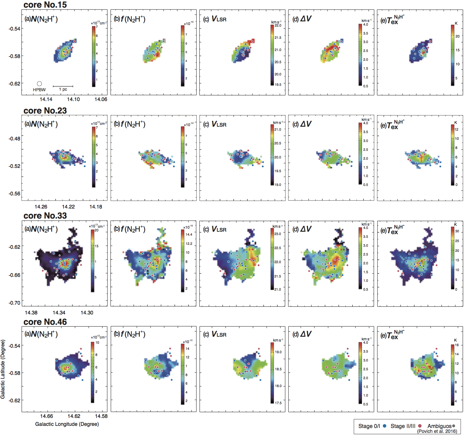
Figure 7: The N₂H⁺ parameter maps for cores No. 15, 23, 33, and 46. (a) The $N$(N₂H⁺) map. (b) The $f$(N₂H⁺) map. (c) The $V_{\rm LSR}$ map. (d) The $\Delta V$ map. (e) The $T^{\rm{N{{}_{2}}H^{+}}}_{\rm ex}$ map.

Busquet et al. (2013) revealed that the velocity dispersion is locally enhanced ($\sigma\sim 1$ km s^-1) toward hub-N (No.23) and hub-S (No.15). Based on the SMA images, Busquet et al. (2016) show that the two hubs fragment into several dust condensations. The large $\Delta V$ of the four cores suggest that there are multiple unresolved sub-cores not only in cores No. 15 and 23 but also in cores No. 33 and 46. In figure 7, we show the parameter maps for the four cores. It seems that there is a correlation between the distributions of $T^{\rm{N{{}_{2}}H^{+}}}_{\rm ex}$ and those of YSOs. In addition, it appears that there is an anti-correlation between the distributions of $f$(N₂H⁺) and those of YSOs. For the relationships between the distribution of $\Delta V$ and those of YSOs, the correlation is not clear.

3.4 Correlation between $N$(N₂H⁺) and $N$(H₂) for the cores

To estimate the total masses of cores from $N$(N₂H⁺), abundance ratio of $f$(N₂H⁺)$=3\times 10^{-10}$ reported by Caselli et al. (1995) has widely been used in star-forming regions. However, as seen in figure 7, $f$(N₂H⁺) varies even within a single core. In this study, we investigate the relationship between $N$(N₂H⁺) and $N$(H₂) of the identified cores.

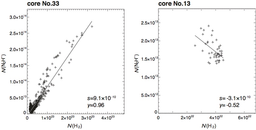
Figure 8: The relation between $N$(N₂H⁺) and $N$(H₂) for cores No.33 (left) and 13 (right).

For each of the cores, we made a plot of $N$(N₂H⁺) vs. $N$(H₂), and found that $N$(N₂H⁺) correlates roughly linearly with $N$(H₂) in most cases. We show two examples in figure 8. We performed a linear least-square fit to the plots as,

$$N(\rm{N}_{2}H^{+})=\it{sN}({\rm{H}_{2}})+\it{i}$$ (4)

where $s$ and $i$ are the slope and intercept of the linear relation, respectively. In general, $N$(N₂H⁺) represents the column density only of the limited region denser than the critical density to excite the N₂H⁺ line, but $N$(H₂) derived from the dust emission traces the total column density along the line-of-sight including the diffuse surroundings. Therefore, $i$ in the above can be used to remove the contribution from the low density regions not emitting the N₂H⁺ line, and $s$ should better trace the average fractional abundance of N₂H⁺ in the cores.

In table 5, we summarize the obtained values of $s$ and $i$ together with the correlation coefficients $\gamma$. As listed in the table, there is a large variation in $s$, and its median value is $s=3.5\times 10^{-10}$ which is consistent with those measured in other clouds (e.g., Tanaka et al., 2013; Shimoikura et al., 2019).

Among the detected 46 cores, there are 15 cores showing a good correlation with $\gamma\gtsim 0.6$, and 14 cores showing almost no correlation ($\gamma\ltsim 0.2$). Most of the cores have a positive value of $s$($>0$), but there are some cores having negative values ($s<0$, e.g., core No. 13), suggesting that N₂H⁺ is probably adsorbed onto dust in the densest part of the cores (e.g., Bergin et al., 2002; Belloche & André, 2004).

3.5 Relationship between the cores and YSOs

We attempt to investigate the relationship between the mass of the cores and those of YSOs forming in the cores. For this, we estimated the total stellar mass $\Sigma M_{\star}$ associated with each core. The catalogue of Povich & Whitney (2010) contains a number of good candidate YSOs, but some of the estimated parameters such as the stellar mass could be erroneous due to ambiguities of the adopted model. We therefore made use of the newer catalog by Povich et al. (2016) which is more complete but does not present stellar masses, and we adopted the following rough method to estimate $\Sigma M_{\star}$: First, we counted the catalogued YSOs located within the extent of each core, and assumed that the median value of their masses is $M_{\rm medi}=3$ ${M}_{\odot}$ (Povich 2019, private communication). Second, we assumed the stellar initial mass function (IMF) by Kroupa (2001) and scaled the IMF to match the observed number of YSOs having a mass greater than $M_{\rm medi}$ in each core. Finally, we estimated $\Sigma M_{\star}$ in the cores by integrating the scaled IMF. Resulting values of $\Sigma M_{\star}$ are summarized in the last column of table 4. The total stellar mass in the table amounts to $\sim 2900$ ${M}_{\odot}$.

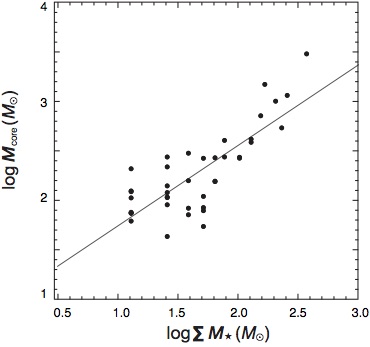
Figure 9: The core mass $M_{\rm{core}}$ vs. the total stellar mass $\Sigma M_{\star}$. The solid line is the least-squares fit given in eqation 5.

In figure 9, we display the relation of $M_{\rm{core}}$ vs. $\Sigma M_{\star}$ in logarithmic scale. They are roughly correlated, and the relation can be fitted as

$${\rm log}\ M_{\rm core}=(0.93\pm 0.17)+(0.81\pm 0.10){\rm log}\ \Sigma M_{\star}\$$ (5)

where $M_{\rm core}$ and $\Sigma M_{\star}$ are in units of $M_{\odot}$. The index ($0.81$) is close to unity, indicating that the total stellar mass is roughly proportional to the natal core mass.

3.6 Star Formation Efficiency of M17 SWex

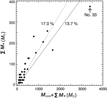
Figure 10: The total stellar mass of YSOs associated with each core $\Sigma M_{\star}$ vs. the total mass of the system for each core ($M_{\rm core}+\Sigma M_{\star}$). The linear least-square fit (SFE=$13.7\%$) is shown by the solid line. The broken line denotes the best fit when we exclude the core No.33 from the fit.

We show a plot of $\Sigma M_{\star}$ vs. $M_{\rm core}$+$\Sigma M_{\star}$ in figure 10. Star Formation Efficiency (SFE) is a fundamental parameter of cluster-formation process (Lada & Lada, 2003) and is calculated as $\Sigma M_{\star}/(M_{\rm core}+\Sigma M_{\star}$ ). We investigated the SFE of M17 SWex by fitting the all of the data points in figure 10. The result is shown in the figure by the solid line which corresponds to SFE$=13.7\%$. Many of the data points smaller than $M_{\rm core}+\Sigma M_{\star}=2000$ $M_{\odot}$ are above the solid line because of core No. 33, whose distance might be very different from the other cores (see section 3.2). We would obtained SFE$=17.0\%$ if we exclude this core from the fit (the broken line in the figure). The total SFE obtained from the total stellar mass ($\sim 2920$ $M_{\odot}$) and the total mass of the cores ($\sim 14300$ $M_{\odot}$) is $16.9\%$.

As seen in figure 3, there are YSOs outside the extents of the detected cores. Povich & Whitney (2010) estimated $\Sigma M_{\star}$ for M17 SWex to be $8\times 10^{3}M_{\odot}$ by integrating the IMF of Kroupa (2001) over $M_{\star}\gtsim 0.1M_{\odot}$. We estimated the total gas mass of the entire M17 SWex region to be $7.8\times 10^{4}M_{\odot}$ by integrating $N(\rm{H}_{2})$ within the area defined by the $1.0\times 10^{21}$ H₂ cm^-2 contour. These values infer a average SFE of $9.3\%$ for the entire M17 SWex region.

According to Lada & Lada (2003) who cataloged the SFEs for nearby embedded clusters, the SFEs range from approximately 10 to 30 $\%$. The values of $9.3\%$ and $\sim 17\%$ obtained in M17 SWex is comparable to those of the cluster-forming regions.

4 Discussion

4.1 Dynamical state of the cores

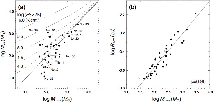
Figure 11: (a) Relationship between $M_{\rm vir}$ and $M_{\rm core}$. Filled and open circles represent the cores with and without YSOs, respectively. The solid line shows the external pressure $P_{\rm ext}$ = 0 where$M_{\rm core}=M_{\rm vir}$, and the dotted line show the virial masses in equilibrium with the external pressure log ($P_{\rm ext}/k$) = 4.0, 4.5, 5.0, 5.5, 6.0 K cm^-3. (b) Relationship between $R_{\rm core}$ and $M_{\rm core}$. The black line shows the fitting result of the relation ($R_{\rm core}=0.05M_{\rm core}^{0.37}$, see text).

We investigate the dynamical state of the cores. Figure 11(a) shows the relation between $M_{\rm{vir}}$ and $M_{\rm{core}}$. The solid line indicates $M_{\rm{core}}=M_{\rm{vir}}$. Focusing on the relationship between $M_{\rm{core}}$ and $M_{\rm{vir}}$, the observed cores can be divided into the following three types, and we discuss their characteristics.

1. We found that many cores satisfy the condition of $M_{\rm{core}}\simeq M_{\rm{vir}}$, indicating that the cores are dynamically stable if there is no external pressure ($P_{\rm ext}$=0). More massive cores tend to be in the gravitational virial equilibrium.

2. Cores satisfying the condition of $M_{\rm{core}}>M_{\rm{vir}}$ may be contracting because they cannot prevent collapsing by the internal pressure even when $P_{\rm ext}$=0. The value of $\Delta V$ for such cores (e.g., cores No.1 and 28) is relatively small, being less than 1 km s^-1 (table 3).

3. There are some cores under the condition of $M_{\rm{core}}<M_{\rm{vir}}$ (e.g., cores No.10 and 35), and such cores will disperse under the condition $P_{\rm ext}=0$. However, they can be confined in the pressure of the high density gas surrounding the cores. We suggest that such cores are highly influenced by $P_{\rm ext}$ in equation 2. Virial mass taking into account $P_{\rm ext}$ can be expressed as,

   $${M_{\rm vir}}={M_{\rm core}}+\frac{20\pi}{3G}{\rm{A}}{M^{4{\rm B}-1}_{\rm core}}P_{\rm ext}\ ,$$ (6)

   where A and B are constants to relate $M_{\rm core}$ and $R_{\rm{core}}$ as $R_{\rm{core}}={\rm A}M^{\rm B}_{\rm core}$. We derived A = 0.05 and B = 0.37 for $R_{\rm{core}}$ and $M_{\rm core}$ in units of pc and $M_{\odot}$, respectively, by fitting the plot shown in figure 11(b) with the relation. In figure 11(a), we show $M_{\rm{vir}}$ by the broken lines calculated based on equation 6 for various $P_{\rm ext}(\neq 0)$. As seen in the figure, comparing the position of the plot with the lines, most of the cores can be dynamically stable under $P_{\rm ext}/k=10^{5.0}-10^{5.5}$ K cm^-3.

In summary, we suggest that many of the cores can be dynamically stable if we assume a large external pressure. For cores under the condition $M_{\rm{core}}>M_{\rm{vir}}$, the internal pressure due to turbulence is too small, and they should contract by the self-gravity if there is no magnetic field strong enough to support them. We will further discuss this point in section 4.3.

4.2 Density structure of the cores

We investigate the distribution of $N({\rm{H}_{2}})$ of the cores as a function of the projected distance $R$ from the peak of $N({\rm{H}_{2}})$. We found that profile of $N({\rm{H}_{2}})$ for the cores are found to be different for each core. In the case of a spherical core, we assume that the number density of H₂ molecules $\rho$ is expressed as $\rho(r)\propto r^{-\alpha}$, where $r$ is the distance from the center of the sphere. The physical state of the cores can be estimated by examining the value of $\alpha$. For example, a density profile of gravitationally stable cores and free-falling cores show $\alpha=2.0$ and 1.5, respectively (e.g., Shu, 1977; Motte & André, 2001; Shimoikura et al., 2016).

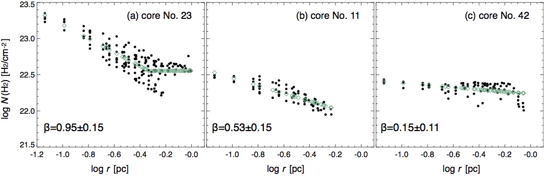
Figure 12: The distribution of $N({\rm{H}_{2}})$ as a function of the projected distance from the peak of $N({\rm{H}_{2}})$ for cores (a) No. 23, (b) No.11, and (c) No.42. Green diamond represents a fit (see text).

To investigate the density structure of the cores, we fitted the relations between $N({\rm{H}_{2}})$ and $R$ of the cores with $N({\rm{H}_{2}})=N_{0}(R/R_{0})^{-\beta}+C$ where $N_{0}$, $R_{0}$, and $C$ are constants. The obtained values of the index $\beta$ are roughly divided into three types: (a) $0.7-1.2$ for the four massive cores, (b) $0.3-0.6$ for the smaller cores with YSOs, and (c) $0.1-0.3$ for the cores without YSOs. Because $\beta=\alpha-1$, the values of $\beta$ infer $\alpha=1.7-2.2,1.3-1.6$, and $1.1-1.3$ for the cases (a), (b), and (c) in the above, respectively. In figure 12, we show typical examples of the $N$(H₂) vs. $R$ relations for the 3 types. There are 4, 28, and 14 cores belonging the types (a), (b), and (c), respectively.

The results suggest that the cores of (a) and (b) types are likely to be gravitationally stable and free-falling, respectively. Note that, in the case of the type (c) cores, they show a flat density profile and there is a possibility that the cores are not resolved at the present resolution due to their small size.

4.3 Star formation in M17 SWex

As found in section 4.1, some of the cores satisfy the condition $M_{\rm{core}}>M_{\rm{vir}}$, which means that the cores are contracting if we ignore the effects of the magnetic field. Ohashi et al. (2016) observed small cores in the two hubs identified with ALMA observations which correspond to the cores No.12–23 in our work. They found that the small cores have viral parameters (defined as $M_{\rm{vir}}/M_{\rm core}$) in the range 0.1-1.3, which is comparable to our results. Based on the analysis of the virial parameters, Ohashi et al. (2016) speculated that mass accretion onto the cores via the hubs could produce massive stars in the future. However, their values of the virial parameters do not take into account the effect of the magnetic field. In order to investigate whether the cores are really contracting or not, a quantitative estimate of the magnetic field is needed.

Recently, Sugitani et al. (2019) conducted near-infrared polarization observations toward M17 SWex, and revealed the overall distribution of the magnetic field around the individual filamentary structures. They found that the magnetic field in M17 SWex is mostly perpendicular to the elongation of the filamentary clouds, and they estimated the strength of the magnetic field to be $70-300$ $\mu$G using the Davis-Chandrasekhar-Fermi method. Based on these results, Sugitani et al. (2019) suggested that the clouds in M17 SWex are likely to be magnetically critical or sub-critical, which may be responsible for the present low-level of massive star formation in M17 SWex.

The critical mass of the cores that can be supported by the magnetic field is expressed as $M_{\rm{cr}}/M_{\odot}\simeq 2\times 10^{2}(B/30\mu$G)($R_{\rm core}/1$pc)² (e.g., Nakano & Yoshida, 1986; Shu et al., 1987). Using $R_{\rm core}$ and $M_{\rm core}$ in table 4, we found that the magnetic field of $\sim 100-600$ $\mu$G is necessary for these cores to be magnetically critical. The range of the magnetic field is consistent with or slightly larger than the values $70-300$ $\mu$G reported by Sugitani et al. (2019). We should note that Sugitani et al. (2019) measured the magnetic field at the periphery of M17 SWex where the background stars were well detected in the near-infrared, and thus, the magnetic field inside the dense cores can be stronger than the values they obtained, if the magnetic field is frozen into the dense cores. In addition, their values are for the component projected on the plane of the sky but do not include the component parallel to the line-of-sight. As Sugitani et al. (2019) suggested, we conclude that the cores detected in this study are likely to be magnetically critical or sub-critical, and the magnetic field prevents the cores from collapsing, which may be the cause of the inactive massive star formation in M17 SWex.

However, it is rather mysterious that the total SFE of M17 SWex ($\sim 9-17\%$) is comparable to those of other cluster-forming clumps producing massive stars (section 3.6), indicating that low-mass (and intermediate-mass) stars are forming in spite of the magnetic fileds. We imagine that small cores producing the small stars, which may not be detected by our observations, can lose the supporting force by the magnetic field soon via the ambipolar diffusion because of their small sizes. In addition, sporadic collisions of the internal substructures of the cores/clumps (such as “fibers”) may also induce formation of low-mass stars via sudden increment of density (Dobashi et al., 2014; Matsumoto et al., 2015). These effects can help the formation of low-mass stars. For the massive cores we identified in M17 SWex, we suggest that they are unlikely to collapse at the moment due to the support by the magnetic field, but they may eventually become supercritical to collapse and form massive stars if they lose the clump-supporting force by the magnetic field, or if they gain more mass via mass accretion from the surroundings.

5 CONCLUSIONS

An N₂H⁺ survey for molecular cores was made toward the M17 southwest extension (M17 SWex) region. We identified 46 molecular cores. Among the 46 cores, 40 of them are associated with Young Stellar Objects (YSOs) and the other 6 cores are not associated with any YSOs. Investigation of the core properties was also done by using the ¹²CO, ¹³CO, and C¹⁸O data as well as $N$(H₂) the column density of H₂ and the dust temperature derived from Herschel data. We also used physical properties of YSOs found in the literature.

We summarize the main findings of this study as follows:

1. We derived the masses of the individual cores from the $N$(H₂) data assuming a distance of 2.0 kpc, and found that the core masses vary in the range from 43$M_{\odot}$ to 3026$M_{\odot}$. Based on the N₂H⁺ data, we derived the physical parameters of the cores and presented each parameter map. The derived excitation temperature and the line width range from 3.0 K to 31.7 K and from 0.8 km s^-1 to 4.0 km s^-1, respectively. Among the 46 cores, we found four massive cores associated with YSOs. The cores have a large mass of $\gtsim 1000M_{\odot}$, a line width of $\gtsim 2.5$ km s^-1, and an excitation temperature of $\gtsim 10$ K.

2. We investigated the fractional abundance of N₂H⁺ for all of the cores. The values are estimated to be in the range $(4-10)\times 10^{-10}$, indicating that there is a large variation among the cores.

3. We estimated the average star formation efficiency of M17 SWex to be $\sim 9-17\%$.

4. Comparison of the virial mass and the core mass estimated from the Herschel data revealed that most of the cores can be dynamically stable if we assume a large external pressure. For some cores, the results of the comparison indicate that internal pressure due to turbulence is small, and they can collapse by the self-gravity if there is no internal supporting force by the magnetic field.

5. Assuming a radial density profile of spherical gas, we examined the $N$(H₂) distribution to infer the index $\alpha$ of the density profile of the cores $\rho(r)\propto r^{-\alpha}$. We found that 32 out of 46 cores have a value of $\alpha$ in the range $1.3-2.2$, suggesting that the cores are gravitationally stable or free-falling.

6. We estimated that the magnetic field of $\sim 100-600$ $\mu$G is required for the cores to be critical. This value is comparable to the strength of the magnetic filed recently measured by Sugitani et al. (2019). Previous studies (e.g., Povich & Whitney, 2010) have shown that there is no active massive star formation in M17 SWex, and we suggest that it is due to the cloud-supporting force by the magnetic field which prevents the cores from collapsing.

We thank Dr. M. S. Povich for his reviewing this paper and for a number of useful comments. We are also grateful to the other members of Star Formation Legacy project for their support during the observations. This work was supported by JSPS KAKENHI Grant Numbers JP17K00963, JP17H02863, JP17H01118, JP16K12749, and NAOJ ALMA Scientific Research Grant Numbers 2017-04A. YS also received support from the ANR (project NIKA2SKY, grant agreement ANR-15-CE31-0017). The 45 m radio telescope is operated by NRO, a branch of NAOJ.

Table 1: The observed molecular lines

Molecule	Transition	Frequency	Beam	$\Delta T_{\rm mb}$
		(GHz)		(K)
N2H+	$J=1-0$	93.1737637	$17\farcs 9$	0.44
CCS	$J_{N}$=8${}_{7}-7_{6}$	93.8700980	$17\farcs 8$	0.42
C18O	$J=1-0$	109.7821760	$15\farcs 2$	0.43
13CO	$J=1-0$	110.2013540	$15\farcs 1$	0.37
12CO	$J=1-0$	115.2712040	$14\farcs 5$	0.90

The rest frequency for the N₂H⁺ line is taken from Pagani et al. (2009), and those of the other lines are taken from the website of Lovas (1992).

Table 2: The cores and associated YSOs

			number of YSOs
Core	$l$	$b$	Stage 0/I	Stage II/III	A
	(∘)	(∘)
1	13.84	-0.49	1	7	0
2	13.88	-0.59	2	1	0
3	13.90	-0.51	10	2	0
4	13.91	-0.45	2	0	0
5	13.94	-0.44	0	2	0
6	13.95	-0.41	0	3	2
7	13.96	-0.44	0	2	2
8	13.97	-0.46	4	0	1
9	13.97	-0.41	0	0	1
10	13.97	-0.39	3	1	0
11	14.00	-0.56	3	2	0
12	14.02	-0.51	4	2	2
13	14.09	-0.56	1	0	0
14	14.09	-0.52	0	0	0
15	14.11	-0.57	9	3	4
16	14.13	-0.52	4	6	0
17	14.15	-0.55	1	1	2
18	14.15	-0.57	1	0	0
19	14.17	-0.61	3	0	1
20	14.18	-0.53	5	4	1
21	14.19	-0.59	0	2	1
22	14.19	-0.51	2	3	1
23	14.23	-0.51	11	8	1
24	14.23	-0.57	0	1	1
25	14.23	-0.60	8	6	4
26	14.27	-0.56	1	0	0
27	14.28	-0.58	3	1	0
28	14.29	-0.66	0	1	0
29	14.29	-0.51	2	1	3
30	14.30	-0.59	1	2	0
31	14.31	-0.49	1	0	0
32	14.33	-0.53	0	0	0
33	14.33	-0.65	14	11	4
34	14.36	-0.72	0	1	0
35	14.37	-0.51	0	0	0
36	14.37	-0.73	1	1	0
37	14.44	-0.70	1	2	0
38	14.45	-0.76	1	1	0
39	14.45	-0.61	1	1	0
40	14.47	-0.61	1	0	0
41	14.51	-0.60	0	0	0
42	14.55	-0.62	0	0	0
43	14.60	-0.62	0	2	0
44	14.60	-0.55	1	1	0
45	14.61	-0.60	0	0	0
46	14.64	-0.57	6	7	0

Povich et al. (2016) Ambiguous stage

Table 3: The line parameters of N₂H⁺

Core	$V_{\rm{LSR}}$	$\tau_{\rm{tot}}$	${\Delta}V$	$T^{\rm{N{{}_{2}}H^{+}}}_{\rm ex}$	$N$(N2H+)
	(km-1)		(km-1)	(K)	(cm-2)
1	24.40 $\pm$ 0.04	5.7 $\pm$ 3.0	0.85 $\pm$ 0.10	4.39 $\pm$ 0.44	1.29E+13
2	18.42 $\pm$ 0.04	6.2 $\pm$ 0.8	1.07 $\pm$ 0.10	4.45	1.81E+13
3	22.86 $\pm$ 0.03	4.7 $\pm$ 0.9	1.74 $\pm$ 0.09	5.72 $\pm$ 0.26	3.23E+13
4	22.77 $\pm$ 0.05	1.6 $\pm$ 1.3	1.83 $\pm$ 0.20	5.92 $\pm$ 1.79	1.25E+13
5	22.30 $\pm$ 0.11	5.4 $\pm$ 3.3	2.11 $\pm$ 0.37	3.58 $\pm$ 0.20	2.27E+13
6	19.87 $\pm$ 0.07	5.8 $\pm$ 0.8	2.41 $\pm$ 0.19	3.93	3.16E+13
7	22.97 $\pm$ 0.04	13.2 $\pm$ 6.6	0.82 $\pm$ 0.13	3.86 $\pm$ 0.15	2.39E+13
8	21.92 $\pm$ 0.04	9.2 $\pm$ 4.8	0.70 $\pm$ 0.09	3.96 $\pm$ 0.26	1.48E+13
9	19.64 $\pm$ 0.14	8.1 $\pm$ 3.9	2.66 $\pm$ 0.38	3.31 $\pm$ 0.08	3.90E+13
10	20.88 $\pm$ 0.20	1.4 $\pm$ 1.8	4.00 $\pm$ 0.60	4.00 $\pm$ 1.19	1.36E+13
11	18.18 $\pm$ 0.04	4.7 $\pm$ 1.1	1.87 $\pm$ 0.12	4.52 $\pm$ 0.19	2.43E+13
12	20.06 $\pm$ 0.02	3.6 $\pm$ 0.9	1.32 $\pm$ 0.08	6.17 $\pm$ 0.50	2.09E+13
13	22.08 $\pm$ 0.03	1.7 $\pm$ 0.7	2.15 $\pm$ 0.13	6.32 $\pm$ 1.02	1.72E+13
14	22.10 $\pm$ 0.03	5.2 $\pm$ 2.5	0.90 $\pm$ 0.10	4.53 $\pm$ 0.45	1.29E+13
15	19.90 $\pm$ 0.02	1.9 $\pm$ 0.2	3.19 $\pm$ 0.05	10.49 $\pm$ 0.58	6.36E+13
16	21.22 $\pm$ 0.02	6.0 $\pm$ 1.1	1.10 $\pm$ 0.06	5.51 $\pm$ 0.24	2.43E+13
17	21.30 $\pm$ 0.03	2.2 $\pm$ 1.0	1.38 $\pm$ 0.09	6.39 $\pm$ 1.05	1.44E+13
18	21.24 $\pm$ 0.03	3.7 $\pm$ 1.3	1.40 $\pm$ 0.12	4.66 $\pm$ 0.37	1.51E+13
19	20.14 $\pm$ 0.03	8.3 $\pm$ 5.5	0.59 $\pm$ 0.09	3.94 $\pm$ 0.37	1.11E+13
20	21.46 $\pm$ 0.02	1.5 $\pm$ 0.4	1.92 $\pm$ 0.06	9.83 $\pm$ 1.29	2.67E+13
21	19.02 $\pm$ 0.07	3.6 $\pm$ 1.7	2.17 $\pm$ 0.25	3.93 $\pm$ 0.29	1.78E+13
22	20.36 $\pm$ 0.04	2.8 $\pm$ 1.0	1.82 $\pm$ 0.14	5.30 $\pm$ 0.54	1.80E+13
23	19.55 $\pm$ 0.01	2.3 $\pm$ 0.2	2.66 $\pm$ 0.05	11.34 $\pm$ 0.56	7.51E+13
24	21.80 $\pm$ 0.08	5.7 $\pm$ 3.5	1.51 $\pm$ 0.28	3.63 $\pm$ 0.22	1.77E+13
25	19.87 $\pm$ 0.06	1.6 $\pm$ 1.0	2.62 $\pm$ 0.23	4.97 $\pm$ 0.96	1.37E+13
26	19.41 $\pm$ 0.04	1.5 $\pm$ 0.1	2.11 $\pm$ 0.14	6.08	1.36E+13
27	20.85 $\pm$ 0.04	2.3 $\pm$ 1.0	1.66 $\pm$ 0.13	6.06 $\pm$ 0.96	1.64E+13
28	19.10 $\pm$ 0.04	12.6 $\pm$ 10.1	0.53 $\pm$ 0.11	3.46 $\pm$ 0.20	1.28E+13
29	19.77 $\pm$ 0.03	5.6 $\pm$ 2.0	0.90 $\pm$ 0.08	4.81 $\pm$ 0.36	1.54E+13
30	21.28 $\pm$ 0.04	9.5 $\pm$ 4.5	0.75 $\pm$ 0.10	3.74 $\pm$ 0.18	1.51E+13
31	18.33 $\pm$ 0.02	3.4 $\pm$ 2.5	0.62 $\pm$ 0.06	5.53 $\pm$ 1.38	7.94E+12
32	19.93 $\pm$ 0.02	8.4 $\pm$ 1.8	1.03 $\pm$ 0.07	4.94 $\pm$ 0.17	2.75E+13
33	22.32 $\pm$ 0.01	1.0 $\pm$ 0.1	3.48 $\pm$ 0.03	31.68 $\pm$ 2.50	2.71E+14
34	20.46 $\pm$ 0.04	1.4 $\pm$ 2.2	0.95 $\pm$ 0.12	6.59 $\pm$ 4.89	6.59E+12
35	15.30 $\pm$ 0.96	16.2 $\pm$ 49.0	0.96 $\pm$ 0.35	3.00	9.59E+13
36	20.08 $\pm$ 0.19	0.3 $\pm$ 0.0	3.45 $\pm$ 0.52	6.95	5.16E+12
37	17.58 $\pm$ 0.04	3.2 $\pm$ 1.3	1.54 $\pm$ 0.14	5.08 $\pm$ 0.54	1.63E+13
38	21.35 $\pm$ 0.06	3.1 $\pm$ 2.2	1.37 $\pm$ 0.20	4.60 $\pm$ 0.80	1.19E+13
39	20.35 $\pm$ 0.02	9.6 $\pm$ 2.6	0.76 $\pm$ 0.06	4.80 $\pm$ 0.21	2.21E+13
40	19.07 $\pm$ 0.08	1.6 $\pm$ 0.3	1.61 $\pm$ 0.27	4.80	7.70E+12
41	17.51 $\pm$ 0.12	1.2 $\pm$ 0.1	2.70 $\pm$ 0.36	4.56	8.69E+12
42	18.62 $\pm$ 0.05	3.5 $\pm$ 0.5	1.02 $\pm$ 0.14	4.56	1.00E+13
43	19.15 $\pm$ 0.07	2.6 $\pm$ 2.2	1.51 $\pm$ 0.24	4.55 $\pm$ 0.95	1.10E+13
44	17.66 $\pm$ 0.04	1.0 $\pm$ 0.8	2.13 $\pm$ 0.15	9.03 $\pm$ 3.79	1.77E+13
45	19.32 $\pm$ 0.05	2.8 $\pm$ 0.4	1.28 $\pm$ 0.17	4.56	1.00E+13
46	18.74 $\pm$ 0.01	2.0 $\pm$ 0.2	2.90 $\pm$ 0.05	13.04 $\pm$ 0.74	9.10E+13

The parameters are measured toward the peak position of the cores (table 2). $T^{\rm{N{{}_{2}}H^{+}}}_{\rm ex}$ values without an error are the values derive by interpolating the $T^{\rm{N{{}_{2}}H^{+}}}_{\rm ex}$ values of the neighboring pixels.

Table 4: The physical parameters of the cores

Core	$S$	$R_{\rm core}$	$M_{\rm{core}}$	$M_{\rm{vir}}$	$\Sigma M_{\star}$
	(arcmin2)	(pc)	($M_{\odot}$)	($M_{\odot}$)	($M_{\odot}$)
1	1.44	0.40	272 $\pm$ 2	59	103
2	0.72	0.28	83 $\pm$ 2	67	39
3	3.94	0.65	717 $\pm$ 4	412	154
4	2.02	0.47	275 $\pm$ 3	328	26
5	0.77	0.29	90 $\pm$ 2	268	26
6	1.69	0.43	269 $\pm$ 2	522	64
7	0.50	0.23	85 $\pm$ 1	33	51
8	1.39	0.39	155 $\pm$ 2	40	64
9	0.44	0.22	62 $\pm$ 1	323	13
10	1.06	0.34	110 $\pm$ 2	1139	51
11	1.11	0.35	156 $\pm$ 2	255	64
12	1.22	0.36	267 $\pm$ 2	132	103
13	0.70	0.28	209 $\pm$ 2	267	13
14	0.50	0.23	57 $\pm$ 1	39	0
15	2.27	0.50	1007 $\pm$ 3	1054	206
16	2.05	0.47	416 $\pm$ 3	119	129
17	1.17	0.36	266 $\pm$ 2	141	51
18	0.48	0.23	125 $\pm$ 1	95	13
19	0.42	0.21	54 $\pm$ 1	16	51
20	1.30	0.38	387 $\pm$ 2	289	129
21	1.11	0.35	158 $\pm$ 2	343	39
22	0.77	0.29	274 $\pm$ 2	201	77
23	2.52	0.52	1152 $\pm$ 3	774	257
24	0.98	0.33	108 $\pm$ 2	157	26
25	3.36	0.60	541 $\pm$ 3	869	232
26	0.70	0.28	106 $\pm$ 2	258	13
27	0.45	0.22	79 $\pm$ 1	128	51
28	0.39	0.21	74 $\pm$ 1	12	13
29	2.70	0.54	405 $\pm$ 3	92	77
30	0.64	0.26	71 $\pm$ 1	31	39
31	0.48	0.23	74 $\pm$ 1	19	13
32	1.06	0.34	179 $\pm$ 2	76	0
33	9.80	1.03	3026 $\pm$ 6	2617	373
34	0.70	0.28	122 $\pm$ 2	53	13
35	0.39	0.21	29 $\pm$ 1	1075	0
36	0.78	0.29	140 $\pm$ 2	727	26
37	1.48	0.40	300 $\pm$ 2	199	39
38	0.66	0.27	120 $\pm$ 1	105	26
39	0.56	0.25	107 $\pm$ 1	30	26
40	0.48	0.23	76 $\pm$ 1	124	13
41	0.39	0.21	47 $\pm$ 1	314	0
42	1.52	0.41	239 $\pm$ 2	89	0
43	0.39	0.21	43 $\pm$ 1	98	26
44	0.89	0.31	218 $\pm$ 2	294	26
45	0.41	0.21	57 $\pm$ 1	72	0
46	4.38	0.69	1488 $\pm$ 4	1216	167

The parameters $S$, $R_{\rm core}$, $M_{\rm{core}}$, and $M_{\rm{vir}}$ are derived on the assumption of a uniform distance of 2.0 kpc.

Table 5: The fractional abundance of the cores

Core	$s$	$i$	$\gamma$
		(cm-2)
1	1.7E-10 $\pm$ 0.8E-10	7.66E+12 $\pm$ 2.20E+12	0.23
2	6.0E-10 $\pm$ 2.0E-10	4.43E+12 $\pm$ 3.06E+12	0.42
3	4.1E-10 $\pm$ 0.3E-10	6.85E+12 $\pm$ 0.83E+12	0.65
4	3.6E-10 $\pm$ 0.4E-10	4.30E+12 $\pm$ 0.82E+12	0.63
5	1.7E-09 $\pm$ 0.9E-09	-9.49E+12 $\pm$ 1.39E+13	0.30
6	1.0E-10 $\pm$ 0.6E-10	9.80E+12 $\pm$ 1.28E+12	0.20
7	3.0E-10 $\pm$ 1.7E-10	6.49E+12 $\pm$ 3.80E+12	0.32
8	1.8E-10 $\pm$ 2.4E-10	1.08E+13 $\pm$ 0.35E+13	0.10
9	1.8E-09 $\pm$ 0.7E-09	-1.42E+13 $\pm$ 1.39E+13	0.52
10	9.9E-10 $\pm$ 2.8E-10	5.65E+12 $\pm$ 4.00E+12	0.43
11	1.9E-10 $\pm$ 0.9E-10	1.15E+13 $\pm$ 0.18E+13	0.27
12	3.2E-10 $\pm$ 0.9E-10	4.91E+12 $\pm$ 2.82E+12	0.40
13	-3.1E-10 $\pm$ 7.9E-11	2.95E+13 $\pm$ 0.31E+13	-0.52
14	9.1E-10 $\pm$ 2.0E-10	-2.75E+12 $\pm$ 3.08E+12	0.63
15	3.6E-10 $\pm$ 0.1E-10	7.78E+12 $\pm$ 0.87E+12	0.92
16	4.2E-10 $\pm$ 0.5E-10	5.74E+12 $\pm$ 1.26E+12	0.63
17	4.8E-10 $\pm$ 0.5E-10	4.75E+12 $\pm$ 1.38E+12	0.63
18	2.7E-10 $\pm$ 5.2E-10	0.89E+13 $\pm$ 1.75E+13	0.10
19	0.8E-10 $\pm$ 2.3E-10	9.48E+12 $\pm$ 4.12E+12	0.08
20	2.9E-10 $\pm$ 0.3E-10	4.87E+12 $\pm$ 1.10E+12	0.79
21	2.2E-10 $\pm$ 1.0E-10	5.56E+12 $\pm$ 1.94E+12	0.27
22	3.9E-10 $\pm$ 0.3E-10	-1.75E+12 $\pm$ 1.27E+12	0.91
23	3.4E-10 $\pm$ 0.1E-10	5.06E+12 $\pm$ 0.89E+12	0.91
24	-1.1E-09 $\pm$ 2.7E-10	2.72E+13 $\pm$ 0.34E+13	-0.46
25	5.6E-11 $\pm$ 3.9E-11	9.45E+12 $\pm$ 0.70E+12	0.11
26	4.1E-10 $\pm$ 2.9E-10	1.00E+13 $\pm$ 0.58E+13	0.21
27	1.3E-10 $\pm$ 1.2E-10	1.25E+13 $\pm$ 0.28E+13	0.19
28	-2.0E-09 $\pm$ 3.6E-09	7.16E+13 $\pm$ 9.02E+13	-0.12
29	1.8E-10 $\pm$ 0.5E-10	6.38E+12 $\pm$ 1.06E+12	0.33
30	5.0E-10 $\pm$ 1.9E-10	1.99E+12 $\pm$ 2.87E+12	0.40
31	6.8E-10 $\pm$ 2.3E-10	-1.04E+12 $\pm$ 4.72E+12	0.42
32	4.8E-10 $\pm$ 1.0E-10	5.83E+12 $\pm$ 2.33E+12	0.54
33	9.1E-10 $\pm$ 0.1E-10	-6.41E+12 $\pm$ 5.79E+11	0.96
34	4.9E-10 $\pm$ 1.7E-10	1.27E+12 $\pm$ 4.04E+12	0.40
35	9.4E-09 $\pm$ 3.8E-09	-8.23E+13 $\pm$ 3.55E+13	0.62
36	-1.2E-09 $\pm$ 3.7E-10	4.27E+13 $\pm$ 0.87E+13	-0.45
37	8.8E-11 $\pm$ 8.8E-11	1.06E+13 $\pm$ 0.24E+13	0.11
38	-3.3E-10 $\pm$ 1.2E-10	2.44E+13 $\pm$ 0.31E+13	-0.41
39	1.3E-11 $\pm$ 2.1E-10	1.68E+13 $\pm$ 0.53E+13	0.01
40	1.8E-11 $\pm$ 2.3E-10	1.22E+13 $\pm$ 0.47E+13	0.01
41	1.5E-09 $\pm$ 5.6E-10	-1.15E+13 $\pm$ 0.89E+13	0.53
42	-2.5E-08 $\pm$ 6.1E-09	5.83E+14 $\pm$ 1.29E+14	-0.41
43	7.0E-10 $\pm$ 1.8E-10	-1.02E+12 $\pm$ 2.59E+12	0.65
44	6.8E-10 $\pm$ 0.8E-10	-3.84E+12 $\pm$ 2.72E+12	0.74
45	5.7E-10 $\pm$ 0.9E-10	-9.70E+11 $\pm$ 1.68E+12	0.79
46	6.0E-10 $\pm$ 0.2E-10	3.54E+12 $\pm$ 1.07E+12	0.86

References

- Belloche & André (2004) Belloche, A., & André, P. 2004, A&A, 419, L35
- Bergin et al. (2002) Bergin, E.A., Alves, J., Huard, T., & Lada, C.J. 2002, ApJ, 570, L101
- Busquet et al. (2013) Busquet, G., et al. 2013, ApJ, 764, L26
- Busquet et al. (2016) Busquet, G., et al. 2016, ApJ, 819, 139
- Caselli et al. (1995) Caselli, P., Myers, P.C., & Thaddeus, P. 1995, ApJ, 455, L77
- Dobashi et al. (2014) Dobashi, K., Matsumoto, T., Shimoikura, T., Saito, H., Akisato, K., Ohashi, K., & Nakagomi, K. 2014, ApJ, 797,58
- Dobashi et al. (2019) Dobashi, K., Shimoikura, T., Endo, N., Takagi, C., Nakamura, F., Shimajiri, Y., & Bernard, J.-Ph. 2019, PASJ, in press
- Dobashi et al. (2019) Dobashi, K., Shimoikura, T., Katakura, S., Nakamura, F., & Shimajiri, Y. 2019, PASJ, in press
- Elmegreen & Lada (1976) Elmegreen, B.G., & Lada, C.J. 1976, AJ, 81, 1089
- Foster et al. (2011) Foster, J.B., et al. 2011, ApJS, 197, 25
- Ishii et al. (2019) Ishii, S., Nakamura, F., Shimajiri, Y., Kawabe, R., Tsukagoshi, T., Dobashi, K., & Shimoikura, T. 2019, PASJ, submitted
- Kroupa (2001) Kroupa, P. 2001, MNRAS, 322, 231
- Kusune et al. (2019) Kusune, T., Nakamura, F., Sugitani, K., Sato, S., Motohide, T., Kwon, J., Dobashi, K., Shimoikura, T., & Wu, B. 2019, PASJ, in press
- Lada & Lada (2003) Lada, C.J., & Lada, E.A. 2003, ARA&A, 41, 57
- Lovas (1992) Lovas, F.J. 1992, Journal of Physical and Chemical Reference Data, 21, 181
- Matsumoto et al. (2015) Matsumoto, T., Dobashi, K., & Shimoikura, T. 2015, ApJ, 801, 77
- Minamidani et al. (2016) Minamidani, T., et al. 2016, in Millimeter, Submillimeter, and Far-Infrared Detectors and Instrumentation for Astronomy VIII, vol. 9914 of Proc. SPIE, 99141Z
- Motte & André (2001) Motte, F., & André, P. 2001, A&A, 365, 440
- Myers & Fuller (1993) Myers, P.C., & Fuller, G.A. 1993, ApJ, 402, 635
- Nakamura et al. (2019a) Nakamura, F., Ishii, S., Dobashi, S., Shimoikura, T., Shimajiri, Y., Kawabe, R., Tanabe, Y., Hirose, A. et al. 2019, PASJ, in press
- Nakamura et al. (2019b) Nakamura, F., Oyamada, S., Okumura, S., Ishii, S., Shimajiri, Y., Tanabe, Y., Tsukagoshi, T., Kawabe, R., Momose, M. et al. 2019, PASJ, in press
- Nakano & Yoshida (1986) Nakano, M., & Yoshida, S. 1986, PASJ, 38, 531
- Ohashi et al. (2016) Ohashi, S., Sanhueza, P., Chen, H.-R. V., Zhang, Q., Busquet, G., Nakamura, F., Palau, A., & Tatematsu, K. 2016, ApJ, 833, 209
- Pagani et al. (2009) Pagani, L., Daniel, F., & Dubernet, M.L. 2009, A&A, 494, 719
- Povich et al. (2016) Povich, M.S., Townsley, L.K., Robitaille, T.P., Broos, P.S., Orbin, W.T., King, R.R., Naylor, T., & Whitney, B.A. 2016, ApJ, 825, 125
- Povich & Whitney (2010) Povich, M.S., & Whitney, B.A. 2010, ApJ, 714, L285
- Rosolowsky et al. (2008) Rosolowsky, E.W., Pineda, J.E., Kauffmann, J., & Goodman, A.A. 2008, ApJ, 679, 1338
- Sato et al. (2010) Sato, M., Hirota, T., Reid, M. J., Honma, M., Kobayashi, H., Iwadate, K., Miyaji, T. & Shibata, K. M. 2010, PASJ, 62, 287
- Sawada et al. (2008) Sawada, T., et al. 2008, PASJ, 60, 445
- Shimoikura et al. (2016) Shimoikura, T., Dobashi, K., Matsumoto, T., & Nakamura, F. 2016, ApJ, 832, 205
- Shimoikura et al. (2018) Shimoikura, T., Dobashi, K., Nakamura, F., Matsumoto, T., & Hirota, T. 2018, ApJ, 855, 45
- Shimoikura et al. (2019) Shimoikura, T., Dobashi, K., Nakamura, F., Shimajiri, Y., & Sugitani, K. 2019, ArXiv e-prints
- Shu (1977) Shu, F. H. 1977, ApJ, 214, 488
- Shu et al. (1987) Shu, F. H., Adams, F. C., & Lizano, S. 1987, ARA&A, 25, 23
- Spitzer (1978) Spitzer, L. 1978, Physical processes in the interstellar medium
- Sugitani et al. (2019) Sugitani, K., Nakamura, F., Shimoikura, T., Dobashi, K., Nguyen-Luong, Q., & Kusune, T. 2019, PASJ, submitted
- Tanaka et al. (2013) Tanaka, T., et al. 2013, ApJ, 778, 34
- Tanabe et al. (2019) Tanabe, Y., Nakamura, F., Tsukagoshi, T., Shimajiri, Y., Sasaki, K., Ishii, S., Kawabe, R., Feddersen, J. et al. 2019, PASJ, submitted
- Wu et al. (2014) Wu, Y. W., Sato, M., Reid, M. J., Moscadelli, L., Zhang, B., Xu, Y., Brunthaler, A., Menten, K. M., Dame, T. M. & Zheng, X. W. 2014, A&A566,17
- Xu et al. (2011) Xu, Y., Moscadelli, L., Reid, M.J., Menten, K.M., Zhang, B., Zheng, X.W., & Brunthaler, A. 2011, ApJ, 733, 25