Homepage: ]http://rad.chem.msu.ru/ laikov/

Simple exchange hole models for long-range-corrected density functionals

Abstract

Density functionals with a range-separated treatment of the exchange energy are known to improve upon their semilocal forerunners and fixed-fraction hybrids. The conversion of a given semilocal functional into its short-range analog is not straightforward, however, and not even unique, because the latter has a higher information content that has to be recovered in some way. Simple models of the spherically-averaged exchange hole as an interpolation between the uniform electron gas limit and a few-term Hermite function are developed here for use with generalized-gradient approximations, so that the energy density of the error-function-weighted Coulomb interaction is given by explicit closed-form expressions in terms of elementary and error functions. For comparison, some new non-oscillatory models in the spirit of earlier works are also built and studied, their energy densities match rather closely (within less than 5%) but do lack the exact uniform electron gas limit.

It is the generalized-gradient approximation Langreth and Mehl (1983); Becke (1986); Perdew and Wang (1986); Perdew et al. (1996) that paved the way for the density functional theory Hohenberg and Kohn (1964); Kohn and Sham (1965) into the mysterious kingdom of theoretical chemistry. Even more fruitful may seem to be the hybrids Becke (1993, 1993); Perdew et al. (1996) with a fixed fraction of exact exchange, they are widely used, but their “strange” asymptotic behavior of the effective potential is more than an æsthetic problem. Luckily, a wonderful solution Iikura et al. (2001) was found by splitting the two-electron interaction within the exchange energy into the short- and long-range parts and using a density-functional approximation for the former and the full exact exchange for the latter (the general idea has a longer history Gill et al. (1996); Leininger et al. (1997)). This was soon shown Tawada et al. (2004) to be even more helpful to the time-dependent Runge and Gross (1984); Petersilka et al. (1996) density functional theory where it greatly improves the calculated excited state properties and overcomes the failure for charge-transfer excitations Dreuw et al. (2003).

Given a well-tested semilocal density functional for exchange, it is not straightforward to get its short-range analog because the latter has a higher information content that cannot be recovered uniquely. The earliest studies Iikura et al. (2001); Tawada et al. (2004) took a somewhat simplistic shortcut that breaks the underlying sum rules, while a consistent construction should be based on an explicit model of the exchange hole — an entity deeply rooted in the adiabatic-connection approach Harris (1984). An elegant analytic model Ernzerhof and Perdew (1998) designed around a non-oscillatory (nodeless) approximation Perdew and Wang (1992) for the uniform electron gas was the first to be used Heyd et al. (2003) in this role, but the lack of closed-form expressions for the needed integrals led to a further work Henderson et al. (2008) where a similar but more computationally tractable nodeless function has been built and proved successful both in applications Rohrdanz et al. (2009); Weintraub et al. (2009) and as a starting point for more sophisticated developments Tao et al. (2017). Other models are known, those based on an atomic-like exchange hole Becke and Roussel (1989) are reported Modrzejewski et al. (2016) that satisfy fewer exact constraints, as well as oscillatory models Tao and Mo (2016); Patra et al. (2018) based on a density matrix expansion Negele and Vautherin (1972); Koehl et al. (1996); Tsuneda and Hirao (2000).

As we wanted to use the long-range corrected functionals for the good of chemistry, we could not blindly adopt any such model, we did not like the need for fitting a function to the numerical solution of a parametrized nonlinear equation Henderson et al. (2008), we were also slightly worried about the lack of the exact uniform electron gas limit by any nodeless exchange hole model. We have found new and simpler explicit solutions in closed form that should work no less well and are easy to deal with.

A generalized-gradient approximation for the exchange energy has a simple functional form

$$E_{\mathrm{x}}=c_{\mathrm{x}}\int\rho^{4/3}({\rm\bf r})f\bigl{(}s({\rm\bf r})\bigr{)}\,\mathrm{d}^{3}{\rm\bf r},$$ (1)

$$c_{\mathrm{x}}=-{\textstyle\frac{3}{4}}\sqrt[3]{{\textstyle\frac{3}{\pi}}},$$ (2)

with all its wisdom condensed in the enhancement factor $f(s)$, a function of only one dimensionless variable

$$s({\rm\bf r})=\frac{\bigl{|}\nabla\rho({\rm\bf r})\bigr{|}}{2p({\rm\bf r})\rho({\rm\bf r})},$$ (3)

$$p({\rm\bf r})=\sqrt[3]{3\pi^{2}\rho({\rm\bf r})}.$$ (4)

On the other hand, the exact exchange energy

$$E_{\mathrm{x}}={\textstyle\frac{1}{2}}\int\rho({\rm\bf r})\int\frac{\rho_{\mathrm{x}}\left({\rm\bf r},{\rm\bf r}+{\rm\bf R}\right)}{|{\rm\bf R}|}\,\mathrm{d}^{3}{\rm\bf R}\,\mathrm{d}^{3}{\rm\bf r}$$ (5)

can be given in terms of the exchange hole $\rho_{\mathrm{x}}({\rm\bf r}_{1},{\rm\bf r}_{2})$ whose spherically-averaged part is only needed and is then approximated

$$\rho_{\mathrm{x}}({\rm\bf r},{\rm\bf r}+{\rm\bf R})=\rho({\rm\bf r})\,q\bigl{(}p({\rm\bf r})\,|{\rm\bf R}|,s({\rm\bf r})\bigr{)}$$ (6)

using the shape function $q(r,s)$ that holds more information than is otherwise hidden, by the integration, behind $f(s)$. If the shape function is known, the error-function-weighted short-range part of the exchange energy

$$E_{\mathrm{x}}^{\omega}={\textstyle\frac{1}{2}}\int\rho({\rm\bf r})\int\frac{\rho_{\mathrm{x}}\left({\rm\bf r},{\rm\bf r}+{\rm\bf R}\right)}{|{\rm\bf R}|}\operatorname{erfc}\bigl{(}\omega|{\rm\bf R}|\bigr{)}\,\mathrm{d}^{3}{\rm\bf R}\,\mathrm{d}^{3}{\rm\bf r}$$ (7)

can be cast in the form

$$E_{\mathrm{x}}^{\omega}=c_{\mathrm{x}}\int\rho^{4/3}({\rm\bf r})f\left(\frac{p({\rm\bf r})}{\omega},s({\rm\bf r})\right)\,\mathrm{d}^{3}{\rm\bf r}$$ (8)

with the new enhancement factor $f(\lambda,s)$ now being a function of two dimensionless variables ($\lambda$ is length-like),

$$f(\lambda,s)=-{\textstyle\frac{8}{9}}\int\limits_{0}^{\infty}r\operatorname{erfc}\left(\frac{r}{\lambda}\right)q(r,s)\,\mathrm{d}r.$$ (9)

Finding a good shape function $q(r,s)$ given an enhancement factor $f(s)$ is the problem we want to solve here. In doing so, we should respect the sign of $q(r,s)\leq 0$, the normalization

$${\textstyle\frac{4}{3\pi}}\int\limits_{0}^{\infty}r^{2}q(r,s)\,\mathrm{d}r=-1,$$ (10)

and the energy connection

$${\textstyle\frac{8}{9}}\int\limits_{0}^{\infty}r\,q(r,s)\,\mathrm{d}r=-f(s),$$ (11)

while the known on-top value and curvature Becke (1983)

$$\lim_{r,s\to 0}q(r,s)=-{\textstyle\frac{1}{2}}+\left({\textstyle\frac{1}{10}}-{\textstyle\frac{1}{27}}s^{2}\right)r^{2}+\dots$$ (12)

are very helpful to build a good overall shape. The uniform electron gas has an oscillatory function

$$\tilde{q}(r)=-{\textstyle\frac{9}{2}}\left(\frac{\sin r-r\cos r}{r^{3}}\right)^{2}$$ (13)

with a rather long tail of $-{\textstyle\frac{9}{4}}r^{-4}$, whereas finite band gap systems have it more localized and mostly smooth. What we have written up to here is the common knowledge Perdew and Wang (1992); Perdew et al. (1996); Ernzerhof and Perdew (1998) in the field, with all this in mind, we will now build and compare the new models of our own.

We want Eq. (9) to have the exact uniform electron gas limit at $s=0$, and the only way to meet this is when

$$q(r,0)=\tilde{q}(r),$$ (14)

so our first model will be an interpolation

$$q(r,s)=\bigl{(}1-w(s)\bigr{)}\tilde{q}(r)+w(s)\,q_{2}\bigl{(}r,a(s),c(s)\bigr{)}$$ (15)

between $\tilde{q}(r)$ and a three-term Hermite function

$$q_{2}(r,a,c) = -\Bigl{[}{\textstyle\frac{1}{2}}+\left(2\sqrt{\pi}a^{5}-{\textstyle\frac{1}{3}}a^{2}-{\textstyle\frac{5}{2}}c\right)r^{2}+c\,a^{2}r^{4}\Bigr{]}$$ (16)

$$\times\exp\left(-a^{2}r^{2}\right).$$

It already follows Eq. (10), while from Eq. (11) we get

$$c(s)=4\sqrt{\pi}a^{5}(s)-{\textstyle\frac{9}{2}}a^{4}(s)\left(1+\frac{f(s)-1}{w(s)}\right)+{\textstyle\frac{1}{3}}a^{2}(s),$$ (17)

and nothing seems to be more natural than

$$w(s)=1-\exp\left(-\gamma s^{2}\right)$$ (18)

with $\gamma$ set as

$$\gamma=\frac{6075\alpha^{4}\mu-20}{4320\sqrt{\pi}\alpha^{5}-6075\alpha^{4}+900\alpha^{2}-54}$$ (19)

to fulfill Eq. (12), here $\alpha\equiv a(0)$ and $\mu$ is from

$$\lim_{s\to 0}f(s)=1+\mu s^{2}+\dots$$ (20)

(understanding that $f(s)$ should always bee Becke (1988) an even function of $s$). After all this, we are left with the freedom to choose a good function $a(s)$ limited mainly by the sign of $q(r,s)\leq 0$.

The integral of Eq. (9) over the function of Eq. (15) has a simple closed-form expression

$$f(\lambda,s)=\bigl{(}1-w(s)\bigr{)}\tilde{u}(\lambda)+w(s)u_{2}\bigl{(}\lambda,a(s),c(s)\bigr{)}$$ (21)

with the known Gill et al. (1996) uniform electron gas function

$$\tilde{u}(\lambda)=1+\frac{2}{3\lambda^{2}}+\left(4-\frac{2}{\lambda^{2}}\right)\frac{1-\exp\left(-\lambda^{2}\right)}{3\lambda^{2}}-\frac{4\sqrt{\pi}\operatorname{erf}(\lambda)}{3\lambda}$$ (22)

which for small $\lambda$ should be evaluated using (a few terms of) the series

$$\tilde{u}(\lambda)=\sum\limits_{n=1}^{\infty}\frac{(-1)^{n-1}}{(n+2)!\,(n+{\textstyle\frac{1}{2}})}\lambda^{2n},$$ (23)

and the well-behaved functions

$$u_{2}(\lambda,a,c) = {\textstyle\frac{4}{9}}\lambda^{2}v_{0}(a\lambda)+{\textstyle\frac{8}{9}}\left(2\sqrt{\pi}a^{5}-{\textstyle\frac{1}{3}}a^{2}-{\textstyle\frac{5}{2}}c\right)\lambda^{4}v_{1}(a\lambda)$$ (24)

$$+ {\textstyle\frac{8}{9}}c\,a^{2}\lambda^{6}v_{2}(a\lambda),$$

$$\begin{array}[]{lcl}v_{n}(t)&=&\upsilon_{n}\Bigl{(}\sqrt{1+t^{2}}\Bigr{)},\\ \upsilon_{0}(x)&=&1/\bigl{(}2x(1+x)\bigr{)},\\ \upsilon_{1}(x)&=&\bigl{(}1+2x\bigr{)}/\bigl{(}4x^{3}(1+x)^{2}\bigr{)},\\ \upsilon_{2}(x)&=&\bigl{(}3+9x+8x^{2}\bigr{)}/\bigl{(}8x^{5}(1+x)^{3}\bigr{)}.\end{array}$$ (25)

There are two kinds of enhancement factors: either bounded by a constant, $1\leq f(s)\leq 1+\kappa$, or unbounded $f(s)\to\infty$ as $s\to\infty$. We will deal first with those of the former kind, the simplest Becke (1986) and widely used Perdew et al. (1996)

$$f(s)=1+\kappa-\kappa/\left(1+\mu s^{2}/\kappa\right),$$ (26)

and another useful Hammer et al. (1999)

$$f(s)=1+\kappa-\kappa\exp\left(-\mu s^{2}/\kappa\right),$$ (27)

both having only two parameters derivable from first principles, the gradient coefficient Ma and Brueckner (1968)

$$\mu\approx 0.219514972757702295113021595185752214898986$$ (28)

(we have carefully computed the integrals Ma and Brueckner (1968) numerically to all digits given), and an estimated Lieb and Oxford (1981) $\kappa=0.804$ from the global lower bound Lieb (1979) on the exchange energy.

Our simplest $a(s)$ in Eqs. (15) and (17) is then a constant $a(s)=A$ whose value can be nailed down by setting

$$\lim\limits_{s\to\infty}c(s)=0,$$ (29)

so that $A$ is a root of the cubic equation

$$24\sqrt{\pi}A^{3}-27(1+\kappa)A^{2}+2=0,$$ (30)

for $\kappa=0.804$ we get

$$A\approx 1.106630987280122660996724171466275,$$ (31)

and for $\mu$ of Eq. (28), from Eq. (19) with $\alpha=A$,

$$\gamma\approx 0.426236616475280454832173010376694.$$ (32)

This is our simplest model that can also work with other more flexible Adamo and Barone (2002) forms of $f(s)$ as long as they are bounded by a constant, it is straightforward to implement and it has, through Eq. (17), the input $f(s)$ as a multiplicative factor in the expression for $f(\lambda,s)$. Plots show that $c(s)>0$, monotonic for Eq. (27) but with a slight wave up and down for Eq. (26).

As a prototype of an unbounded $f(s)$, we take the most well-known and widely used Becke (1988)

$$f(s)=1+\frac{\mu s^{2}}{1+\mu\nu s\ln\bigl{(}\eta s+\sqrt{1+\eta^{2}s^{2}}\,\bigr{)}},$$ (33)

$$\nu = \sqrt[3]{9/(2\pi^{2})},$$ (34)

$$\eta = 2\sqrt[3]{6\pi^{2}},$$ (35)

where $\mu$ can be either adjusted Becke (1988) to fit some data or Campo (2016) the theoretical constant of Eq. (28), $\nu$ is fixed by the asymptotic behavior of the energy density, (and we must note that $\eta$ could as well have been an adjustable parameter — its value of Eq. (35) is nothing but arbitrary). Here, we should have an $a(s)$ that always grows with $s$, otherwise there would have been $c(s)<0$ and $q(r,s)>0$. To meet Eq. (29), it can be shown that the first two terms of

$$\lim_{s\to\infty}a(s)=\frac{9f(s)}{8\sqrt{\pi}}-\frac{16\sqrt{\pi}}{243f^{2}(s)}-\frac{4096\pi\sqrt{\pi}}{531441f^{5}(s)}+\dots$$ (36)

would have been needed, and the third and higher terms would help $c(s)$ reach zero faster. We cannot take these first two terms exactly as written for $a(s)$, however, because there would be $c(s)<0$ for some small $s$, but the simplest

$$a(s)=\frac{9f(s)}{8\sqrt{\pi}}$$ (37)

already yields a working overall solution.

By the way, putting the bounded $f(s)$ of Eqs. (26) or (27) into Eq. (37) would also work and give us another $f(\lambda,s)$ of Eq. (21) that is clearly not the same as our first model with the constant $a(s)=A$, and when we plot the ratio of these $f(\lambda,s)$, we see that the one based on Eq. (37) is down to $15\%$ smaller for some $\lambda$ and $s$. This gives us a hint at their diversity and makes us think of how to narrow down the choice of $a(s)$. Besides Eq. (29), we can nail it down at the other end, $s=0$, by

$$c(0)=0,$$ (38)

which makes $\alpha\equiv a(0)$ the root of the seventh-degree polynomial parametrized by $\mu$, that can be written as

$$\frac{240\sqrt{\pi}\alpha^{3}-270\alpha^{2}+20}{14580\sqrt{\pi}\alpha^{7}-6075\alpha^{4}+729\alpha^{2}}=\mu,$$ (39)

for $\alpha$ has to be solved for together with $\gamma$ of Eq. (19). For $\mu$ of Eq. (28) we get

$$\begin{array}[]{lcl}\alpha&\approx&0.535666481894751540210390580247207,\\ \gamma&\approx&2.149928276780137518154670987133133,\end{array}$$ (40)

and this $\gamma$ is roughly $5$ times greater than that of Eq. (32), we think the greater $\gamma$ to be better because then the oscillatory $\tilde{q}(r)$ fades away more quickly in Eq. (15). It is easy to build monotonic interpolations $\alpha\leq a(s)\leq A$ for a bounded $f(s)$ to get a small $c(s)>0$: for Eq. (26)

$$a(s) = \alpha+a_{2}s^{2}/\left(1+a_{2}s^{2}/(A-\alpha)\right),$$ (41)

$$a_{2} = (A-\alpha)^{2}\left(9(1+\kappa)A^{2}-2\right)\mu\left/\left(9\kappa^{2}A^{3}\right)\right.,$$ (42)

yields $c(s)<0.023$ for all $s$; whereas for Eq. (27)

$$a(s) = A-a_{\mathrm{e}}\exp\left(-\mu s^{2}/\kappa\right)$$ (43)

$$+ (a_{\mathrm{e}}+\alpha-A)\exp\left(-2\mu s^{2}/\kappa\right),$$

$$a_{\mathrm{e}} = 9\kappa A^{3}/\left(9(1+\kappa)A^{2}-2\right),$$ (44)

yields $c(s)<0.016$ for all $s$. Likewise, for Eq. (33)

$$a(s) = {\textstyle\frac{9}{8\sqrt{\pi}}}\cdot\frac{1+\mu\nu s\operatorname{asinh}(\eta s)+\mu s^{2}}{1+\mu\nu s\operatorname{asinh}(\eta s)}$$

$$+ \frac{\alpha-{\textstyle\frac{9}{8\sqrt{\pi}}}+{\textstyle\frac{16\sqrt{\pi}}{243}}-{\textstyle\frac{16\sqrt{\pi}}{243}}\bigl{(}1+\mu\nu s\operatorname{asinh}(\eta s)\bigr{)}^{2}}{\bigl{(}1+\mu\nu s\operatorname{asinh}(\eta s)+\mu s^{2}\bigr{)}^{2}}$$

makes $c(s)<0.036$ for all $s$. This experience helps us get rid of $c(s)$ altogether, ending up with an even simpler model

$$q(r,s) = \bigl{(}1-w(s)\bigr{)}\tilde{q}(r)+w(s)q_{1}\bigl{(}r,a(s)\bigr{)},$$ (46)

$$q_{1}(r,a) = -\Bigl{[}{\textstyle\frac{1}{2}}+\left(2\sqrt{\pi}a^{3}-{\textstyle\frac{1}{3}}\right)a^{2}r^{2}\Bigr{]}\exp\left(-a^{2}r^{2}\right),$$

$$f(\lambda,s) = \bigl{(}1-w(s)\bigr{)}\tilde{u}(\lambda)+w(s)u_{1}\bigl{(}\lambda,a(s)\bigr{)},$$ (47)

$$u_{1}(\lambda,a) = {\textstyle\frac{4}{9}}\lambda^{2}v_{0}(a\lambda)+{\textstyle\frac{8}{9}}\left(2\sqrt{\pi}a^{5}-{\textstyle\frac{1}{3}}a^{2}\right)\lambda^{4}v_{1}(a\lambda),$$

that can be used in two ways: either by redefining

$$w(s)=\frac{27a^{2}(s)\bigl{(}f(s)-1\bigr{)}}{24\sqrt{\pi}a^{3}(s)-27a^{2}(s)+2}$$ (48)

for use with some $a(s)$ like in Eqs. (41), (43), and (Simple exchange hole models for long-range-corrected density functionals); or by holding true to Eq. (18) while fearlessly solving the cubic equation for $a(s)$ to get

$$a(s)=\left[3\sqrt{2}\,\varphi(s)\sin\left(\frac{1}{3}\operatorname{asin}\frac{4\sqrt{2\pi}}{9\varphi^{3}(s)}\right)\right]^{-1},$$ (49)

$$\varphi(s)=\sqrt{1+\bigl{(}f(s)-1\bigr{)}/w(s)}.$$ (50)

This last idea is so strikingly simple that nothing is left to be shaved away with Ockham’s razor, and we like it the most.

Thus, given a $f(s)$ of any meaningful kind, we find its $\mu$ of Eq. (20), get $\alpha$ from Eq. (39), and $\gamma$ from Eq. (19), so we have $w(s)$ of Eq. (18), hence $a(s)$ of Eqs. (49) and (50), that yields us $f(\lambda,s)$ of Eq. (47) with Eqs. (22) and (25).

Here our tale would have had a happy end, but we feel that someone may call it a heresy to work with an oscillatory shape function having a thin but too long tail. In the spirit of the early works Perdew and Wang (1992); Ernzerhof and Perdew (1998); Henderson et al. (2008), we will now build some new and simple non-oscillatory models (of interest on their own) and compare the outcomes $f(\lambda,s)$ one-to-one to see only a small difference.

We begin with our two new amazingly beautiful non-oscillatory exchange hole models for the uniform electron gas that follow Eqs. (10), (11), (12) and have the $-{\textstyle\frac{9}{4}}r^{-4}$ tail from Eq. (13): the split-exponent version

$$\bar{\bar{q}}(r) = -{\textstyle\frac{9}{4}}\left[1-\left(1+\beta^{2}r^{2}\right)\exp\left(-\beta^{2}r^{2}\right)\right]r^{-4}$$ (51)

$$- \Bigl{[}{\textstyle\frac{1}{2}}-{\textstyle\frac{9}{8}}\beta^{4}+\left({\textstyle\frac{1}{2}}\alpha^{2}-{\textstyle\frac{9}{8}}\alpha^{2}\beta^{4}+{\textstyle\frac{3}{4}}\beta^{6}-{\textstyle\frac{1}{10}}\right)r^{2}\Bigr{]}$$

$$\times\exp\left(-\alpha^{2}r^{2}\right),$$

$\alpha$ and $\beta$ being roots of the polynomial system

$$\left\{\begin{array}[]{rcr}90\beta^{6}+\left(100-225\beta^{4}\right)\alpha^{2}+\bigl{(}360\beta-240\sqrt{\pi}\bigr{)}\alpha^{5}&=&12,\\ \left(45\beta^{2}-45\right)\alpha^{4}-\left(45\beta^{4}-20\right)\alpha^{2}+15\beta^{6}&=&2,\end{array}\right.$$ (52)

$$\begin{array}[]{l}\beta\approx 1.018374108606862926108404234418115726,\\ \alpha\approx 0.731832253115642144951075675174173985,\end{array}$$ (53)

and the shared-exponent version

$$\bar{q}(r) = -{\textstyle\frac{9}{4}}\left[1-\left(1+\alpha^{2}r^{2}\right)\exp\left(-\alpha^{2}r^{2}\right)\right]r^{-4}$$

$$- \Bigl{[}{\textstyle\frac{1}{2}}-{\textstyle\frac{9}{8}}\alpha^{4}+\bigl{(}{\textstyle\frac{1}{2}}\alpha^{2}-{\textstyle\frac{3}{8}}\alpha^{6}-{\textstyle\frac{1}{10}}\bigr{)}r^{2}$$

$$+ \bigl{(}{\textstyle\frac{1}{25}}\alpha^{2}-{\textstyle\frac{1}{3}}\alpha^{4}+{\textstyle\frac{4\sqrt{\pi}}{5}}\alpha^{7}-{\textstyle\frac{3}{4}}\alpha^{8}\bigr{)}r^{4}\Bigr{]}\exp\left(-\alpha^{2}r^{2}\right),$$

$$225\alpha^{6}-480\sqrt{\pi}\alpha^{5}+675\alpha^{4}-100\alpha^{2}+6=0,$$ (55)

$$\alpha\approx 0.780787542771215180413790059432608235.$$ (56)

In both cases, all three functions $q(r)$, $rq(r)$, and $r^{2}q(r)$ have slim shapes without any shoulders for $r\geq 0$, whereas their forerunners Ernzerhof and Perdew (1998); Henderson et al. (2008), to become shoulderless, needed one more degree of freedom to be fixed by a sophisticated information-entropy-maximization Jaynes (1957) principle. We hope that our finding may help others in their future work.

From Eq. (Simple exchange hole models for long-range-corrected density functionals), we build

$$\bar{q}(r,s) = -{\textstyle\frac{9}{4}}\left[1-\left(1+\alpha^{2}r^{2}\right)\exp\left(-\alpha^{2}r^{2}\right)\right]r^{-4}$$ (57)

$$\times\exp\left(-h^{2}(\chi s)\,a^{2}(s)\,r^{2}-\gamma s^{2}\right)$$

$$- \left[{\textstyle\frac{1}{2}}-{\textstyle\frac{9}{8}}\alpha^{4}\exp\left(-\gamma s^{2}\right)+b(s)r^{2}+c(s)r^{4}\right]$$

$$\times\exp\left(-a^{2}(s)\,r^{2}\right)$$

with $a(0)=\alpha$ of Eq. (55), while $b(s)$ and $c(s)$ have to fulfill Eqs. (10) and (11),

$$b(s) = \left(12z(s)-8\sqrt{\pi}\right)a^{5}(s)+{\textstyle\frac{45}{4}}\bigl{(}f(s)-y(s)\bigr{)}a^{4}(s)$$ (58)

$$+ \left({\textstyle\frac{21}{8}}\alpha^{4}\exp(-\gamma s^{2})-{\textstyle\frac{7}{6}}\right)a^{2}(s),$$

$$c(s) = \left(4\sqrt{\pi}-6z(s)\right)a^{7}(s)+{\textstyle\frac{9}{2}}\bigl{(}y(s)-f(s)\bigr{)}a^{6}(s)$$ (59)

$$+ \left({\textstyle\frac{1}{3}}-{\textstyle\frac{3}{4}}\alpha^{4}\exp(-\gamma s^{2})\right)a^{4}(s),$$

using the integrals over the first $r^{-4}$ term of Eq (57),

$$z(s) = \alpha Z\left(\alpha^{-1}h(\chi s)a(s)\right)\exp\left(-\gamma s^{2}\right),$$ (60)

$$y(s) = \alpha^{2}Y\left(\alpha^{-1}h(\chi s)a(s)\right)\exp\left(-\gamma s^{2}\right),$$ (61)

$$Z(x) = \frac{1+2x^{2}}{\sqrt{1+x^{2}}}-2x,$$ (62)

$$Y(x) = 1+x^{2}\ln\frac{x^{2}}{1+x^{2}},$$ (63)

for $x\gg 1$, these should be computed as

$$Z(x) = \frac{1}{\Bigl{(}1+2x^{2}+2x\sqrt{1+x^{2}}\Bigr{)}\sqrt{1+x^{2}}},$$ (64)

$$Y(x) = 1-x^{2}\ln\left(1+x^{-2}\right)=\sum\limits_{k=0}^{\infty}\frac{(-1)^{k}}{(k+2)x^{2+2k}}.$$ (65)

To follow the curvature of Eq. (12) at $s=0$, we need

$$\gamma=\frac{27\alpha^{4}-48\sqrt{\pi}\alpha^{3}+54\alpha^{2}-4}{9\alpha^{5}}a^{\prime\prime}(0)+\frac{3}{\alpha^{2}}\mu-\frac{4}{405\alpha^{6}}.$$ (66)

The first term in Eq. (57) should smoothly switch from having the $-{\textstyle\frac{9}{4}}r^{-4}$ tail to a short-range exponential behavior, to overcome the logarithmic singularity as $s\to 0$ in its integrals over $r$, such as in Eqs. (61) and (63), we multiply $a(s)$ by the healing function $h(\chi s)$,

$$h(x)=\exp\left(-\frac{\exp\left({\textstyle\frac{1}{2}}-x^{2}\right)}{\sqrt{2}\,|x|}\right),$$ (67)

that has its value and all derivatives zero at $s=0$. For $\chi$, we can take either the greatest $\chi_{0}$ that still yields $b(s)\geq 0$, or the greatest $\chi_{1}$ that still yields a monotonic $b(s)$, by solving

$$\left\{\begin{array}[]{rcl}b^{(n)}(s_{n};\chi_{n})&=&0,\\ b^{(n+1)}(s_{n};\chi_{n})&=&0,\end{array}\right.$$ (68)

for $s_{n}$ and $\chi_{n}$, where $b^{(n)}(s;\chi)\equiv\partial^{n}b(s;\chi)/\partial s^{n}$; we can also set $\chi=0$ to see what happens. Given some $a(s)$, there is an explicit closed-form expression for Eq. (9),

$$\bar{f}(\lambda,s) = \bar{u}\bigl{(}\lambda,\alpha,h(\chi s)\,a(s)\bigr{)}\exp\left(-\gamma s^{2}\right)$$

$$+ \Bigl{(}{\textstyle\frac{4}{9}}-\alpha^{4}\exp\left(-\gamma s^{2}\right)\Bigr{)}\lambda^{2}v_{0}\bigl{(}a(s)\lambda\bigr{)}$$

$$+ {\textstyle\frac{8}{9}}b(s)\lambda^{4}v_{1}\bigl{(}a(s)\lambda\bigr{)}+{\textstyle\frac{8}{9}}c(s)\lambda^{6}v_{2}\bigl{(}a(s)\lambda\bigr{)},$$

$$\bar{u}(\lambda,\alpha,\beta) = \alpha^{2}\bar{v}\left((\alpha^{2}+\beta^{2})\lambda^{2},\beta^{2}\lambda^{2}\right)$$ (70)

$$+ \beta^{2}\bar{\bar{v}}\left((\alpha^{2}+\beta^{2})\lambda^{2},\beta^{2}\lambda^{2}\right),$$

$$\bar{v}(\sigma,\tau) = \frac{\displaystyle\frac{\sigma}{1+\sqrt{1+\sigma}}+\frac{\tau}{1+\sqrt{1+\tau}}}{\sqrt{1+\sigma}+\sqrt{1+\tau}},$$ (71)

$$\bar{\bar{v}}(\sigma,\tau) = 2\ln\frac{1+\sqrt{1+\tau}}{1+\sqrt{1+\sigma}}.$$ (72)

For $f(s)$ of Eq. (26), we take $a(s)$ from Eq. (41) with $\alpha$ from Eq. (56), $a^{\prime\prime}(0)=2a_{2}$ for $\gamma$ of Eq. (66), solve Eq. (68) to get

$$\begin{array}[]{l}\chi_{0}\approx 0.489520810866673031024609627137989575,\\ \chi_{1}\approx 0.346299740672885863135065914142974003,\end{array}$$ (73)

and now we can compare $\bar{f}(\lambda,s)$ of Eq. (Simple exchange hole models for long-range-corrected density functionals) to our best $f(\lambda,s)$ of Eqs. (47) and (49). In Fig. 1 the two functions are plotted and we see how regular they are and how little they differ, even more impressive is the colorful family of curves in Fig. 2 for their ratio $\bar{f}(\lambda,s)/f(\lambda,s)$. This way, we get a measure of their similarity,

$$\begin{array}[]{lclclcl}&&1&\leq&\bar{f}(\lambda,0)/\tilde{u}(\lambda)&<&1.0142,\\ \chi=0:&&0.986&<&\bar{f}(\lambda,s)/f(\lambda,s)&<&1.042,\\ \chi=\chi_{1}:&&0.950&<&\bar{f}(\lambda,s)/f(\lambda,s)&<&1.032,\\ \chi=\chi_{0}:&&0.903&<&\bar{f}(\lambda,s)/f(\lambda,s)&<&1.023.\\ \end{array}$$ (74)

In the uniform electron gas limit, the nodeless shape function of Eq. (Simple exchange hole models for long-range-corrected density functionals) yields the integral $\bar{f}(\lambda,0)$ that matches the exact $\tilde{u}(\lambda)$ of Eq. (22) to within $1.5\%$, while for $s>0$ the models are only a few times farther away from each other, being closest for $\chi=0$. Thus, $\chi$ plays no dramatic role, and it seems better to cut the tail in depth by $\exp\left(-\gamma s^{2}\right)$ than at length by $\exp\left(-h^{2}(\chi s)\,a^{2}(s)\,r^{2}\right)$, to enjoy a rewarding simplification of the equations. In this way, the function of Eq. (51) can also be used, and a cubic equation for $a(s)$ can then be set up, but we leave it out here to save space.

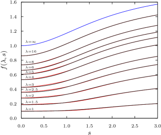
Figure 1: Comparison of enhancement factors,
black: $f(\lambda,s)$ of Eqs. (47) and (49),
red: $\bar{f}(\lambda,s)$ of Eq. (Simple exchange hole models for long-range-corrected density functionals) with $\chi=\chi_{1}$.

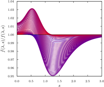
Figure 2: Comparison of enhancement factors:
the ratio $\bar{f}(\lambda,s)/f(\lambda,s)$ as a function of $s$ and $\lambda$.

It is now clear that both kinds of shape functions — both the oscillatory of Eq. (46) and the non-oscillatory of Eq. (57) — would yield nearly the same integral output of Eq. (9) under the same constraints of Eqs. (10), (11), and (12). To our mind, the oscillatory function gives the best solution: we get an explicit closed-form expression for $f(\lambda,s)$ in terms of the given $f(s)$ using Eqs. (18), (49), (50), and (47); furthermore, it has the exact uniform electron gas limit. Nevertheless, our experience with the non-oscillatory functions was not in vain and these can be used in the further work on new functionals.

It might be time for a thorough benchmark of the new model on a wide set of molecules, but we put it off for now until we learn how to combine it with a dispersion-correction functional Dion et al. (2004); Vydrov and van Voorhis (2010).

We find our long-range corrected version of the PBE Perdew et al. (1996) functional with $\frac{1}{\omega}=3\;\mathrm{au}$ (an easy-to-remember whole number) to be already a good next step after its ${\textstyle\frac{1}{4}}$-fixed-fraction hybrid Perdew et al. (1996); Adamo and Barone (1999), and it can be used routinely in mechanistic studies of molecular structure and reactivity toward a full understanding of chemical kinetics.

References

• Langreth and Mehl (1983) D. C. Langreth and M. J. Mehl, “Beyond the local-density approximation in calculations of ground-state electronic properties,” Phys. Rev. B, 28, 1809 (1983).
• Becke (1986) A. D. Becke, “Density functional calculations of molecular bond energies,” J. Chem. Phys., 84, 4524 (1986).
• Perdew and Wang (1986) J. P. Perdew and Y. Wang, “Accurate and simple density functional for the electronic exchange energy: Generalized gradient approximation,” Phys. Rev. B, 33, 8800 (1986).
• Perdew et al. (1996) J. P. Perdew, K. Burke,  and M. Ernzerhof, “Generalized gradient approximation made simple,” Phys. Rev. Lett., 77, 3865 (1996a).
• Hohenberg and Kohn (1964) P. Hohenberg and W. Kohn, “Inhomogeneous electron gas,” Phys. Rev., 136, B864 (1964).
• Kohn and Sham (1965) W. Kohn and L. J. Sham, “Self-consistent equations including exchange and correlation effects,” Phys. Rev., 140, A1133 (1965).
• Becke (1993) A. D. Becke, “A new mixing of hartree–fock and local density‐functional theories,” J. Chem. Phys., 98, 1372 (1993a).
• Becke (1993) A. D. Becke, “Density-functional thermochemistry. iii. the role of exact exchange,” J. Chem. Phys., 98, 5648 (1993b).
• Perdew et al. (1996) J. P. Perdew, M. Ernzerhof,  and K. Burke, “Rationale for mixing exact exchange with density functional approximations,” J. Chem. Phys., 105, 9982 (1996b).
• Iikura et al. (2001) H. Iikura, T. Tsuneda, T. Yanai,  and K. Hirao, “A long-range correction scheme for generalized-gradient-approximation exchange functionals,” J. Chem. Phys., 115, 3540 (2001).
• Gill et al. (1996) P. M. W. Gill, R. D. Adamson,  and J. A. Pople, “Coulomb-attenuated exchange energy density functionals,” Mol. Phys., 88, 1005 (1996).
• Leininger et al. (1997) T. Leininger, H. Stoll, H.-J. Werner,  and A. Savin, “Combining long-range configuration interaction with short-range density functionals,” Chem. Phys. Lett., 275, 151 (1997).
• Tawada et al. (2004) Y. Tawada, T. Tsuneda, S. Yanagisawa, T. Yanai,  and K. Hirao, “A long-range-corrected time-dependent density functional theory,” J. Chem. Phys., 120, 8425 (2004).
• Runge and Gross (1984) E. Runge and E. K. U. Gross, “Density-functional theory for time-dependent systems,” Phys. Rev. Lett., 52, 997 (1984).
• Petersilka et al. (1996) M. Petersilka, U. J. Gossmann,  and E. K. U. Gross, “Excitation energies from time-dependent density-functional theory,” Phys. Rev. Lett., 76, 1212 (1996).
• Dreuw et al. (2003) A. Dreuw, J. L. Weisman,  and M. Head-Gordon, “Long-range charge-transfer excited states in time-dependent density functional theory require non-local exchange,” J. Chem. Phys., 119, 2943 (2003).
• Harris (1984) J. Harris, “Adiabatic-connection approach to kohn-sham theory,” Phys. Rev. A, 29, 1648 (1984).
• Ernzerhof and Perdew (1998) M. Ernzerhof and J. P. Perdew, “Generalized gradient approximation to the angle- and system-averaged exchange hole,” J. Chem. Phys., 109, 3313 (1998).
• Perdew and Wang (1992) J. P. Perdew and Y. Wang, “Pair-distribution function and its coupling-constant average for the spin-polarized electron gas,” Phys. Rev. B, 46, 12947 (1992).
• Heyd et al. (2003) J. Heyd, G. E. Scuseria,  and M. Ernzerhof, “Hybrid functionals based on a screened coulomb potential,” J. Chem. Phys., 118, 8207 (2003).
• Henderson et al. (2008) T. M. Henderson, B. G. Janesko,  and G. E. Scuseria, “Generalized gradient approximation model exchange holes for range-separated hybrids,” J. Chem. Phys., 128, 194105 (2008).
• Rohrdanz et al. (2009) M. A. Rohrdanz, K. M. Martins,  and J. M. Herbert, “A long-range-corrected density functional that performs well for both ground-state properties and time-dependent density functional theory excitation energies, including charge-transfer excited states,” J. Chem. Phys., 130, 054112 (2009).
• Weintraub et al. (2009) E. Weintraub, T. M. Henderson,  and G. E. Scuseria, “Long-range-corrected hybrids based on a new model exchange hole,” J. Chem. Theory Comput., 5, 754 (2009).
• Tao et al. (2017) J. Tao, I. W. Bulik,  and G. E. Scuseria, “Semilocal exchange hole with an application to range-separated density functionals,” Phys. Rev. B, 95, 125115 (2017).
• Becke and Roussel (1989) A. D. Becke and M. R. Roussel, “Exchange holes in inhomogeneous systems: A coordinate-space model,” Phys. Rev. A, 39, 3761 (1989).
• Modrzejewski et al. (2016) M. Modrzejewski, M. Hapka, G. Chalasinski,  and M. M. Szczesniak, “Employing range separation on the meta-gga rung: New functional suitable for both covalent and noncovalent interactions,” J. Chem. Theory Comput., 12, 3662 (2016).
• Tao and Mo (2016) J. Tao and Y. Mo, “Accurate semilocal density functional for condensed-matter physics and quantum chemistry,” Phys. Rev. Lett., 117, 073001 (2016).
• Patra et al. (2018) B. Patra, S. Jana,  and P. Samal, “Long-range corrected density functional through the density matrix expansion based semilocal exchange hole,” Phys. Chem. Chem. Phys., 20, 8991 (2018).
• Negele and Vautherin (1972) J. W. Negele and D. Vautherin, “Density-matrix expansion for an effective nuclear hamiltonian,” Phys. Rev. C, 5, 1472 (1972).
• Koehl et al. (1996) R. M. Koehl, G. K. Odom,  and G. E. Scuseria, “The use of density matrix expansions for calculating molecular exchange energies,” Mol. Phys., 87, 835 (1996).
• Tsuneda and Hirao (2000) T. Tsuneda and K. Hirao, “Parameter-free exchange functional,” Phys. Rev. B, 62, 15527 (2000).
• Becke (1983) A. D. Becke, “Hartree-fock exchange energy of an inhomogeneous electron gas,” Int. J. Quantum Chem., 23, 1915 (1983).
• Perdew et al. (1996) J. P. Perdew, K. Burke,  and Y. Wang, “Generalized gradient approximation for the exchange-correlation hole of a many-electron system,” Phys. Rev. B, 54, 16533 (1996c).
• Becke (1988) A. D. Becke, “Density-functional exchange-energy approximation with correct asymptotic behavior,” Phys. Rev. A, 38, 3098 (1988).
• Hammer et al. (1999) B. Hammer, L. B. Hansen,  and J. K. Nørskov, “Improved adsorption energetics within density-functional theory using revised perdew-burke-ernzerhof functionals,” Phys. Rev. B, 59, 7413 (1999).
• Ma and Brueckner (1968) S.-k. Ma and K. A. Brueckner, “Correlation energy of an electron gas with a slowly varying high density,” Phys. Rev., 165, 18 (1968).
• Lieb and Oxford (1981) E. H. Lieb and S. Oxford, “Improved lower bound on the indirect coulomb energy,” Int. J. Quantum Chem., 19, 427 (1981).
• Lieb (1979) E. H. Lieb, “A lower bound for coulomb energies,” Phys. Lett. A, 70, 444 (1979).
• Adamo and Barone (2002) C. Adamo and V. Barone, “Physically motivated density functionals with improved performances: The modified perdew–burke–ernzerhof model,” J. Chem. Phys., 116, 5933 (2002).
• Campo (2016) J. M. d. Campo, “B88 exchange functional recovering the local spin density linear response,” Theor. Chem. Acc., 135 (2016), doi:10.1007/s00214-016-1929-2.
• Jaynes (1957) E. T. Jaynes, “Information theory and statistical mechanics,” Phys. Rev., 106, 620 (1957).
• Dion et al. (2004) M. Dion, H. Rydberg, E. Schröder, D. C. Langreth,  and B. I. Lundqvist, “Van der waals density functional for general geometries,” Phys. Rev. Lett., 92, 246401 (2004).
• Vydrov and van Voorhis (2010) O. A. Vydrov and T. van Voorhis, “Nonlocal van der waals density functional: The simpler the better,” J. Chem. Phys., 133, 244103 (2010).
• Adamo and Barone (1999) C. Adamo and V. Barone, “Toward reliable density functional methods without adjustable parameters: The pbe0 model,” J. Chem. Phys., 110, 6158 (1999).