High-order ALE gas-kinetic scheme with unstructured WENO reconstruction

Abstract

In this paper, a high-order multi-dimensional gas-kinetic scheme is presented for both inviscid and viscous flows in arbitrary Lagrangian-Eulerian (ALE) formulation. Compared with the traditional ALE method, the flow variables are updated in the finite volume framework, and the rezoning and remapping steps are not required. The two-stage fourth-order method is used for the temporal discretization, and the second-order gas-kinetic solver is applied for the flux evaluation. In the two-stage method, the spatial reconstruction is performed at both initial and intermediate stage, and the computational mesh at the corresponding stage is given by the specified mesh velocity. In the moving mesh procedure, the mesh may distort severely and the mesh quality is reduced. To achieve the accuracy and improve the robustness, the newly developed WENO method [41] on quadrilateral unstructured meshes is adopted at each stage. The Gaussian quadrature is used for flux calculation. For each Gaussian point, the reconstruction performed in the local moving coordinate, where the variation of mesh velocity is taken into account. Therefore, the accuracy and geometric conservation law can be well preserved by the current scheme even with the largely deforming mesh. Numerical examples are presented to validate the performance of current scheme, where the mesh adaptation method and cell centered Lagrangian method are used to provide mesh velocity.

1 Introduction

In the computational fluid dynamics, there exist two coordinate systems to describe flow motions, where the Eulerian system describes flow motions with time-independent mesh and the mesh moves with the fluid velocity in the Lagrangian system. Considerable progress has been made over the past decades for the numerical simulations based on these two descriptions [2, 25, 36]. The Eulerian system is relatively simple, but it smears contact discontinuities and slip lines badly. For the computation with fixed boundaries, the Eulerian system could work effectively. However, in the problems with moving boundaries and bodies, it becomes difficult for the Eulerian method. On the other hand, the Lagrangian system could resolve contact discontinuities sharply, but computation can easily break down due to mesh deformation. In order to avoid mesh distortion and tangling in the Lagrangian method, a widely used arbitrary-Lagrangian-Eulerian (ALE) technique was developed [15], which contains three main steps. In the Lagrangian stage, the solution and the computational mesh are updated simultaneously. To release the error due to mesh deformation, the computational mesh is adjusted to the optimal position in the rezoning stage. In the remapping stage, the Lagrangian solution is transferred into the rezoned mesh. Further developments and great achievement have been made for the ALE method [1, 21, 11, 37].

In the past decades, the gas-kinetic scheme (GKS) based on the Bhatnagar-Gross-Krook (BGK) model [3, 6] has been developed systematically for computations from low speed flow to supersonic one [39, 40]. Different from the numerical methods based on the Riemann flux [36], GKS presents a gas evolution process from kinetic scale to hydrodynamic scale, where both inviscid and viscous fluxes are recovered from a time-dependent and multi-dimensional gas distribution function at a cell interface. Recently, based on the time-dependent flux function of the generalized Riemann problem (GRP) [4, 5] and gas-kinetic scheme, a two-stage fourth-order method was developed for Lax-Wendroff type flow solvers, particularly applied for the hyperbolic conservation laws [24, 10, 27, 28, 29]. Under the multi-stage multi-derivative framework, a reliable two-stage fourth-order GKS has been developed, and even higher-order of accuracy can be achieved. More importantly, this scheme is as robust as the second-order scheme and works perfectly from subsonic to hypersonic flows. Based on the unified coordinate transformation [13], the second-order gas-kinetic scheme was developed under the moving-mesh framework [16, 17]. With the integral form of the fluid dynamic equations, a second-order gas-kinetic scheme with arbitrary mesh velocity was developed [26], in which the rezoning and remapping step in the traditional ALE method is avoided. It provides a general framework for the moving-mesh method, which can be considered as a remapping-free ALE-type method. The piecewise constant mesh velocity at each cell interface is considered in the ALE-type gas-kinetic scheme, which is reasonable for a second-order scheme. However, for the higher-order schemes, the variation of the mesh velocity along a cell interface needs to be taken into account. Otherwise, the geometric conservation law may be violated during the mesh rotating and deformation. Recently, a one-stage DG-ALE gas-kinetic method was developed, especially for the oscillating airfoil calculations [31]. The variation of mesh velocity is considered in the time dependent flux calculation along a cell interface, and the geometric conservation law can be satisfied accurately. However, the one-stage gas evolution model and DG framework become very complicated, and the efficiency of the DG-ALE-GKS becomes low due to the severely constrained time step from the DG formulation.

In this paper, a robust WENO scheme [41], which was developed recently on unstructured quadrilateral meshes, is extended into the gas-kinetic framework. The optimization approach for linear weights and the non-linear weights with new smooth indicator improves the robustness of traditional WENO scheme. With the arbitrary Lagrangian-Eulerian formulation, a high-order moving-mesh gas-kinetic scheme is developed for the inviscid and viscous flows. It extends the gas-kinetic scheme with unstructured WENO reconstruction from the static domain to the variable one. The two-stage fourth-order method is used for the temporal discretization, in which the computational mesh at the corresponding stage is given by the specified mesh velocity, and the WENO reconstruction is performed at the initial and intermediate stage respectively. The mesh velocity inside each cell interface are considered and the WENO reconstruction is performed at each Gaussian quadrature point in the local moving coordinate. Thus, the accuracy and geometric conservation law can be well preserved by the current scheme even with the largely deforming mesh. Numerical examples are presented to validate the performance of current scheme, where the mesh adaptation method and cell centered Lagrangian method are used to provide the mesh velocity.

This paper is organized as follows. In Section 2, the gas-kinetic scheme on moving-mesh is introduced. The extension of the two-stage temporal discretization to moving mesh system is presented in Section 3. In Section 4, we give the WENO reconstruction on unstructured quadrilateral meshes. Section 5 includes numerical examples to validate the current algorithm. The last section is the conclusion.

2 Gas-kinetic scheme on moving-meshes

The two-dimensional BGK equation can be written as [3, 6],

$$f_{t}+uf_{x}+vf_{y}=\frac{g-f}{\tau},$$ (1)

where $f$ is the gas distribution function, $g$ is the corresponding equilibrium state, and $\tau$ is the collision time. The collision term satisfies the compatibility condition

$$\int\frac{g-f}{\tau}\psi\text{d}\Xi=0,$$ (2)

where $\psi=(1,u,v,\displaystyle\frac{1}{2}(u^{2}+v^{2}+\xi^{2}))$, $\text{d}\Xi=\text{d}u\text{d}v\text{d}\xi^{1}...\text{d}\xi^{K}$, $K$ is the number of internal degrees of freedom, i.e. $K=(4-2\gamma)/(\gamma-1)$ for two-dimensional flows, and $\gamma$ is the specific heat ratio. In the continuum regime, the gas distribution function can be expanded as

$$f=g-\tau D_{\bm{u}}g+\tau D_{\bm{u}}(\tau D_{\bm{u}})g-\tau D_{\bm{u}}[\tau D_{\bm{u}}(\tau D_{\bm{u}})g]+...,$$

where $D_{\bm{u}}={\partial}/{\partial t}+\bm{u}\cdot\nabla$. With the zeroth order truncation, i.e. $f=g$, the Euler equations can be obtained. For the Navier-Stokes equations, the first order truncation is used

$$f=g-\tau(ug_{x}+vg_{y}+g_{t}).$$

With the higher order truncations, the Burnett and super-Burnett equations can be obtained [39, 40].

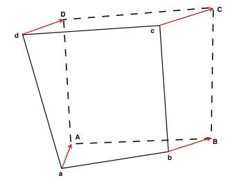
Figure 1: Schematic for moving control volume: $\Omega(t)$ moves from $[abcd]$ at $t^{n}$ to $[ABCD]$ at $t^{n+1}$.

In this paper, the high-order ALE gas-kinetic scheme will be constructed in the moving-mesh framework. As shown in Fig.1, a quadrilateral cell $\Omega(t)$ moves from $[abcd]$ at $t^{n}$ to $[ABCD]$ at $t^{n+1}$ with grid velocity $\bm{U}^{g}=(U^{g},V^{g})$, which varies along each segment. The boundary is given by

$$\partial\Omega_{i}(t)=\bigcup_{m}\Gamma_{im}(t),$$

where $\Gamma_{im}(t)$ is the line segment of boundary. For simplicity, the mesh velocity is set to be constant during a time interval, and the segments keep straight in a time step. Standing on the moving reference, the BGK equation Eq.(1) becomes

$$f_{t}+(u-U^{g})f_{x}+(v-V^{g})f_{y}=\frac{g-f}{\tau}.$$ (3)

Taking moments of the kinetic equation Eq.(3) and integrating with respect to space, the finite volume scheme can be expressed as

$$\frac{\text{d}(|\Omega_{i}|W_{i})}{\text{d}t}=-\sum_{m}F_{im}(t),$$ (4)

where $W_{i}$ is the cell averaged conservative value of $\Omega_{i}$, $|\Omega_{i}|$ is the area of $\Omega_{i}$ and $F_{im}(t)$ is the time dependent fluxes across cell interface $\Gamma_{im}$, which is a line integral over $\Gamma_{im}$

$$F_{im}(t)= \int_{\Gamma_{im}}(\int\psi f(\bm{x}(s),t,\bm{u},\xi)(\bm{u}-\bm{U}^{g})\cdot\bm{n}_{im}\text{d}\Xi)\text{d}s,$$

where $f(\bm{x}(s),t,\bm{u},\xi)$ is the gas distribution function in the global coordinate and $\bm{n}_{im}=(L_{im},M_{im})$ is the outer normal direction of $\Gamma_{im}$. To simplify the calculation, the Gaussian quadrature is used for flux calculation

$$F_{im}(t)=|\Gamma_{im}|\sum_{p}\omega_{i,m_{p}}F_{i,m_{p}}(t).$$

The flux at the Gaussian quadrature points is defined as

$$F_{i,m_{p}}(t)=\left(\begin{array}[]{c}F^{\rho}_{i,m_{p}}\\ F^{m}_{i,m_{p}}\\ F^{n}_{i,m_{p}}\\ F^{E}_{i,m_{p}}\\ \end{array}\right)=\int\psi f(\bm{x}_{i,m_{p}},t,\bm{u},\xi)(\bm{u}-\bm{U}_{i,m_{p}}^{g})\cdot\bm{n}_{im}\text{d}\Xi,$$

where $\bm{x}_{i,m_{p}}$ is the Gaussian quadrature point of $\Gamma_{im}$, $\omega_{i,m_{p}}$ is the quadrature weight and $\bm{U}_{i,m_{p}}^{g}$ is the grid velocity at quadrature point. With the Gaussian quadrature, the high-order spatial accuracy is achieved, and the grid velocity variation along a cell interface is considered, in which the translation, rotation and deformation are taken into account. With identified normal direction, the relative particle velocity at the Gaussian point in the local coordinate is defined as

$$\begin{cases}\widetilde{u}=(u-U_{i,m_{p}}^{g})L_{im}+(v-V_{i,m_{p}}^{g})M_{im},\\ \widetilde{v}=-(u-U_{i,m_{p}}^{g})M_{im}+(v-V_{i,m_{p}}^{g})L_{im}.\end{cases}$$ (5)

In the actual computation, the spatial reconstruction, which will be presented in the later section, is performed in a local moving coordinate. With the reconstructed variables, the gas distribution function is obtained at Gaussian quadrature point. The numerical flux can be obtained by taking moments of it, and the component-wise form can be written as

$$\widetilde{F}_{i,m_{p}}(t)=\left(\begin{array}[]{c}F^{\widetilde{\rho}}_{i,m_{p}}\\ F^{\widetilde{m}}_{i,m_{p}}\\ F^{\widetilde{n}}_{i,m_{p}}\\ F^{\widetilde{E}}_{i,m_{p}}\\ \end{array}\right)=\int\widetilde{u}\left(\begin{array}[]{c}1\\ \widetilde{u}\\ \widetilde{v}\\ \frac{1}{2}(\widetilde{u}^{2}+\widetilde{v}^{2}+\xi^{2})\\ \end{array}\right)f(\bm{x}_{i,m_{p}},t,\widetilde{\bm{u}},\xi)\text{d}\widetilde{\Xi},$$

where $f(\bm{x}_{i,m_{p}},t,\widetilde{\bm{u}},\xi)$ is the gas distribution function in the local coordinate. According to Eq.(5), the fluxes in the inertia frame of reference can be obtained as a combination of the fluxes in the moving frame of reference

$$\left\{\begin{aligned} F^{\rho}_{i,m_{p}}=&F^{\widetilde{\rho}}_{i,m_{p}},\\ F^{m}_{i,m_{p}}=&\big{(}U_{i,m_{p}}^{g}F^{\widetilde{\rho}}_{i,m_{p}}+M_{im}F^{\widetilde{m}}_{i,m_{p}}+L_{im}F^{\widetilde{n}}_{i,m_{p}}\big{)},\\ F^{n}_{i,m_{p}}=&\big{(}V_{i,m_{p}}^{g}F^{\widetilde{\rho}}_{i,m_{p}}-L_{im}F^{\widetilde{m}}_{i,m_{p}}+M_{im}F^{\widetilde{n}}_{i,m_{p}}\big{)},\\ F^{E}_{i,m_{p}}=&\big{(}F^{\widetilde{E}}_{i,m_{p}}+\frac{1}{2}((U_{i,m_{p}}^{g})^{2}+(V_{i,m_{p}}^{g})^{2})F^{\widetilde{\rho}}_{i,m_{p}}\\ &+(M_{im}U_{i,m_{p}}^{g}-L_{im}V_{i,m_{p}}^{g})F^{\widetilde{m}}_{i,m_{p}}+(L_{im}U_{i,m_{p}}^{g}+M_{im}V_{i,m_{p}}^{g})F^{\widetilde{n}}_{i,m_{p}}\big{)}.\end{aligned}\right.$$ (6)

To construct the gas distribution function in the local coordinate, the integral solution of the BGK equation at a cell interface is used

$$f(\bm{x}_{i,m_{p}},t,\bm{u},\xi)=\frac{1}{\tau}\int_{0}^{t}g(x^{\prime},y^{\prime},t^{\prime},u,v,\xi)e^{-(t-t^{\prime})/\tau}\text{d}t^{\prime}\\ +e^{-t/\tau}f_{0}(-ut,-vt,u,v,\xi),$$ (7)

where $\widetilde{\bm{u}}$ is simply denoted as $\bm{u}$, $\bm{x}_{i,m_{p}}=(x_{i,m_{p}},y_{i,m_{p}})$ is the location of Gaussian quadrature point, $x_{i,m_{p}}=x^{\prime}+u(t-t^{\prime}),y_{i,m_{p}}=y^{\prime}+v(t-t^{\prime})$ are the trajectory of particles, $f_{0}$ is the initial gas distribution function, and $g$ is the corresponding equilibrium state. According to Eq.(7), the time dependent gas distribution function $f(\bm{x}_{i,m_{p}},t,\bm{u},\xi)$ at the cell interface can be expressed as [40, 39]

$$f(\bm{x}_{i,m_{p}},t,\bm{u},\xi)= (1-e^{-t/\tau})g_{0}+((t+\tau)e^{-t/\tau}-\tau)(\overline{a}_{1}u+\overline{a}_{2}v)g_{0}$$

$$+ (t-\tau+\tau e^{-t/\tau}){\bar{A}}g_{0}$$

$$+ e^{-t/\tau}g_{r}[1-(\tau+t)(a_{1r}u+a_{2r}v)-\tau A_{r})]H(u)$$

$$+ e^{-t/\tau}g_{l}[1-(\tau+t)(a_{1l}u+a_{2l}v)-\tau A_{l})](1-H(u)),$$ (8)

where the coefficients in Eq.(2) can be determined by the reconstructed directional derivatives and compatibility condition

$$\displaystyle\langle a_{1}^{k}\rangle=\frac{\partial W_{k}}{\partial\bm{n}},\langle a_{2}^{k}\rangle =\frac{\partial W_{k}}{\partial\bm{\tau}},\langle a_{1}^{k}u+a_{2}^{k}v+A^{k}\rangle=0,$$

$$\displaystyle\langle\overline{a}_{1}\rangle=\frac{\partial\overline{W}}{\partial\bm{n}},\langle\overline{a}_{2}\rangle =\frac{\partial\overline{W}}{\partial\bm{\tau}},\langle\overline{a}_{1}u+\overline{a}_{2}v+\overline{A}\rangle=0,$$

where $k=l,r$, $\bm{n}$ and $\bm{\tau}$ are local normal and tangential direction and $\langle...\rangle$ are the moments of the equilibrium $g$ and defined by

$$\langle...\rangle=\int g(...)\psi\text{d}\Xi.$$

The spatial derivatives will be obtained by the WENO reconstruction, which will be given later. More details of the gas-kinetic scheme can be found in [39].

In the formulations above, the grid velocity $\bm{U}^{g}$ can be arbitrary to control the volume evolution. The Eulerian governing equation is obtained with $\bm{U}^{g}=0$, and the Lagrangian form is obtained with $\bm{U}^{g}=\bm{U}$, where $\bm{U}$ is the fluid velocity. In this paper, the structured meshes are used in the moving mesh computation for simplicity, while the unstructured reconstruction is used to deal with the distorted meshes. The strategies of mesh velocity are given as follows

1. The mesh velocity is specified directly. This is the simplest type of mesh velocity and is mainly adopted in the accuracy tests in this paper.

2. The mesh velocity can be given by the fluid velocity, and the cell centered Lagrangian nodal solver is used [25]. Denote $\bm{U}_{p}$ as the vertex fluid velocity of the control volume, $\bm{U}_{c}$ as cell averaged fluid velocity, $C(p)$ as the set of control volumes that share the common vertex $p$, the mesh velocity can be obtained by solving the following linear system

   $$\sum_{c\in C(p)}\mathbb{M}_{pc}\bm{U}_{p}=\sum_{c\in C(p)}l_{pc}p_{c}\bm{n}_{pc}+\mathbb{M}_{pc}\bm{U}_{c},$$

   where

   $$\mathbb{M}_{pc}=\rho_{c} a_{c}[l_{pc}^{-}(\bm{n}_{pc}^{-}\otimes\bm{n}_{pc}^{-})+l_{pc}^{+}(\bm{n}_{pc}^{+}\otimes\bm{n}_{pc}^{+})],$$

   $$l_{pc}\bm{n}_{pc}=l_{pc}^{-}\bm{n}_{pc}^{-}+l_{pc}^{+}\bm{n}_{pc}^{+},$$

   where $pp^{-}$ and $pp^{+}$ are the line segments of $c$ that share the vertex $p$. $l_{pc}^{-},l_{pc}^{+}$ and $\bm{n}_{pc}^{-},\bm{n}_{pc}^{+}$ are the half lengthes and outer normal directions of the two segments. The matrix $\mathbb{M}_{pc}$ is symmetric positive definite. Therefore, the system will always admit a unique solution.

3. The mesh velocity can be determined by the variational approach [34], and the corresponding Euler-Lagrange equations can be obtained from

   $$(\omega x_{\xi})_{\xi} +(\omega x_{\eta})_{\eta}=0,$$

   $$(\omega y_{\xi})_{\xi} +(\omega y_{\eta})_{\eta}=0,$$

   where $(x,y)$ and $(\xi,\eta)$ denote the physical and computational coordinates, $\omega$ is the monitor function and can be chosen as a function of the flow variables, such as the density, velocity, pressure, or their gradients. In the numerical tests, the monitor function takes the form

   $$\omega=\sqrt{1+\alpha|\nabla\rho|^{2}},$$

   if no special statement is given. The mesh distribution in the physical space can be directly generated [34].

In order to avoid mesh distortion, the new meshes obtained by the Lagrangian method and adaption method are smoothed by the following smooth procedure for the structured meshes

$$\widetilde{\bm{x}}^{n+1}_{ij}= (4\bm{x}^{n+1}_{ij}+\bm{x}^{n+1}_{i-1,j}+\bm{x}^{n+1}_{i+1,j}+\bm{x}^{n+1}_{i,j-1}+\bm{x}^{n+1}_{i,j+1})/8,$$

where $\bm{x}_{ij}$ is the coordinate of the grid points. This procedure is conducted for some certain steps. The velocity at grid points $\textbf{U}_{ij}^{g}=(U_{ij}^{g},V_{ij}^{g})$ can be determined as follows

$$\bm{U}_{ij}^{g}=\frac{\widetilde{\bm{x}}^{n+1}_{ij}-\bm{x}^{n}_{ij}}{\Delta t}.$$

The mesh velocity $\bm{U}_{i,j_{p}}^{g}$ and $\bm{U}_{i_{p},j}^{g}$ at Gaussian quadrature points can be obtained by the linear interpolation of mesh velocity at the grid points.

3 Two-stage temporal discretization

A two-stage fourth-order time-accurate discretization was developed for Lax-Wendroff flow solvers, such as the generalized Riemann problem (GRP) solver and the gas-kinetic scheme [23]. Consider the following time-dependent equation

$$\frac{\partial\bm{w}}{\partial t}=\mathcal{L}(\bm{w}),$$ (9)

with the initial condition at $t_{n}$, i.e.,

$$\bm{w}(t=t_{n})=\bm{w}^{n},$$

where $\mathcal{L}$ is an operator for spatial derivative of flux. Introducing an intermediate state at $t^{*}=t_{n}+\Delta t/2$,

$$\bm{w}^{*}=\bm{w}^{n}+\frac{1}{2}\Delta t\mathcal{L}(\bm{w}^{n})+\frac{1}{8}\Delta t^{2}\frac{\partial}{\partial t}\mathcal{L}(\bm{w}^{n}),$$ (10)

the state $\bm{w}$ can be updated with the following formula

$$\bm{w}^{n+1}=\bm{w}^{n}+\Delta t\mathcal{L}(\bm{w}^{n})+\frac{1}{6}\Delta t^{2}\big{(}\frac{\partial}{\partial t}\mathcal{L}(\bm{w}^{n})+2\frac{\partial}{\partial t}\mathcal{L}(\bm{w}^{*})\big{)}.$$ (11)

It can be proved that Eq.(10) and Eq.(11) provide a fourth-order time accurate solution for Eq.(9) at $t=t_{n}+\Delta t$. The details of proof can be found in [24].

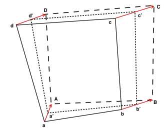
Figure 2: Schematic for a moving control volume: $\Omega(t^{*})=[a^{\prime}b^{\prime}c^{\prime}d^{\prime}]$ is the intermediate one at $t^{*}=t_{n}+\Delta t/2$ and $a^{\prime},b^{\prime},c^{\prime},d^{\prime}$ are the mid-points of $aA,bB,cC,dD$.

To achieve the high-order spatial and temporal accuracy, the two-stage temporal discretization can be extended to the moving mesh computation Eq.(4), where the operator $\mathcal{L}$ is denoted as

$$\mathcal{L}(\Omega_{i},W_{i})=-\sum_{m}F_{im}(t).$$

As shown in Fig.2, the coordinate of the local moving reference and the length of cell interface are both time-dependent, which is critical for accuracy and geometry conservation law. In the two-stage method, the variables are defined and the reconstruction is performed at $t_{n}$ and $t^{*}=t_{n}+\Delta t/2$, respectively. Due to the constant velocity for each vertex, the intermediate control volume at $t^{*}$ moves to $\Omega(t^{*})=[a^{\prime}b^{\prime}c^{\prime}d^{\prime}]$ exactly, where $a^{\prime},b^{\prime},c^{\prime},d^{\prime}$ are the mid-points of $aA,bB,cC,dD$. To implement the two-stage method, the WENO reconstructions is performed with the re-distributed meshes at $t_{n}$ and $t^{*}$. With the reconstructed variables, $\mathcal{L}(W)$ and temporal derivative $\partial_{t}\mathcal{L}(W)$ for $\Omega_{i}$ at $t_{n}$ can be written as

$$\mathcal{L}(\Omega_{i}^{n},W_{i}^{n}) =-\sum_{m}\sum_{p}\omega_{m_{p}}|\Gamma_{im}^{n}|\cdot F_{i,m_{p}}^{n},$$

$$\partial_{t}\mathcal{L}(\Omega_{i}^{n},W_{i}^{n}) =-\sum_{m}\sum_{p}\omega_{m_{p}}|\Gamma_{im}^{n}|\cdot\partial_{t}F_{i,m_{p}}^{n},$$

where the coefficient $F_{i,m_{p}}^{n}$ and $\partial_{t}F_{i,m_{p}}^{n}$ can be given by the linear combination of $\widetilde{F}_{i,m_{p}}^{n}$ and $\partial_{t}\widetilde{F}_{i,m_{p}}^{n}$, which are the coefficients of linear approximation of the time dependent flux in the local coordinate

$$\widetilde{F}_{i,m_{p}}(t)=\widetilde{F}_{i,m_{p}}^{n}+\partial_{t}\widetilde{F}_{i,m_{p}}^{n}(t-t_{n}).$$ (12)

To implement two-stage method, the following notation is introduced

$$\widehat{\mathbb{F}}(\bm{x}_{i,m_{p}},\delta)=\int_{t_{n}}^{t_{n}+\delta}\widetilde{F}_{i,m_{p}}(t)\text{d}t=\int_{t_{n}}^{t_{n}+\delta}\int\widetilde{u}\widetilde{\psi}f(\bm{x}_{i,m_{p}},t,\widetilde{\bm{u}},\xi)\text{d}\Xi\text{d}t.$$

Integrating Eq.(12) over $[t_{n},t_{n}+\Delta t/2]$ and $[t_{n},t_{n}+\Delta t]$, we have the following two equations

$$\widetilde{F}_{i,m_{p}}^{n}\Delta t +\frac{1}{2}\partial_{t}\widetilde{F}_{i,m_{p}}^{n}\Delta t^{2}=\widehat{\mathbb{F}}(\bm{x}_{i,m_{p}},\Delta t),$$

$$\frac{1}{2}\widetilde{F}_{i,m_{p}}^{n}\Delta t +\frac{1}{8}\partial_{t}\widetilde{F}_{i,m_{p}}^{n}\Delta t^{2}=\widehat{\mathbb{F}}(\bm{x}_{i,m_{p}},\Delta t/2).$$

The coefficients $\widetilde{F}_{i,m_{p}}^{n}$ and $\partial_{t}\widetilde{F}_{i,m_{p}}^{n}$ can be determined by solving the linear system. Similarly, $\mathcal{L}(\Omega_{i}^{*},W_{i}^{*})$ and temporal derivative $\partial_{t}\mathcal{L}(\Omega_{i}^{*},W_{i}^{*})$ at the intermediate state can be constructed as well. According to Eq.(6), the coefficients $F_{i,m_{p}}^{n}$ and $\partial_{t}F_{i,m_{p}}^{n}$ in the global coordinate can be obtained. More details of the two-stage fourth-order scheme can be found in [24, 27].

4 Unstructured WENO reconstruction

During the moving-mesh procedure, the mesh becomes distorted and the development of robust high-order scheme on a low quality mesh is demanding. Recently, a third-order WENO reconstruction is constructed on quadrilateral and triangular meshes [41], in which high-order accuracy is achieved and robustness is improved. In this section, the third-order WENO reconstruction is extended to the framework of gas-kinetic scheme. For the moving-mesh computation, the spatial reconstruction is performed in the local moving coordinate at each Gaussian quadrature point, where the variation of mesh velocity is considered along a cell interface.

Figure 3: Stencils for third-order schemes on quadrilateral meshes.

In this section, the reconstruction on quadrilateral mesh is reviewed briefly and more details can be found in [41]. To improve the robustness of WENO scheme, a general selection of stencils is given as shown in Fig.4. To achieve the third-order accuracy, the following quadratic polynomial $P^{2}(x,y)$ can be constructed

$$P^{2}(x,y)=W_{i_{0}}+\sum_{k=1}^{5}a_{k}p^{k}(x,y),$$ (13)

where $W_{i_{0}}$ is the cell average value of $W(x,y)$ over cell $\Omega_{i_{0}}$ and $p^{k}(x,y),k=1,...,5$ are basis functions, which are given as follows

$$\begin{cases}\displaystyle p^{1}(x,y)=x-\frac{1}{\left|\Omega_{i_{0}}\right|}\displaystyle\iint_{\Omega_{i_{0}}}x\text{d}x\text{d}y,\\ \displaystyle p^{2}(x,y)=y-\frac{1}{\left|\Omega_{i_{0}}\right|}\displaystyle\iint_{\Omega_{i_{0}}}y\text{d}x\text{d}y,\\ \displaystyle p^{3}(x,y)=x^{2}-\frac{1}{\left|\Omega_{i_{0}}\right|}\displaystyle\iint_{\Omega_{i_{0}}}x^{2}\text{d}x\text{d}y,\\ \displaystyle p^{4}(x,y)=y^{2}-\frac{1}{\left|\Omega_{i_{0}}\right|}\displaystyle\iint_{\Omega_{i_{0}}}y^{2}\text{d}x\text{d}y,\\ \displaystyle p^{5}(x,y)=xy-\frac{1}{\left|\Omega_{i_{0}}\right|}\displaystyle\iint_{\Omega_{i_{0}}}xydxdy.\end{cases}$$ (14)

With the following constraint over the cell $\Omega_{i_{j}},i_{j}\in S=\{i_{0},i_{1},...,i_{12}\}$,

$$\frac{1}{\left|\Omega_{i_{j}}\right|}\int_{\Omega_{i_{j}}}P^{2}(x,y)\text{d}x\text{d}y=W_{i_{j}},$$

the coefficients $\textbf{a}=(a_{1},...,a_{5})$ in Eq.(13) can be fully given, where $W_{i_{j}}$ is the cell averaged variables over cell $\Omega_{i_{j}}$ .

Similar with the standard WENO reconstruction [14], twelve sub-stencils $S_{j},j=1,...,12$ are selected from the large stencil given in Fig.4

$$P_{1}^{1}~{} \text{on}~{}S_{1}=\{i_{0},i_{1},i_{2}\},~{}~{}~{}P_{2}^{1}~{}\text{on}~{}S_{2}=\{i_{0},i_{2},i_{3}\},~{}~{}~{}P_{3}^{1}~{}\text{on}~{}S_{3}=\{i_{0},i_{3},i_{4}\},$$

$$P_{4}^{1}~{} \text{on}~{}S_{4}=\{i_{0},i_{4},i_{1}\},~{}~{}~{}P_{5}^{1}~{}\text{on}~{}S_{5}=\{i_{0},i_{1},i_{5}\},~{}~{}~{}P_{6}^{1}~{}\text{on}~{}S_{6}=\{i_{0},i_{1},i_{6}\},$$

$$P_{7}^{1}~{} \text{on}~{}S_{7}=\{i_{0},i_{3},i_{7}\},~{}~{}~{}P_{8}^{1}~{}\text{on}~{}S_{8}=\{i_{0},i_{3},i_{8}\},~{}~{}~{}P_{9}^{1}~{}\text{on}~{}S_{9}=\{i_{0},i_{4},i_{9}\},$$

$$P_{10}^{1}~{} \text{on}~{}S_{10}=\{i_{0},i_{2},i_{10}\},P_{11}^{1}~{}\text{on}~{}S_{11}=\{i_{0},i_{2},i_{11}\},P_{12}^{1}~{}\text{on}~{}S_{12}=\{i_{0},i_{4},i_{12}\}.$$

Twelve candidate linear polynomials $P_{j}^{1}$ corresponding to the candidate sub-stencils can be constructed as follows

$$\frac{1}{\left|\Omega_{S_{j,k}}\right|}\int_{\Omega_{S_{j,k}}}P^{1}_{j}(x,y)\text{d}x\text{d}y=W_{S_{j,k}},~{}k=0,1,2,$$

where $\Omega_{S_{j,k}}$ is the $(k+1)$-th cell in the sub-stencils $S_{j}$, and $W_{S_{j,k}}$ is the cell averaged value over cell $\Omega_{S_{j,k}}$.

With point value of the quadratic polynomial $P^{2}(x,y)$ and linear polynomials $P_{j}^{1}$ at the Gaussian quadrature point $(x_{G},y_{G})$, a standard procedure of WENO scheme is adopted to obtain the linear weights $\gamma_{j}$ [14]. However, in the traditional WENO reconstruction, the very large linear weights and negative weights appear with the lower mesh quality. In order to improve the robustness of WENO schemes, an optimization approach is given to deal with the very large linear weights. The weighting parameters is introduced for each cell, such that the ill cell contributes little to the quadratic polynomial in Eq.(13). For quadrilateral meshes, the weighting parameters are defined for each cell

$$\begin{cases}d_{j}=1,&~{}~{}j=1,...,4,\\ d_{j}=\displaystyle\frac{1}{\max(1,\left|\gamma_{j}\right|)},&~{}~{}j=5,...,12.\end{cases}$$

The optimized coefficients $\textbf{a}=(a_{1},...,a_{5})$ of the quadratic polynomial in Eq.(13) are given by the following weighted linear system

$$\sum_{k=1}^{5}d_{j}\cdot A_{jk}a_{k}=d_{j}\cdot(W_{i_{j}}-W_{i_{0}}).$$

With the procedure above, the maximum $\gamma_{j}$ becomes the order $O(1)$ [41].

To deal with the negative linear weights, the splitting technique [32] is considered for the optimized approach as follows

$$\widetilde{\gamma}_{j}^{+}=\frac{1}{2}(\gamma_{j}+\theta\left|\gamma_{j}\right|),~{}~{}\widetilde{\gamma}_{j}^{-}=\widetilde{\gamma}_{j}^{+}-\gamma_{j},$$

where $\theta=3$ is taken in numerical tests. The scaled non-negative linear weights $\gamma_{j}^{\pm}$ and nonlinear weights $\delta_{j}^{\pm}$ are given by

$$\gamma_{j}^{\pm}=\frac{\widetilde{\gamma}_{j}^{\pm}}{\sigma^{\pm}}, ~{}\sigma^{\pm}=\sum_{j}\widetilde{\gamma}_{j}^{\pm},$$

$$\delta_{j}^{\pm}=\frac{\alpha_{j}^{\pm}}{\sum_{l=1}\alpha_{l}^{\pm}}, ~{}~{}\alpha_{j}^{\pm}=\frac{\gamma_{j}^{\pm}}{(\widetilde{\beta}_{j}^{\pm}+\epsilon)^{2}},$$

where $\epsilon$ is a small positive number, $\widetilde{\beta_{j}}^{\pm}$ is a new smooth indicator defined on unstructured meshes

$$\widetilde{\beta_{j}}^{\pm}=\beta_{j}\big{(}1+\gamma_{j}^{\pm}\beta_{j}+(\gamma_{j}^{\pm}\beta_{j})^{2}\big{)},$$

where $\beta_{j}$ is defined as

$$\beta_{j}=\sum_{|\alpha|=1}^{K}|\Omega|^{|\alpha|-1}\iint_{\Omega}\big{(}D^{\alpha}P_{j}^{1}(x,y)\big{)}^{2}\text{d}x\text{d}y,$$

$\alpha$ is a multi-index, and $D$ is the derivative operator. With the new smooth indicator, the accuracy keeps the original order in smooth regions with $IS=h^{2}(1+O(h))$. The final reconstructed value at the Gaussian quadrature points can be written as

$$R(x_{G},y_{G})=\sum_{j}(\delta_{j}^{+}P^{1}_{j}(x_{G},y_{G})-\delta_{j}^{-}P^{1}_{j}(x_{G},y_{G})).$$

Compared with the numerical scheme based on the Riemann solvers, the reconstruction corresponding equilibrium state is also presented. With the reconstructed variables $W_{l}$ and $W_{r}$ at both sides of the cell interface, the variables at the cell interface can be determined by the compatibility condition Eq.(2) as follows

$$\int\psi g_{G}\text{d}\Xi=W_{G}=\int_{u>0}\psi g_{l}\text{d}\Xi+\int_{u<0}\psi g_{r}\text{d}\Xi,$$

where $g_{l}$ and $g_{r}$ are the equilibrium states corresponding to $W_{l}$ and $W_{r}$ respectively. To third-order accuracy, the Taylor expansion corresponding to equilibrium state at the center of cell interface is expressed as

$$\overline{W}(x,y)=W_{G}+\overline{W}_{\bm{n}}(x-x_{G})+\overline{W}_{\bm{\tau}}(y-y_{G})$$

$$+\frac{1}{2}\overline{W}_{\bm{n}\bm{n}} (x-x_{G})^{2}+\overline{W}_{\bm{n}\bm{\tau}}(x-x_{G})(y-y_{G})+\frac{1}{2}\overline{W}_{\bm{\tau}\bm{\tau}}(y-y_{G})^{2},$$

where $\bm{n},\bm{\tau}$ are local normal and tangential directions. With the following constrains

$$\frac{1}{\left|\Omega_{i_{j}}\right|}\int_{\Omega_{i_{j}}}\overline{W}(x,y)\text{d}x\text{d}y=W_{i_{j}},i_{j}\in T=\{i_{0},i_{1},...,i_{7}\},$$

the spatial derivatives can be obtained by the least square methods, where the stencils for equilibrium state reconstruction is given in Fig.4. For most mesh generation method, there are at least five elements in the above stencil, which guarantees the least square method solvable.

Figure 4: Stencils for equilibrium state of third-order scheme on quadrilateral meshes.

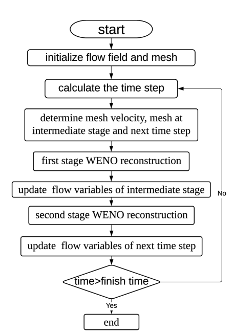
Figure 5: Flow chart of high-order ALE gas-kinetic scheme.

Based on the reconstruction corresponding to the equilibrium and non-equilibrium parts, the reconstructed variables and the gas distribution in the local moving coordinate can be obtained, and the flow variables can be updated by the two-stage framework.

5 Numerical tests

In this section, numerical tests for both inviscid and viscous flows will be presented to validate our numerical scheme. For the inviscid flow, the collision time $\tau$ takes

$$\tau=\epsilon\Delta t+C\displaystyle|\frac{p_{l}-p_{r}}{p_{l}+p_{r}}|\Delta t,$$

where $\epsilon=0.01$ and $C=1$. For the viscous flow, we have

$$\tau=\frac{\mu}{p}+C\displaystyle|\frac{p_{l}-p_{r}}{p_{l}+p_{r}}|\Delta t,$$

where $p_{l}$ and $p_{r}$ denote the pressure on the left and right sides of the cell interface, $\mu$ is the dynamic viscous coefficient, and $p$ is the pressure at the cell interface. In smooth flow regions, it will reduce to $\tau=\mu/p$. The ratio of specific heats takes $\gamma=1.4$.

To validate the WENO based gas-kinetic scheme, the accuracy test on the unstructured quadrilateral meshes is presented with the stationary mesh first. For the moving-mesh computation, the structured meshes are used to avoid the distortion of computational mesh, while the procedure of reconstruction is still based on the unstructured code. The flow chart for the high-order ALE scheme is presented in Fig.5.

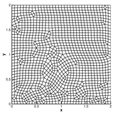
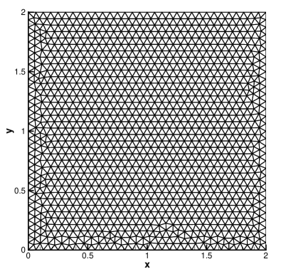
Figure 6: Accuracy test: the unstructured quadrilateral and triangular meshes with cell size $h=1/16$.

  mesh $L^{1}$ error Order $L^{2}$ error Order $1/8$ 1.3752E-02 1.5288E-02 $1/16$ 1.4112E-03 3.28 1.5684E-03 3.28 $1/32$ 2.0183E-04 2.80 2.2400E-04 2.80 $1/64$ 2.3544E-05 3.09 2.6098E-05 3.10  

Table 1: Accuracy test: WENO-3rd with linear weights on quadrilateral meshes.

  mesh $L^{1}$ error Order $L^{2}$ error Order $1/8$ 6.0428E-02 6.9740E-02 $1/16$ 1.2965E-02 2.22 1.5577E-02 2.16 $1/32$ 2.2794E-03 2.50 2.7735E-03 2.48 $1/64$ 1.1090E-04 4.36 1.4425E-04 4.26  

Table 2: Accuracy test: WENO-3rd with non-linear weights on quadrilateral meshes.

  mesh $L^{1}$ error Order $L^{2}$ error Order $1/8$ 4.8752E-03 5.4117E-03 $1/16$ 6.4576E-04 2.92 7.1650E-04 2.92 $1/32$ 8.2542E-05 2.97 9.1507E-05 2.97 $1/64$ 1.0308E-05 3.00 1.1427E-05 3.00  

Table 3: Accuracy test: WENO-3rd with linear weights on triangular meshes.

  mesh $L^{1}$ error Order $L^{2}$ error Order $1/8$ 2.0211E-02 2.5819E-02 $1/16$ 4.6260E-03 2.13 5.4557E-03 2.24 $1/32$ 3.4571E-04 3.74 4.6289E-04 3.56 $1/64$ 1.7427E-05 4.31 2.4689E-05 4.23  

Table 4: Accuracy test: WENO-3rd with non-linear weights on triangular meshes.

5.1 Accuracy tests

The two-dimensional advection of density perturbation is used as the accuracy test. The computational domain is $[0,2]\times[0,2]$ and the initial conditions are given as follows

$$\rho_{0}(x,y)= 1+0.2\sin(\pi(x+y)),~{}p_{0}(x,y)=1,$$

$$U_{0}(x,y)=1,~{}V_{0}(x,y)=1.$$

The periodic boundary conditions are imposed at boundaries and the exact solutions are

$$\rho(x,y,t)= 1+0.2\sin(\pi(x+y-t)),~{}p(x,y,t)=1,$$

$$U(x,y,t)=1,~{}V(x,y,t)=1.$$

The accuracy of the third-order WENO-based gas-kinetic scheme on stationary unstructured quadrilateral and triangular meshes are tested, and the meshes with cell size $h=1/16$ are given in Fig.6 as reference. The $L^{1}$ and $L^{2}$ errors and convergence orders for current scheme are presented in Tab.4 and Tab.4 for quadrilateral meshes, and in Tab.4 and Tab.4 for triangular meshes. The expected order of accuracy is achieved for the current scheme.

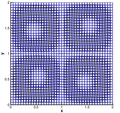
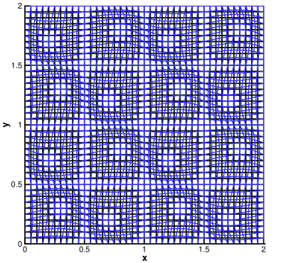
Figure 7: Accuracy test: computational mesh with $40^{2}$ cells at $t=0.5$ for advection of density perturbation for moving-mesh Type-I (left) and Type-II (right).

  mesh $L^{1}$ error Order $L^{2}$ error Order $20^{2}$ 3.2472E-02 1.7989E-02 $40^{2}$ 4.2331E-03 2.93 2.3494E-03 2.93 $80^{2}$ 5.3331E-04 2.98 2.9571E-04 2.99 $160^{2}$ 6.6761E-05 2.99 3.7016E-05 2.99  

Table 5: Accuracy test: 2D advection of density perturbation for moving-mesh Type-I.

  mesh $L^{1}$ error Order $L^{2}$ error Order $20^{2}$ 3.3873E-02 1.8770E-02 $40^{2}$ 4.5521E-03 2.89 2.5410E-03 2.88 $80^{2}$ 5.7874E-04 2.97 3.2386E-04 2.97 $160^{2}$ 7.2641E-05 2.99 4.0674E-05 2.99  

Table 6: Accuracy test: 2D advection of density perturbation for moving-mesh Type-II.

For the accuracy with moving-mesh velocity, two types of time dependent meshes are considered as follows

$$\text{Type-I}:\begin{cases}\displaystyle x(t)=x_{0}+0.05\sin\pi t\sin\pi x_{0}\sin\pi y_{0},\\ \displaystyle y(t)=y_{0}+0.05\sin\pi t\sin\pi x_{0}\sin\pi y_{0}.\end{cases}$$

and

$$\text{Type-II}:\begin{cases}\displaystyle x(t)=x_{0}+0.05\sin\pi t\sin 2\pi x_{0}\sin 2\pi y_{0},\\ \displaystyle y(t)=y_{0}+0.05\sin\pi t\sin 2\pi x_{0}\sin 2\pi y_{0}.\end{cases}$$

where $(x_{0},y_{0})$ is denoted as the initial mesh. The mesh velocity can be directly given during a time step. Initially, $N\times N$ cells are distributed uniformly. The computational meshes with largest deformation at $t=0.5$ are shown in Fig.7 as reference. The $L^{1}$ and $L^{2}$ errors and orders of accuracy at $t=2$ with $N^{2}$ cells are presented in Tab.6 and Tab.6 for two types of moving-mesh with linear weights. The expected accuracy is well kept during the moving-mesh procedure.

  mesh velocity I mesh velocity II mesh $L^{1}$ error $L^{2}$ error $L^{1}$ error $L^{2}$ error $10^{2}$ 4.6940E-15 3.1077E-15 5.2846E-15 3.2855E-15 $20^{2}$ 1.6520E-14 1.1142E-14 1.6967E-14 1.2542E-14 $40^{2}$ 4.2199E-14 2.8577E-14 6.9709E-14 4.3066E-14 $80^{2}$ 1.0889E-13 7.0537E-14 3.2411E-13 2.0728E-13  

Table 7: Accuracy test: geometric conservation law for mesh velocity Type-I and Type-II.

5.2 Geometric conservation law

The geometric conservation law (GCL) [8, 9] is also tested by the time dependent meshes given above. The GCL is mainly about the maintenance of a uniform flow passing through a non-uniform moving mesh. The initial condition for the two-dimensional case is

$$\rho_{0}(x,y)=1,~{}p_{0}(x,y)=1,~{}U_{0}(x,y)=1,~{}V_{0}(x,y)=1.$$

The periodic boundary conditions are adopted as well. The $L^{1}$ and $L^{2}$ errors at $t=0.1$ with $N^{2}$ cells are given in Tab.7 for two types of moving-mesh. The results show that the errors reduce to the machine zero. The geometric conservation law is well preserved by the current scheme.

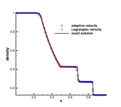
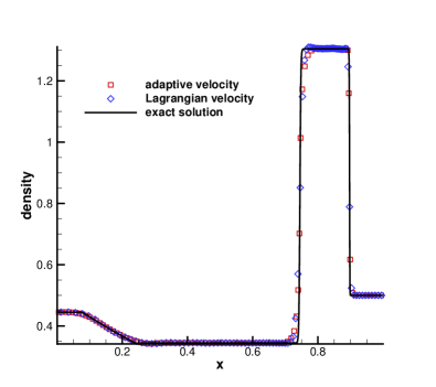
Figure 8: One dimensional Riemann problem: the density distributions for Sod problem at $t=0.2$ (left) and Lax problem at $t=0.16$ (right).

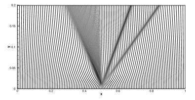
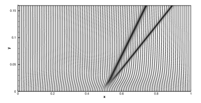
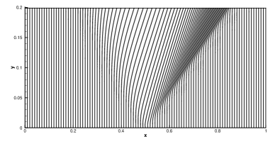
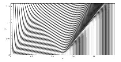
Figure 9: One dimensional Riemann problem: the mesh with adaptation velocity for Sod problem (left) and Lax problem (right).

Figure 10: One dimensional Riemann problem: the mesh with Lagrangian velocity for Sod problem (left) and Lax problem (right).

5.3 One dimensional Riemann problems

In this case, one-dimensional Riemann problems are tested by the current scheme. The first one is the Sod problem, and the initial condition is given as follows

$$(\rho,U,p)=\begin{cases}(1,0,1),&0\leq x<0.5,\\ (0.125,0,0.1),&0.5\leq x\leq 1.\end{cases}$$

The second one is the Lax problem, and the initial condition is given as follows

$$(\rho,U,p)=\begin{cases}(0.445,1.198,3.528),&0\leq x<0.5\\ (0.5,0.5,0.571),&0.5\leq x\leq 1.\end{cases}$$

In the computation, these two cases are tested in the domain $[0,1]\times[0,0.1]$ and non-reflection boundary condition is adopted at the boundaries of computational domain. Initially, $100\times 10$ cells are equally distributed. The adaptation velocity and the Lagrangian velocity are chosen as the mesh velocity. For the adaptive procedure, the parameter $\alpha$ in the monitor function takes $0.1$ for the Sod problem and $0.02$ for the Lax problem. The density distributions for Sod problem at $t=0.2$ and Lax problem at $t=0.16$ with $x=0$ are presented in Fig.8. The history of mesh distribution from adaptation velocity and Lagrangian velocity are presented in Fig.10 and Fig.10. The numerical solutions agrees well with the exact solution. Due the local mesh adaptation, the discontinuities are well resolved by the current scheme.

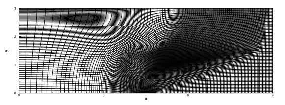
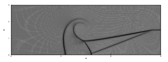
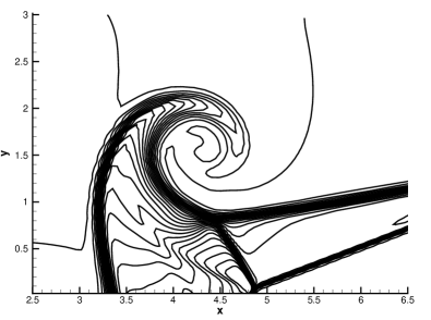
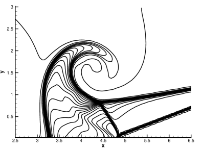
Figure 11: Triple-point problem: the mesh distribution with $180\times 60$ cells with Larangian velocity (top) and adaptation velocity (bottom).

Figure 12: Triple-point problem: the density distribution with Larangian velocity (left) and (right) adaptation velocity with $180\times 60$ cells.

5.3.1 Triple-point problem

The triple-point problem was widely used to validate to the performance of Larangian and ALE methods with large mesh deformation [12, 20]. The initial condition is given as follows

$$(\rho,U,V,p)=\begin{cases}(1,0,0,1),&(x,y)\in D_{1}=[0,1]\times[0,3],\\ (0.125,0,0,0.1),&(x,y)\in D_{2}=[1,9]\times[0,1.5],\\ (1,0,0,0.1),&(x,y)\in D_{3}=[1,9]\times[1.5,3].\end{cases}$$

The non-reflective boundary conditions are used at all boundaries. Left from $x=1$, a high pressure is located in $D_{1}$, which generates a shock wave propagating to the right, and no waves are generated at the beginning at the domain $D_{2}\cup D_{3}$. Initially, $3N\times N$ cells are equally distributed. The adaptation velocity and Lagrangian velocity are chosen as the mesh velocity. For the adaptive procedure, the parameter $\alpha$ in the monitor function takes $0.05$. The mesh distribution with $180\times 60$ cells for Larangian and adaptation velocity at $t=4$ are presented in Fig.12. The density distribution with $180\times 60$ cells for Larangian and adaptation velocity are given in Fig.12, where a vortex appears and swirls the flows around the triple point due to the different shock speeds over the vertical line.

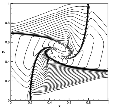
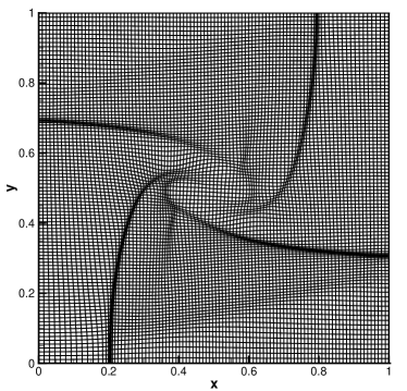
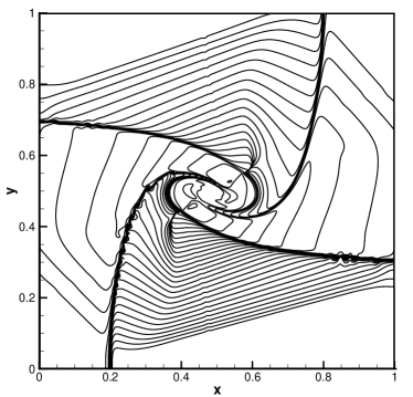
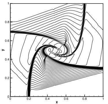
Figure 13: Two dimensional Riemann problem: the density distribution (left) and mesh distribution (right) for four contact discontinuity interaction with $100\times 100$ cells.

Figure 14: Two dimensional Riemann problem: the density distribution on moving-mesh (left) and stationary mesh (right) for four contact discontinuity interaction with $400\times 400$ cells.

5.4 Two-dimensional Riemann problems

In this case, the two-dimensional Riemann problems for Euler equations are presented [22]. The computation domain is $[0,1]\times[0,1]$ and the non-reflection condition is used for the boundaries, and $N\times N$ cells are equally distributed initially. The adaptation velocity are chosen as the mesh velocity. The initial condition is given as follows

$$(\rho,U,V,p) =\left\{\begin{aligned} &(1,0.75,-0.5,1),&x>0.5,y>0.5,\\ &(2,0.75,0.5,1),&x<0.5,y>0.5,\\ &(1,-0.75,0.5,1),&x<0.5,y<0.5,\\ &(3,-0.75,-0.5,1),&x>0.5,y<0.5.\end{aligned}\right.$$

This case is the interaction of planar contact discontinuity for vortex sheets with same signs $J_{12}^{-}J_{32}^{-}J_{41}^{-}J_{34}^{-}$, where $J^{-}_{lr}$ represents the negative contact discontinuity connecting the $l$ and $r$ areas

$$J_{lr}^{-}:w_{l}=w_{r},p_{l}=p_{r},w_{l}^{\prime}\geq w_{r}^{\prime},$$

where $w_{l},w_{r}$ are the normal velocity and $w_{l}^{\prime},w_{r}^{\prime}$ are the tangential velocity. The parameter $\alpha$ in the monitor function takes $0.1$. The density distribution and computational mesh with $100\times 100$ cells are given in Fig.14. The density distribution with $400\times 400$ cells is given in Fig.14. The instantaneous interaction of contacts results in a complex wave pattern, and the instability appears due to the local mesh adaptation. As a reference, the numerical results with stationary mesh is given in Fig.14 as well. The nonlinear combination of linear polynomial smears the discontinuities.

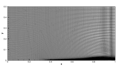
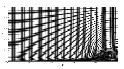
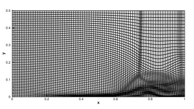
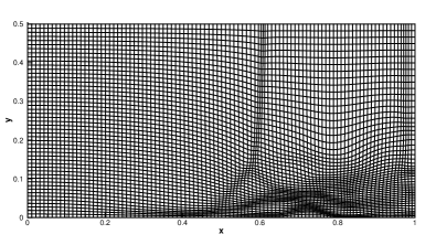
Figure 15: Viscous shock tube: the computational mesh at $t=0.25,0.5,0.75$ and $1$.

5.5 Viscous shock tube

This problem was introduced to test the performances of current scheme for viscous flows [7]. In this case, an ideal gas is at rest in a two-dimensional unit box $[0,1]\times[0,1]$. A membrane located at $x=0.5$ separates two different states of the gas and the dimensionless initial states are

$$(\rho,U,p)=\left\{\begin{aligned} &(120,0,120/\gamma),\ \ \ &0<x<0.5,\\ &(1.2,0,1.2/\gamma),&0.5<x<1,\end{aligned}\right.$$

where $\gamma=1.4$, Reynolds number $\mbox{Re}=200$ and Prandtl number $\mbox{Pr}=0.73$. In the computation, this case is tested in the physical domain $[0,1]\times[0,0.5]$, a symmetric boundary condition is used on the top boundary $x\in[0,1],y=0.5$. Non-slip boundary condition for velocity, and adiabatic condition for temperature are imposed at solid wall boundaries. The membrane is removed at time zero and wave interaction occurs. A boundary layer is generated at the beginning, and a shock moves to the right followed by a contact discontinuity. After reflected by the end wall, the discontinuities interact with the boundary layer.

  Scheme AUSMPW+ [19] M-AUSMPW+ [19] WENO-GKS GKS-ALE Height 0.163 0.168 0.171 0.164  

Table 8: Viscous shock tube: comparison of primary vortex heights among different schemes.

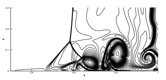
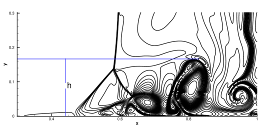
Figure 16: Viscous shock tube: the density distributions on the mesh with $500\times 250$ and $700\times 350$ cells.

To well resolve the complicated two-dimensional shock/shear/boundary-layer interactions, an anisotropy mesh needs to be generated during this procedure. Deferent monitor functions for $x$ and $y$ coordinates takes

$$\omega_{x}=\sqrt{1+0.0001|\partial_{x}(\log\rho)|^{2}},$$

and

$$\omega_{y}=\sqrt{1+0.01|\partial_{y}(\log\rho)|^{2}+0.01|\partial_{y}\sqrt{U^{2}+V^{2}}|}.$$

The computational mesh with $100\times 50$ cells at $t=0.25,0.5,0.75$ and $1$ are given in Fig.15 to present the adaptation procedure. The density distributions on the mesh with $500\times 250$ and $700\times 350$ cells are presented in Fig.16 as well. As shown in Tab.8, the height of primary vortex predicted by the current scheme agrees well with the reference data [19]. However, due to the nonlinear combination of linear polynomial, the current scheme is more dissipative than the fifth-order WENO reconstruction on structured meshes. Currently, the development of higher-order WENO on unstructured meshes is in progress.

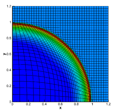
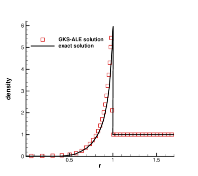
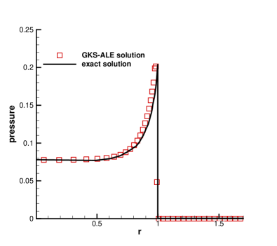
Figure 17: Sedov problem: the mesh and density distribution at $t=1$ with $40\times 40$ cells.

Figure 18: Sedov problem: the density and pressure distribution along the diagonal line $t=1$.

5.6 Sedov blast wave problem

This is a two-dimensional explosion problem to model blast wave from an energy deposited singular point, which is a standard benchmark problem for the Lagrangian method. The fluid is modeled by the ideal gas EOS with $\gamma=1.4$. The initial density has a uniform unit distribution, and the pressure is $10^{-6}$ everywhere, except in the cell containing the origin. For this cell containing the origin, the pressure is defined as $p=(\gamma-1)\varepsilon_{0}/V$, where $\varepsilon_{0}=0.244816$ is the total amount of released energy and $V$ is the cell volume. The reflection condition is used for the left and bottom boundaries, and non-reflection condition is used for the right and top boundaries. The computation domain is $[0,1.2]\times[0,1.2]$ and $40\times 40$ cells are equally distributed initially. The density distribution at $t=1$ is given in Fig.18. The solution consists of a diverging infinite strength shock wave whose front is located at radius $r=1$ at $t=1$ [18]. The density and pressure profile along the diagonal line $t=1$ are given in Fig.18, and the numerical results agrees well with the exact solutions.

5.7 Saltzman problem

This is another benchmark test case for Lagrangian and ALE codes, which tests the ability to capture the shock propagation with a systematically distorted mesh. The computational domain is $[0,1]\times[0,0.1]$. The initial mesh is given by

$$x_{ij} =i\Delta x+(10-j)\Delta y\sin(\frac{i\pi}{100}),$$

$$y_{ij} =j\Delta y,$$

where $\Delta x=\Delta y=0.01$, and $i=0,...,100,j=0,...,10$. An ideal monatomic gas with $\rho=1,e=10^{-4},\gamma=5/3$ is filled in the box. The left-hand side wall acts as a piston with a constant velocity $U_{p}=1$, and other boundaries are reflective walls. As a consequence, a strong shock wave is generated from the left end. At time $t=0.6$, the shock is expected to be located at $x=0.8$, and the post shock solutions are $p=4$ and $p=1.333$. The meshes distribution at $t=0$ and $0.6$ are given in Fig.20. The density and pressure distribution in all the cells at $t=0.6$ is given in Fig.20. The numerical results agrees well with the exact solutions.

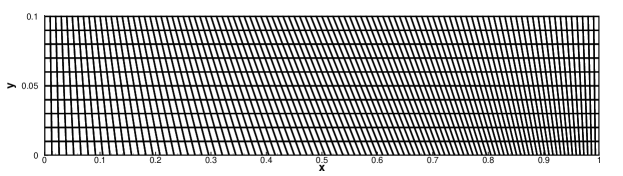
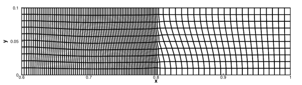
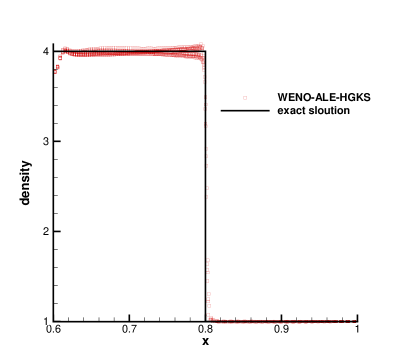
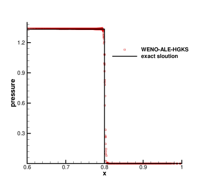
Figure 19: Saltzman problem: the mesh distribution at $t=0$ and $0.6$.

Figure 20: Saltzman problem: the density and pressure distribution in all the cells at $t=0.6$.

6 Conclusion

In this paper, a gas-kinetic scheme is developed based on the third-order WENO reconstruction on unstructured quadrilateral meshes, in which the optimization approach for linear weights and the non-linear weights with new smooth indicator are proposed to improve the robustness of reconstruction. With the arbitrary Lagrangian-Eulerian (ALE) formulation, a high-order moving-mesh gas-kinetic scheme is presented for the inviscid and viscous flows. It extends the third-order gas kinetic method from a static domain to the flow simulation over a variable domain. The two-stage fourth-order method is used for the temporal discretization, and the second-order gas-kinetic solver is used for the flux calculation. In the two-stage method, the spatial reconstruction is performed at the initial and intermediate stage, while the mesh at corresponding stage is given through a specified mesh velocity. To take the mesh velocity along each cell interface into account, the WENO reconstruction is performed at each Gaussian quadrature point in the local moving coordinate. Therefore, the geometric conservation law can be satisfied accurately, which is also verified numerically even with the largely deforming mesh. Numerical examples are presented to validate the performance of current scheme, where the mesh adaptation method and cell centered Lagrangian method can be used to provide mesh velocity.

References

- [1] A.J. Barlow, P.H. Maire, W.J. Rider, R.N. Rieben, M.J. Shashkov, Arbitrary Lagrangian.Eulerian methods for modeling high-speed compressible multimaterial flows J. Comput. Phys. 322 (2016) 603-665.
- [2] D.J. Benson, Computational methods in Lagrangian and Eulerian hydrocodes, Comput. Methods Appl. Mech. Eng. 99 (1992) 235 C394.
- [3] P.L. Bhatnagar, E.P. Gross, M. Krook, A Model for Collision Processes in Gases I: Small Amplitude Processes in Charged and Neutral One-Component Systems, Phys. Rev. 94 (1954) 511-525.
- [4] M. Ben-Artzi, J. Falcovitz, A second-order Godunov-type scheme for compressible uid dynamics, J. Comput. Phys. 55 (1984) 1-32.
- [5] M. Ben-Artzi, J. Li, Hyperbolic conservation laws: Riemann invariants and the generalized Riemann problem, Numerische Mathematik. 106 (2007) 369-425.
- [6] S. Chapman, T.G. Cowling, The Mathematical theory of Non-Uniform Gases, third edition, Cambridge University Press, (1990).
- [7] V. Daru, C. Tenaud, Numerical simulation of the viscous shock tube problem by using a high resolution monotonicity-preserving scheme, Computers Fluids. 38 (2009) 664-676.
- [8] X.G. Deng, M.L. Mao, G.H. Tu, H.Y. Liu, H.X. Zhang, Geometric conservation law and application to high-order finite difference schemes with stationary grids, J. Comput. Phys. 230 (2011) 1100-1115.
- [9] X.G. Deng, Y.B. Min, M.L. Mao, H.Y. Liu, G.H. Tu, H.X. Zhang, Further study on geometric conservation law and application to high-order finite difference schemes with stationary grids, J. Comput. Phys. 239 (2013) 90-111.
- [10] Z.F. Du, J.Q. Li, A Hermite WENO reconstruction for fourth order temporal accurate schemes based on the GRP solver for hyperbolic conservation laws, J. Comput. Phys. 355 (2018) 385-396.
- [11] V. Dyadechko, M.J. Shashkov, Reconstruction of multi-material interfaces from moment data, J. Comput. Phys. 11 (2008) 5361-5384.
- [12] S. Galera, P. H. Maire, J. Breil, A two-dimensional unstructured cell-centered multi-material ALE scheme using VOF interface reconstruction, J. Comput. Phys. 229 (2010) 5755-5787.
- [13] W.H. Hui, P.Y. Li, Z.W. Li, A unified coordinated system for solving the two-dimensional Euler equations, J. Comput. Phys. 153 (1999) 596-637.
- [14] C. Hu, C. W. Shu, Weighted essentially non-oscillatory schemes on triangular meshes, J. Comput. Phys. 150 (1999) 97-127.
- [15] C.W. Hirt, A.A. Armsden, J.L. Cook, An arbitrary Lagrangian Eulerian computing method for all flow speed, J. Comput. Phys. 135 (1997) 203-216.
- [16] C.Q. Jin, K. Xu, A unified moving grid gas-kinetic method in Eulerian space for viscous flow computation, J. Comput. Phys. 222 (2007) 155-175.
- [17] C.Q. Jin, K. Xu, S.Z. Chen, A Three Dimensional Gas-Kinetic Scheme with Moving Mesh for Low-Speed Viscous Flow Computations, Adv. Appl. Math. Mech. 2 (2010) 746-762.
- [18] J.R. Kamm, F.X. Timmes, On efficient generation of numerically robust Sedov solutions, Technical Report LA-UR-07-2849, Los Alamos National Laboratory, 2007.
- [19] K.H. Kim, C. Kim, Accurate, efficient and monotonic numerical methods for multi-dimensional compressible flows Part I: Spatial discretization, J. Comput. Phys. 208 (2005) 527-569.
- [20] M. Kucharik, R.V. Garimella, S.P. Schofield, M.J. Shashkov, A comparative study of interface reconstruction methods for multi-material ALE simulations, J. Comput. Phys. 229 (2010) 2432-2452.
- [21] M. Kucharik, M. Shashkov, Conservative multi-material remap for staggered multi-material Arbitrary Lagrangian-Eulerian methods, J. Comput. Phys. 258 (2014) 268-304.
- [22] P.D. Lax, X.D. Liu, Solution of two-dimensional Riemann problems of gas dynamics by positive schemes, SIAM J. Sci. Comput. 19 (1998) 319-340.
- [23] J. Li, Q. Li, K. Xu, Comparison of the generalized Riemann solver and the gas-kinetic scheme for inviscid compressible flow simulations, J. Comput. Phys. 230 (2011) 5080-5099.
- [24] J.Q. Li, Z.F. Du, A two-stage fourth order time-accurate discretization for Lax-Wendroff type flow solvers I. hyperbolic conservation laws, SIAM J. Sci. Computing, 38 (2016) 3046-3069.
- [25] P. H. Maire, R. Abgrall, J. Breil, J. Ovadia, A cell-centered Lagrangian scheme for two-dimensional compressible flow problems, SIAM J. Sci. Comput. 29 (2007) 1781-1824.
- [26] G.X. Ni, S. Jiang, K. Xu, Remapping-free ALE-type kinetic method for flow computations, J. Comput. Phys. 228 (2009) 3154-3171.
- [27] L. Pan, K. Xu, Q.B. Li, J.Q. Li, An efficient and accurate two-stage fourth-order gas-kinetic scheme for the Navier-Stokes equations, J. Comput. Phys. 326 (2016), 197-221.
- [28] L. Pan, J.Q. Li, K. Xu, A few benchmark test cases for higher-order Euler solvers, Numer. Math. Theor. Meth. Appl. 10 (2017) 711-736.
- [29] L. Pan, K. Xu, Two-stage fourth-order gas-kinetic scheme for three-dimensional Euler and Navier-Stokes solutions, Int. J. Comput. Fluid Dynamics, 32 (2018) 395-411.
- [30] M. Pandolfi, D. D Ambrosio, Numerical instabilities in upwind methods: analysis and cures for the carbuncle phenomenon, J. Comput. Phys. 166 (2001) 271-301.
- [31] X.D. Ren, K. Xu, W. Shyy, A multi-dimensional high-order DG-ALE method based on gas-kinetic theory with application to oscillating bodies, J. Comput. Phys. 316(2016)700-720.
- [32] J. Shi, C. Hu, C.W. Shu, A Technique of Treating Negative Weights in WENO Schemes, J. Comput. Phys. 175 (2002) 108-127.
- [33] C.W. Shu, S. Osher, Efficient implementation of essentially nonoscillatory shock-capturing schemes II, J. Comput. Phys. 83 (1989) 32-78.
- [34] H.Z. Tang, T. Tang, Adaptive mesh methods for one-and two-dimensional hyperbolic conservation laws, SIAM J. Numer. Anal. 41 (2003) 487-515.
- [35] V.A. Titarev, E.F. Toro, Finite volume WENO schemes for three-dimensional conservation laws, J. Comput. Phys. 201 (2014) 238-260.
- [36] E.F. Toro, Riemann Solvers and Numerical Methods for Fluid Dynamics, Third Edition, Springer (2009).
- [37] P. Vachal, R.V. Garimella, M.J. Shashkov, Untangling of 2D meshes in ALE simulations, J. Comput. Phys. 196 (2004) 627-644.
- [38] P. Woodward, P. Colella, Numerical simulations of two-dimensional fluid flow with strong shocks, J. Comput. Phys. 54 (1984) 115-173.
- [39] K. Xu, Direct modeling for computational fluid dynamics: construction and application of unfied gas kinetic schemes, World Scientific (2015).
- [40] K. Xu, A gas-kinetic BGK scheme for the Navier-Stokes equations and its connection with artificial dissipation and Godunov method, J. Comput. Phys. 171 (2001) 289-335.
- [41] F.X. Zhao, L. Pan, S.H. Wang, Weighted essentially non-oscillatory scheme on unstructured quadrilateral and triangular meshes for hyperbolic conservation laws, J. Comput. Phys. 374 (2018) 605-624.