Spatial Positioning Token (SPToken) for Smart Mobility

Abstract

We introduce a permissioned distributed ledger technology (DLT) design for crowdsourced smart mobility applications. This architecture is based on a directed acyclic graph architecture (similar to the IOTA tangle) and uses both Proof-of-Work and Proof-of-Position mechanisms to provide protection against spam attacks and malevolent actors. In addition to enabling individuals to retain ownership of their data and to monetize it, the architecture also is suitable for distributed privacy-preserving machine learning algorithms, is lightweight, and can be implemented in simple internet-of-things (IoT) devices. To demonstrate its efficacy, we apply this framework to reinforcement learning settings where a third party is interested in acquiring information from agents. In particular, one may be interested in sampling an unknown vehicular traffic flow in a city, using a DLT-type architecture and without perturbing the density, with the idea of realizing a set of virtual tokens as surrogates of real vehicles to explore geographical areas of interest. These tokens, whose authenticated position determines write access to the ledger, are thus used to emulate the probing actions of commanded (real) vehicles on a given planned route by “jumping” from a passing-by vehicle to another to complete the planned trajectory. Consequently, the environment stays unaffected (i.e., the autonomy of participating vehicles is not influenced by the algorithm), regardless of the number of emitted tokens. The design of such a DLT architecture is presented, and numerical results from large-scale simulations are provided to validate the proposed approach.

I Introduction

Companies such as Facebook, Google, Amazon, Waze and Garmin are just some examples of corporations that have built successful service delivery platforms using personal data to develop recommender systems. While products gleaned from data mining of personal information have without doubt delivered a great societal value, they have also given rise to a number of ethical questions that are causing a fundamental revision on how data is collected and managed [1]. Some of the most pressing ethical issues include:

• preservation of individuals’ privacy (including GDPR compliance);

• the ability for individuals to retain ownership of their own data;

• the ability for consumers and regulatory agencies alike to confirm the origin, veracity, and legal ownership of data;

• protection against misuse of data by malevolent actors.
  

In this context, Distributed Ledger Technology (DLT) has much to offer. For example, it has been shown in a number of specialized papers (e.g., [2, 3]) that the use of technologies such as blockchain has proven beneficial to alleviate, or even eliminate, some of these above data ethics considerations. Consequently, our objective in this paper is to design one such system. We are particularly interested in developing a DLT-based architecture that supports the design and realization of crowdsourced collaborative recommender systems to sustain a range of mobility applications for smart cities. This objective is challenging for a number of reasons. First, from the perspective of the basic distributed ledger design, the system must support high-frequency microtransactions to facilitate the rapid exchange of information required by the multitude of IoT-enabled devices found in cities. Second, as the DLT must support multiple control actions and recommendations in real time, transaction times should be short. Finally, the ledger architecture should penalize malevolent actors who attempt to spam the system or lie to attack the design of any recommender system based on the DLT.

It is also worth noting that wrapping a DLT layer around personal information will fundamentally change the business model of many companies [4]. Big-data corporations currently monetize recorded personal data with no explicit reward returned to the owner of such data (other than personalized recommendations or free access to products in return for the collected data). In a scenario in which such data is no longer available free-of-charge to these corporations, they would need to find alternative solutions to maintain their quality of service. As an example, imagine a company such as Waze that monitors traffic patterns in cities, and which can build a complete picture of the city environment in almost real time via a telematics platform [5]. If in the future all data became privately held and not available in a public manner, the view of the city environment to this company would be highly uncertain. This disruption will only be alleviated by purchasing data from many car owners. This scenario raises a fundamental question: how to sample privately held data given some desired level of accuracy (e.g., a minimum quality of service)? Given this background, an essential requirement is to develop a set of tools that enable large-scale data sets to be sampled, with a specific objective in mind. For instance, in the Waze example, we wish to reconstruct traffic densities, but obtaining data to build specific predictive tools may require a much more refined data collection procedure. We also wish for the sampling to be done in a manner that allows the veracity of the data to be verified, which enables data owners to be compensated in proportion to the quality of the data they provide.

An additional challenge arises from the design of recommender systems itself. In many important applications, the development of complex decision making tools is inhibited by difficulties in interpreting large-scale, aggregated data sets. This difficulty stems from the fact that data sets often represent closed-loop situations, where actions taken under the influence of decision support tools (i.e., recommenders), or even due to probing of the environment as a part of the model building, do affect the surroundings and consequently the model structure itself. Recently, a number of papers have appeared highlighting the problem of recommender design in closed loop [6, 7, 8, 9, 10]. Even in cases when there is a separation between the effect of a recommender and its environment, the problem of recommender design is complex in many real-world settings due to the challenge of sampling and obtaining real-time data at low cost.

In this paper, we bring both of the above problems together in one framework. In particular, we consider the problem of sampling an unknown density representing traffic flow in a city, comprised of secured data points, using a DLT architecture, without perturbing the density through probing actions. Specifically, we will use reinforcement learning (RL) [11] to explore the density in order to build a model of the environment. Classical RL is usually not applicable for this purpose in many smart city applications due to long training time, and due to the disruptive effects of probing. However, we shall demonstrate that the use of a DLT-based structure allows us to probe the surroundings without affecting it and also enables individuals to not only retain ownership of their own data, but to potentially be rewarded for contributing to the RL framework.

Our paper is structured as follows. Related work is presented in Section 2. In Section 3, we present a distributed ledger design that can be used in smart mobility applications. We then, in Section 4, illustrate how this ledger can be used to facilitate collaborative reinforcement learning algorithms based on crowdsourced information without giving rise to undesirable closed-loop effects (artificial traffic jams). Finally, simulation results are presented in Section 5, and concluding remarks presented in Section 6.

Note to reader: A short version of this paper was an award winner when presented at the International Conference on Connected Vehicles and Expo (ICCVE) 2019 [12]. The present manuscript extends this basic version significantly in several ways.

• All sections of the present paper are more detailed than [12]. The ICCVE paper is a 6 page manuscript whereas the present manuscript is 14 pages long.

• The adaptive Proof-of-Work mechanism described in Section III-B of the present manuscript is not used in [12].

• In [12], each road link represents a state of a Markov chain. In this work, we merge appropriate road segments into a single state when possible (e.g., there is only one action from a given source link). The advantage of this is a significant reduction in the number of states.

• The new road network used in the experimental section is much larger (3663 merged states as opposed to 473 states) than in [12].

• In this work, we also design the state-action space with the following modifications: (i) each state contains an independent subset of actions, and (ii) the set of actions includes two more actions.

• More extensive and realistic simulation results are presented, and all the experiments are new and much more extensive than those in [12].

II Related work

While our work brings together ideas from many areas, the principal idea presented is the use of a DLT to enable distributed reinforcement learning algorithms that can be applied in crowdsourced environments (while avoiding undesirable closed-loop effects). That being said, the paper is not about crowdsourcing per se, and while we use a routing-based RL example to illustrate our architecture, the paper is also not advocating a particular routing policy.

DLT is a term that describes blockchain and a suite of related technologies. From a high-level perspective, a DLT is nothing more than a ledger held in multiple places, and a mechanism for agreeing on the contents of the ledger—namely the consensus mechanism. Since the debut of blockchain in 2008 [13], the technology has been used primarily as an immutable record keeping tool that enables financial transactions based on peer-to-peer trust [14, 15, 16, 17, 18]. Architectures such as blockchain operate a competitive consensus mechanism enabled via mining (i.e., Proof-of-Work), whereas architectures such as the IOTA Tangle [19] based on other graph structures can facilitate cooperative consensus techniques. In our proposed approach, we use a DLT based on the IOTA Tangle. Our interest in IOTA stems from the fact that its architecture is designed to facilitate high-frequency microtrading. In particular, the architecture places a low computational and energy burden on devices using IOTA, it is highly scalable, there are no transaction fees, and transactions are pseudo-anonymous [20]. In terms of mobility applications, we note that several DLT architectures have already been proposed. Recent examples include [21, 22, 23] and the references therein. To the best of our knowledge, our work is the first using a Directed Acyclic Graph (DAG) structure, namely the IOTA Tangle, to support distributed machine learning (ML) algorithms.

In terms of ML, we borrow heavily from RL, Markov Decision Processes (MDPs), and, in particular, crowdsourced ML. The literature on MDPs and RL algorithms is vast and we simply point the reader to some relevant publications in which some of this work is discussed (see [10, 24, 25]). With specific regard to RL and mobility, some applications are presented in [26, 27, 28, 29, 30]. As in our previous work [31], we exploit the idea of using crowdsourced behavioural experience to augment the training of ML algorithms (see [30] for an example of multi-agent RL and a recent survey for an overview of this area in [32]). We also note that our approach bears similarities to the concept of virtual trip lines introduced in [33] and further developed in [34]. However, as we shall see in the sequel, our proposed design goes beyond traffic monitoring: it involves a token-passing mechanism, it uses a DLT-based architecture, it does not depend on GPS traces and it uses Blockchain-like ideas to enforce data sovereignty and spamming prevention. Note that some of these objectives are somewhat related to the literature on classical crowdsourcing [35, 36], where one of the main goals is to quantify data quality in a crowdsourcing setting. In our situation, the use of DLT is motivated by the advantages that the architecture brings to this domain (crowdsourcing): DLT’s built-in consensus mechanism allows, in fact, to both increase quality of data written to ledger, and to prevent spamming. Furthermore, its distributed nature allows the provenance of data to be recorded so that value can later be returned to data owners as the data is used. Also, even though our DLT design uses techniques different to those described in [35, 37], those later techniques are in fact complementary to those proposed here. Namely, those techniques can also apply in our setting to data that is already written in the ledger. This can be viewed as a supplementary layer to the existing DLT architecture, since mechanisms that make difficult writing malicious data to the ledger are in fact intrinsic to the DLT approach (as we shall discuss in later sections). We note also that, as mentioned in [31], our work also has strong links to adaptive control [38]. The idea of augmenting offline models with adaptation is discussed extensively in the recent multiple-models, switching, and tuning paradigm [39].

It is worth mentioning that we are ultimately interested in the design of recommender systems that account for feedback effects in smart city applications. In [40, 41, 42], different information is sent to different agents in an attempt to mitigate closed-loop effects. An alternative, more formal, approach is presented in [10]. There, the authors attempt the identification of a smart city system from closed-loop data sets. Similar issues have drawn interest from various domains including economics [43], recommender systems [44, 7], physiology [45], and control engineering in the context of Smart Cities [8].

Finally, while we have strongly emphasized that this paper is not concerned with routing per se, we nevertheless present an application in which RL is used to learn optimal routes in a complex environment. Although routing is not our focus, we do note that this is a very rich area of research. For a flavour of existing work see, for example, Chapter 5 of [46] for an overview of the literature with specific regard to special vehicles (connected and electric) and the references therein, and the papers [47, 48, 49]. In principle, the crowdsourced DLT-based architecture can be applied in these situations too.

III A distributed ledger for crowdsourced smart mobility - SPToken

III-A Design objectives

Our aim is to design a DLT-based system for crowdsourcing in a smart mobility environment. The DLT is nothing more than a ledger used to record data points and their ownership. Competing devices, namely cars, are able to write data to the ledger in a manner that ensures reliable and high-quality data are written to the ledger. Note that the ledger records data points and their sovereignty, among other information, all of which can be encrypted through classical methods, so that the owner maintains control over who is allowed to access it. A third party then, possibly via monetary payments to the respective data owners, accesses the ledger and uses these data points to run a collaborative algorithm. Value is then returned to individual data owners using some techniques (for example, using the ideas based on Shapley Value [50]). More specifically, in the present paper we explore how to apply this framework to an RL setting where a third party is interested in acquiring information from vehicles in order to solve an optimization problem. In doing this, we focus on how the DLT is used to enable crowdsourced information to realize the RL algorithm (rather than on monetary reward for each vehicle). The underlying idea is to use a set of virtual tokens as a proxy to indicate specific geographical points of interest, whose absolute/relative states and surrounding conditions (e.g., position, speed, nearby air pollution) are of significance for dedicated algorithms. In RL algorithms, for example, we are interested in maximizing the expected reward (relative to an objective function) for taking a specific route across a city. To make this process clearer, consider the following example. Figure 1 shows an instance of a typical scenario where two road junctions $A$ and $B$ are connected to one another through the road segment $\overrightarrow{AB}$. At time $T_{A}$, a vehicle updates the ledger with some collected information $x^{T_{A}}$ (e.g., air pollution level, travel time) by registering at a given visited intersection ($A$, in this example). Intuitively, this can be depicted as if the vehicle leaves a token $\kappa$ with associated information $x^{T_{A}}$ at junction $A$. Then, a new vehicle passing via junction $A$ and directed to junction $B$ can “collect” token $\kappa$ and, as it passes by junction $B$ at time $T_{B}>T_{A}$, it updates the ledger with new information $x^{T_{B}}$ regarding route link $\overrightarrow{AB}$ and the new position of the token. It is noteworthy that in Figure 1 a vehicle leaves the token when it deviates from the token route. Thus, a new car that passes by junction $B$ whose immediate future trajectory coincides with the token’s route will be able to collect the token and the procedure is repeated for a new road segment.

The concept of using tokens to be deposited at specific locations where measurements are needed perfectly conforms with a DLT-based system. In fact, it is natural to use distributed ledger transactions to update the position of available tokens and register the associated data to the points of interest by using transactions (which can be done, for example, using smart sensors at various junctions linked to digital wallets, as shown in Figure 1). Of course, the design of such a network poses a number of challenges that need to be addressed:

• Privacy: In the DLT, transactions are pseudo-anonymous. This is due to the cryptographic nature of the addressing, which is less revealing than other forms of digital payments that are uniquely associated with an individual [51]. Thus, from a privacy perspective, the use of DLT is desirable in a smart mobility scenario.

• Ownership: Transactions in the DLT can be encrypted by the issuer, thus allowing every agent to maintain ownership of their own data. In the aforementioned setting, the only information required to remain public is the current ownership of the tokens.

• Microtransactions: Due to the amount of vehicles in the city environment, and also due to the need for linking the information to real-time conditions (such as traffic ] or pollution levels), there is the demand for a fast and large data throughput.

• Resilience to Misuse: The system must be resilient to attacks and misuse from malevolent actors. Typical examples include double spending attacks, spamming the system, or writing false information to the ledger. All these instances can be greatly limited by a combined use of a consensus system based on Proof-of-Work (PoW) and Proof-of-Position (PoP), which will be described in the next section.

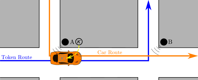
(a) A vehicle passes through a junction $A$ where another car has recently issued some data (this is displayed by a token). This makes the agent eligible to write transactions to the ledger.

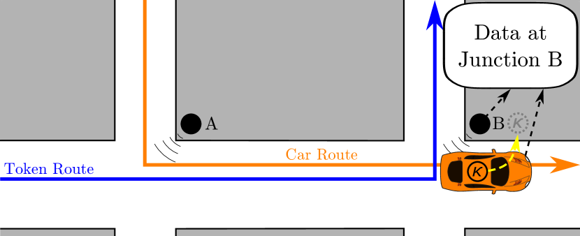
(b) The same vehicle passes through junction $B$. It then writes some data, relative to the road link $\overrightarrow{AB}$, to the ledger and deposits the token so that another vehicle will be able to collect it.

Figure 1: The sequence to issue new data from vehicles. Here $\kappa$ denotes a token. [Clipart from www.clker.com]

To meet all the design objectives described above, in the next section we propose Spatial Positioning Token (SPToken), a permissioned distributed ledger for smart mobility applications, based on the IOTA Tangle.

III-B The Tangle, Proof-of-Position, and Adaptive Proof of Work

As discussed above, we are interested in building a particular Tangle-based, DLT architecture that makes use of DAGs to achieve consensus on the shared ledger. A DAG is a finite connected directed graph with no directed cycles. In other words, in a DAG there is no directed path that connects a vertex with itself. The IOTA Tangle is a particular instance of a DAG-based DLT [20], where each vertex or site represents a transaction, and where the graph with its topology represents the ledger. Whenever a new vertex is added to the Tangle, this must approve a number of previous transactions (normally two). An approval is represented by a new edge added to the graph. Furthermore, in order to prevent malicious users from spamming the network, the approval step requires a small PoW. This step is less computationally intense than its blockchain counterpart [17] and can be easily carried out by common IoT devices, but still introduces some delay for new transactions before they are added to the Tangle. Refer to Figure 2 for a better understanding of this process.

The Tangle architecture has the advantage over blockchain to allow microtransactions without any fees (as miners are not needed to reach consensus over the network [51]), which makes it ideal in an IoT setting as it is described in the previous section. Moreover, the Tangle fits perfectly with the concept of multiple tokens being transferred from one location to another as its DAG structure makes it natural to describe such a process.

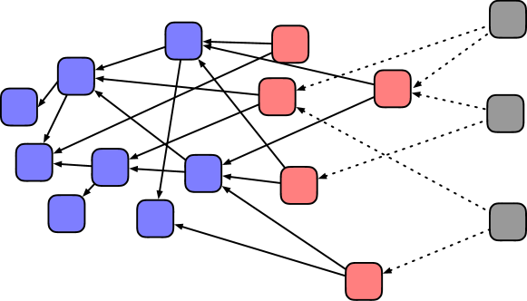
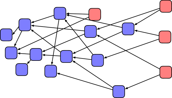
Figure 2: Sequence to issue a new transaction. The blue sites represent the approved transactions and the red ones describe transactions that have not been approved yet. The black edges represent approvals, whereas the dashed ones represent transactions that are performing the PoW in order to approve two unapproved sites.

Unlike the Tangle, in which each user has complete freedom on how to update the ledger with transactions, the SPToken ledger is designed to have an additional regulatory policy in order to prevent agents from adding transactions that do not possess any relevant data (since transactions are encrypted). Therefore, as a further security measure, SPToken makes use of PoP to authenticate transactions: for a transaction to be authenticated, it has to carry proof that the agent was indeed in an area where a token was present, which is achieved via special nodes called observers linked to physical sensors in a city. Whenever a participating car passes by an observer that is in possession of a token, a short range wireless connection is established (e.g., via Bluetooth) and the token is transferred to the vehicle’s account if the requirements are met (e.g., the immediate vehicle’s and token’s future trajectories intersect). To deposit the token and to issue a transaction containing data, the agent needs to pass by another observer and establish a short range connection. See Figure 1 for a better understanding of this process. This process ensures that vehicles have to be physically at the observation points to be able to issue transactions. Such an additional authentication step makes SPToken a permissioned Tangle (similar to permissioned blockchains [14]) i.e. a DAG-based distributed ledger where a certain number of trusted nodes (the observers) are responsible for maintaining the consistency of the ledger (as opposed to a public one, where security is handled by a cooperative consensus mechanism [20]). To keep users from hoarding tokens, the latter should be automatically returned if not used after a certain period of time.

Furthermore, an additional adaptive Proof-of-Work (aPoW) step can be introduced. The aim of this aPoW step is to strategically vary the target difficulty of the PoW to hinder the writing process for “bad” agents that plan to register false information. This is achieved by allowing observers to issue a number of tokens for each desired data point rather than only one. Once each of the vehicles in possession of a token completes a physical PoP step (namely, finishing a road segment), they must also complete a PoW step, the difficulty of which depends on the value of the data they are attempting to write to the ledger. Specifically, vehicles trying to write false data should have to complete a more difficult PoW. The introduction of the aPoW step relies on the assumption that the majority of users will behave honestly and will offer data that is genuine. Moreover, for mobility applications, and thanks to the PoP step, it is reasonable to expect that honest agents taking measurements in the same area, at the same time, will provide similar data (e.g., traffic density, pollution levels).

Consider the event where $N$ users, with writing privileges, each tries to add a data point $x_{i}$ to the DAG, where $x_{i}\in\mathbb{R}^{n},i\in\mathcal{N}$, $\mathcal{N}=\{1,2,\ldots,N\}$. We define $d_{w}(\cdot,\cdot,\cdot)$ to be the amount of work needed to add a new item to the DAG. This work is the difficulty of solving the aPoW step, which is equal to some fixed value $d_{0}$ (representing the minimum amount of work required), plus a term that takes into account the average “distance” between the data $x_{i}$ and all the other items being added at that time. This can be expressed as

$$d_{w}(x_{i},\overline{\text{x}},d_{0})=d_{0}+\alpha\,\left\|x_{i}-\overline{\text{x}}\right\|,$$ (1)

$$\overline{\text{x}}=\dfrac{1}{N}\sum_{j\in\mathcal{N}}x_{j},$$

where $\left\|\cdot\right\|$ is a norm in $\mathbb{R}^{n}$ and $\alpha>0$ is a constant scaling factor. This mechanism ensures that anyone trying to update the ledger with data that are much different from its competitors will have to spend more computing power than other users in order to complete the aPoW. While the aPoW would be straightforward to implement on a regular DLT, its use requires $x_{i}$ and $\overline{\text{x}}$ to be known to all users (in order to check if a nonce that satisfies $d_{w}(x_{i},\overline{\text{x}})$ was found). A possible way to circumvent this problem and maintain the ability to encrypt the data is to operate the following privacy-preserving scheme (for each competitor $i$ in parallel):

1. decompose $x_{i}$ non-uniformly into $N$ fragments $x_{ij}$, such that

   $$\sum_{j\in\mathcal{N}}x_{ij}=x_{i},$$ (2)

   keep $x_{ii}$ and broadcast all the remaining $N-1$ fragments $x_{ij}$, $\forall i\neq j$, to each other competitor $j\in\mathcal{N}-\left\{i\right\}$;

2. receive the corresponding $N-1$ fragments, one from each other competitor, calculate $c_{i}=\sum_{k\in\mathcal{N}}x_{ki}$, and broadcast it to the other competitors;

3. based on the received sum of fragments, compute $\overline{\text{x}}=\dfrac{1}{N}\sum_{k\in\mathcal{N}}c_{k}$;

4. complete $N$ aPoW steps, with difficulty levels $d_{w}\left(x_{ik},\overline{\text{x}}/N,d_{0}/N\right)$, $k\in\mathcal{N}$.

In step 4), for each one of those aPoW steps, competitor $k$ certifies that competitor $i$ has completed its aPoW and that $x_{ik}$ has been issued individually (to avoid cheating). Note that by placing (2) into (1), and since $\left(\cdot\right)$ can be expressed as $\frac{1}{N}\sum_{k\in\mathcal{N}}\left(\cdot\right)$, then we obtain

$$d_{w}(x_{i},\overline{\text{x}},d_{0}) = d_{0}+\alpha\left\|\sum_{k\in\mathcal{N}}x_{ik}-\overline{\text{x}}\right\|$$ (3)

$$= \sum_{k\in\mathcal{N}}\frac{d_{0}}{N}+\alpha\left\|\sum_{k\in\mathcal{N}}\left(x_{ik}-\frac{\overline{\text{x}}}{N}\right)\right\|$$

$$\leq \sum_{k\in\mathcal{N}}\left(\frac{d_{0}}{N}+\alpha\left\|x_{ik}-\dfrac{\overline{\text{x}}}{N}\right\|\right).$$

Using the same notation as in (1), we arrive to

$$d_{w}(x_{i},\overline{\text{x}},d_{0})\leq\sum_{k\in\mathcal{N}}d_{w}\left(x_{ik},\frac{\overline{\text{x}}}{N},\frac{d_{0}}{N}\right),$$ (4)

which means that the proposed privacy-preserving scheme ensures that the overall difficulty of $N$ sequential aPoW steps is at least as large as the difficulty of a single aPoW step. In addition, a further step to make attacks more difficult is to implement a randomized sub-sampled super-majority-based voting system such that spam attacks become easily visible and mitigating measures can be initiated.

Remark: Notice that the idea behind the adaptive PoW, while similar in intent to other consensus mechanisms based on reputation, such as those in [36, 35], also differs from these approaches. In particular, rather than simply labelling a certain data entry as untrustworthy, our approach additionally makes it prohibitively costly for an attacker to write malicious information.

IV Application example - Reinforcement learning over SPToken

In accordance with the design objectives described in Section III, it can be seen that the SPToken architecture is technique-agnostic in the sense that potentially any population-based technique that solves the dynamic routing problem could be used, including not only multi-agent ML but also other methods such as Black-Box Optimization (e.g., evolutionary strategies [52]). However, in order to give a practical illustration of the proposed approach, we will use an RL strategy in combination with the described token-passing architecture. Specifically, instead of using vehicles as RL agents [31] to probe an unknown environment, we use tokens “jumping” among vehicles to effectively create virtual agents and emulate the behaviour of commanded agents designed to probe the surroundings of arbitrary routes. For this, we employ a modified version of the recently proposed RL algorithm called Upper Bounding the Expected Next State Value (UBEV) [53]. UBEV involves a combination of backward induction with maximum likelihood estimation to (i) construct optimistic empirical estimates of state transition probabilities, (ii) assign empirical immediate reward, and (iii) compute optimal policy.

Since long training time is a common disadvantage of RL algorithms, we propose to launch a high number of independent tokens, which act as virtual vehicles and use the same MDP’s policy matrix to explore different areas of a city. In fact, our design of the state-action space allows us to avoid estimating the transition probabilities, which significantly reduces the training time. Effectively, the algorithm learns only the reward distribution which describes the environment (e.g., traffic patterns in a city). We also launch multiple virtual agents that collaborate with each other to speed up the learning process. In addition, introducing tokens enables learning by crowdsourcing without biasing the environment: indeed, if one launched a number of agents, each checking a policy, the corresponding part of the environment could have become congested as a result, and such artificial congestion would be learned by the RL algorithm. SPToken allows one to avoid introducing such biases. Thus, in principle, the token-based technique does not require modification of conventional RL algorithms, and can indeed be applied to any machine learning algorithm. Note also that the concept of tokens does not necessarily require using DLT. However, in our approach we use DLT as a supplementary layer to the RL algorithm in order to facilitate robust data management for real-world deployments. Without the DLT layer, critical aspects such as privacy, authentication, security, robustness to spamming, among others, could be compromised. Our particular DLT implementation, SPToken, manages token collections/deliveries as DLT transactions, and data is validated via the ledger’s consensus algorithms.

Further details of the proposed approach, together with the corresponding experimental assessment, are provided in the following sections. In particular, we experimentally assess:

• how fast the system learns to avoid traffic jams;

• how quickly the system returns to the shortest path policy once the traffic jams clear up;

• how the training time varies with respect to the number of independent tokens.
  

The original UBEV algorithm in [53] performs a standard expectation-maximization trick. Namely, it first fixes the state transition probabilities of the MDP and the expected reward estimates, and uses backward induction to design the optimal deterministic policy which maximizes the expected reward. Next, this policy is used to probe the environment, and the statistics collected over the course of probing are used to update transition probabilities by employing a standard “frequentist” maximum likelihood estimator [54], which simply computes the frequencies of transitioning from one state to another subject to the current action (that can be a function of the current state). Then, the optimal policy (for the updated estimates of the transition probabilities and reward) is recomputed again. This procedure is treated as an episode of the training process and is iterated until convergence (as demonstrated in [53]).

IV-A Modified UBEV algorithm

Recall that an MDP is a discrete-time stochastic control process. Our decision problem is a finite horizon MDP with time horizon $H$, and we assume that the model is known and that the environment is fully observable. An MDP can be represented as a tuple $\langle\mathcal{S},\mathcal{A}_{s},\textbf{P},\mathcal{R}\rangle$, where

• $\mathcal{S}$ is the set of states, with $|\mathcal{S}|=S$ being the number of states;

• $\mathcal{A}_{s}$ is the set of allowable actions, with $|\mathcal{A}_{s}|=A_{s}$ being the number of allowable actions in state $s$, $\mathcal{A}=\bigcup_{s\in\mathcal{S}}\mathcal{A}_{s}$, and with $|\mathcal{A}|=A$ being the total number of actions;

• $\mathrm{P}(s^{\prime}|s,a,t)$ is the probability of transition from state $s$ under action $a\in\mathcal{A}_{s}$ to state $s^{\prime}$ at decision epoch $t\in\mathcal{H}$, $\mathcal{H}=\{1,2,\dots,H\}$;

• $\mathcal{R}(s,a,t)$ is the reward of choosing the action $a\in\mathcal{A}_{s}$ in the state $s$ at decision epoch $t\in\mathcal{H}$.

In an MDP, an agent (i.e., the decision maker) chooses action $a_{t}\in\mathcal{A}_{s}$ at time $t\in\mathcal{H}$ based on observing state $s_{t}$, and then receives a reward $r_{t}$. The trajectory of the MDP is defined as follows: it is assumed that $s_{t+1}\sim\mathrm{P}(\cdot|s_{t},a_{t},t)$, i.e., the state at time $t+1$ is drawn from a distribution P which depends on $s_{t}$, $a_{t}\in\mathcal{A}_{s}$ and decision epoch $t$. In this case, the total expected reward associated to the policy $\pi:\mathcal{S}\to\mathcal{A}$ is defined as

$$\rho(\pi)\coloneqq\mathbb{E}_{s_{1}\dots s_{H}}\left[\sum_{t\in\mathcal{H}}\mathcal{R}(s_{t},\pi(s_{t},t),t)\right]\\ =\sum_{s\in\mathcal{S}}\mathrm{P}_{0}(s)V^{\pi}_{1}(s)\,,$$ (5)

where $\mathrm{P}_{0}$ is the distribution of the initial state, and $V^{\pi}_{t}$ is the value function from decision epoch $t$ for policy $\pi$, formally defined as follows:

$$V_{t}^{\pi}(s)\\ =\mathcal{R}(s,\pi(s,t),t)+\sum_{s^{\prime}\in\mathcal{S}}\mathrm{P}(s^{\prime}|s,\pi(s,t),t)V_{t+1}^{\pi}(s^{\prime}),\\ \quad V_{H+1}^{\pi}\coloneqq 0.$$ (6)

Then, the goal of an agent is to find an optimal trajectory which maximizes the expected reward (5), and the optimal MDP policy (i.e., the policy maximizing Equation (5)) is calculated through the backward induction process given by:

$$\begin{split}\pi(s,t)&=\operatorname*{argmax}_{a\in\mathcal{A}_{s}}\left\{\mathcal{R}(s,a,t)\small{+}\sum_{s^{\prime}\in\mathcal{S}}\mathrm{P}(s^{\prime}|s,a,t)V_{t+1}^{\pi}(s^{\prime})\right\}\\ \pi(s,H)&=\operatorname*{argmax}_{a\in\mathcal{A}_{s}}\mathcal{R}(s,a,H).\end{split}$$ (7)

We are now in a position to present the Modified UBEV (MUBEV) algorithm. Algorithm 1 represents a modified version of the UBEV algorithm as a result of adapting the original UBEV algorithm to our target problem, which includes the following modifications to the UBEV algorithm. First of all, we use a specific state-action space. A state is represented as a collection of road links, while the action space is based on possible directions of connections between the edges of a road network. Namely, we apply the actions 's'—go straight, 'l'—turn left, 'L'—turn partially left, 'R'—turn partially right, 'r'—turn right, and 'u'—stay in the same state (which prevents leaving the destination state). We also exclude U-turns to favor the exploration of the environment, as U-turns may result in undesirable recurrent attempts to use the shortest path policy. The proposed model of the state-action space, based on road links and their interconnections, allows us to provide the algorithm with the set of predefined trivial transition probabilities. For example, let us construct stochastic rows of transition matrices for all possible transitions from state $s_{0}$ assuming that actions 's', 'l', and 'r' are allowable in state $s_{0}$ as shown in Figure 3. This results in

$$\scriptsize{\begin{array}[]{cc}\left[\begin{array}[]{c|>{\centering\arraybackslash$} p{0.1cm} <{$} >{\centering\arraybackslash$} p{0.1cm} <{$} >{\centering\arraybackslash$} p{0.1cm} <{$} >{\centering\arraybackslash$} p{0.1cm} <{$} >{\centering\arraybackslash$} p{0.1cm} <{$} >{\centering\arraybackslash$} p{0.2cm} <{$}}\text{{\bf s}}&s_{0}$\@add@centering&s_{1}$\@add@centering&s_{2}$\@add@centering&s_{3}$\@add@centering&s_{4}$\@add@centering&\cdots$\@add@centering\cr\hline\cr s_{0}&0$\@add@centering&0$\@add@centering&1$\@add@centering&0$\@add@centering&0$\@add@centering&\cdots$\@add@centering\cr\vdots&\vdots$\@add@centering&\vdots$\@add@centering&\vdots$\@add@centering&\vdots$\@add@centering&\vdots$\@add@centering&\ddots$\@add@centering\end{array}\right],&\left[\begin{array}[]{c|>{\centering\arraybackslash$} p{0.1cm} <{$} >{\centering\arraybackslash$} p{0.1cm} <{$} >{\centering\arraybackslash$} p{0.1cm} <{$} >{\centering\arraybackslash$} p{0.1cm} <{$} >{\centering\arraybackslash$} p{0.1cm} <{$} >{\centering\arraybackslash$} p{0.2cm} <{$}}\text{{\bf l}}&s_{0}$\@add@centering&s_{1}$\@add@centering&s_{2}$\@add@centering&s_{3}$\@add@centering&s_{4}$\@add@centering&\cdots$\@add@centering\cr\hline\cr s_{0}&0$\@add@centering&1$\@add@centering&0$\@add@centering&0$\@add@centering&0$\@add@centering&\cdots$\@add@centering\cr\vdots&\vdots$\@add@centering&\vdots$\@add@centering&\vdots$\@add@centering&\vdots$\@add@centering&\vdots$\@add@centering&\ddots$\@add@centering\end{array}\right],\end{array}}$$

$$\scriptsize{\begin{array}[]{cc}\left[\begin{array}[]{c|>{\centering\arraybackslash$} p{0.1cm} <{$} >{\centering\arraybackslash$} p{0.1cm} <{$} >{\centering\arraybackslash$} p{0.1cm} <{$} >{\centering\arraybackslash$} p{0.1cm} <{$} >{\centering\arraybackslash$} p{0.1cm} <{$} >{\centering\arraybackslash$} p{0.2cm} <{$}}\text{{\bf r}}&s_{0}$\@add@centering&s_{1}$\@add@centering&s_{2}$\@add@centering&s_{3}$\@add@centering&s_{4}$\@add@centering&\cdots$\@add@centering\cr\hline\cr s_{0}&0$\@add@centering&0$\@add@centering&0$\@add@centering&0$\@add@centering&1$\@add@centering&\cdots$\@add@centering\cr\vdots&\vdots$\@add@centering&\vdots$\@add@centering&\vdots$\@add@centering&\vdots$\@add@centering&\vdots$\@add@centering&\ddots$\@add@centering\end{array}\right],&\left[\begin{array}[]{c|>{\centering\arraybackslash$} p{0.1cm} <{$} >{\centering\arraybackslash$} p{0.1cm} <{$} >{\centering\arraybackslash$} p{0.1cm} <{$} >{\centering\arraybackslash$} p{0.1cm} <{$} >{\centering\arraybackslash$} p{0.1cm} <{$} >{\centering\arraybackslash$} p{0.2cm} <{$}}\text{{\bf u}}&s_{0}$\@add@centering&s_{1}$\@add@centering&s_{2}$\@add@centering&s_{3}$\@add@centering&s_{4}$\@add@centering&\cdots$\@add@centering\cr\hline\cr s_{0}&1$\@add@centering&0$\@add@centering&0$\@add@centering&0$\@add@centering&0$\@add@centering&\cdots$\@add@centering\cr\vdots&\vdots$\@add@centering&\vdots$\@add@centering&\vdots$\@add@centering&\vdots$\@add@centering&\vdots$\@add@centering&\ddots$\@add@centering\end{array}\right].\end{array}}$$

Clearly, it is not required to learn such trivial transition probabilities, which is a significant advantage especially for large road networks. Note that, in our model, the action 'u' (stay in the same state) is allowable at each state $s\in\mathcal{S}$.

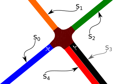
Figure 3: A piece of a road network with five road links representing states $s_{0}$, $s_{1}$, $s_{2}$, $s_{3}$, $s_{4}$. Note that state $s_{3}$ is marked in gray since it is not accessible from state $s_{0}$.

The second modification addresses the following situation. At the beginning of the training, there is a little or no information at all of the reward distribution, and the algorithm rather explores than exploits. By default, the original algorithm always selects the first component of $Q$ (Algorithm 1, line 25) if all the components of the $Q$-function are equal (Algorithm 1, line 22), and thus it probes the environment without any preference in term of the direction of the exploration. In contrast, we force it to stick to the shortest path policy whenever $Q_{i}=Q_{j}$, $\forall i,j$, so that it explores the surrounding along the shortest route. Once the agent faces a traffic jam after a certain action $a\in\mathcal{A}_{s}$, it gets delayed, which in turn introduces the negative reward for the action $a\in\mathcal{A}_{s}$ at state $s$. As a result, the reward distribution changes, and the shortest path policy is amended to avoid the jam by looking for a detour. By operating in this fashion, we sample along near optimal trajectories which has also a practical value.

Algorithm 1 Modified Upper Bounding the Expected Next State Value (UBEV) Algorithm - MUBEV

1:$\mathcal{S}$; $\mathcal{A}$; $H$; P; $\Pi_{SP}$; $M$; $\delta\in\left(0,1\right]$; $r_{max}$.

2:$n(s,a,t)=R(s,a,t)=0;\,\hat{V}(s,t^{\prime})=0;\,\hat{Q}(s,a,t^{\prime})=0$

3:$\forall s,s^{\prime}\in\mathcal{S},\,\,a\in\mathcal{A}_{s},t\in\mathcal{H},\,\,t^{\prime}\in\{1,2,\dots,H+1\}$.

4:$\delta^{\prime}=\delta/9$; $V_{max}=H*r_{max}$.

5:

6:for $k=1,2,3...$ do

7:     // Optimistic planning loop

8:     for $t=H$  to  $1$ do

9:         $\hat{V}_{t+1}=\hat{V}(\cdot,t+1)$

10:         $\tilde{V}_{max}=\min\big{(}\max(\hat{V}_{t+1}),V_{max}\big{)}$

11:         for $s\in\mathcal{S}$ do

12:              for $a\in\mathcal{A}_{s}$ do

13:                  $r=r_{max}$; $EV=\tilde{V}_{max}$

14:                  if $n(s,a,t)>0$ then

15:                       $\eta_{1}=2\ln\ln\left(\max\left(e,n(s,a,t)\right)\right)$

16:                       $\eta_{2}=\ln\left(18*S*A_{s}*H/\delta^{\prime}\right)$

17:                       $\phi=\sqrt{\frac{\eta_{1}+\eta_{2}}{n(s,a,t)}}$

18:                       $\hat{V}_{next}=P(\cdot,s,a,t)\times\hat{V}_{t+1}$

19:                       $EV\small{=}\min\left(\tilde{V}_{max},\hat{V}_{next}+\left(H-t\right)\phi\right)$

20:                       $\hat{r}(s,a,t)=\frac{R(s,a,t)}{n(s,a,t)}$

21:                       $r=\min\left(r_{max},\hat{r}+\phi\right)$                   

22:                  $Q(a)=r+EV$               

23:              $\hat{Q}(s,\cdot,t)=Q$;

24:              if $Q_{i}=Q_{j}\,\,\forall Q_{i},Q_{j}\in Q$ then

25:                  $\tilde{a}=\Pi_{SP}(s,t)$

26:              else

27:                  $\tilde{a}=\operatorname*{argmax}_{a\in\mathcal{A}_{s}}Q(a)$               

28:              $\pi_{k}(s,t)=\tilde{a}$; $\hat{V}(s,t)=Q(\tilde{a})$               

29:     // Execute policy for one episode

30:     $\tilde{s}=\big{[}s_{1}^{(1)},...,s_{1}^{(M)}]\small{\sim}\mathcal{U}\big{(}1,S\big{)},\ s_{1}^{(i)}\small{\neq}s_{1}^{(j)}\ \forall i,j\small{\in}[1,M]$

31:     for $t=1$  to  $H$ do

32:         $a_{t}^{(m)}=\pi_{k}(s_{t}^{(m)},t)$

33:         $s_{t+1}^{(m)}\sim P(\cdot|s_{t}^{(m)},a_{t}^{(m)},t)$

34:         $r_{t}=\mathcal{R}\big{(}s_{t}^{(m)},s_{t+1}^{(m)})$ $\triangleright$ Call to Function 1

35:         $R\big{(}s_{t}^{(m)},a_{t}^{(m)},t^{\prime}\big{)}+=r_{t},\,\,\forall t^{\prime}\in\mathcal{H}$

36:         $n\big{(}s_{t}^{(m)},a_{t}^{(m)},t^{\prime}\big{)}++,\,\,\forall t^{\prime}\in\mathcal{H}$      

Concerning the third modification, we aim to launch multiple tokens always starting at different (randomly sampled) origins and having the same destination. All these tokens follow the same MDP’s policy matrix, and the corresponding collected statistics are then used to update the policy. Therefore, learning and adaptation happen more rapidly.

Finally, we propose a stationary model of the MDP (i.e., transition probabilities and the reward distribution do not vary with time) where each independent agent (token) contributes to the MDP’s reward matrix, and they all use new updated policy in the next episode of the learning process.

Function 1 The Reward Function

1:$s_{t}$; $s_{t+1}$; $\tau(s_{t+1})$; $\alpha$; $\beta$; $w_{D}$; $w_{T}$; $\Omega$; $r_{max}$.

2:$r_{t}$.

3:function $\mathcal{R}$($s_{t}$; $s_{t+1}$)

4:     if $s_{t+1}\neq s_{t}$ then

5:         // Distance reward computation

6:         $d=D(s_{t})-L(s_{t})$

7:         if $d\neq 0$ then

8:              $r_{D}=r_{max}-\frac{D(s_{t+1})}{d}$

9:         else

10:              $r_{D}=r_{max}$          

11:         // Time reward computation

12:         $\tau_{ref}=RY(s_{t+1})+\alpha*\tau_{min}(s_{t+1})$

13:         if $\tau(s_{t+1})\leq\tau_{ref}\ \textbf{or}\ s_{t+1}=s_{f}$ then

14:              $r_{T}=0$

15:         else

16:              $r_{T}=-\beta*\frac{\tau(s_{t+1})}{\tau_{ref}}$

17:             // Applying the edge coefficient

18:              if $RY(s_{t+1})=0$ then

19:                  $r_{T}=r_{T}*EC(s_{t+1})$                        

20:         $r_{t}=w_{D}*r_{D}+w_{T}*r_{T}$ $\triangleright$ Total reward

21:     else$\triangleright$ Jumping to the same state

22:         if $s_{t+1}\neq s_{f}$ then

23:             // Penalty: staying at not destination

24:              $r_{t}=-\Omega$

25:         else

26:              $r_{t}=r_{max}$               return $r_{t}$

Notation for MUBEV and the Reward Function. In Algorithm 1 we have: $\mathcal{S}$ is the set of states; $\mathcal{A}_{s}$ is the set of allowable actions in state $s$, $\mathcal{A}=\bigcup_{s\in\mathcal{S}}\mathcal{A}_{s}$; $S$ and $A$ denote cardinality of finite sets $\mathcal{S}$ and $\mathcal{A}$ respectively; $A_{s}$ denote cardinality of a finite set $\mathcal{A}_{s}$; $H$ is the length of the MDP’s time horizon, with $\mathcal{H}=\{1,2,\cdots,H\}$; P is an array of predefined transition probabilities; $\Pi_{SP}$ is the shortest path policy; $M$ is the number of MUBEV tokens; $\delta$ is the failure probability (see [53] for details); $n(s,a,t)$ is the number of actions $a\in A_{s}$ taken from state $s$ at time $t$; $R(s,a,t)$ is accumulated reward from state $s$ under action $a\in A_{s}$ at time $t$; $\hat{V}(s,t^{\prime})$ is the value function from time step $t^{\prime}$ for state $s$; $\hat{Q}(s,a,t)$ is the Q-function for the appropriate state, action and time [53]. Initial values of elements in arrays $n$, $R$, $\hat{V}$ and $\hat{Q}$ are zeros for all $s\in\mathcal{S},a\in\mathcal{A}_{s},t\in\mathcal{H},t^{\prime}\in\{1,2,\cdots,H+1\}$. Additionally: $r_{max}$ is the maximum reward that the agent can receive per one transition; $V_{max}$ is the maximum value for next states; $\hat{V}(\cdot,t+1)$ and $P(\cdot,s,a,t)$ denote vectors of length $S$, and $\hat{Q}(s,\cdot,t)$ is interpreted as a vector of length $A_{s}$; $\phi$ is the width of the confidence bound [53]; $e$ is the Euler’s number; $\hat{r}(s,a,t)$ is normalized reward from state $s$ under action $a\in A_{s}$ at time $t$; and $r$ and $EV$ are auxiliary variables. Vector $\tilde{s}$ is a vector of initial states of MUBEV tokens, which is uniformly sampled in range from $1$ to $S$ with no repeated entries. The agents (tokens) interact with the environment each time step $t\in\mathcal{H}$, and receive reward $r_{t}$ determined by the reward function defined in Function 1.

Concerning Function 1, it returns total reward, i.e., distance reward plus time reward, at time $t$. Additionally: $\tau(s_{t+1})$ is actual travel time on edges that correspond to state $s_{t+1}$; $\alpha$ is a scale factor that increases minimum travel time on edges due to traffic uncertainties; $\beta$ is a parameter used for faster learning of congestions; $\omega_{D}$ and $\omega_{T}$ are the weights of distance and time reward, respectively; $\Omega$ is the absolute value of penalty given to an agent if it takes action 'u' at a state other than the destination state, or when it leaves the destination; $D(s_{t})$ is the shortest route length from state $s_{t}$ to the destination state $s_{f}$; and $L(s_{t})$ is the length of edges that correspond to state $s_{t}$. Finally, $RY(s_{t+1})$ is the duration of yellow plus red phases of traffic light signals (TLS) that control edges that represent state $s_{t+1}$; if all edges in some state are not controlled by a TLS, we apply $RY=0$ for that state. If some edges are not controlled by traffic light signals, we employ the edge coefficient $EC$ for them (Function 1, lines 13-14) which is computed in this fashion: if the length $L_{t+1}$ of edges that correspond to state $s_{t+1}$ is smaller than the average length $\bar{L}$ of edges included in states, then $EC(s_{t+1})=\left[L(s_{t+1})/\bar{L}\right]^{4}$, otherwise $EC\small=1$.

V Numerical simulations

In the following application, we are interested in designing a recommender system for a community of road users. We distribute a set of MUBEV tokens so that the uncertain environment can be ascertained. These tokens are passed from vehicle to vehicle using the DLT architecture described in Section 3. Specifically, tokens are passed from one vehicle to another in a manner that emulates a real vehicle probing an unknown environment under the instruction of the RL algorithm. The token passing is determined by both the operation of the MUBEV algorithm and the DLT infrastructure, both of which can be orchestrated using a cloud-based service. Vehicles possessing a token are permitted to write data to the DLT. We refer to such vehicles as virtual MUBEV vehicles. In this way, the token passing emulates the behaviour of a real agent (vehicle) that is probing the environment. Once the environment has been learnt, a route recommender system can be built for a community of users interested in route recommendations (e.g., through a smart device app).

For the experimental evaluation of our proposed approach, we designed a number of numerical experiments based on traffic scenarios implemented with the open source traffic simulator SUMO [55]. Interaction with running simulations is achieved using Python scripts and the SUMO packages TraCI and Sumolib. The general setup used in our simulations is as follows:

• In all our experiments, we make use of the area in Dublin, Republic of Ireland shown in Figure 4 (roughly speaking, south Dublin city centre to the canal), with all the U-turns removed from the network file, and a total of $S=3,663$ states.

• A number of roads are selected as origins, destinations, and sources of congestion (see Figure 4). In all experiments we use the set {$O$, $D$} as an origin-destination (OD) pair. We use $C1$ in Experiment 1 and 2 and {$C1$, $C2$} in Experiment 3 to simulate traffic jams on them.

• In all simulations we use a new vehicle type based on the default SUMO vehicle type with maximum speed = 118.8 km/h and impatience = 0.5.

• For the generation of traffic jams, we modify the maximum speed of certain cars to be 6.12 km/h and populate the selected roads with them. When these vehicles are in possession of a token, they become virtual MUBEV vehicles.

• Whenever required, shortest path is obtained via SUMO using the default routing algorithm (dijkstra).

• We refer to the state of an agent as a set of road sections (see Figure 5) and to a token trip as a RL episode.

• We set $H=85$ for the length of the MDP’s time horizon.

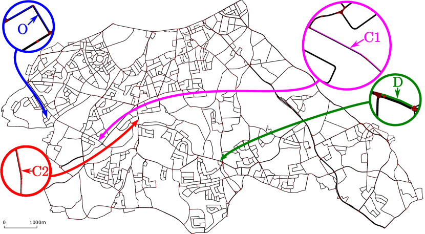
Figure 4: Realistic road network used in the experiments: a part of Dublin, Republic of Ireland. Four road segments of interest are highlighted, namely $O$, $D$, $C1$ and $C2$.

Comment: Note that in our previous works [31, 12], models were developed in which a state corresponded to a single road segment. Such a model is not efficient for number of reasons. First, it leads to prohibitively large RL graphs, even for medium-sized road networks. Second, it also leads to sparse graphs (which can easily be reduced).

To overcome the issues addressed in the above comment, we pre-process the road network to allow the merging of different road links into one state: for a given road link, whenever there is only one incoming direction and only one outgoing direction with neighbor road links, we joint those edges into a single state (as shown in Figure 5). With this preparatory step, the map shown in Figure 4 that contains 10,803 road links results in a graph with only 3,663 states.

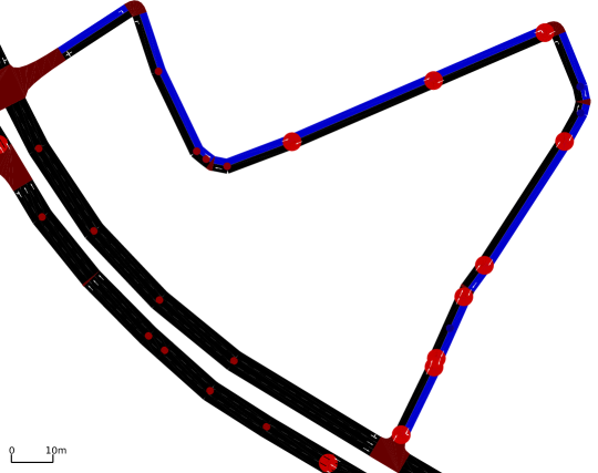
Figure 5: State model: a state corresponds to a set of road links. Road links marked in blue are merged into one state.

Concerning the design parameters of the reward funcion and the MUBEV algorithm, in all our experiments we set $\omega_{D}=\omega_{T}=1$, $r_{max}=1$, $\delta=1$, and tuned the other design parameters as follows: $\alpha=1.2$, $\beta=1.3$, $\Omega=20$. All the experiments rely on a number of background vehicles with random routes which will potentially carry tokens if required. Any specific additional setup for each individual experiment will be described in the corresponding subsection below.

V-A Experiment 1: Optimal route estimation under uncertainty

The purpose of the first experiment is to determine if our DLT-enabled RL approach can estimate a simple unknown environment. To this end, we define the following experiment. We specify an OD pair for which shortest path is known and then, at various time instances, artificially introduce congestion along the shortest path. For this scenario, we aim to show that the token-enabled MUBEV algorithm can distinguish between these two situations, and, in the case of congestion, find the next best route between origin and destination.

Specifically, this first experiment is conducted as follows. We use a single token over each episode of the learning process, meaning that data from the token is used to update the MUBEV policy over every single episode. For this, the MUBEV token has a fixed OD pair given by {$O$, $D$}, and we select the road section labeled as $C1$ in Figure 4 (which belongs to the shortest path for the selected OD pair) to generate a traffic jam on it at different intervals. Then, over each new episode we start the token from $O$ and ask it to travel to $D$, keeping a record of its performance in terms of travel distance (route length) and travel time regardless of its success in attempting to reach $D$. Additionally, the token has a maximum number of allowed links (defined by the length of the MDP’s time horizon) that it can traverse, and if it does not reach its destination within this restriction, then the token trip is declared incomplete (i.e. unsuccessful). The results for this experiment are shown in Figure 6, from which we can draw two main conclusions:

• in general, we can see that the token succeeds in both avoiding traffic jam once congestion is created, and returning to shortest path once congestion is removed, using a reasonably small number of episodes (see Figure 6 bottom);

• as time passes, more statistical information is collected from the environment in the form of reward, and the token is more likely to fully complete a trip for the given OD pair (i.e. red stripes eventually disappear as the experiment progresses in Figure 6).
  

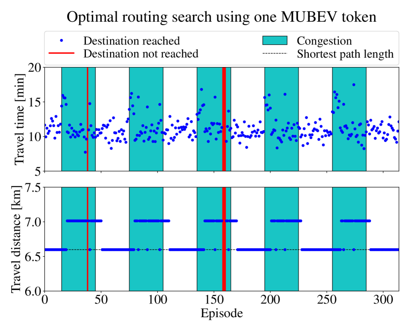
Figure 6: Experiment 1: Travel time and travel distance of a single MUBEV token during the iterative learning process on a changing environment, using a fixed OD pair and approaching an intermittently congested road link ($C1$). Each datapoint corresponds to information registered at the end of each episode (i.e. trip).

These two observations validate our expectations about the UBEV-based routing system: (i) it is able to adapt to uncertain environments, and (ii) its performance improves as time passes. It is worth noting that this experiment is useful to analyze the performance of a single token in the iterative learning process from the environment using a fixed OD pair.

V-B Experiment 2: Optimal route planning under multiple uncertainties

Now we want to evaluate optimal routing under multiple uncertainties. For this, we use a similar setup to that in Experiment 1 (i.e., same OD pair, intermittent traffic jam on $C1$, and one MUBEV token probing the environment), and additionally include a second traffic jam using the following procedure: 1) traffic jam on $C1$ is introduced, 2) the system learns the optimal detour, and 3) second traffic jam is introduced on such an optimal detour (specifically on road link $C2$, as seen in Figure 4). The results of a single realization of this procedure are shown in Figure 7.

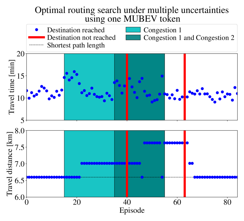
Figure 7: Experiment 2: Travel time and travel distance of a single MUBEV token using a fixed OD pair during the iterative learning process with multiple uncertainties on the environment, namely two intermittently congestions are introduced on $C1$ and $C2$. Each datapoint corresponds to information registered at the end of each episode (i.e. trip).

As it can be seen in Figure 7, a new optimal detour can be learnt after the second traffic jam is created, and the system rapidly returns to the shortest path policy once the two congestions are removed. Recall that red stripes represent uncompleted routes (i.e., the destination state is not reached within an episode), which are more likely to appear once two different congestions are faced.

Note that once the environment has been determined, the resulting route recommendations gleaned from the UBEV-based system can be made available to the wider community of vehicles. We explore this in the following experiment.

V-C Experiment 3: Route recommendations from the UBEV-based system and speedup in learning

The previous experiments are a simple demonstration of the use of MUBEV in a mobility context. We now explore a scenario where multiple tokens, starting from different origins, are used to update the MDP’s policy over each episode. Specifically, in this third experiment, we evaluate the performance of MUBEV as a function of the number of tokens over each episode, subject to a uniform spatial distribution of origins and a common destination (namely, road link $D$). Additionally, we analyze the performance of a test (non-MUBEV) vehicle trying to reach destination $D$ from the given fixed origin $O$, using a recommendation from a simplistic UBEV-based routing system. In this case, the initial recommendation corresponds to the shortest path policy, and further recommendations come from the refinement of such a policy. In addition, if a complete route cannot be calculated using the MUBEV recommender system, then the most recent valid recommendation is reused. Remember that the MDP’s policy is updated at the end of each episode, and thus we only release a new test vehicle at the end of each episode (once the policy has been updated). The results for this experiment, obtained from a total of 250 realizations in order to have a high statistical significance, are depicted in Figures 8, 9 and 10.

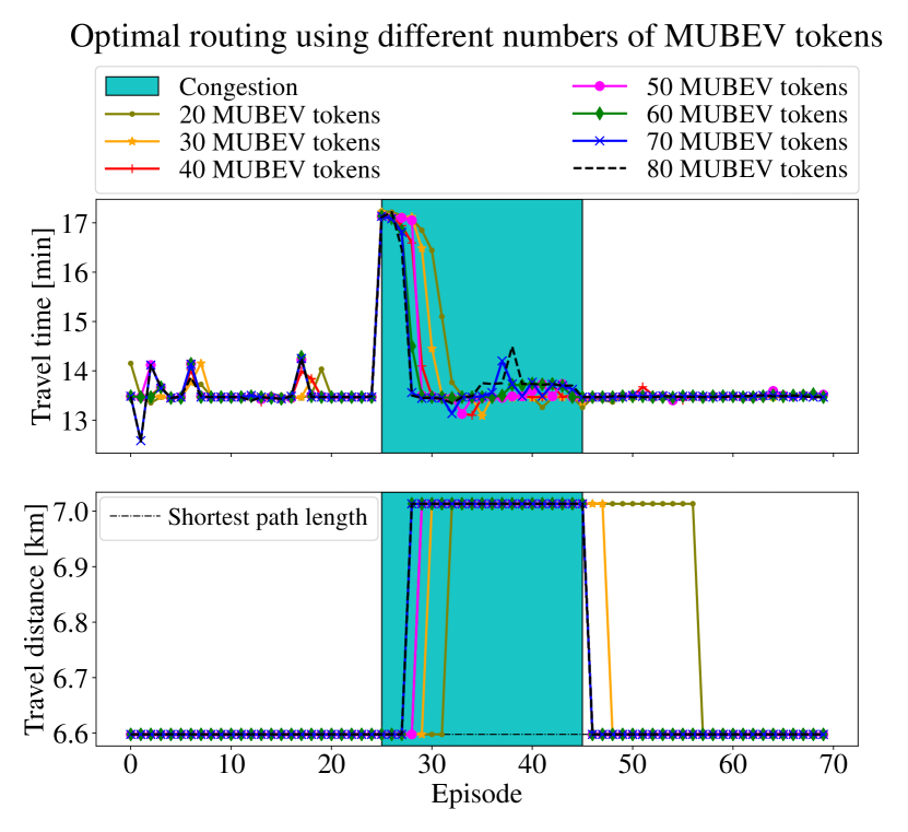
Figure 8: Experiment 3: Median values of travel time/distance of a test vehicle using route recommendations from a UBEV-based routing system involving multiple MUBEV tokens. Each datapoint corresponds to the median value of 250 different realizations of the experiment, with travel time/distance collected at the end of each episode (i.e. trip).

In Figure 8, it can be observed that the number of participating tokens directly affects the convergence rate of the algorithm. As expected, the more tokens involved, the faster the learning process. Figure 9 shows the corresponding 95% median confidence interval (MCI) when using 20, 50 and 80 tokens, respectively, which reflects the high reliability (i.e. narrow MCI range) of our proposed method. From Figure 10, we can notice more conclusively the relationship between the number of MUBEV tokens and the average number of episodes required to learn a new given traffic condition (either congestion or free traffic), which reflects an exponential-like decay.

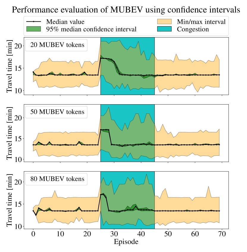
Figure 9: Experiment 3: 95% confidence intervals for the median travel time when using 20, 50 and 80 MUBEV tokens. Each datapoint reflects the analysis per episode of the 250 different realizations of the experiment, with travel time collected at the end of each episode.

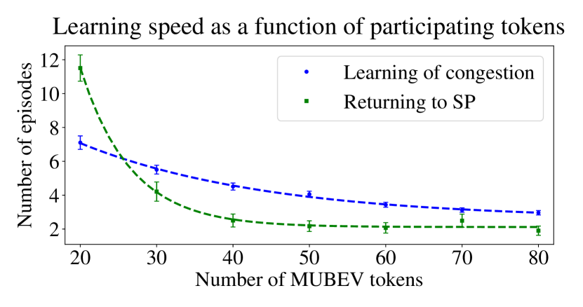
Figure 10: Experiment 3: Average learning speed using multiple MUBEV tokens. Each datapoint corresponds to the average value obtained for 250 different realizations of the experiment. [The error bars represent the 95% confidence interval for the mean. Dashed lines were obtained using exponential curve fitting.]

V-D Experiment 4: SPToken architecture using other optimal policy search algorithm different than MUBEV

The exhaustive list of algorithms for optimal policy search supported by the SPToken architecture does not only include model-based episodic methods (such as UBEV and related) [53, 52], but also model-free episodic methods (such as episodic Q-Learning) [52, 57, 58], and Black-Box Optimization methods (such as Natural Evolution and Neuroevolution strategies) [52, 59]. Since evaluating all the possible alternatives is beyond the scope of this paper, we simply illustrate the generality of our approach by exploring the performance of the system when Q-Learning with Upper-Confidence Bound exploration strategy (UCB Q-Learning) [58] is used instead of MUBEV. The outcome of this is depicted in Figures 11 and 12, obtained from a total of 50 realizations in order to have a reasonable statistical significance for illustration purposes. The results obtained for UCB Q-Learning in the reduced-scale scenario of Experiment 1 (Figure 11) show similarities with respect to Figure 6 (where MUBEV is used): it is clear that the system is able to learn the optimal policy under both free and congested traffic, although UCB Q-Learning falls behind MUBEV in the latter case. The amplified effects of this feature are more evident when analyzing the performance of UCB Q-Learning in the large-scale scenario described in Experiment 3, with Figure 12 displaying exponential-like speedups but with overall improvements less remarkable than the ones obtained with MUBEV. It is worth noting that these performance issues could not only result from the nature of the algorithm employed for the optimal policy search (e.g., whether it is model-free or model-based), but also depend on factors like a comprehensive calibration process, the number of design parameters to be tuned, and the design of a suitable reward function, among others.

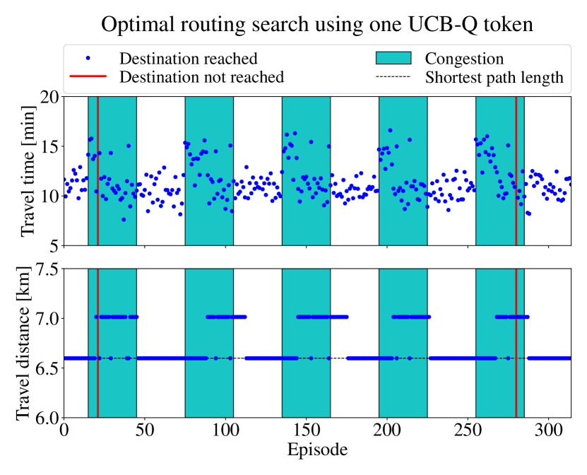
Figure 11: Experiment 4: Travel time and travel distance of a single Q-Learning token, using the setup as in Experiment 1.

Figure 12: Experiment 4: Average learning speed using multiple Q-Learning tokens. Each datapoint corresponds to the average value obtained at the end of 50 different realizations of the experiment. [The error bars represent the 95% confidence interval for the mean. Dashed lines were obtained using exponential curve fitting.]

VI Conclusion and Outlook

We introduced a distributed ledger technology design for smart mobility applications. As a use case of the proposed approach, we presented a DLT-supported distributed RL algorithm to determine an unknown distribution of traffic patterns in a city. Future work will evolve in two directions. We are currently building an SPToken network using our test vehicles at University College Dublin. Our immediate objective is using this framework to test and prototype applications that consume crowdsourced mobility data. A second avenue of research will be theoretical and related to the network delays associated with transactions over a distributed ledger. The impact of such delays on MUBEV and other optimal policy search algorithms are yet to be quantified.

References

- [1] D. Zhang, “Big data security and privacy protection,” in 8th International Conference on Management and Computer Science (ICMCS 2018), Atlantis Press, 2018.
- [2] G. Zyskind, O. Nathan, et al., “Decentralizing privacy: Using blockchain to protect personal data,” in 2015 IEEE Security and Privacy Workshops, pp. 180–184, IEEE, 2015.
- [3] X. Liang, S. Shetty, D. Tosh, C. Kamhoua, K. Kwiat, and L. Njilla, “Provchain: A blockchain-based data provenance architecture in cloud environment with enhanced privacy and availability,” in 2017 17th IEEE/ACM International Symposium on Cluster, Cloud and Grid Computing (CCGRID), pp. 468–477, IEEE, 2017.
- [4] W. Nowiński and M. Kozma, “How can blockchain technology disrupt the existing business models?,” Entrepreneurial Business and Economics Review, vol. 5, no. 3, pp. 173–188, 2017.
- [5] S. v. d. Graaf, “In waze we trust: Algorithmic governance of the public sphere,” Media and Communication, vol. 6, no. 4, pp. 153–162, 2018.
- [6] D. Lazer, R. Kennedy, G. King, and A. Vespignani, “The parable of Google Flu: Traps in big data analysis,” Science, vol. 343, pp. 1203–5, 2014.
- [7] A. Sinha, D. Gleich, and K. Ramani, “Deconvolving feedback loops in recommender systems,” in Proceedings of NIPS, (Barcelona, Spain), 2016. arXiv:1703.01049.
- [8] E. Crisostomi, R. Shorten, and F. Wirth, “Smart cities: A golden age for control theory?,” IEEE Technology and Society Magazine, vol. 35, no. 3, pp. 23–24, 2016.
- [9] L. Bottou, J. Peters, J. Quiñonero Candela, D. X. Charles, D. M. Chickering, E. Portugaly, D. Ray, P. Simard, and E. Snelson, “Counterfactual reasoning and learning systems: The example of computational advertising,” J. Mach. Learn. Res., vol. 14, pp. 3207–3260, Jan. 2013.
- [10] J. P. Epperlein, S. Zhuk, and R. Shorten, “Recovering markov models from closed-loop data,” Automatica, vol. 103, pp. 116 – 125, 2019.
- [11] E. Crisostomi, B. Gaddar, F. Hausler, J. Naoum-Sayawa, G. Russo, and R. Shorten (Editors), Analytics for the sharing economy: Mathematics, Engineering and Business perspectives. Springer.
- [12] R. Overko, R. Ordonez-Hurtado, S. Zhuk, P. Ferraro, A. Cullen, and R. Shorten, “Spatial Positioning Token (SPToken) for Smart Mobility,” 2019. Accepted at The 2019 IEEE ICCVE – International Conference on Connected Vehicles and Expo, ICCVE’19.
- [13] S. Nakamoto, “Bitcoin: A peer-to-peer electronic cash system,” 2008.
- [14] D. Puthal, N. Malik, S. P. Mohanty, E. Kougianos, and G. Das, “Everything you wanted to know about the blockchain: Its promise, components, processes, and problems,” IEEE Consumer Electronics Magazine, vol. 7, no. 4, pp. 6–14, 2018.
- [15] M. Conoscenti, A. Vetro, and J. C. De Martin, “Blockchain for the internet of things: A systematic literature review,” in 2016 IEEE/ACS 13th International Conference of Computer Systems and Applications (AICCSA), pp. 1–6, IEEE, 2016.
- [16] Z. Zheng, S. Xie, H. Dai, X. Chen, and H. Wang, “An overview of blockchain technology: Architecture, consensus, and future trends,” in 2017 IEEE international congress on big data (BigData congress), pp. 557–564, IEEE, 2017.
- [17] M. Banerjee, J. Lee, and K.-K. R. Choo, “A blockchain future for internet of things security: a position paper,” Digital Communications and Networks, vol. 4, no. 3, pp. 149–160, 2018.
- [18] J. Yli-Huumo, D. Ko, S. Choi, S. Park, and K. Smolander, “Where is current research on blockchain technology?—a systematic review,” PloS one, vol. 11, no. 10, p. e0163477, 2016.
- [19] W. Wang, D. T. Hoang, Z. Xiong, D. Niyato, P. Wang, P. Hu, and Y. Wen, “A survey on consensus mechanisms and mining management in blockchain networks,” arXiv preprint arXiv:1805.02707, 2018.
- [20] S. Popov, O. Saa, and P. Finardi, “Equilibria in the tangle,” arXiv preprint arXiv:1712.05385, 2017.
- [21] L. Li, J. Liu, L. Cheng, S. Qiu, W. Wang, X. Zhang, and Z. Zhang, “Creditcoin: A privacy-preserving blockchain-based incentive announcement network for communications of smart vehicles.,” IEEE Trans. Intelligent Transportation Systems, no. 7, pp. 2204–2220.
- [22] Y. Yuan and F.-Y. Wang, “Towards blockchain-based intelligent transportation systems,” in Yuan, Yong, and Fei-Yue Wang. ”Towards blockchain-based intelligent transportation systems.” 2016 IEEE 19th International Conference on Intelligent Transportation Systems (ITSC), pp. 2663–2668, 11 2016.
- [23] A. Dorri, M. Steger, S. S. Kanhere, and R. Jurdak, “Blockchain: A distributed solution to automotive security and privacy.,” CoRR.
- [24] J. Krumm, “A Markov model for driver turn prediction,” tech. rep., SAE Technical Paper, 2008.
- [25] R. Simmons, B. Browning, Y. Zhang, and V. Sadekar, “Learning to predict driver route and destination intent,” in 2006 IEEE Intelligent Transportation Systems Conference, pp. 127–132, Sept. 2006.
- [26] F. Belletti, D. Haziza, G. Gomes, and A. M. Bayen, “Expert level control of ramp metering based on multi-task deep reinforcement learning,” IEEE Transactions on Intelligent Transportation Systems, vol. 19, no. 4, p. 1198–1207, 2017.
- [27] L. Fridman, J. Terwilliger, and B. Jenik, “Deeptraffic: Crowdsourced hyperparameter tuning of deep reinforcement learning systems for multi-agent dense traffic navigation,” arXiv preprint arXiv:1801.02805, 2019.
- [28] P. Mannion, J. Duggan, and E. Howley, “An experimental review of reinforcement learning algorithms for adaptive traffic signal control,” Autonomic Road Transport Support Systems. Springer, pp. 47–66, 2016.
- [29] M. O’Kelly, A. Sinha, H. Namkoong, J. Duchi, and R. Tedrake, “Scalable end-to-end autonomous vehicle testing via rare-event simulation,” arXiv preprint arXiv:1811.00145, 2019.
- [30] S. El-Tantawy, B. Abdulhai, and H. Abdelgawad, “Multiagent reinforcement learning for integrated network of adaptive traffic signal controllers (marlin-atsc): Methodology and large-scale application on downtown toronto,” IEEE Transactions on Intelligent Transportation Systems, vol. 14, no. 3, p. 1140–1150, 2013.
- [31] R. Overko, R. Ordonez-Hurtado, S. Zhuk, and R. Shorten, “Reinforcement Learning Augmented Optimisation for Smart Mobility,” 2019. Accepted at the 58th IEEE Conference on Decision and Control, CDC’19.
- [32] J. W. Vaughan, “Making better use of the crowd: How crowdsourcing can advance machine learning research,” J. Mach. Learn. Res., vol. 18, no. 1, pp. 7026–7071, 2017.
- [33] B. Hoh, M. Gruteser, R. Herring, J. Ban, D. Work, J.-C. Herrera, A. M. Bayen, M. Annavaram, and Q. Jacobson, “Virtual trip lines for distributed privacy-preserving traffic monitoring,” 2008. Proceedings of the 6th international conference on Mobile systems, applications, and services, June 17-20, 2008, Breckenridge, CO, USA.
- [34] B. Hoh, T. Iwuchukwu, Q. Jacobson, D. Work, A. M. Bayen, R. Herring, J. C. Herrera, M. Gruteser, M. Annavaram, and J. Ban, “Enhancing privacy and accuracy in probe vehicle-based traffic monitoring via virtual trip lines,” vol. 11, 5 2012.
- [35] M. Pouryazdan, B. Kantarci, T. Soyata, L. Foschini, and H. Song, “Quantifying user reputation scores, data trustworthiness, and user incentives in mobile crowd-sensing,” IEEE Access, vol. 5, pp. 1382–1397, 2017.
- [36] M. Pouryazdan, B. Kantarci, T. Soyata, and H. Song, “Anchor-assisted and vote-based trustworthiness assurance in smart city crowdsensing,” IEEE Access, vol. 4, pp. 529–541, 2016.
- [37] H. Song, R. Srinivasan, T. Sookoor, and S. Jeschke, Smart Cities: Foundations, Principles, and Applications. Wiley Publishing, 1st ed., 2017.
- [38] K. Narendra and A. Annaswamy, Stable Adaptive Systems. Prentice-Hall, 1988.
- [39] Z. Han and K. Narendra, “New concepts in adaptive control using multiple models,” IEEE Trans. Automat. Contr., vol. 57, pp. 78–89, 01 2012.
- [40] F. Hausler, E. Crisostomi, A. Schlote, I. Radusch, and R. Shorten, “Stochastic park-and-charge balancing for fully electric and plug-in hybrid vehicles,” IEEE Transactions on Intelligent Transportation Systems, vol. 15, pp. 895–901, 2014.
- [41] A. Schlote, B. Chen, and R. Shorten, “On closed-loop bicycle availability prediction,” IEEE Transactions on Intelligent Transportation Systems, vol. 15, pp. 1499–1455, 2015.
- [42] A. Schlote, C. King, E. Crisostomi, and R. Shorten, “Delay-tolerant stochastic algorithms for parking space assignment,” IEEE Transactions on Intelligent Transportation Systems, vol. 15, pp. 1922–1935, 2014.
- [43] H. R. Varian, “Causal inference in economics and marketing,” Proc. of the National Academy of Sciences of the United States of America, p. 7310–7315, 2016.
- [44] D. Cosley, S. K. Lam, I. Albert, J. A. Konstan, and J. Riedl, “Is seeing believing?: How recommender system interfaces affect users’ opinions,” in Proceedings of the SIGCHI conference on Human factors in computing systems, pp. 585–592, ACM, 2003.
- [45] I. D. Loram, H. Gollee, M. Lakie, and P. J. Gawthrop, “Human control of an inverted pendulum: Is continuous control necessary? Is intermittent control effective? Is intermittent control physiological?,” The Journal of Physiology, vol. 589, no. 2, pp. 307–324, 2011.
- [46] E. Crisostomi, R. Shorten, S. Stüdli, and F. Wirth, Electric and Plug-in Hybrid Vehicle Networks: Optimization and Control. Automation and Control Engineering, CRC Press, 2017.
- [47] J. Hu, B. Yang, and C. e. a. Guo, “Risk-aware path selection with time-varying, uncertain travel costs: a time series approach,” The VLDB Journal, vol. 27, 2018.
- [48] B. Yang, J. Dai, and C. e. a. Guo, “Pace: a path-centric paradigm for stochastic path finding,” The VLDB Journal, vol. 27, 2018.
- [49] J. Hu, B. Yang, and C. e. a. Jensen, “Enabling time-dependent uncertain eco-weights for road networks,” Geoinformatica, vol. 17, 2017.
- [50] R. Stanojevic, N. Laoutaris, and P. Rodriguez, “On economic heavy hitters: Shapley value analysis of 95th-percentile pricing,” pp. 75–80, 01 2010.
- [51] P. Ferraro, C. King, and R. Shorten, “IOTA-based Directed Acyclic Graphs without Orphans,” arXiv e-prints, Dec. 2018.
- [52] F. Stulp and O. Sigaud, “Policy improvement methods: Between black-box optimization and episodic reinforcement learning,” 2012.
- [53] C. Dann, T. Lattimore, and E. Brunskill, “Unifying pac and regret: Uniform pac bounds for episodic reinforcement learning,” in Advances in Neural Information Processing Systems, pp. 5713–5723, 2017.
- [54] J. F. T. Hastie, R. Tibshirani, The Elements of Statistical Learning: Data Mining, Inference and Prediction. Springer, 2001.
- [55] P. A. Lopez, M. Behrisch, L. Bieker-Walz, J. Erdmann, Y.-P. Flötteröd, R. Hilbrich, L. Lücken, J. Rummel, P. Wagner, and E. WieBner, “Microscopic traffic simulation using sumo,” in 2018 21st International Conference on Intelligent Transportation Systems (ITSC), pp. 2575–2582, IEEE, 2018.
- [56] J. C. Strelen, “The accuracy of a new confidence interval method,” in Proceedings of the 2004 Winter Simulation Conference, 2004., vol. 1, IEEE, 2004.
- [57] C. Blundell, B. Uria, A. Pritzel, Y. Li, A. Ruderman, J. Z. Leibo, J. Rae, D. Wierstra, and D. Hassabis, “Model-free episodic control,” arXiv preprint arXiv:1606.04460, 2016.
- [58] C. Jin, Z. Allen-Zhu, S. Bubeck, and M. I. Jordan, “Is q-learning provably efficient?,” in Advances in Neural Information Processing Systems, pp. 4863–4873, 2018.
- [59] A. Pritzel, B. Uria, S. Srinivasan, A. P. Badia, O. Vinyals, D. Hassabis, D. Wierstra, and C. Blundell, “Neural episodic control,” in Proceedings of the 34th International Conference on Machine Learning-Volume 70, pp. 2827–2836, JMLR. org, 2017.