Disentangled Attribution Curves for Interpreting Random Forests and Boosted Trees

Abstract

Tree ensembles, such as random forests and AdaBoost, are ubiquitous machine learning models known for achieving strong predictive performance across a wide variety of domains. However, this strong performance comes at the cost of interpretability (i.e. users are unable to understand the relationships a trained random forest has learned and why it is making its predictions). In particular, it is challenging to understand how the contribution of a particular feature, or group of features, varies as their value changes. To address this, we introduce Disentangled Attribution Curves (DAC), a method to provide interpretations of tree ensemble methods in the form of (multivariate) feature importance curves. For a given variable, or group of variables, DAC plots the importance of a variable(s) as their value changes. We validate DAC on real data by showing that the curves can be used to increase the accuracy of logistic regression while maintaining interpretability, by including DAC as an additional feature. In simulation studies, DAC is shown to out-perform competing methods in the recovery of conditional expectations. Finally, through a case-study on the bike-sharing dataset, we demonstrate the use of DAC to uncover novel insights into a dataset.

1 Introduction

Modern machine learning models have demonstrated strong predictive performance across a wide variety of settings. However, these models have become increasingly difficult to interpret, limiting their use in fields such as medicine [1] and policy-making [2]. Moreover, the use of such models has come under increasing scrutiny as they struggle with issues such as fairness [3] and regulatory pressure [4]. To address these concerns, research in interpretable machine learning has received an increasing amount of attention [5, 6]. Interpretable machine learning aims to increase the descriptive accuracy of models (i.e. how well they can be described to a relevant audience) without losing predictive accuracy [5].

Here, we focus on tree ensembles such as random forests [7] and AdaBoost [8], which are widely used and known to have strong predictive performance. However, their complex nonlinear form and sheer number of parameters has made them difficult to interpret, beyond limited notions such as individual feature importance [7, 9, 10].

To address these problems, we introduce Disentangled Attribution Curves (DAC), a method which yields importance curves for any feature (or group of features) to the predictions made by a tree ensemble model. These curves provide a simple post-hoc way to interpret how different features interact within a tree ensemble. Through experiments on real and simulated datasets, we find that DAC provides meaningful interpretations, can identify groundtruth importances, and can be used for simple feature engineering to improve predictive accuracy for a linear model.

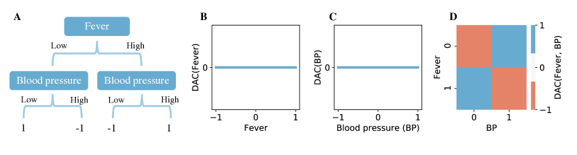
Figure 1: Toy example illustrating DAC. DAC succesfully learns that the interaction between features determines the prediction, not the features in isolation. (A) Tree representing the XOR function. (B, C) DAC single-feature importance for Fever and Blood pressure, respectively. (D) DAC importance for interaction between Fever and Blood pressure.

A simple example

Fig 1 demonstrates a simple example of how DAC works. The tree in Fig 1A depicts a decision tree which performs binary classification using two features (representing the XOR function). In this problem, knowing the value of one of the features without knowledge of the other feature yields no information - the classifier still has a 50% chance of predicting either class. As a result, DAC produces curves which assign 0 importance to either feature on its own (Fig 1B-C). Knowing both features yields perfect information about the classifier, and thus the DAC curve for both features together correctly shows that the interaction of the features produces the model’s predictions.

In this instance, due to their inability to describe interactions, common feature-based importance scores would assign non-zero importance to both features [7, 11, 10]. Consequently, these scalar feature-importance scores are actually an opaque combination of the importance of the individual feature and that feature’s interactions with other features. In contrast, DAC explicitly disentangles the importances of individual features and the interactions between them.

The paper is organized as follows: Sec 2 gives background on related methods, Sec 3 introduces the method, Sec 4 displays results on both simulated and real datasets, and Sec 5 ends with some conclusions.

2 Background

This section briefly covers related work and its relation to DAC.

2.1 Scalar importance scores

The most common interpretations for tree ensembles take the form of scalar feature-importance scores. They are often useful, but their scalar form restricts them from providing as much information as the curves provided by DAC. Importantly, the importance scores for any feature implicitly contain scores for the interaction of that feature with other features, making it unclear how to interpret the feature importance in isolation.

Impurity-based scores (e.g. mean-decrease impurity) [11, 7] are widely used in tree ensemble interpretation. These scores are computed by averaging the impurity reduction for all splits where a feature is used. When using the Gini impurity, these scores are sometimes referred to as the Gini importance.

Another popular score is the permutation importance (i.e. mean decrease accuracy) [7]. It is defined as the mean decrease in classification accuracy after permuting a feature over out-of-bag samples. More recently, this method has been improved to develop conditional variable importance via a conditional permutation scheme [9].

Besides these scores, there are some model-agnostic methods to compute feature importance at the prediction-level (i.e. for one specific prediction) [12]. One popular example is Shap values, which provide prediction-level scores for individual variables [13, 10].

Interaction importance scores

Moving beyond single-variable importance scores, some more recent methods look for interactions between different variables.

For example, recent work [14, 15] stabilizes the training of random forests and then extracts interactions by looking at co-occurrences of features along decision paths. Additionally, some work has begun to address looking at interactions at the prediction-level for random forests (e.g. [10]). Recent methods in the deep learning literature follow a similar intuition of explicitly computing importances for feature interactions [16, 17, 18]. There also exist other methods for calculating interaction importance which are model-agnostic [19, 20].

2.2 Importance curves

Some recent interpretation methods compute curves to convey importances for different features as their value changes. However, these previous methods operate solely on the inputs and outputs of a model, ignoring the rich information contained within the model.

Let $\hat{f}$ be the fitted model of interest, $X$ the input features, $S$ the set of the variables of interest, and $C$ the set of remaining variables. Partial dependence plots (PDP) simply plot the expectation of the marginal function on $X_{S}$ [21], which amounts to integrating out the values of $X_{C}$: $\hat{f}(X_{S})=\mathbb{E}_{X_{C}}\hat{f}(X_{S},X_{C})$. This assumes that the features in $S$ and $C$ are independent, otherwise the points being averaged over do not accurately represent the underlying data distribution. Independence is often an unrealistic assumption which can cause serious issues for this method [9]. Individual conditional expectation (ICE) plots [22] are very similar to PDP (but yield one curve for each data point), and suffer from the same independence assumption.

Aggregated local effects (ALE) plots calculate local differences in predictions based on the variable of interest, conditioned on $x_{C}$ [23]. Then these local effects are aggregated from some baseline. These local effects ameliorate the issue with assuming independent variables, but introduce sensitive hyperparameters, such as a window size and a baseline, which can alter the interpretation. DAC helps fix the need for choosing these hyperparameters by leveraging the internals of the random forest.

3 Disentangled Attribution Curves

DAC yields post-hoc interpretations for tree ensembles which have already been trained. At a high level, DAC importance(s) for a feature (or a group of features) correspond to a fitted model’s average prediction for training data points classified using only that feature (or group of features). This procedure ensures that the importances for individual features and their interactions are disentangled, since the DAC importance for individual features completely ignores other features.

DAC also satisfies the so-called missingness property [13]: features which are not used in the forest do not contribute to the importance for any predictions. This is trivially satisfied, as only features which are used by the forest can change the DAC importance.

Intuitively, DAC is similar to a fairly natural interpretation: the conditional expectation of the model’s predictions over the dataset conditioned on particular values of a feature. However, DAC is superior to the simple conditional expectation curve, as it is more faithful to the model’s underlying process. For example, consider a model which places high importance on only one of two correlated features. Conditional expectation will assign both features a high importance, whereas DAC will successfully learn to assign high importance to only the appropriate feature.

In this paper, we focus on cases where $S$ contains either one or two variables, yielding importance curves or heatmaps, due to the difficulties associated with visualizing more than 3 variables. However, DAC importances can still be used to investigate higher-order interactions between variables.

DAC curves are constructed in a hierarchical fashion, mirroring the structure of a tree ensemble model. In particular, a tree ensemble is a combination of trees, and each tree is a combination of leaves. Given a trained random forest or AdaBoost model, we first define DAC for individual leaves, then demonstrate how to aggregate from leaves to trees, and trees to forests.

3.1 Attribution on leaves

At each leaf node $L$ on a tree $T$, a decision tree makes its prediction by computing the average output value $Y_{i}$ over a subset $R_{L}$ of the input data. Without loss of generality, assume this subset is computed by applying a sequence of decision rules of the form $X_{p}\geq c$. Formally, for a path of length $N$, this corresponds to the region $R$ defined below, resulting in estimate $\hat{Y}$.

$$R_{L} =\bigcap_{j=1}^{N}\{X_{p_{j}}\geq c_{j}\}$$ (1)

$$\hat{Y} =\frac{1}{|R_{L}|}\sum_{i:X_{i}\in R_{L}}Y_{i}$$ (2)

Note that, to compute the region $R_{L}$ requires using information about the set of variables $\{X_{p_{j}}\}_{j=1}^{N}$. To compute our DAC estimate for a set of variables $S$, we restrict $R_{L}$ to $R_{L,S}$ by only using splits for variables which are contained in $S$. In addition, we restrict our consideration to data points $X$ which are close to the center of the leaf. In particular, we require that $|x_{j}-\mu_{L,j}|\leq k\sigma_{L,j}$, for all $j\in S$, where $k$ is a smoothing hyperparameter fixed to one throughout this paper, and $\mu_{L,j},\sigma_{L,j}$ denote the mean and standard deviation of $X_{j}$ contained in $R_{L}$ (if $|R_{L}|=1$, we set $\sigma_{L,j}=0$). This yields our DAC estimate $\hat{Y}_{DAC}(S;L,T)$ for a single leaf:

$$C_{L} =\{x\quad|\quad|x_{j}-\mu_{L,j}|\leq k\sigma_{L,j}\ \forall j\in S\}$$ (3)

$$R_{S,L} =\left(\bigcap_{j=1,p_{j}\in S}^{N}\{X_{p_{j}}\geq c_{j}\}\right)\cap C_{L}$$ (4)

$$\hat{Y}_{DAC}(S;L,T) =\frac{1}{|R_{S,L}|}\sum_{i:X_{i}\in R_{S,L}}Y_{i}$$ (5)

As $\hat{Y}_{DAC}(S;L,T)$ is computed using only splits involving variables contained in $S$, we interpret it as the importance of those variables for making the prediction at this particular leaf.

3.2 Aggregating leaf attributions to trees and forests

Given the estimates $\hat{Y}_{DAC}(S;L,T)$ for the contribution of a set of variables $S$ to the prediction made at an individual leaf $L$ on tree $T$, we now describe how to aggregate those contributions in order to produce an importance curve for a decision tree. When computing the DAC contribution for a particular point $x\in\mathbb{R}^{|S|}$, we take an average over the DAC contributions of leaves $L$ which are “nearby” to $x$. To define proximity, we use the same regions $C_{L}$ as with leaves. Given these regions, we formally define the $DAC$ importance for a given tree at $x$ to be the weighted average of regions $C_{L}$ containing $x$. We weight the average by the size of the regions $|C_{L}|$ in order to account for the size of the leaves in our calculation, and avoid giving undue influence to smaller leaves.

$$f_{DAC}(x;S,T) =\frac{1}{\sum_{L\text{ in tree},x\in C_{L}}|C_{L}|}\underset{L\text{ in tree},x\in C_{L}}{\sum}|C_{L}|\cdot\hat{Y}_{DAC}(S;L,T)$$ (6)

Finally, given an ensemble of trees $T_{1},...,T_{M}$, with corresponding weights $w_{1},...,w_{M}$, we simply define the attribution curve for the tree ensemble to be the weighted average of the attributions for the individual trees $f_{DAC}(x;S,T_{i})$. Note that this mirrors the prediction process for the model, as the predictions for an ensemble of trees are computed by averaging the predictions of it’s constituent trees. In particular, when the ensemble is a random forest, $w_{i}=\frac{1}{M}$.

$$f_{DAC}(x;S)=\sum_{i=1}^{M}w_{i}f_{DAC}(x;S,T_{i})$$ (7)

3.3 An algorithm for computing DAC curves

Algorithm 1 presents pseudocode for computing the tree-level DAC curves $f_{DAC}(x;S,T)$ introduced in Sec 3.1 and Sec 3.2. A simple analysis of the algorithm shows that its time complexity is $O(n\cdot|S|)$, where $n$ is the number of data points in the training set and $|S|$ is the cardinality of the set of features of interest. For a forest, this complexity grows linearly with the number of trees (although they can be very easily parallelized by computing the curve for trees in parallel). In fact, both for-loops in Algorithm 1 can be fully computed in parallel. Similarly, the space complexity of this algorithm is $O(n\cdot|S|)$.

The above analysis assumes summation over $dac$ and $counts$ (the last lines in the for-loop of Algorithm 1 happen in constant time. In practice, the size of these arrays is determined by a pre-specified grid of $X$ values for which the user would like to calculate DAC importances (used to find the size of $dac$ and $counts$). With extremely large grids (beyond what is reasonable in practice), the complexity of the algorithm would depend linearly on the sizes of the arrays $dac$ and $counts$. The above analysis also assumes that the total time complexity for finding the subset of points in each leaf which obey the rules for that leaf across all leaves is $O(n)$.

Algorithm 1 DAC Importance curve generation for a tree

DAC(a tree $T,X,y$, set of features $S$, smoothing parameter $k$)

initialize importance array $dac$ with zero values

initialize counts array $counts$ with zero values

for each leaf $l$ in $T$ :

    # Find the points in a leaf which use rules in $S$

    Let $R$ be the set of rules encountered on the path from the root to $l$ concerning features in $S$

    Let $X^{\prime}$ be the subset of points in $X$ such that for each point $x$, $x$ complies with all rules in $R$

    Let $y^{\prime}$ contain the corresponding $y$ values

    # Ensure feature values in a leaf are not outliers

    for each feature $i$ in $S$ :

         Compute the mean and standard deviation of $X^{\prime}_{i}$, denoted $\mu_{xi}$, $\sigma_{xi}$

         Remove row $j$ in $X^{\prime}$ and $y^{\prime}$ if $X^{\prime}_{j}\notin\mu_{xi}\pm k*\sigma_{xi}$     

    # Add the contribution of this leaf to the DAC curve

    Define $\mu_{y}$ and $c_{y}$ to be the mean and cardinality of $y^{\prime}$ respectively

    Define interval $int$ centered at $(\mu_{xi},...,\mu_{xj})$ and extending by $\pm(\sigma_{xi},...,\sigma_{xj})$

    $dac=dac+\mu_{y}\cdot c_{y}$ over interval $int$

    $counts=counts+c_{y}$ to over interval $int$

return $c$ / $counts$ (normalize elementwise)

4 Results

We now validate, both quantitatively and qualitatively, our introduced DAC importances. First, Sec 4.1 demonstrates that DAC curves can be used as additional features in a linear model to help close the predictive gap between linear models and random forests. Next, through simulation studies, Sec 4.2 quantifies that DAC curves provide a better approximation to conditional expectation than other approaches. Finally, Sec 4.3 shows a case study on the bike-sharing dataset, revealing insights into the data.

4.1 Automated feature engineering with DAC

We now show that single-feature DAC curves produced by Algorithm 1 can be used as additional features to increase the accuracy of a logistic regression model on real-world datasets. This increase in accuracy indicates that DAC curves are capturing meaningful relationships in the data, which are predictive of the outcome in question.

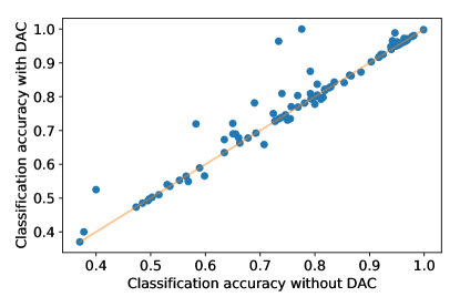
Figure S1: Logistic regression accuracy improves with and without DAC, similiar to Table 1. Each point corresponds to classification accuracy for a different dataset. These datasets are the datasets in PMLB [24] for which a random forest outperforms logistic regression.

To compute these results, we use numerous classification datasets retrieved from the Penn Machine Learning Benchmarks [24]. The datasets include a variety of data types such as classifying liver disorders (the bupa dataset [25]) or evaluating the condition of cars (the car dataset [26]). To find datasets containing significant non-linear effects, we used only datasets where random forests outperformed logistic regression by at least 5% (Fig S1 shows results for datasets where random forests outperform logistic regression by any positive margin).

We randomly partition each of the selected datasets into a training set (75% of the data) and a testing set (25% of the data). We begin by training a random forest model on the training set. Then, the fitted model and the training data are used to identify the feature with the highest Gini importance, and to compute the corresponding single-feature DAC curve.

We then use the computed DAC curve to define a new feature for use by a logistic regression model. The curve is a univariate function which transforms a single feature into its DAC importance. Therefore, for each data point $X$, we append the value of the DAC curve at $X_{i}$, where $i$ is the important feature. On the training set, we fit a logistic regression model using both the original features and the new feature constructed above. Finally, we test the fitted model on the testing set, where we we use the same DAC curve to append the single-feature DAC feature on the testing set .

Table 1 gives results for the accuracy on the testing set. In these instances, adding a single DAC curve feature increased the prediction accuracy, with increases ranging from 3.9% to 23%. The increased accuracy reduces the predictive gap between logistic regression and random forests. In one instance (the bupa dataset), logistic regression with a single DAC curve even outperforms a random forest model (78.2% accuracy versus 75.9% accuracy for the random forest). Classification results for more datasets are given in Fig S1.

While we only append a single 1-dimensional curve here, this process of feature-engineering can be used to append many DAC curves for different features, and even multi-dimensional DAC curves to model interactions between features.

Table 1: Accuracy results on various datasets. Logistic regression trained on data with one DAC curve as an extra feature outperforms logistic regression on the original features.

	monk3	irish	monk1	hayes-roth	bupa	tokyo1	tic-tac-toe	buggyCrx	agaricus-lepiota	car
RF Accuracy	0.971	1.000	0.986	0.825	0.759	0.900	0.950	0.884	1.000	0.977
Logistic Accuracy	0.734	0.776	0.583	0.400	0.690	0.792	0.650	0.740	0.946	0.650
Logistic Accuracy + DAC	0.964	1.000	0.719	0.525	0.782	0.875	0.721	0.809	0.989	0.690
Difference	0.230	0.224	0.137	0.125	0.092	0.083	0.071	0.069	0.042	0.039

4.2 Simulation results

We now use simulations to test how well DAC can recover interactions contained in data. To do so, we generate synthetic data with complex interactions. The functional form of these simulations is in Table 2, based on simulations used in previous work [18].

Table 2: Simulation functions.

$F_{1}({\mathbf{x}})$	$\begin{aligned} &\pi^{x_{1}x_{2}}\sqrt{2x_{3}}-\sin^{-1}(0.5x_{4})+\log(|x_{3}+x_{5}|+1)\end{aligned}$
$F_{2}({\mathbf{x}})$	$\begin{aligned} &\pi^{x_{1}x_{2}}\sqrt{2|x_{3}|}-\sin^{-1}(0.5x_{4})+\log(|x_{3}+x_{5}|+1)-x_{2}x5\end{aligned}$
$F_{3}({\mathbf{x}})$	$\begin{aligned} &\exp|x_{1}-x_{3}|+|x_{2}x_{3}|-x_{3}^{2|x_{4}|}+\log(x_{4}^{2}+x_{5}^{2})\end{aligned}$
$F_{4}({\mathbf{x}})$	$\begin{aligned} &\exp{|x_{1}-x_{3}|}+|x_{2}x_{3}|-x_{3}^{2|x_{4}|}+(x_{1}x_{4})^{2}+\log(x_{4}^{2}+x_{5}^{2})\end{aligned}$
$F_{5}({\mathbf{x}})$	$\begin{aligned} &\frac{1}{1+x_{1}^{2}+x_{2}^{2}+x_{3}^{2}}+\sqrt{\exp(x_{4}+x_{5})}\end{aligned}$
$F_{6}({\mathbf{x}})$	$\begin{aligned} &\exp{(|x_{2}x_{3}|+1)}-\exp(|x_{3}+x_{4}|+1)+\cos(x_{5})\end{aligned}$
$F_{7}({\mathbf{x}})$	$\begin{aligned} &(\arctan(x_{1})+\arctan(x_{2}))^{2}+\max(x_{3}x_{4}+x_{6},0)-\frac{1}{1+(x_{4}x_{5})^{2}}+\sum_{i=1}^{5}{x_{i}}\end{aligned}$
$F_{8}({\mathbf{x}})$	$\begin{aligned} &x_{1}x_{2}+2^{x_{3}+x_{5}}+2^{x_{3}+x_{4}+x_{5}}\end{aligned}$
$F_{9}({\mathbf{x}})$	$\begin{aligned} &\arctan(x_{1}x_{2}+x_{3}x_{4})\sqrt{|x_{5}|}+\exp(x_{5}+x_{1})\end{aligned}$
$F_{10}({\mathbf{x}})$	$\begin{aligned} &\sinh{(x_{1}+x_{2})}+\arccos\left(\arctan(x_{3}+x_{5})\right)+\cos(x_{4}+x_{5})\end{aligned}$

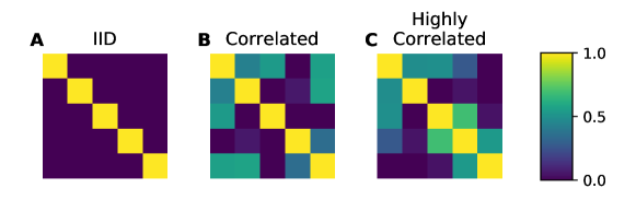
Figure S3: Covariances for different simulation settings in Table 3. Logistic regression accuracy improves with and without DAC, similiar to Table 1. Each point corresponds to classification accuracy for a different dataset. These datasets are the datasets in PMLB [24] for which a random forest outperforms logistic regression by at least five percent.

For each of the functions in Fig 2, we generate a training dataset of 70,000 points and a testing dataset of 15 million points. In all cases, data is generated from a 5-dimensional multivariate Gaussian centered at zero, and points lying outside the interval (-2, 2) are rejected. The data is drawn using different covariance matrices: “IID” refers to the features being independent, “Highly correlated” refers to the features being highly correlated (covariance matrix has eigenvalues 2, 2, 1, 0, 0), and “Correlated” is in between (for specifics, see Fig S3).

We then fit a tree ensemble regressor to the generated training data. From these fitted models, we extract DAC/PDP curves using the training data. Finally, as a proxy for learning the groundtruth interactions, we measure the MSE between these curves and conditional expectation curves calculated on the very large testing set.

Table 3 shows the matches between the DAC and PDP curves with the conditional expectation curves. DAC (the left column) matches the conditional expectation curves better than PDP (the right column) by a substantial margin for different data distributions. This is true even when the features are independent. Comparisons between rows are not meaningful, as they are evaluated with different models and data distributions.

Table 3: Simulation results (averaged over the 5 variables in each of the ten functions in Table 2). Error is standard error of the mean.

	DAC MSE	PDP MSE
RF IID	0.776 $\pm$ 0.110	1.037 $\pm$ 0.147
RF correlated	0.325 $\pm$ 0.052	0.477 $\pm$ 0.076
RF highly correlated	0.553 $\pm$ 0.081	1.459 $\pm$ 0.213
Adaboost IID	1.144 $\pm$ 0.162	13.688 $\pm$ 1.936
Adaboost correlated	1.301 $\pm$ 0.184	21.300 $\pm$ 3.012
Adaboost highly correlated	2.569 $\pm$ 0.115	12.895 $\pm$ 0.577

4.3 Qualitative results

We now use our methods in a case study to show how DAC can provide insights into data. We study the Bike-sharing dataset, a popular dataset in interpretability research [28], made open by the company Capital-Bikeshare with additional features added in a later study [29]. The regression task in the dataset is to predict the hourly count of rented bicycles using a number of features such as the temperature, the time of day, and whether it is a holiday. We fit a random forest to the data and then visualize single-feature and multi-feature DAC curves to understand the interactions it has learned.

Fig 2 shows DAC curves for particular interactions within the data. The heatmaps show 2-dimensional DAC curves (the mean number of rented bicycles in this dataset is 188.7, corresponding to white on the heatmaps). The individual curves on the sides of the heatmaps show 1-dimensional DAC curves for single-feature importance.

Fig 2A shows a qualitatively interesting interaction between the features Hour and Holiday. Within the single-variable context, the Hour feature shows two peaks, corresponding to peak commute times during the day. The curve for Holiday shows that people rent fewer bikes during the holidays (note that this is a binary feature, but we can still evaluate the importance of it at non-binary values based on the forest’s split points). Interestingly, during holidays, the importance of the time of day decreases at peak commuter time, and is now highest in the middle of the day. This makes intuitive sense, as holidays specifically remove commuter traffic.

Fig 2B shows the interaction between Temp and Windspeed. The 1-dimensional Temp curve has a very strong importance for the random forest’s predictions, with higher temperatures resulting in higher model predictions. Windspeed has a relatively smaller effect (note the scale difference for the 1-dimensional curves), and a moderate wind results in the highest predictions. The 2-dimensional DAC curve is largely a superposition of these two curves, suggesting little interaction, although at times there are traces of small interactions between wind speed and temperature. Fig S2 shows more DAC curves for strong interactions between features contained in this model.

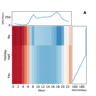
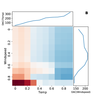
Figure 2: DAC importances and interactions for a random forest fit to the Bike-sharing dataset. Heatmaps show 2-dimensional DAC curves while side plots show 1-dimensional DAC curves.

5 Conclusion

In this paper, we have introduced DAC interpretations for tree ensembles, such as random forests and AdaBoost. For a given feature, or pair of features, DAC produces an importance curve, or heat map, which displays the importance of feature(s) as their value changes. This curve intuitively represents local averages of the model’s predictions based only on the features(s) of interest.

Through an extensive validation, we show that DAC curves can be used as features in a logistic regression model to increase its generalization accuracy. Furthermore, in a simulation study, we show that DAC provides a better approximation to the conditional expectation than competing methods. Finally, through a case study on the bike sharing dataset, we show how DAC can be used to extract insights from real data.

This work opens many potentially promising avenues for future work, such as the use of DAC to automatically extract features (perhaps using higher-order interactions), in order to close the gap between logistic regression and random forests while preserving interpretability. Moreover, we think that ideas used in DAC can be extended to a range of other complex models, such as neural networks. Finally, DAC can be used to automatically explore and identify higher-order interactions then the simple interactions analyzed here, and give further insight into how a tree ensemble is making its predictions.

Supplement

Classification results extended

Qualitative interactions extended

Fig S2A shows the interaction of the features temp with holiday. The peak temperature to rent bikes is decidedly shifted during holidays, indicating that people only bike during very fair weather on their holidays

Fig S2B shows the interaction between Month and Humidity. On its own, month is a feature with a very simple effect that could be equally described by season: people rent fewer bikes during the winter months. Adding humidity broadens the peak month set, and adds more variation to the score on popular and unpopular months. It is clear that people most prefer non-humid summer and fall days to bike, but that biking on a humid hot day is only a slightly better than biking on a humid cold day.

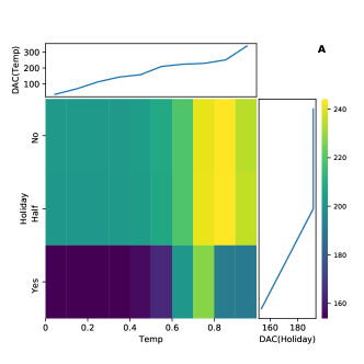
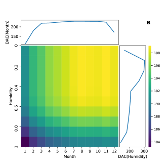
Figure S2: DAC importances and interactions in the Bike dataset.

Simulation settings extended

Finding conditional expectations in real datasets

It is difficult to validate that DAC curves are accurate as there is no groundtruth for what importance should be. As a surrogate, we use the conditional expectation curve calculated on an extremely large data sample.

Specifically, we analyze the regression datasets in PMLB (a disjoint set of datasets as the classification datasets analyzed in Table 1). We fit the model and DAC/PDP curves to 10% of the data. Then, we calculate the conditional expectation curve of the predictions of the model on the other 90% of the data. Table S1 shows the results for the mean squared error between the conditional expectation curve and the DAC/PDP curves. The DAC curve incurs a substantially smaller MSE, suggesting that even with limited data, it is able to estimate the conditional expectations contained in the model.

Table S1: Mean squared error between importance curve (on a small data sample) and conditional expectation curve (on a large data sample). Averaged over multiple features on multiple datasets (9 total points). Error is standard error of the mean.

DAC MSE	PDP MSE
11.843 $\pm$ 3.948	21.175 $\pm$ 7.058

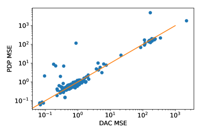
Figure S4: MSE for DAC is generally lower than MSE for PDP. Each point corresponds to MSE for a different dataset (1,521 points total). These datasets are the regression datasets in PMLB [24] for which a random forest outperforms logistic regression by at least five percent. Excluded a few points for which the MSE is above $10^{6}$, as these points are poorly fit by the random forest.

References

- [1] Geert Litjens, Thijs Kooi, Babak Ehteshami Bejnordi, Arnaud Arindra Adiyoso Setio, Francesco Ciompi, Mohsen Ghafoorian, Jeroen AWM van der Laak, Bram van Ginneken, and Clara I Sánchez. A survey on deep learning in medical image analysis. Medical image analysis, 42:60–88, 2017.
- [2] Tim Brennan and William L Oliver. The emergence of machine learning techniques in criminology. Criminology & Public Policy, 12(3):551–562, 2013.
- [3] Cynthia Dwork, Moritz Hardt, Toniann Pitassi, Omer Reingold, and Richard Zemel. Fairness through awareness. In Proceedings of the 3rd innovations in theoretical computer science conference, pages 214–226. ACM, 2012.
- [4] Bryce Goodman and Seth Flaxman. European union regulations on algorithmic decision-making and a" right to explanation". arXiv preprint arXiv:1606.08813, 2016.
- [5] W James Murdoch, Chandan Singh, Karl Kumbier, Reza Abbasi-Asl, and Bin Yu. Interpretable machine learning: definitions, methods, and applications. arXiv preprint arXiv:1901.04592, 2019.
- [6] Finale Doshi-Velez and Been Kim. Towards a rigorous science of interpretable machine learning. arXiv preprint arXiv:1702.08608, 2017.
- [7] Leo Breiman. Random forests. Machine learning, 45(1):5–32, 2001.
- [8] Yoav Freund, Robert E Schapire, et al. Experiments with a new boosting algorithm. In icml, volume 96, pages 148–156. Citeseer, 1996.
- [9] Carolin Strobl, Anne-Laure Boulesteix, Thomas Kneib, Thomas Augustin, and Achim Zeileis. Conditional variable importance for random forests. BMC bioinformatics, 9(1):307, 2008.
- [10] Scott M Lundberg, Gabriel G Erion, and Su-In Lee. Consistent individualized feature attribution for tree ensembles. arXiv preprint arXiv:1802.03888, 2018.
- [11] Leo Breiman, Jerome Friedman, RA Olshen, and Charles J Stone. Classification and regression trees. Chapman and Hall/CRC, 1984.
- [12] Marco Tulio Ribeiro, Sameer Singh, and Carlos Guestrin. Why should i trust you?: Explaining the predictions of any classifier. In Proceedings of the 22nd ACM SIGKDD International Conference on Knowledge Discovery and Data Mining, pages 1135–1144. ACM, 2016.
- [13] Scott M Lundberg and Su-In Lee. A unified approach to interpreting model predictions. In Advances in Neural Information Processing Systems, pages 4768–4777, 2017.
- [14] Sumanta Basu, Karl Kumbier, James B Brown, and Bin Yu. iterative random forests to discover predictive and stable high-order interactions. Proceedings of the National Academy of Sciences, page 201711236, 2018.
- [15] Karl Kumbier, Sumanta Basu, James B Brown, Susan Celniker, and Bin Yu. Refining interaction search through signed iterative random forests. arXiv preprint arXiv:1810.07287, 2018.
- [16] Chandan Singh, W James Murdoch, and Bin Yu. Hierarchical interpretations for neural network predictions. arXiv preprint arXiv:1806.05337, 2018.
- [17] W James Murdoch, Peter J Liu, and Bin Yu. Beyond word importance: Contextual decomposition to extract interactions from lstms. arXiv preprint arXiv:1801.05453, 2018.
- [18] Michael Tsang, Dehua Cheng, and Yan Liu. Detecting statistical interactions from neural network weights. arXiv preprint arXiv:1705.04977, 2017.
- [19] Jerome H Friedman, Bogdan E Popescu, et al. Predictive learning via rule ensembles. The Annals of Applied Statistics, 2(3):916–954, 2008.
- [20] Christoph Molnar, Giuseppe Casalicchio, and Bernd Bischl. Quantifying interpretability of arbitrary machine learning models through functional decomposition. arXiv preprint arXiv:1904.03867, 2019.
- [21] Jerome H Friedman. Greedy function approximation: a gradient boosting machine. Annals of statistics, pages 1189–1232, 2001.
- [22] Alex Goldstein, Adam Kapelner, Justin Bleich, and Emil Pitkin. Peeking inside the black box: Visualizing statistical learning with plots of individual conditional expectation. Journal of Computational and Graphical Statistics, 24(1):44–65, 2015.
- [23] Daniel W Apley. Visualizing the effects of predictor variables in black box supervised learning models. arXiv preprint arXiv:1612.08468, 2016.
- [24] Randal S Olson, William La Cava, Patryk Orzechowski, Ryan J Urbanowicz, and Jason H Moore. Pmlb: a large benchmark suite for machine learning evaluation and comparison. BioData mining, 10(1):36, 2017.
- [25] James McDermott and Richard S Forsyth. Diagnosing a disorder in a classification benchmark. Pattern Recognition Letters, 73:41–43, 2016.
- [26] Marko Bohanec and Vladislav Rajkovic. Knowledge acquisition and explanation for multi-attribute decision making. In 8th Intl Workshop on Expert Systems and their Applications, pages 59–78, 1988.
- [27] Fabian Pedregosa, Gaël Varoquaux, Alexandre Gramfort, Vincent Michel, Bertrand Thirion, Olivier Grisel, Mathieu Blondel, Peter Prettenhofer, Ron Weiss, Vincent Dubourg, et al. Scikit-learn: Machine learning in python. Journal of machine learning research, 12(Oct):2825–2830, 2011.
- [28] Christoph Molnar. Interpretable machine learning. A Guide for Making Black Box Models Explainable, 2018.
- [29] Hadi Fanaee-T and Joao Gama. Event labeling combining ensemble detectors and background knowledge. Progress in Artificial Intelligence, 2(2-3):113–127, 2014.