SCALAR: Simultaneous Calibration of 2D Laser and Robot Kinematic Parameters Using Planarity and Distance Constraints

Abstract

In this paper, we propose SCALAR, a calibration method to simultaneously calibrate the kinematic parameters of a 6-DoF robot and the extrinsic parameters of a 2D Laser Range Finder (LRF) attached to the robot’s flange. The calibration setup requires only a flat plate with two small holes carved on it at a known distance from each other, and a sharp tool-tip attached to the robot’s flange. The calibration is formulated as a nonlinear optimization problem where the laser and the tool-tip are used to provide planar and distance constraints, and the optimization problem is solved using Levenberg-Marquardt algorithm. We demonstrate through experiments that SCALAR can reduce the mean and the maximum tool position error from 0.44 mm to 0.19 mm and from 1.41 mm to 0.50 mm, respectively.

Note to Practitioners— Many industrial robotic applications require the robotic system to be calibrated in order to achieve the demanded accuracy. Unfortunately, existing calibration processes are often cumbersome or require expensive measurement systems. This paper presents a novel calibration method to calibrate simultaneously a 6-DoF industrial robot and a 2D laser scanner attached to the robot’s flange. The method only uses the data from the robot and the laser, so there is no need for external measurement systems. The laser scanner can also be used after the calibration for subsequent robot tasks such as scanning a workpiece to accurately determine its location. The calibration setup only requires a flat plane and a sharp tool-tip attached on the robot’s flange. The proposed method is easy to deploy and is more cost-effective than existing calibration methods.

I Introduction

Traditional robotics applications, such as pick and place, spray-painting and spot-welding, rely on the high repeatability of existing industrial robots and hence tend to overlook accuracy. However, there is an increasing number of applications (e.g. robotic on-demand fulfillment, robotic 3D printing [1], etc.) where the robot must adapt dynamically to a changing environment and hence the robot’s accuracy becomes crucial. Consider for instance the robotic drilling task in [2] where the robot is required to drill several holes at precisely-defined locations on a workpiece. The workpiece can vary for each task, and the placement within the workspace may not be precisely known. To tackle such task automatically the robot has to scan the workspace, determine the location of the workpiece, and finally move to the drilling locations, all of which have to be done accurately. The accuracy of such a system depends on at least two factors: the accuracy of the robot and the accuracy of the measurement system.

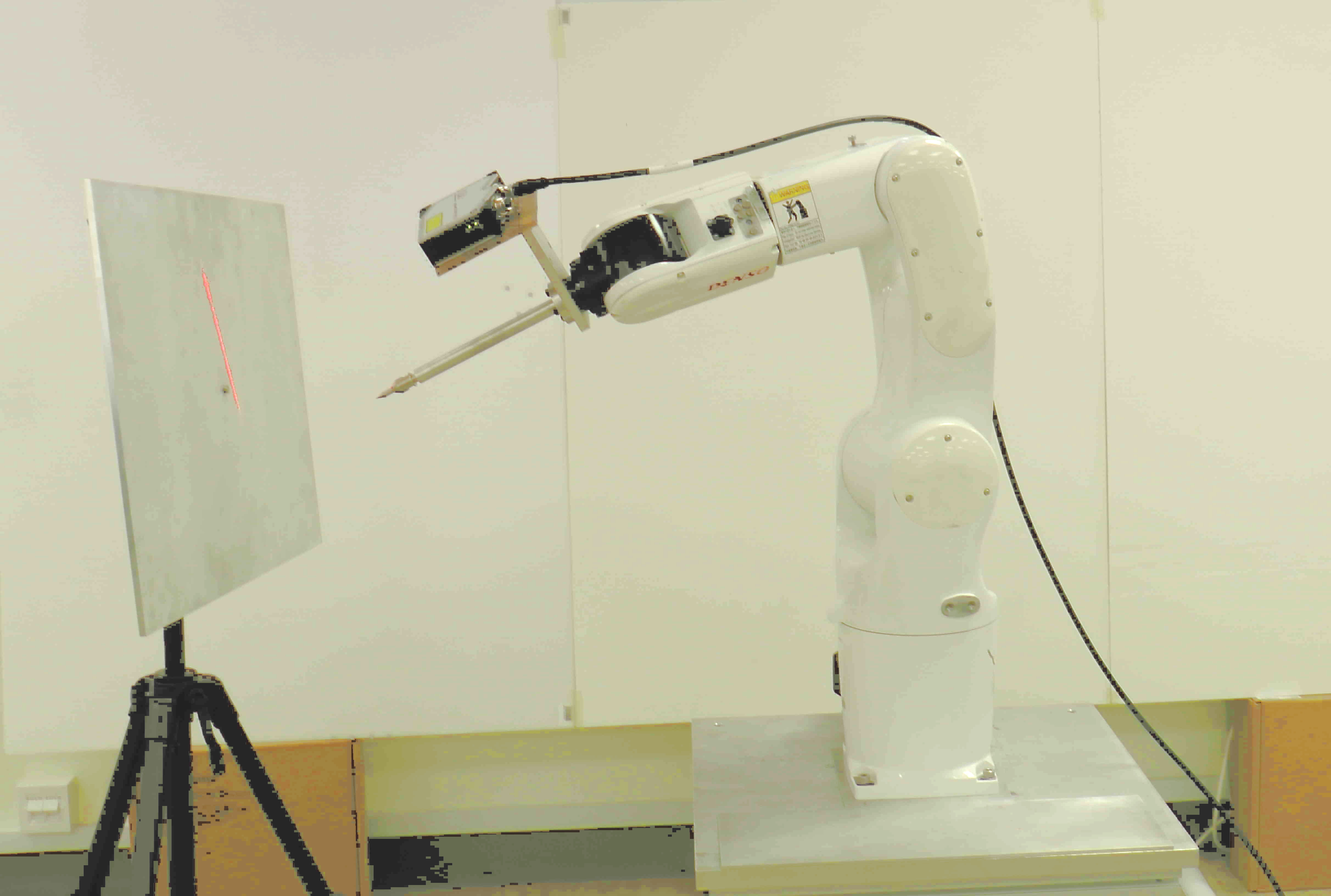
Figure 1: Calibration Setup: A 6-DoF industrial robot equipped with a 2D Laser Range Finder and a sharp tool. A flat plate is located within the robot’s workspace and the LRF’s ray is projected onto the plate.

The accuracy of the robot is determined by how close the robot’s model is to the actual kinematic parameters of the robot. Robot kinematic calibration is usually conducted to achieve a higher accuracy, either by an external measurement system or by constraining the motion of the end-effector.

To improve the accuracy of the measurement system, intrinsic calibration and extrinsic calibration are often necessary. Intrinsic calibration refines the internal parameters of the measurement devices (e.g. focal length and lens distortion for camera), while extrinsic calibration refines the transformation between the measurement system and the robot coordinate system. In addition, the type of the measurement device also affects the accuracy. For example. a near-range laser scanner commonly used in industry for workpiece profiling can achieve a very high accuracy (on the order of $\text{\,}\mathrm{\SIUnitSymbolMicro m}$). For such high-accuracy device, the intrinsic calibration is often performed by the manufacturer, so only the extrinsic calibration is required.

In [3] we proposed an earlier version of SCALAR, which we shall refer to as SCALAR_α in this article, to calibrate simultaneously the kinematic parameters of a 6-DoF robot and the extrinsic parameters of a 2D Laser Range Finder (LRF)using only the information provided by the LRF attached to the robot’s flange. The LRF was chosen because it costs one order of magnitude less than commonly used measurement systems (such as Vicon or FARO Laser Tracker). Moreover, it can be used during the subsequent robotic tasks. For example, the robot can move the LRF to scan the workpiece in the drilling task [2] to determine the holes’ positions accurately .

We reported the performance of SCALAR_α for a simulated system in [3]. During experiments with our real setup we found that since SCALAR_α calibrates simultaneously the robot’s and the laser’s parameters, each system, taken in isolation, is not properly calibrated. That is, neither the robot’s kinematic parameters, nor the laser’s extrinsic parameters converge to the good values, although the combined system is accurate. We did not encounter this errors during simulation but only during the experiments with the real setup. In the experiments there are multiple sources of error that perturb the calibration process and cause it to deviate from the actual values.

In this paper, we present an improvement over SCALAR_α, which will be called SCALAR in this article. The key idea is to introduce an additional distance constraint to the optimization problem, such that the robot’s kinematic parameters converge to good values. This distance constraint is obtained by moving a tooltip attached to the robot’s end-effector through a known distance, and recording the robot’s joint values at the beginning and the end of the movement.

The remainder of the paper is as follows. In Section II we discuss existing approaches for calibrating robot’s kinematic parameters and LRF’s extrinsic parameters. In Section III, SCALAR is explained in detail. The experimental results are presented in Section IV to verify SCALAR, and finally we conclude with a few remarks in Section V.

II Related works

II-A Calibration of robot’s kinematic parameters

Existing robot calibration procedures can be divided in two categories: unconstrained and constrained calibration. In unconstrained calibration, an external measurement system is required to precisely determine the pose of the robot’s end-effector. Some of the examples of unconstrained calibration works include Ye et al. [4], Ginani and Mota [5], Nubiola and Bonev [6], and Wu et al. [7], who use measurement systems such as Faro Laser Tracker, Romer Measurement Arm, and SMX Laser Tracker to calibrate the robot. There are two limitations for this type of calibration methods: the calibration setup is cumbersome and the external measurement systems are very expensive.

As alternative, several researchers have focused on developing calibration methods that rely on the sensors available in the robotic systems combined with poses restricted by pre-engineered constraints, i.e. constrained calibration. The constraints can be in the form of point constraints [8], surface constraints, – in [9] the authors manufactured a cylinder and used its curved surface as constraint – or, planar constraints [10, 11, 12, 13, 14, 15, 16].

In [17], Wang et al. use point constraint in the form of a ball with a known radius, and the robot moves the laser attached to it to measure the center of the ball. In [18] and  [19], Liu et al. obtain the point constraint by using a laser pointer and a Position-Sensitive Detector (PSD), but they only calibrate the joint offset instead of the whole robot kinematic parameters.

Ikits and Hollerbach [12] propose a kinematic calibration method using a planar constraint via a touch probe. While the approach is promising, they also report that some of the parameters are hardly observable when the measurements are noisy or when the model is incomplete. In [13], Zhuang et al. investigate robot calibration with planar constraints, in particular the observability conditions of the robot’s kinematic parameters. They prove that a single-plane constraint is insufficient for calibrating a robot’s kinematics, and a minimum of three planar constraints are necessary.

Joubair and Bonev [16] calibrate both the kinematic and non-kinematic (stiffness) parameters of a FANUC LR Mate 200iC industrial robot using planar constraints in the form of a high precision 9-inches granite cube. The robot is equipped with an MP250 Renishaw touch probe, which is then moved to touch four planes of the granite cube. The granite cube’s face is flat to within $0.002$ mm. In another work [20], Joubair and Bonev use distance and sphere constraints in the form of a triangular plate with three 2-inch spheres separated at known distance.

In [21], Choi et al. calibrate the extrinsic parameters of a multi-camera system and the DH parameters of a pan-tilt unit (regarded as a 2-DoF robot manipulator) simultaneously. One of the camera is attached to the pan-tilt unit, and a fiducial marker is used to provide the reference frame for all the cameras. In their work, however, the focus is more about calibrating the camera system instead of the manipulator, and the manipulator used only has 2-DoF. In [22], the work is extended to a 5-DoF robot manipulator.

II-B Calibration of extrinsic 2D LRF parameters

Extrinsic calibration of an LRF consists of finding the correct homogeneous transformation from the robot coordinate frame to the laser coordinate frame. Most of the works on extrinsic calibration of an LRF involves a camera, since both sensors are often used together. The works in this field are largely based on Zhang and Pless’ work [23]. They propose a method to calibrate both a camera and an LRF using a planar checkerboard pattern. The checkerboard pattern provides the planar constraints for an optimization problem where both camera and laser parameters are optimized simultaneously using Levenberg-Marquardt algorithm. Unnikrishnan and Hebert [24] use the same setup as [23], but they do not optimize the camera parameter simultaneously. Wenyu et al. [25] propose a noise tolerant algorithm using a planar disk with arbitrary orientation to calibrate the laser sensor. Li et al. [26] calibrate a 3D laser sensor using a calibration sphere.

II-C Novelty of the proposed method

SCALAR can be seen as a combination of the algorithm for extrinsic calibration of an LRF [23] and the algorithm for calibration of robot’s kinematic parameters using planar constraints [16]. In [3] we described the advantages of SCALAR over the existing methods: a) The parameters of the robot and of the laser are calibrated simultaneously, b) No expensive external measurement system is required, c) The calibration plate can be easily manufactured, and d) Calibration poses can be distributed globally in the robot’s workspace. Unlike our previous work in SCALAR_α [3], SCALAR uses only two planar constraints and an additional distance constraint, and the resulting robot’s kinematic parameters are more accurate.

III Method

The calibration setup is depicted in Fig. 1, where a flat plate is placed within the reachable robot workspace. There are two small holes on the plate separated by a known distance $D$. An LRF and a sharp tool-tip are attached to the robot flange. The calibration procedure can be divided into four steps:

1. The plate is moved to two ($k=2$) different locations. For each location, the robot is moved to $N$ poses such that the LRF’s ray is directed to the respective plate. One reading from the 2D LRF ray contains hundreds of data points, so $M$ data points are selected randomly for each pose (after removing the outliers by standard line fitting with RANSAC), and the robot’s joint angles are recorded.

2. The plate is moved to $L=15$ additional locations. For each location, the robot is moved such that the tool-tip touches the pair of holes on the plate consecutively without changing the end-effector orientation. The tool-tip orientation may vary between different plate locations, but at any particular location the robot has to maintain the same orientation between the pair of holes.

3. A tool calibration is performed so that the position of the tool-tip with respect to the robot’s flange is known.

4. Finally, the Levenberg-Marquardt nonlinear optimization algorithm is used to calibrate the all the parameters (robot kinematic and LRF extrinsic parameters) based on the collected data.

The calibration algorithm remains largely the same as SCALAR_α [3], except with the addition of the distance constraint and the reduction of the plane locations from three to two locations. Hence, we will focus on the part where SCALAR differs from SCALAR_α.

The calibration algorithm can be described as follows. First, the initial estimate of the LRF’s extrinsic parameters are obtained using the linear least-squares method with the data from one of the plates’s location in Step 1. This is based on the algorithm in [23] and presented in detail in  [3]. Next, the robot kinematic parameters and the LRF’s extrinsic parameters are optimized simultaneously to satisfy the planar and distance constraints using Levenberg-Marquardt nonlinear optimization method. The optimization method requires the tool-tip coordinates w.r.t. the robot’s flange, so the next section describes the tool calibration to obtain the tool-tip coordinates accurately. Finally, we present how Singular Value Decomposition (SVD) can be used to determine the identifiable calibration parameters.

III-A Optimizing the LRF Extrinsic and Robot’s Kinematic Parameters

In SCALAR_α [3], the optimization step uses the laser data from three planes to optimize the extrinsic parameters of the LRF, the robot’s kinematic parameters and the plane parameters – three plane equations, one for each plate location. The objective function in SCALAR_α is described as follows,

$$f({\bf\it\Phi})=\sum_{k=1}^{3}\sum_{j=1}^{N}\sum_{i=1}^{M}({{{}^{B}}{\bf\it n}_{k}}^{T}\;{{}^{B}}{\bf\it p}_{ji}-{{}^{B}}l_{k})^{2}$$ (1)

The parameters ${\bf\it\Phi}$ consist of the following:

• Robot’s kinematic parameters. We use DH parameters $[a_{i}\;,\alpha_{i}\;,\theta_{i}\;,d_{i}],i=1,2,\cdots,6$ to represent the robot’s kinematics.

• LRF’s extrinsic parameters. We use the axis-angle representation for the rotation part $[r_{x}\quad r_{y}\quad r_{z}\quad r_{\theta}]$, and $[p_{x}\quad p_{y}\quad p_{z}]$ for the position part.

• Plane parameters. Each plane can be described by an unit vector $[{{}^{B}}n_{k,x}\quad{{}^{B}}n_{k,y}\quad{{}^{B}}n_{k,z}]$ normal to the plate and its perpendicular distance from the robot base’s coordinate system origin ${{}^{B}}l_{k}$.

However, based on experimental results with a real robotic system, we found that using the above objective function (1) that optimizes the combined robot kinematic parameters and the LRF extrinsic parameters based only on the planar constraints has one important issue. The combined parameters indeed show good performance minimizing the errors of the data points w.r.t. the planar constraints – they give us an accurate prediction of ${{}^{B}}{\bf\it T}_{L}$ – but often fail to estimate accurately the actual end-effector pose, ${{}^{B}}{\bf\it T}_{E}$, and the LRF extrinsic parameters ${{}^{E}}{\bf\it T}_{L}$. In summary, the combined parameters accurately estimate the laser frame w.r.t. the base frame, ${{}^{B}}{\bf\it T}_{L}$, but not necessarily the robot’s end-effector frame w.r.t the base frame, ${{}^{B}}{\bf\it T}_{E}$.

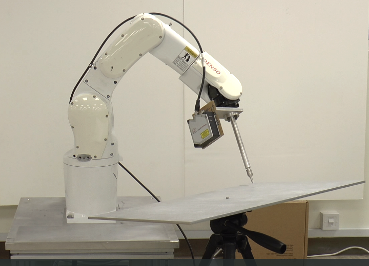
(a)

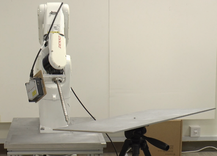
(b)

Figure 2: Distance constraints by moving the tool-tip linearly through a known distance.

To account for this problem, we need to add more constraints that only affect one of the two parameters sets – either the robot or the laser parameters. To achieve this, we move the robot’s end-effector between two points that have a known distance $D$ and use this as a distance constraint during the calibration optimization. The plate has a pair of holes separated at distance $D$, and a sharp tool-tip is attached on the robot’s flange. The robot is moved such that the tool-tip touches the first hole, see Fig. 2 LABEL:sub@subfig:constraints-a, and the robot’s joint angles are recorded. At this configuration, the tool-tip position can be computed as ${{}^{B}}{\bf\it t}_{l1}={{}^{B}}{\bf\it T}_{E,l1}\;{{}^{E}}{\bf\it t}$, where ${{}^{B}}{\bf\it t}_{l1}$ and ${{}^{E}}{\bf\it t}$ are the position of the tool-tip in the robot base and end-effector frame respectively, $l$ is the location index of the plane, and the subscript $1$ refers to the first hole. The robot is then moved to touch the second hole, see Fig. 2 LABEL:sub@subfig:constraints-b, while maintaining the same orientation, and the joint angles are recorded. The tool-tip position at this second configuration can be computed as ${{}^{B}}{\bf\it t}_{l2}={{}^{B}}{\bf\it T}_{E,l2}\;{{}^{E}}{\bf\it t}$.

Since the distance between the two is known as $D$, then the parameters $\Phi$ have to satisfy the following constraint:

$$f_{t}({\bf\it\Phi})=\sum_{l=1}^{L}(|{{}^{B}}{\bf\it t}_{l2}-{{}^{B}}{\bf\it t}_{l1}|-D)^{2}=0.$$ (2)

Note that only the robot’s kinematic parameters in ${\bf\it\Phi}$ are affected by the additional constraint, while the laser parameters in ${\bf\it\Phi}$ are not affected at all. This constraint is added as an additional term to the objective function, so the objective function in SCALAR is now defined as

$$f({\bf\it\Phi})=\sum_{k=1}^{2}\sum_{j=1}^{N}\sum_{i=1}^{M}({{{}^{B}}{\bf\it n}_{k}}^{T}\;{{}^{B}}{\bf\it p}_{ji}-{{}^{B}}l_{k})^{2}+\\ w\sum_{l=1}^{L}(|{{}^{B}}{\bf\it t}_{l2}-{{}^{B}}{\bf\it t}_{l1}|-D)^{2}$$ (3)

where $w$ is an introduced weight to scale the contribution of the distance constraints over the planar constraints. The value of $w$ has to be carefully chosen to balance the effect of the first and the second term in the objective function. In Section IV-B the optimal value of $w$ will be determined experimentally.

${\bf\it\Phi}$ consists of 24 DH parameters for a 6-DoF robot, 7 parameters for the laser’s parameters, and 8 parameters for the plane parameters at two locations. In total, there are 39 parameters to be optimized by minimizing the objective function $f({\bf\it\Phi})$. The optimization problem is then solved using a Levenberg-Marquardt nonlinear optimizer [27].

For the unit vector parameters $[r_{x}\quad r_{y}\quad r_{z}]$ and $[{{}^{B}}n_{k,x}\quad{{}^{B}}n_{k,y}\quad{{}^{B}}n_{k,z}]$, the following constraints are added to the optimization solver,

$${r_{z}}=\sqrt{1-{r_{x}}^{2}-{r_{y}}^{2}}$$ (4)

$${{}^{B}}n_{k,z}=\sqrt{1-{{{}^{B}}n_{k,x}}^{2}-{{{}^{B}}n_{k,y}}^{2}}$$ (5)

III-B Tool Calibration Procedure (Optional)

The additional distance constraint in Section III-A contains the term ${{}^{E}}{\bf\it t}=[t_{x}\quad t_{y}\quad t_{z}]$, which is the tool-tip coordinates in the end-effector frame. If the robot accurately maintains the tool-tip orientation while touching the pair of holes, the distances travelled by the robot’s flange and the tool-tip are actually the same since they are part of the same rigid body. In that case, an accurate value of ${{}^{E}}{\bf\it t}$ is not necessary.

However, this is true under the assumption that the end-effector orientation can be kept constant between the two hole positions. This largely depends on the accuracy of the initial robot kinematic parameters. If these parameters are far from the real ones, then the end-effector orientation might actually change significantly between the two holes. In this case, the error in ${{}^{E}}{\bf\it t}$ – computed using the initial robot kinematic parameters – will corrupt the calibration result, hence a more accurate value of ${{}^{E}}{\bf\it t}$ will be necessary. Several methods can be used to get such accurate value, e.g. using a Coordinate-Measuring Machine to measure ${{}^{E}}{\bf\it t}$ or using the information from the CAD models.

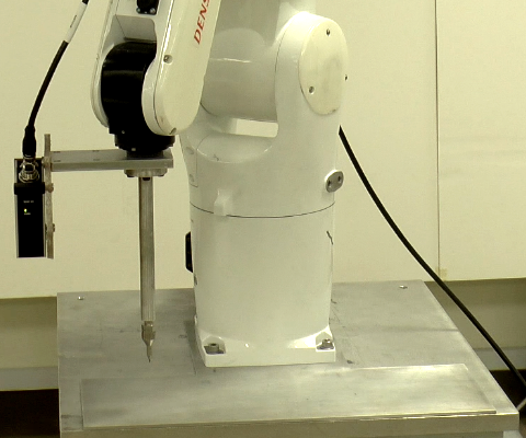
(a)

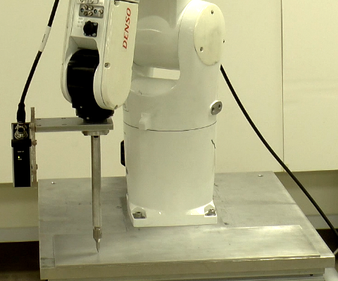
(b)

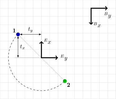
(c)

Figure 3: Tool Calibration

In this work, we use a simple calibration method to calibrate ${{}^{E}}{\bf\it t}$. A base plate with a small diameter hole is attached to the robot base. First the tool is oriented such that z-axis of the robot’s end-effector ${{}^{E}}\textbf{z}$ points to the opposite direction of the robot base’s z-axis ${{}^{B}}\textbf{z}$ (the vertical direction), see Fig. 3 LABEL:sub@subfig:tool-calib-a, while ${{}^{E}}\textbf{x}$ points to the opposite of ${{}^{B}}\textbf{x}$, and ${{}^{E}}\textbf{y}$ points to the same direction as ${{}^{B}}\textbf{y}$. Next, we move the robot such that the tool-tip touches the hole on the base plane, see Fig. 3 LABEL:sub@subfig:tool-calib-b, while maintaining its orientation. The z-coordinate of the hole is 0, because it is located on the robot base. From the robot’s kinematics, we can also get the z-coordinate of the robot’s flange. The difference between the two will give us the z-component of ${{}^{E}}{\bf\it t}$, which is $t_{z}$.

Next we need to find $t_{x}$ and $t_{y}$. To do that, when the robot is at the position in Fig. 3 LABEL:sub@subfig:tool-calib-b, the last joint of the robot is rotated by 180 degrees. That will cause the tool-tip to move semi-circularly in the horizontal plane. In Fig. 3 LABEL:sub@subfig:tool-calib-c, the center of the circle is the x-y coordinates of the robot’s flange, while the x-y coordinates of the tool-tip will traverse the circle as the last joint is rotated. Both coordinates are seen from the robot base frame (${{}^{B}}x$ and ${{}^{B}}y$). Initially, the tool-tip is at point 1 (which coincides with the hole on the base plane), and the coordinate frame of the robot flange is as indicated at the center (${{}^{E}}x$ and ${{}^{E}}y$). At this position, $t_{x}$ and $t_{y}$ are the same as the x and y coordinates of the point 1 in the robot’s flange coordinate frame which are still unknown. As the last joint is rotated 180 degrees, the tool-tip will move along the circle from point 1 to point 2. By calculating the shift in x and y direction between point 1 and point 2, $t_{x}$ and $t_{y}$ can be calculated. Since point 1 coincides with the hole, this shift can be measured by moving the tool-tip linearly without changing orientation from point 2 to point 1 using the robot’s teaching pendant, and record the change of the robot’s tool-tip position. From that we can obtain $t_{x}$ and $t_{y}$.

In the experiment section, we will demonstrate that the accurate tool calibration is not necessary in SCALAR if the robot’s initial DH parameters are quite accurate. Hence, we use this tool calibration mainly for the validation purpose. In actual calibration practice, the user can just do a rough measurement or use the information from the CAD model to obtain the tool-tip coordinates.

III-C Identifiability of the calibration parameters

In [3] we used three plate locations for the planar constraints based on the findings of Zhuang et al. [13]. However, we realize that two planes are actually sufficient for our method of calibration, due to the fact that we are using a 2D laser, whereas [13] used a touch probe. Unlike a touch probe which only gives a single point on the robot end-effector for calibration, 2D laser data gives us multiple data points with respect to the robot’s end-effector, and these points change at different poses. This result in fewer number of planes required for the calibration. Using the identifiability analysis here, we demonstrate that two planes are indeed enough for calibrating the same set of parameters as with three planes.

Following the approach in [16] and [28], SVD is applied on the identification Jacobian matrix ${\bf\it J}$. Let $f_{kji}(\Phi)$ be the geometric constraint equation on the data point $i$ at the robot pose $j$ and on the plane $k$,

$$f_{kji}({\bf\it\Phi})={{{}^{B}}{\bf\it n}_{k}}^{T}\;{{}^{B}}{\bf\it p}_{ji}-{{}^{B}}l_{k}=0\;.$$ (6)

Then ${\bf\it J}$ can be computed by differentiating (6) for all the data points $i=1,\cdots,M$ at the robot poses $j=1,\cdots,N$ and for all the planes $k=1,2$, then stack them together as a matrix, ${\bf\it J}=\begin{bmatrix}\frac{\partial f_{111}({\bf\it\Phi})}{\partial{\bf\it\Phi}}\quad\frac{\partial f_{112}({\bf\it\Phi})}{\partial{\bf\it\Phi}}\quad\cdots\quad\frac{\partial f_{2MN}({\bf\it\Phi})}{\partial{\bf\it\Phi}}\quad\end{bmatrix}^{T}\;.$ We can then apply SVD to the matrix ${\bf\it J}={\bf\it U}{\bf\it\Sigma}{\bf\it V}^{T}\;$.

For this identification step, the parameters $[r_{z}\quad{{}^{B}}n_{1,z}\quad{{}^{B}}n_{2,z}\quad]$ are excluded from the parameters vector ${\bf\it\Phi}$, since those three parameters are dependent on other parameters, see (4) and (5). That leaves us with $39-3=36$ parameters in ${\bf\it\Phi}$.

In this paper, we use a Denso VS060 6-DoF industrial manipulator with its DH parameters presented in the first column of Table I. The Jacobian ${\bf\it J}$ is computed by finite difference method. Applying the identifiability analysis to the system, we found that there are 7 sets of linearly dependent parameters out of the 36 parameters. These are exactly the same sets of parameters as found in [3], although here we use two plane locations ($k=2$) instead of three. For each set of the linearly dependent parameters, we can assign a fix value to one of the parameters. In this case, we fix the value of the parameters [$d_{6},\theta_{6},d_{2},a_{1},\alpha_{1},\theta_{1},d_{1}$] to their initial model’s values. More details can be found in [3].

Finally, we would like to note a few things:

• The reduction of the number of plane’s locations from three to two do not change the set of identifiable parameters (see [3] for the same analysis to three planes calibration). This validates our claim that two plane’s locations are sufficient for calibration using a 2D laser.

• In this analysis, we only make use of the planar constraints to analyse the identifiable parameters. This means that theoretically the planar constraints are sufficient for the calibration purpose, although not practically due to the various sources of errors (laser data error, flatness error, robot’s stiffness, etc), resulting in a slight dependency between the robot’s and the laser’s parameters during optimization. Including the distance constraint in the identifiability analysis will give us the same result in terms of the set of identifiable parameters.

• These results apply to most existing 6-DoF industrial robots whose kinematic structures are similar to our Denso robot. Moreover, the analysis can be extended to any robot with arbitrary kinematic structures.

IV Experimental Result

The experimental setup can be seen in Fig. 1. We use the following equipment:

• DENSO VS060 6-DoF industrial robot arm.

• Micro-Epsilon scanControl 2600-100 2D LRF, attached on the robot’s flange. The LRF has $100$ mm optimum range and $300$ mm maximum range, with $0.012$ mm accuracy in its z-direction. The optimum range is used here for better accuracy.

• A custom tool, attached to the robot’s flange. The diameter of the tool-tip is less than $0.1$ mm.

• A base plate, attached below the robot’s base. The plate has holes with $0.3$ mm diameter and $0.3$ mm depth.

• An aluminium plate with flatness within $0.05$ mm. There are a pair of holes with $0.3$ mm diameter and $0.3$ mm depth on the plate. The holes are separated at $D\leavevmode\nobreak\ =\leavevmode\nobreak\ 500$ mm distance with $0.01$ mm tolerance. $D$ is chosen to be as large as possible such that small errors in robot’s and laser’s parameters result in large tool-tip distance errors.

In addition, we also use FARO Edge Arm as an additional validation tool for SCALAR. It can measure XYZ positions within $0.05$ mm accuracy. Note that this tool is only used to further validate SCALAR, and it is not required in the actual calibration procedure.

The calibration procedure during the experiment is as follows. First, the aluminium plate is placed at two different locations in the robot’s workspace. For each location, the robot is moved to $N=50$ different poses such that the LRF’s ray intersects the plate at each pose. The robot’s joint angles and the laser data are recorded. This gives us 100 poses, 60 of which will be used for calibration (as proposed in [3]) while the remaining 40 poses are used for validation. The value of $M$ is chosen as 40.

Next, the plate is moved to 50 different locations, and the robot is moved such that the tool-tip touches the pair of holes on the plate consecutively without changing orientation. The robot’s joint angles are recorded. This gives us 50 pair of joint angles, 15 of which will be used for calibration and 35 will be used for validation.

Finally, the tool-tip position is calibrated using the hole at the base plate, as explained in Section III-B.

The following subsections will be as follows. Section IV-A explains the three methods for validating the calibration result. In Section IV-B the optimal value for $w$ is determined experimentally. Section IV-C presents the general result obtained by SCALAR. In Section IV-D, Section IV-E, and Section IV-F, we compare the performance of SCALAR against three other cases:

• Nominal DH. In this case, we run the whole calibration procedure, but we only optimize the laser parameters and the plane parameters while keeping the DH parameters to the nominal value, which is obtained from the manufacturer.

• Noisy DH. Similar to the Nominal DH, but here we fix the noisy (instead of nominal) DH parameters while optimizing all the other parameters. The noisy DH parameters are generated by introducing random errors to the nominal DH parameters within the range of $\pm 2$ mm for linear parameters and $\pm 1$ degrees for angular parameters.

• SCALAR_α. In this case, we use only the planar constraint in the objective function as in [3].

In Section IV-G, we analyse the effect of the tool calibration error to the SCALAR calibration result. We claim that the tool calibration does not need to be very accurate in order for SCALAR to yield a good result. This means that we can even skip the tool calibration and just use the nominal tool-tip parameters from the CAD model or some rough measurement. Finally, in Section IV-H we discuss some of the interesting points from the experimental results.

IV-A Validation Method

In this paper, the planar error is defined as the error of the laser data points with respect to the plane, and can be calculated by the following formula,

$$\delta_{p}=|{{{}^{B}}{\bf\it n}_{k}}^{T}\cdot{{}^{B}}{\bf\it p}_{ji}-{{}^{B}}l_{k}|\quad.$$ (7)

The tool-tip distance error is defined as the difference between the distance travelled by the tool-tip when it touches the pair of holes according to the DH parameters and according to the known value ($D$), and it is calculated by the following formula,

$$\delta_{t}=||{{}^{B}}{\bf\it t}_{l2}-{{}^{B}}{\bf\it t}_{l1}|-D|\quad.$$ (8)

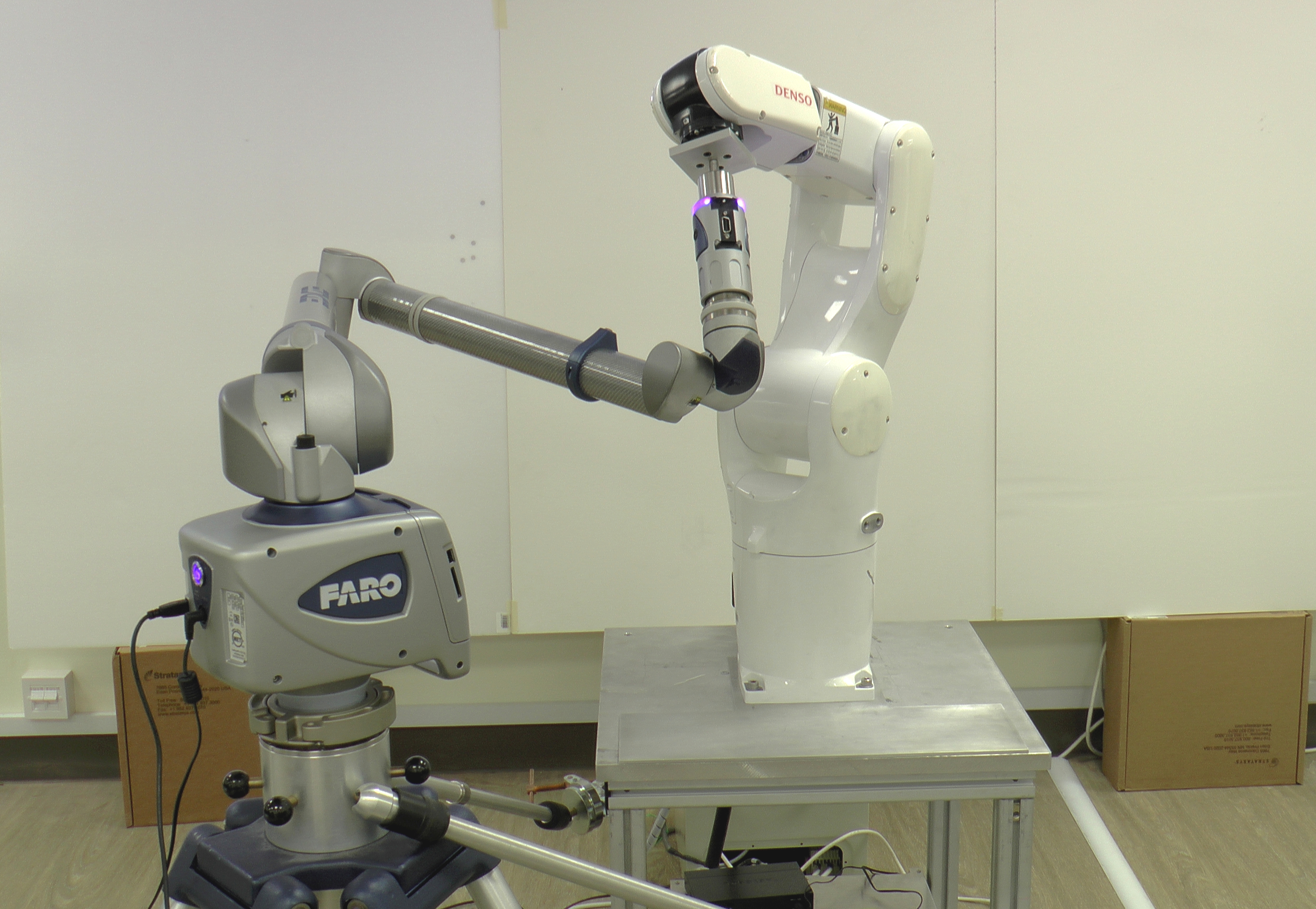
Figure 4: FARO Edge Arm is used as the third method to validate the calibration result

The planar error and the tool-tip distance errors will be used for validating the calibration method.

The validation using the tool-tip distance error involves only the tool-tip and the holes on the plate, so it does not require additional equipment. However, the certainty provided by this validation method is limited by the size of the holes and by how much the human eye can differentiate the tool-tip position. To validate the calibration result with more certainty, we use a FARO Edge Arm as the third validation method. The device can measure its end-point very accurately within $0.05$ mm. The end-point is rigidly attached to the robot’s flange, as depicted in Fig. 4. The validation process here is similar to the second method with the tool-tip; the robot is moved to two different poses without changing the orientation. The distance between the two poses, $D$, is measured by the FARO arm, and it is compared with the distance calculated based on the DH parameters. FARO distance error is defined as

$$\delta_{f}=||{{}^{B}}T_{E,2}{{}^{E}}{\bf\it o}-{{}^{B}}T_{E,1}{{}^{E}}{\bf\it o}|-D|\quad$$ (9)

where ${{}^{B}}T_{E,2}$ and ${{}^{B}}T_{E,1}$ refer to the two poses of end-effector with the same orientation and ${{}^{E}}{\bf\it o}$ refers to the zero position vector (the origin of the end-effector frame).

We use the mean, the standard deviation, and the maximum of $\delta_{p}$, $\delta_{t}$, and $\delta_{f}$ to validate the proposed calibration method. For validation, we use 40 poses at two plate’s locations for the calculation of $\delta_{p}$, 35 plate’s locations for $\delta_{t}$ and 50 pair of robot poses for $\delta_{f}$.

Table I: Comparison of the parameters: Nominal, Noisy, SCALAR_α and SCALAR

Parameter	Nominal	Noisy	SCALARα	SCALAR+
${\alpha}_{1}$	0.00	0.00	0.00	0.00
$a_{1}$	0.00	0.00	0.00	0.00
${\theta}_{1}$	0.00	0.00	0.00	0.00
$d_{1}$	345.00	345.00	345.00	345.00
${\alpha}_{2}$	-90.00	-90.17	-89.94	-89.92
$a_{2}$	0.00	-2.00	-0.05	0.17
${\theta}_{2}$	-90.00	-89.56	-90.01	-89.97
$d_{2}$	0.00	-0.79	-0.79	-0.79
${\alpha}_{3}$	0.00	-0.71	0.01	0.01
$a_{3}$	305.00	303.75	305.42	305.07
${\theta}_{3}$	90.00	89.18	90.01	90.01
$d_{3}$	0.00	-0.62	1.04	1.01
${\alpha}_{4}$	90.00	89.79	89.95	89.97
$a_{4}$	-10.00	-10.32	-9.82	-9.83
${\theta}_{4}$	0.00	-1.57	-0.15	-0.15
$d_{4}$	300.00	300.74	300.05	299.61
${\alpha}_{5}$	-90.00	-90.59	-89.96	-89.97
$a_{5}$	0.00	-1.89	0.25	0.22
${\theta}_{5}$	0.00	0.76	0.04	0.03
$d_{5}$	0.00	0.68	-0.37	-0.24
${\alpha}_{6}$	90.00	90.00	89.94	89.96
$a_{6}$	0.00	0.00	0.04	0.08
${\theta}_{6}$	0.00	0.00	0.00	0.00
$d_{6}$	70.00	70.00	70.00	70.00
$p_{x}$	-127.50	-127.50	-125.46	-125.26
$p_{y}$	-33.00	-33.00	-33.92	-34.04
$p_{z}$	101.50	101.50	99.35	99.01
$r_{x}$	0.00	0.00	-0.00	-0.00
$r_{y}$	0.00	0.00	-0.00	-0.00
$r_{z}$	1.00	1.00	1.00	1.00
$r_{w}$	3.14	3.14	3.13	3.13
$n_{1,x}$	0.00	0.00	-0.01	-0.01
$n_{1,y}$	0.00	0.00	-0.04	-0.04
$n_{1,z}$	1.00	1.00	1.00	1.00
$l_{1}$	0.00	0.00	-83.97	-84.17
$n_{2,x}$	0.00	0.00	-0.01	-0.01
$n_{2,y}$	1.00	1.00	1.00	1.00
$n_{2,z}$	0.00	0.00	0.00	0.00
$l_{2}$	600.00	600.00	819.79	818.91

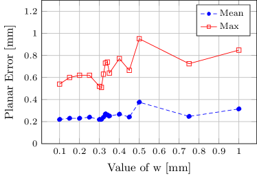
(a)

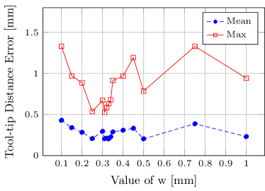
(b)

Figure 5: The effect of the weight $w$ on: a) Planar Error, and b) Tool-tip Distance Error

Table II: Comparing SCALAR Result with the other cases (in mm)

Parameter	Planar Errors			Tool-tip Distance Errors			Faro Distance Errors
	Mean	Std	Max	Mean	Std	Max	Mean	Std	Max
Nominal DH	0.53	0.58	1.13	0.741	0.736	1.424	0.44	0.34	1.4
Noisy DH	3.92	3.96	7.76	3.25	3.73	7.51	2.67	1.70	8.97
SCALARα	0.20	0.22	0.46	0.664	0.608	1.338	0.34	0.26	1.45
SCALAR	0.23	0.25	0.59	0.24	0.27	0.50	0.19	0.13	0.50

IV-B Determining the weight $w$

The weight $w$ in the SCALAR objective function (3) determines the relative effect of the additional distance constraints term in the optimization. If $w$ is too small, the distance term will be dominated by the planar term, and the objective function will be reduced to the SCALAR_α objective function (1). If $w$ is too large, the distance term will dominate and the optimization result will be sub-optimal. To determine the optimal value of $w$, the optimization is run while varying the value of $w$, and the result is compared in terms of the planar error and the tool-tip distance error. Fig. 5 LABEL:sub@subfig:plane and Fig. 5 LABEL:sub@subfig:point show the effect of $w$ to the planar error and the tool-tip distance error, respectively. Note that when the value of $w$ is small, the planar error is small but the tool-tip distance error is large (this corresponds to SCALAR_α result). As $w$ is increased, the planar error increases slightly but the tool-tip distance error decreases, with its lowest point around $w$ = 0.31. As $w$ is increased further, both the planar error and the tool-tip distance error increase. Hence, $w$ = 0.31 is chosen as the optimal weight for all subsequent experiments.

IV-C General Result

Table I shows the comparison between the nominal parameters, the noisy parameters, and the calibrated parameters from SCALAR_α and SCALAR. The noisy parameters are used as the initial values for SCALAR_α and SCALAR. It can be seen from the table that although the noisy DH parameters are far from the nominal ones, SCALAR_α and SCALAR calibrate the DH parameters to be very close to the nominal ones. This is important because the nominal DH Parameters are already quite accurate (as will be shown in the following sections). On the contrary, the calibrated plane parameters are very different from the nominal and noisy ones, which demonstrate that accurate initial estimate of the plane parameters are not required in SCALAR.

After calibration, SCALAR results in $0.23$ mm mean planar error, $0.24$ mm mean tool-tip distance error, and $0.19$ mm mean FARO distance error, which are better than the Nominal DH and SCALAR$\alpha$ case. The optimization converges in less than 15 iterations with the total residual (Eq. 3) less than $10^{-6}\leavevmode\nobreak\ m^{2}$.

Hayati et al. [29] established that in the case of two parallel consecutive joints, the DH parameters are singular w.r.t. calibration. This means that a slight shift from the parallel configuration in the actual joint location results in large changes to the singular DH parameters. The second and third joint of the robot are parallel in our case, so this case should be considered as singular. Several ways have been proposed to account for this singularity, including [29]. However, we realized that by fixing the parameter $d_{2}$ (as a result of the identifiability analysis in Section III-C), the singularity problem actually disappears. Fixing $d_{2}$ corresponds to forcing the location of the second joint to be near the original location, preventing the other set of DH parameters to change significantly. We also tried using the modified DH parameters [29], and the results that we obtained are similar to the ones presented here with standard DH parameters.

IV-D Comparison of Planar Errors

The first three columns of Table II show the the planar error comparison. While Noisy DH gives very large errors, SCALAR_α and SCALAR improve the parameters such that the errors are even better than the Nominal DH. This demonstrates that both methods are able to improve the parameters of the robot and the laser as a whole such that the prediction of the laser data position can be obtained accurately. SCALAR_α has slightly better result as compared to SCALAR, which is expected since the only objective function in SCALAR_α is the planar error.

IV-E Comparison of Tool-tip Distance Errors

The middle columns of Table II show the the tool-tip distance error comparison. SCALAR has the lowest errors, while SCALAR_α has similar errors compared to the Nominal DH. To explain this, note that the tool-tip distance error only depends on the robot’s kinematic parameters and not on the laser parameters. This demonstrates that although SCALAR can optimize the combined robot kinematic parameters and laser parameters to achieve good estimates for the laser data points w.r.t. the robot’s base frame, the robot kinematic parameters and the laser’s extrinsic parameters, independently, are not optimal. In other words, SCALAR_α modifies the kinematic parameters and the laser parameters such that the combination minimizes the planar error, but the kinematic parameters by itself do not predict properly the robot’s end-effector pose. By adding the distance constraint to the objective function in SCALAR, the end-effector pose is predicted more accurately.

IV-F Comparison of FARO Distance Error

To further validate the calibration result, we use the FARO arm to measure the distance $D$ travelled by the robot’s end-effector. In contrast to Section IV-E, here the distance $D$ is not constant. The measured distance is then compared with the calculated distance based on the DH parameters, which gives us the FARO distance error. The comparison result is shown in the last three columns of Table II. The noisy DH parameters give very high errors w.r.t. the FARO measurement, with $8.97$ mm as the maximum error. The mean error of the nominal DH parameters is low, around $0.44$ mm, but the maximum error is up to $1.41$ mm. SCALAR_α only improves the mean and standard deviation of the error to be slightly better as compared to the nominal parameters. In contrast, SCALAR manages to improve the mean, standard deviation, and maximum error significantly.

Here we emphasize that the conclusions obtained by looking at FARO distance error and at tool-tip distance error are very similar: SCALAR outperforms SCALAR_α in improving the robot’s end-effector pose prediction. This shows that at the absence of expensive equipment such as FARO arm, the calibration and its validation can still be performed with good confidence.

Figure 6: The effect of the tool-tip calibration error to the distance error

IV-G Effect of the tool-tip calibration error

In this section, we demonstrate that accurate tool-tip calibration is not necessary for SCALAR to successfully improve the kinematic and laser parameters. To do that, we consider the calibrated tool-tip coordinates, see Section III-C, to be the true tool-tip coordinates, and we introduce errors separately to the x, y, and z coordinates of the tool-tip, ranging from $0.5$ mm to $50$ mm. The modified tool-tip coordinates are used in SCALAR for calibration. The calibrated kinematic parameters are then validated against the FARO measurement by calculating the FARO distance errors such as in Section IV-F.

Fig. 6 show the effect of the tool-tip coordinates error in x, y, and z coordinate to the FARO distance error. It is clear that the errors in tool-tip coordinates do not affect the FARO distance error significantly. This is due to the fact that when the robot is moved to touch the pair of holes on the plate, we keep the orientation of the robot constant, at least according to the initial DH parameters. When the orientation is constant, the distance travelled by the robot flange is the same as the distance travelled by the tool-tip, or any point which is rigidly attached to the robot’s flange. This means that the tool-tip coordinates do not affect the tool-tip distance error at all.

However, it is important to note that in practice when we move the robot to touch the pair of holes, we usually depend on the robot’s teach pendant to maintain the constant orientation of the robot. Since the robot’s teach pendant uses the nominal DH parameters which have some errors, the actual orientation may actually change between the two robot poses, even though the teach pendant shows the two orientations to be the same. If the actual change in orientation is large, the tool-tip coordinates errors can have a significant effect on the calibration result. The change in orientation will be propagated by the tool-tip coordinate error to result in the tool-tip position error. In such cases, tool-tip calibration is necessary.

To evaluate the effect of orientation errors on the tool-tip position, we can use a simple trigonometry equation which relates the magnitude of an angle to the length of an arc,

$${\epsilon}_{x}={\epsilon}_{\theta}\cdot{\epsilon}_{t}\quad,$$ (10)

where ${\epsilon}_{x}$ is the change in tool-tip position, ${\epsilon}_{\theta}$ is the change in tool-tip orientation, and ${\epsilon}_{t}$ is the error in tool-tip coordinates. From this formula, given the initial robot orientation accuracy and the acceptable error in tool-tip position, we can calculate the tolerable tool-tip coordinate errors. For example, if the negligible change in tool-tip position is $0.05$ mm, and the error in robot orientation is $0.02$ rad ($1.15$ degrees), the acceptable error in tool-tip coordinates is $2.5$ mm. This means that $2.5$ mm errors in tool-tip coordinates will only result in $0.05$ mm error of the tool-tip position for a robot with orientation accuracy around $1$ degree.

IV-H Discussion

Based on the experiments that we conducted, we note the followings:

• The laser accuracy depends on the plate’s surface. Our plate is made of aluminium, which gives quite a lot of noise to the laser data (within the range of $0.1$ mm). If the plate can be made of other materials with less specularity, the calibration result can be further improved.

• The validation using the holes on the plate give us similar result to the validation using FARO Edge Arm. This means that in practice we can rely on the validation using the holes with confidence.

• The addition of tool-tip errors to the objective function indeed results in more inconvenience, as the data collection for this step requires manual intervention. However, only 15 pair of points are required for calibration, so the manual step can be completed quite fast (typically within 10-15 minutes). In addition, the distance constraint is not necessary if we only want to calibrate one of the two parameters set (either the robot’s the laser’s parameters)

• Instead of using 2D LRF, it is possible to use two or more pieces of 1D LRF which are rigidly attached to the robot. This will cost even cheaper as compared to 2D LRF, although more calibration poses might be necessary.

• We demonstrate that using two plate’s locations instead of three is sufficient. The calibration algorithm can use more plate’s locations so that the range of the workspace explored by the calibration is extended, but we found that the result using more plate’s locations is similar to that obtained by two plate’s locations.

• In this work we do not try to find the optimal set of calibration poses, but instead rely on the random poses to cover the robot’s configuration space. There are a lot of methods that have been proposed to find such an optimal set, e.g. using the singular values of the Jacobian or the information matrix ( [28],[30]). [31] use the parameters covariance matrix to determine the next-best-pose.

V Conclusions

In this paper, we have proposed SCALAR, a novel method to calibrate simultaneously a 6-DoF industrial robot’s kinematic parameters and a 2D LRF extrinsic parameters. SCALAR has been shown to be an improvement over our previous method (SCALAR_α), since it finds the optimal parameters for each set (robot and laser). SCALAR reduces the mean planar errors from $0.53$ mm to around $0.23$ mm, the mean tool-tip distance errors from $0.74$ mm to $0.24$ mm, and the FARO distance errors from $0.44$ mm to $0.19$ mm. The proposed method is inexpensive and convenient, as it does not require expensive external measurement systems or an elaborated calibration setting.

References

- [1] X. Zhang, M. Li, J. H. Lim, Y. Weng, Y. W. D. Tay, H. Pham, and Q.-C. Pham, “Large-scale 3d printing by a team of mobile robots,” Automation in Construction, vol. 95, pp. 98–106, 2018.
- [2] F. Suárez-Ruiz, T. Santoso Lembono, and Q.-C. Pham, “RoboTSP – A Fast Solution to the Robotic Task Sequencing Problem,” in IEEE Int. Conf. on Robotics and Automation, 2018.
- [3] T. S. Lembono, F. Suárez-Ruiz, and Q. C. Pham, “SCALAR - Simultaneous Calibration of 2D Laser and Robot’s Kinematic Parameters Using Three Planar Constraints,” in IEEE/RSJ Int. Conf. on Intelligent Robots and Systems, 2018.
- [4] S. H. Ye, Y. Wang, Y. J. Ren, and D. K. Li, “Robot calibration using iteration and differential kinematics,” Journal of Physics: Conference Series, vol. 48, no. 1, pp. 1–6, 2006.
- [5] L. S. Ginani and J. M. S. T. Motta, “Theoretical and practical aspects of robot calibration with experimental verification,” Journal of the Brazilian Society of Mechanical Sciences and Engineering, vol. 33, no. 1, pp. 15–21, 2011.
- [6] A. Nubiola and I. A. Bonev, “Absolute calibration of an ABB IRB 1600 robot using a laser tracker,” Robotics and Computer-Integrated Manufacturing, vol. 29, no. 1, pp. 236–245, 2013.
- [7] L. Wu and H. Ren, “Finding the Kinematic Base Frame of a Robot by Hand-Eye Calibration Using 3D Position Data,” IEEE Transactions on Automation Science and Engineering, vol. 14, no. 1, pp. 314–324, 2017.
- [8] C. S. Gatla, R. Lumia, J. Wood, and G. Starr, “An automated method to calibrate industrial robots using a virtual closed kinematic chain,” IEEE Transactions on Robotics, vol. 23, no. 6, pp. 1105–1116, 2007.
- [9] Y.-J. Chiu and M.-H. Perng, “Self-calibration of a general hexapod manipulator using cylinder constraints,” International Journal of Machine Tools and Manufacture, vol. 43, pp. 1051–1066, 2003.
- [10] X. L. Zhong and J. M. Lewis, “New method for autonomous robot calibration,” IEEE Int. Conf. on Robotics and Automation, vol. 2, pp. 1790–1795, 1995.
- [11] X. L. Zhong, J. M. Lewis, and F. L. N. Nagy, “Autonomous robot calibration using a trigger probe,” Robotics and Autonomous Systems, vol. 18, no. 4, pp. 395–410, 1996.
- [12] M. Ikits and J. Hollerbach, “Kinematic calibration using a plane constraint,” IEEE Int. Conf. on Robotics and Automation, vol. 2, no. 4, pp. 3191–3196, 1997.
- [13] Z. Hanqi, S. Motaghedi, and Z. Roth, “Robot calibration with planar constraints,” IEEE Int. Conf. on Robotics and Automation, vol. 1, pp. 1–25, 1999.
- [14] T. Zilong, N. Zhanhai, and L. Xinggang, “Autonomous calibration research of polishing robot,” Proceedings of the World Congress on Intelligent Control and Automation (WCICA), vol. 2, pp. 8938–8942, 2006.
- [15] H. Hage, P. Bidaud, and N. Jardin, “Practical consideration on the identification of the kinematic parameters of the St¨aubli TX90 robot,” World, pp. 19–25, 2011.
- [16] A. Joubair and I. A. Bonev, “Non-kinematic calibration of a six-axis serial robot using planar constraints,” Precision Engineering, vol. 40, pp. 325–333, 2015.
- [17] W. Wang, A. Li, and D. Wu, “Robot calibration by observing a virtual fixed point,” in IEEE International Conference on Robotics and Biomimetics (ROBIO), Dec 2009, pp. 1351–1355.
- [18] Y. Liu, N. Xi, G. Zhang, X. Li, H. Chen, C. Zhang, M. J. Jeffery, and T. A. Fuhlbrigge, “An automated method to calibrate industrial robot joint offset using virtual line-based single-point constraint approach,” in IEEE/RSJ Int. Conf. on Intelligent Robots and Systems, 2009, pp. 715–720.
- [19] Y. Liu and N. Xi, “Low-cost and automated calibration method for joint offset of industrial robot using single-point constraint,” Industrial Robot, vol. 38, no. 6, pp. 577–584, 2011.
- [20] A. Joubair and I. A. Bonev, “Kinematic calibration of a six-axis serial robot using distance and sphere constraints,” The International Journal of Advanced Manufacturing Technology, vol. 77, no. 1-4, pp. 515–523, 2015.
- [21] C. L. Choi, J. Rebello, L. Koppel, P. Ganti, A. Das, and S. L. Waslander, “Encoderless gimbal calibration of dynamic multi-camera clusters,” in IEEE Int. Conf. on Robotics and Automation, May 2018, pp. 2126–2133.
- [22] A. Das, “Informed data selection for dynamic multi-camera clusters,” Ph.D. dissertation, University of Waterloo, 2018.
- [23] Qilong Zhang and R. Pless, “Extrinsic calibration of a camera and laser range finder (improves camera calibration),” in IEEE/RSJ Int. Conf. on Intelligent Robots and Systems, vol. 3, 2004, pp. 2301–2306.
- [24] R. Unnikrishnan and M. Hebert, “Fast Extrinsic Calibration of a Laser Rangefinder to a Camera,” Robotics, 2005.
- [25] W. Chen, J. Du, W. Xiong, Y. Wang, S. Chia, B. Liu, J. Cheng, and Y. Gu, “A Noise-Tolerant Algorithm for Robot-Sensor Calibration Using a Planar Disk of Arbitrary 3-D Orientation,” IEEE Transactions on Automation Science and Engineering, vol. 15, no. 1, pp. 251–263, 2018.
- [26] Y. Li, W. Zhang, J. Cao, J. Peng, B. Jiang, and L. Wang, “3D laser scanner calibration method based on invasive weed optimization and Levenberg-Marquardt algorithm,” in IEEE Int. Conf. on Automation Science and Engineering, 2017, pp. 1280–1285.
- [27] M. Newville, T. Stensitzki, D. B. Allen, and A. Ingargiola, “LMFIT: Non-Linear Least-Square Minimization and Curve-Fitting for Python,” 2014.
- [28] J. M. Hollerbach and C. W. Wampler, “The calibration index and taxonomy for robot kinematic calibration methods,” International Journal of Robotics Research, vol. 15, no. 6, pp. 573–591, 1996.
- [29] S. Hayati and M. Mirmirani, “Improving the absolute positioning accuracy of robot manipulators,” Journal of Robotic Systems, vol. 2, no. 4, pp. 397–413, 1985.
- [30] G. Xiong, Y. Ding, L. Zhu, and C.-Y. Su, “A product-of-exponential-based robot calibration method with optimal measurement configurations,” International Journal of Advanced Robotic Systems, vol. 14, no. 6, 2017.
- [31] J. Rebello, A. Das, and S. Waslander, “Autonomous active calibration of a dynamic camera cluster using next-best-view,” in IEEE/RSJ Int. Conf. on Intelligent Robots and Systems, 2017, pp. 1484–1489.