Classification of the solutions of a mixed nonlinear Schrödinger system

Abstract

In this paper, we study a couple of NLS equations characterized by mixed cubic and superlinear power laws. Classification of the solutions as well as existence and uniqueness of the steady state solutions have been investigated.

1 Introduction

The paper is devoted to the study of some nonlinear systems of PDEs of the form

$$\cases{}{L}_{1}(u)+f_{1}(u,v)=0,\\ \mathcal{L}_{2}(v)+f_{2}(u,v)=0$$ (1)

where $u=u(x,t)$, $v=v(x,t)$ on a domain $\Omega\times(t_{0},+\infty)$, $\Omega\subset\mathbb{R}^{N}$, $t_{0}\in\mathbb{R}$ with suitable initial and boundary conditions. The operators $\mathcal{L}_{1}$ and $\mathcal{L}_{2}$ are linear Schrödinger-type operators of the form

$$\mathcal{L}_{i}(u(x,t))=iu_{t}+\sigma_{i}u_{xx},\;i=1,2$$

leading to a nonlinear Schrödinger system. $u_{xx}$ is the second order partial derivative relatively to $x$, which plays the role of the Laplacian, $u_{t}$ is the first order partial derivative in time, $\sigma_{i}$, $i=1,2$ are constant real positive parameters. $f_{1}$ and $f_{2}$ are nonlinear continuous functions of two variables.

Remark that whenever the $\mathcal{L}_{i}$’s are the classical Schrödinger operators

$$\mathcal{L}_{1}(u)=\mathcal{L}_{2}(u)=iu_{t}+u_{xx}$$

and $u=v=\varphi$, $f_{1}=f_{2}=f$, we come back to the original Schrödinger equation

$$i\varphi_{t}+\Delta\varphi=f(\varphi).$$ (2)

On the other hand, this last equation itself may lead to a system of PDEs of real valued functions satisfying a Heat system. Indeed, let $\varphi=u+iv=(1+i)u$, we get a system of coupled Heat ones

$$\cases{u}_{t}-\Delta u+f_{1}(u,v)=0.\\ v_{t}+\Delta v+f_{2}(u,v)=0,$$ (3)

where $f_{1}$ and $f_{2}$ are issued from the real and imagiary parts of $f(\varphi)$.

Return again to the system (1) in the simple case $\sigma_{i}=1$ and denote $\varphi=u+iv$ and $f(\varphi)=f_{1}(u,v)+if_{2}(u,v)$, we come back to the classical NLS equation where $u$ and $v$ may be seen as real and imaginary parts of the solution $\varphi$ of an equation of the form (2).

As it is related to many physical/natural phenomena such as plasma, optics, condensed matter physics, etc, nonlinear Schrödinger system has attracted the interest of researchers in different fields such as pure and applied mathematics, pure and applied physics, quantum mechanics, mathematical physics, and it continues to attract resaerchers nowadays with the discovery of nano-physics, fractal domains, planets understanding, … etc. For instence, in hydrodynamics, the NLS system may be a good model to describe the propagation of packets of waves according to some directions where a phenomenon of overlopping group velocity projection may occur [20]. In optics also, the propagation of short pulses has been investigated via a system of NLS equations [28].

In single NLS equation, studies have been well developed from both theoretical and numerical aspects. The most recent mixed model is developed in [8], [9], [10], [11], [12], [13], [14], [15], [24], [25], [27], [29], [41], [42], … with a general model

$$f(u)=|u|^{p-1}u+\lambda|u|^{q-1}u.$$

which coincides with $f(u,u)$ in the model (4). An extending interesting model will be a mixed model of nonlinearities

$$f(u,v)=(|u|^{p-1}+\lambda|v|^{q-1})u,\;\;p,q,\lambda\in\mathbb{R}.$$ (4)

In the literature, few works are done on such a model and are focusing on the mixed cubic-cubic ($p=q=3$) one

$$f(u,v)=(|u|^{2}+\lambda|v|^{2})u.$$

For example, in [43], (2+1)-dimensional coupled NLS equations have been studied based on symbolic computation and Hirota method via the cubic-cubic nonlinear system

$$\left\{\begin{array}[]{lll}iu_{t}+u_{xx}+\sigma(|u|^{2}+\alpha|v|^{2})u=0,\\ iv_{t}+v_{xx}+\sigma(|v|^{2}+\alpha|u|^{2})v=0,\end{array}\right.$$ (5)

where $\alpha$ and $\sigma$ are real parameters. The same system has been also studied by many authors such as [1], [19], [22], [23], [30], [39]. In [44], the following more general system has been investigated for the asymptotic time behavior of the solutions,

$$\left\{\begin{array}[]{lll}i\partial_{t}u+\alpha\partial_{x}^{2}u+A(|u|^{2}+|v|^{2})u=0,\\ i\partial_{t}v+\alpha\partial_{x}^{2}v+A(|u|^{2}+|v|^{2})v=0\\ \end{array}\right.$$ (6)

See also [21]. In [18] the following $p$-Laplacian stationary system has been discussed for necessary and sufficient conditions for the existence of the solutions

$$\left\{\begin{array}[]{c}-\Delta_{p}u=\mu_{1}\Gamma_{1}(x,u,v)~{}~{}\hbox{in}~{}~{}\mathbb{R}^{N}\\ -\Delta_{p}v=\mu_{2}\Gamma_{2}(x,u,v)~{}~{}\hbox{in}~{}~{}\mathbb{R}^{N},\end{array}\right.$$ (7)

where $\Delta_{p}u=div(|\nabla u|^{p-2}\nabla u)$ is the $p$-Laplacian $(1<p<N)$. In [6], solutions of the type

$$u(x,t)=u(x)e^{iwt},$$ (8)

where $u$ is a real function known as standing wave or steady state and $w\in\mathbb{R}$ has been investigated leading to the time-independent problem

$$-\Delta u+(m_{0}^{2}-\omega^{2})u-|u|^{p-2}u=0$$ (9)

See also [40]. Already with the familiar cubic-cubic case, numerical solutions have been developed in [45] for the one-dimensional system

$$\left\{\begin{array}[]{l}i\frac{\partial u}{\partial t}+\frac{1}{2}\frac{\partial^{2}u}{\partial x^{2}}+(|u|^{2}+\beta|v|^{2})u=0,\\ i\frac{\partial v}{\partial t}+\frac{1}{2}\frac{\partial^{2}v}{\partial x^{2}}+(\beta|u|^{2}+|v|^{2})v=0,\\ u(x,0)=u_{0}(x)~{}~{}~{}~{}~{}~{}v(x,0)=v_{0}(x).\end{array}\right.$$ (10)

on $\mathbb{R}$, where $u$ and $v$ stands for the wave amplitude considered in two polarizations. The parameter $\beta$ is related to phase modulation. $u_{0}$ and $v_{0}$ are fixed functions assumed to be sufficiently regular.

Coupled NLS system has been analyzed for symmetries and exact solutions in [34]. The problem studied is related to atmospheric gravity waves governed by the following general coupled NLS system.

$$\left\{\begin{array}[]{l}iu_{t}+\alpha_{1}u_{xx}+(\sigma_{1}|u|^{2}+\Gamma_{1}|v|^{2})u=0,\\ iv_{t}+iCv_{x}+\alpha_{2}v_{xx}+(\Gamma_{2}|u|^{2}+\sigma_{2}|v|^{2})v=0.\end{array}\right.$$ (11)

It is noticed that such a problem may be transformed to the wall known Boussinesq equation.

In [2], novel effective approach for systems of coupled NLS equations has been developed for the model problem

$$\left\{\begin{array}[]{lll}iu_{t}+iu_{x}+u_{xx}+u+v+\sigma_{1}f(u,v)u=0,\\ iv_{t}-iv_{x}+v_{xx}+u-v+\sigma_{2}g(u,v)v=0,\end{array}\right.$$ (12)

where $f$ and $g$ are smooth nonlinear real functions depending on $(|u|^{2},|v|^{2})$ and $\sigma_{1}$, $\sigma_{2}$ are parameters. In [33], the folowing nonlinear cubic-quintic and coupling quintic system of NLS equations has been examined,

$$\left\{\begin{array}[]{lll}u_{t}+m_{1}u_{xx}=(\alpha+i\beta)u+f_{1}|u|^{2}u+f_{2}|u|^{4}u+f_{3}|v|^{2}u+f_{4}|u|^{2}|v|^{2}u,\\ v_{t}+m_{2}v_{xx}=(\gamma+i\delta)v+g_{1}|v|^{2}v+g_{2}|v|^{4}v+g_{3}|u|^{2}v+g_{4}|u|^{2}|v|^{2}v,\\ \end{array}\right.$$ (13)

where $u$ and $v$ describe the complex envelopes of an electric field in a co-moving frame. $\alpha$ and $\gamma$ are potentials. $\beta$ and $\delta$ are amplifications. The functions $f_{j}$ and $g_{j}$, $j=1,1,3,4$ describe the cubic, quintic and coupling quintic nonlinearities coefficients respectively. $m_{1}$ and $m_{2}$ stands for the dispersion parameters

In [26], existence of ground state solutions has been studied for the NLS system

$$\left\{\begin{array}[]{lll}-i\frac{\partial}{\partial t}\psi_{1}=\Delta\psi_{1}-v_{1}(x)\psi_{1}+\mu_{1}|\psi_{1}|^{2}\psi_{1}+\beta|\psi_{2}|^{2}\psi_{1}+\gamma\psi_{2},\\ -i\frac{\partial}{\partial t}\psi_{2}=\Delta\psi_{2}-v_{2}(x)\psi_{2}+\mu_{2}|\psi_{1}|^{2}\psi_{2}+\beta|\psi_{1}|^{2}\psi_{2}+\gamma\psi_{1},\\ \psi_{j}=\psi_{j}(x,t)\in\mathbb{C},\end{array}\right.$$ (14)

$x\in\mathbb{R}$, $t>0$, $j=1,2$.

In [37] a multi-nonlinearities coupled focusing NLS system has been studied for existence of ground state solutions and global existence and finite-time blow-up solutions. The authors considered precisely the coupled system

$$\left\{\begin{array}[]{l}i\dot{u}_{j}+\Delta u_{j}=-\displaystyle\sum^{m}_{k=1}a_{jk}|u_{k}|^{p-2}u_{j},\\ u_{j}(0,.)=\psi_{j}\end{array}\right.$$ (15)

where $u_{j}:\mathbb{R}^{N}\times\mathbb{R}\rightarrow\mathbb{C}$, $j=1,2,\dots,m$ and the $a_{jk}$’s are positive real numbers with $a_{jk}=a_{kj}$.

In the present work, we focus on the nonlinear mixed super-linear cubic defocusing model

$$f_{1}(u,v)=g(u,v)u=(|u|^{p-1}+\lambda|v|^{2})u=f_{2}(v,u),$$ (16)

with $\lambda>0$ and $1<p\not=3$. We consider the evolutive nonlinear Schrödinger system on $\mathbb{R}\times(0,+\infty)$,

$$\left\{\begin{array}[]{lll}iu_{t}+\sigma_{1}u_{xx}+g(u,v)u=0,\\ iv_{t}+\sigma_{2}v_{xx}+g(v,u)v=0.\end{array}\right.$$ (17)

Focuses will be on the study of the behavior of the steady state solutions according to their initial values. We propose precisely to develop a classification of the steady state solutions of problem (17). Recall that a steady state solution of problem (17) is any solution of the form

$$W(x,t)=(e^{i\omega t}u(x),e^{i\omega t}v(x)),$$

$\omega>0$. Substituting $W$ in problem (17), we immediately obtain a solution $(u,v)$ of the system

$$\cases{\sigma}_{1}u_{xx}-\omega u+g(u,v)u=0,\\ \sigma_{2}v_{xx}-\omega v+g(v,u)v=0.$$ (18)

We will see that classifying the solutions of problem (18) depends strongly on the positoive/negative/null zones of the nonlinear function

$$g_{\omega}(x,y)=|x|^{p-1}+\lambda y^{2}-\omega,\;\;(x,y)\in\mathbb{R}^{2}$$

which in turns varies accordingly to the parameters $p$, $\lambda$ and $\omega$. Denote also for $s\in\mathbb{R}$, $s\not=1$ and $\eta>0$, $\omega_{s,\eta}=\left(\displaystyle\frac{\omega}{\eta}\right)^{\frac{1}{s-1}}$. Denote also

$$\Gamma^{\omega}_{p,\lambda}=\left\{(u,v)\in\mathbb{R}^{2}\,;\;|u|^{p-1}+\lambda v^{2}-\omega=0\right\}$$

and

$$\Gamma^{\omega,*}_{p,\lambda}=\left\{(u,v)\in\mathbb{R}^{2}\,;\;|v|^{p-1}+\lambda u^{2}-\omega=0\right\}.$$

It is noticeable that such curves are more and more smooth whenever the parameter $p$ increases. To illustrate this fact, we provided in Appendix 4.2 a brief overvew for some cases of $\Gamma^{\omega}_{p,\lambda}$ and $\Gamma^{\omega,*}_{p,\lambda}$.

The paper is organized as follows. The next section is concerned with the development of our main results. Concluding and future directions are next raised in section 3. An appendix is also developed to illustrate the effects of the parameters of the problem on the classification of the solutions.

2 Main results

As it is said in the introduction, the behavior of the solutions depends strongly on the parameters of the problem, especially those affacting the sign of the function $g_{\omega}$. It holds in fact that some of these parameters may be reduced to

$$\sigma_{1}=\sigma_{2}=\lambda=1,$$

which simplifies the computations needed later. Indeed, denote

$$u(r)=\widetilde{u}(\displaystyle\frac{r}{\sqrt{\sigma}_{1}})\quad\hbox{and}\quad v(r)=\widetilde{v}(\displaystyle\frac{r}{\sqrt{\sigma}_{2}}),$$

the functions $\widetilde{u}$ and $\widetilde{v}$ satisfy immediately the system

$${u}_{xx}-\omega{u}+g({u},{v}){u}=0,\qquad{v}_{xx}-\omega{v}+g({v},{u}){v}=0.$$

Moreover, consider the scaling modifications

$$u(r)=K_{1}\overline{u}(\alpha r)\quad\hbox{and}\quad v(r)=K_{2}\overline{v}(\beta r),$$

where $K_{1}$, $K_{2}$, $\alpha$ and $\beta$ are constants to be fixed. The functions $\overline{u}$ and $\overline{v}$ satisfy the system

$$\cases{u}_{xx}+(|u|^{p-1}+|v|^{2}-\omega)u=0,\\ v_{xx}+(|v|^{p-1}+|u|^{2}-\omega)v=0,\\$$ (19)

whenever the constants $K_{1}$, $K_{2}$, $\alpha$ and $\beta$ satisfy

$$K_{1}^{p-1}=\sigma_{1}\alpha^{2},\;\;K_{2}^{p-1}=\sigma_{2}\beta^{2},\;\;\lambda K_{1}^{2}=\sigma_{2}\beta^{2},\;\;\lambda K_{2}^{2}=\sigma_{1}\alpha^{2},$$ (20)

which in turns yields that

$$\alpha=\exp\bigl{(}\displaystyle\frac{(p-1)B_{\lambda}(\sigma_{1},\sigma_{2})-2A_{\lambda}(\sigma_{1},\sigma_{2})}{(p-3)(p+1)}\bigr{)},$$

$$\beta=\exp\bigl{(}\displaystyle\frac{2B_{\lambda}(\sigma_{1},\sigma_{2})-(p-1)A_{\lambda}(\sigma_{1},\sigma_{2})}{(p-3)(p+1)}\bigr{)},$$

$$K_{1}=\sqrt{\displaystyle\frac{\sigma_{2}\beta^{2}}{\lambda}}\;\;\hbox{and}\;\;K_{2}=\sqrt{\displaystyle\frac{\sigma_{1}\alpha^{2}}{\lambda}},$$

where

$$A_{\lambda}(\sigma_{1},\sigma_{2})=\displaystyle\frac{1}{1-p}\log\sigma_{1}+\displaystyle\frac{1}{2}\log\sigma_{2}-\displaystyle\frac{1}{2}\log\lambda$$

and

$$B_{\lambda}(\sigma_{1},\sigma_{2})=-\displaystyle\frac{1}{2}\log\sigma_{1}+\displaystyle\frac{1}{p-1}\log\sigma_{2}-\displaystyle\frac{1}{2}\log\lambda.$$

Given these facts, we will consider in the rest of the paper the problem (19) with the initial conditions

$$u(0)=a\,,\;v(0)=b\,,\;\;u^{\prime}(0)=v^{\prime}(0)=0,$$ (21)

where $a,b\in\mathbb{R}$. The associated curves will be denoted simply

$$\Gamma_{p,\omega}=\left\{(u,v)\in\mathbb{R}^{2}\,;\;|u|^{p-1}+|v|^{2}-\omega=0\right\}$$

and

$$\Gamma^{*}_{p,\omega}=\left\{(u,v)\in\mathbb{R}^{2}\,;\;|v|^{p-1}+|u|^{2}-\omega=0\right\}$$

and

$$\Lambda_{p}=\left\{(u,v)\in\mathbb{R}^{2}\,;\;|u|^{p-1}+|v|^{2}=|v|^{p-1}+|u|^{2}\right\}.$$

Denote also $\omega_{s}=\omega^{\frac{1}{s-1}}$, for $s\in\mathbb{R}$, $s\not=1$. Figure 1 illustrates the partition of the plane $\mathbb{R}^{2}$ according to the curves $\Gamma_{p,\omega}$ and $\Gamma^{*}_{p,\omega}$. Figure 2 illustrates the partition of the plane $\mathbb{R}^{2}$ according to the curve $\Lambda_{p}$. Finally, Figure 3 illustrates the partition of the plane $\mathbb{R}^{2}$ according to all the curves $\Lambda_{p,\omega}$, $\Gamma^{*}_{p,\omega}$ and $\Lambda_{p}$.

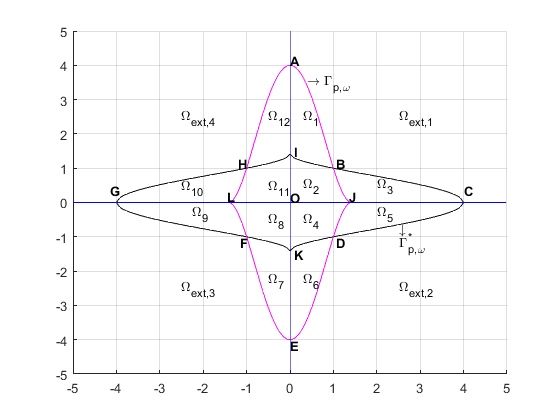
Figure 1: Partition of the plane $\mathbb{R}^{2}$ according to the curves $\Gamma_{p,\omega}$ and $\Gamma^{*}_{p,\omega}$ for $p=1.25$ and $\omega=2$.

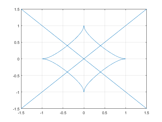
Figure 2: Partition of the plane $\mathbb{R}^{2}$ according to the curve $\Lambda_{p}$ (in blue) for $p=1.5$.

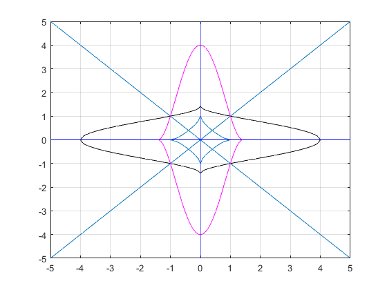
Figure 3: Partition of the plane $\mathbb{R}^{2}$ according to $\Lambda_{p,\omega}$, $\Gamma^{*}_{p,\omega}$ and $\Lambda_{p}$ for $p=1.5$ and $\omega=2$.

We now start developing our main results. For this aim, we assume in the rest of the paper that

$$\omega\geq 1\;\;\hbox{and}\;\;1<p<3.$$ (22)

It is straightforward that $\omega_{p}>\omega_{3}$. Moreover, the closed curves $\Gamma_{p,\omega}$ and $\Gamma^{*}_{p,\omega}$ intersect at four points $B$, $D$, $F$ and $H$ as it is shown in Figure 1. Notice also that the curves $\Gamma_{p,\omega}$ and $\Gamma^{*}_{p,\omega}$ split the plane $(u,v)$ into twelve regions, $\Omega_{i}$, $i=1,2,...,12$ and an external region $\Omega_{ext}=\displaystyle\bigcup_{1\leq i\leq 4}\Omega_{ext,i}$. Such regions are in the heart of the classification of solutions of problem (19)-(21). Notice also from the symmetry of the function $g_{\omega}$ that the points $B$ and $F$ satisfy the cartezian equation $u=v$ and the points $D$ and $H$ satisfy $u=-v$. Furthermore the polygon $BDFH$ is a square.

This symmetry also shows easily that whenever $(u,v)$ is a pair of solutions of the system (19), the pairs $(-u,v)$, $(u,-v)$ and $(-u,-v)$ are also solutions. Consequently, in the rest of the paper we will focus only on the case where $u(0)=a\geq 0$ and $v(0)=b\geq 0$. The remaining cases will be deduced by symmetry. As the function $f(u,v)$ is Locally Lipshitz continues, the existence and uniqueness of the solution is guaranteed by means of the famous Cauchy-Lipschitz theory. This will be recalled in the Appendix later.

Theorem 2.1

Whenever the initial data $(u(0),v(0))=(a,b)\in\Omega_{1}$, the problem (19)-(21) has a unique positive solution lieing in the same region $\Omega_{1}$. Furthermore,

i.

$u$ is nondecreasing,

ii.

$v$ is nonincreasing,

iii.

$(u,v)$ tends to $B$ as $x$ tends to $\infty$.

Proof. Writing problem (18) at $x=0$, yields that

$$u^{\prime\prime}(0)=-g_{\omega}(a,b)a>0\qquad\mbox{and}\qquad v^{\prime\prime}(0)=-g_{\omega}(b,a)b<0.$$

Hence, there exists $\delta>0$ small enought such that

$$u^{\prime\prime}(x)>0\qquad\mbox{and}\qquad v^{\prime\prime}(x)<0,\;\;\forall x\in(-\delta,\delta).$$

Consequently, $u^{\prime}$ is nondecreasing on $(-\delta,\delta)$ and $v^{\prime}$ is nonincreasing on $(-\delta,\delta)$. Next, as $u^{\prime}(0)=v^{\prime}(0)=0$, it therefore follows that $u$ is nonincreasing on $(-\delta,0)$ and nondecreasing on $(0,\delta)$ and that $v$ is nondecreasing on $(-\delta,0)$ and nonincreasing on $(0,\delta)$. Assume that $u$ remains nondeceasing on $(0,\infty)$. Then, we get at a first step $u(x)>a$, $\forall x>0$. Two situations may occur. $u$ has a finite limit $l_{u}$ which is obviously positive, or $u$ is going up to $\infty$ as $x$ goes up to $\infty$. Whenever the last situation occurs, we immediately get

$$u(x)\leq-x^{2}+K_{1}x+K_{2}$$

for some constants $K_{1}$ and $K_{2}$ and for $x$ large enough. Consequently, $u(x)\rightarrow-\infty$ as $x\rightarrow+\infty$. Which is a contradiction. Now, if the first case occurs, then, we immediately get a limit $L_{v}\geq 0$ of $v^{2}(x)$ as $x$ goes up to $\infty$. Thus, denoting $l_{v}=\sqrt{L_{v}}$, we get

$$g_{\omega}(l_{u},l_{v})=g_{\omega}(l_{v},l_{u})=0.$$

We claim that $(l_{u},l_{v})=B$. Indeed, if not, this means that the solution $(u,v)$ crosses one of the lines $(A,B)$ or $(B,I)$ at one point $X(x_{0})$. At $x_{0}$, we have

$$x_{0}>0,\;\;g_{\omega}(u(x_{0}),v(x_{0}))=0,\;\;g_{\omega}(v(x_{0}),u(x_{0}))>0.$$

Consider next the energy functional $E$ associated to problem (18) and defined by

$$E(u,v)(x)=\displaystyle\frac{1}{2}(u_{x}^{2}+v_{x}^{2})+\displaystyle\frac{1}{p+1}(|u|^{p+1}+|v|^{p+1})+\displaystyle\frac{\lambda}{2}u^{2}v^{2}-\displaystyle\frac{\omega}{2}(u^{2}+v^{2}).$$

It is straightforward that $E$ is constant as a function of $x$. Henceforth,

$$E(u,v)(x)=E(u,v)(0)=E(u,v)(\infty).$$

This equation may be written otherwise as

$$\frac{1}{p+1}(a^{p+1}+b^{p+1})+\displaystyle\frac{\lambda}{2}a^{2}b^{2}-\displaystyle\frac{\omega}{2}(a^{2}+b^{2})=\displaystyle\frac{2}{p+1}l^{p+1}+\displaystyle\frac{\lambda}{2}l^{4}-\omega l^{2},$$

where $l=l_{u}=|l_{v}|$ is the common limit of $u$ and $|v|$ at $\infty$. Denote next

$$H(u,v)=\displaystyle\frac{1}{p+1}(|u|^{p+1}+|v|^{p+1})+\displaystyle\frac{\lambda}{2}u^{2}v^{2}-\displaystyle\frac{\omega}{2}(u^{2}+v^{2}).$$

Whenever $u\in(a,u(x_{0}))$ and $v\in(v(x_{0}),b)$ or otherwise $x\in(0,x_{0})$, the functional $H$ is non-increasing as a function of $u$ and non-decreasing as a function of $v$. Hence forth,

$$E(u,v)(x_{0})<E(u,v)(x)<E(u,v)(0),$$

which is contradictory. As a consequence, we can state that $(u,v)$ does not cross the arc $(A,B)$. In addition, by similar techniques we can show that $(u,v)$ does not cross the arc $(I,B)$. So, necessarily, $(u,v)$ remains bounded in the domain $\Omega_{1}$. This yields that, $(u,v)$ tends to $B$ as $x$ tends to $\infty$.

Theorem 2.2

Whenever the initial data $(u(0),v(0))=(a,b)\in\Omega_{2}$, the problem (19)-(21) has a unique positive solution lieing in the same region $\Omega_{2}$. Furthermore,

i.

$u$ and $v$ are nondecreasing,

ii.

$(u,v)$ tends to $B$ as $x$ tends to $\infty$.

Proof. We proceed as in the proof of Theorem 2.1. At $x=0$, we have

$$u^{\prime\prime}(0)=-g_{\omega}(a,b)a>0\qquad\mbox{and}\qquad v^{\prime\prime}(0)=-g_{\omega}(b,a)b>0.$$

Therefore, as $u^{\prime}(0)=v^{\prime}(0)=0$, it follows that $u$ and $v$ are nondecreasing on $(0,\delta)$ for some $\delta>0$ small enough. Assume that $u$ remains nondecreasing on $(0,\infty)$. Then, we get at a first step $u(x)>a$, $\forall x>0$. Two situations may occur. $u$ has a finite limit $l_{u}$ which is obviously positive, or $u$ is going up to $\infty$ as $x$ goes up to $\infty$. Proceeding as in the proof of Theorem 2.1, we show that the second situation can not occur here also. So, assume that the second the first case occurs. Then, we immediately get a limit $L_{v}\geq 0$ of $v^{2}(x)$ as $x$ goes up to $\infty$. Denote as previously $l_{v}=\sqrt{L_{v}}$. Whenever $l_{v}=0$ (or equivalently $L_{v}=0$), then $l_{u}=\omega_{p}$. Consequently, $(u,v)\longrightarrow\,J$ as $x\longrightarrow+\infty$. Therefore the energy $E$ at $\infty$ becomes

$$E(l_{u},0)=l_{u}^{2}\omega\displaystyle\frac{1-p}{2(1+p)}>0.$$

On the other hand

$$E(u,v)(0)=\displaystyle\frac{a^{p+1}+b^{p+1}}{p+1}+\displaystyle\frac{\lambda}{20a^{2}b^{2}}-\displaystyle\frac{\omega}{2}(a^{2}+b^{2})>0.$$

So, we get a contradiction. Hence, $v$ is bounded but does not tend to 0 at $\infty$. Consequently, as $v^{2}$ has a limit $L_{v}$ at $\infty$, its derivative tends to 0 at $\infty$. So, necessarily $v^{\prime}$ and consequently $v^{\prime\prime}$ tend to 0 at $\infty$. The second equation of problem (18) yields then that $g_{\omega}(l_{v},l_{u})=0$. On $\partial\Omega_{2}$ it remains only the point $B$ to be the candidate for $(l_{v},l_{u})$.
Assume now that $u$ is not monotone on $(0,\infty)$ and let $x_{0}$ be its the first positive critical point. We get

$$E(u,v)(x_{0})>\displaystyle\frac{u(x_{0})^{p+1}+v(x_{0})^{p+1}}{p+1}+\displaystyle\frac{\lambda}{2}u(x_{0})^{2}v(x_{0})^{2}-\displaystyle\frac{\omega}{2}(u(x_{0})^{2}+v(x_{0})^{2})>0.$$

Whenever $(u(x_{0}),v(x_{0}))\in\Omega_{2}$, this leads to

$$E(u,v)(x_{0})>E(u,v)(0).$$

Which is contradictory. Next, whenever $(u(x_{0}),v(x_{0}))\notin\Omega_{2}$, consider the point $x_{1}$ to be the point at which $(u,v)$ crosses $\partial\Omega_{2}$. Three positions may hold. $(u(x_{1}),v(x_{1}))\in(B,J)$ or $(u(x_{1}),v(x_{1}))\in(I,B)$ or $(u(x_{1}),v(x_{1}))=B$. The last one leads to a stationary solution $(u,v)=B$. In the first case, we get again

$$E(u,v)(x_{1})>E(u,v)(0),$$

which is a contradiction (Similarly, for the second case). So, to conclude, we have proved that $(u,v)$ does not cross $\overline{\Omega_{2}}$. Thus the unique attractive point is $B$.

Now, similarly to the previous cases, we may prove the following result.

Theorem 2.3

Whenever the initial data $(u(0),v(0))=(a,b)\in\Omega_{3}$, the problem (19)-(21) has a unique positive solution lieing in the same region $\Omega_{3}$. Furthermore,

i.

$u$ is nonincreasing,

ii.

$v$ is nondecreasing,

iii.

$(u,v)$ tends to $B$ as $x$ tends to $\infty$.

We now study the case when the initial value is out of the negative zones of $g_{\omega}(u,v)$ and $g_{\omega}(v,u)$. We have the following result.

Theorem 2.4

Whenever the initial data $(u(0),v(0))=(a,b)\in\Omega_{ext}$, the problem (19)-(21) has a unique solution. Furthermore, $u$ and $v$ are not simultaneously monotone and satisfy

$$\lim_{x\rightarrow\infty}(u,v)(x)\in\Gamma^{\omega}_{p,\lambda}\cap\Gamma^{\omega,*}_{p,\lambda}.$$

Proof. We will prove the theorem for the case $(a,b)\in\Omega_{ext,1}$. The remaining ones may be proved by applying similar techniques. The starting point is always the same. We evaluate the behaviour of the solution at the origin $x=0$. We have

$$u^{\prime\prime}(0)=-g_{\omega}(a,b)a<0\qquad\mbox{and}\qquad v^{\prime\prime}(0)=-g_{\omega}(b,a)b<0.$$

Hence, as $u^{\prime}(0)=v^{\prime}(0)=0$, $u$ and $v$ are nonincreasing on $(0,\delta)$ for some $\delta>0$ small enough. Assume that $u$ remains nonincreasing on $(0,\infty)$. Two situations may occur. $u$ has a finite limit $l_{u}$, or $u$ is going down to $-\infty$ as $x$ goes up to $\infty$. Proceeding as in the proof of Theorem 2.1, we show that the second situation can not occur here-also. So, assume that the first case occurs. Then, we immediately get a limit $L_{v}\geq 0$ of $v^{2}(x)$ as $x$ goes up to $\infty$. Denote as previously $l_{v}=\sqrt{L_{v}}$. It is straightforward that $g_{\omega}(l_{u},l_{v})l_{u}=0$. We claim next that $g_{\omega}(l_{v},l_{u})=0$, Indeed, if it is not, we get

$$v^{\prime\prime}(x)\simeq-g_{\omega}(l_{v},l_{u})v\,;\,\,x\rightarrow\infty.$$

This means that

$$v(x)=K_{1}\cos(\omega x+\varphi)\,;\,\,x\rightarrow\infty$$

or

$$v(x)=K_{1}e^{-\omega x}+K_{2}e^{\omega x}\,;\,\,x\rightarrow\infty,$$

for some real constants $K_{1}$, $K_{2}$ and $\omega>0$. In the first case, $v^{2}$ does not have a limit as $x\rightarrow\infty$, except that $K_{1}=0$ and thus $v\equiv 0$ for $x$ large enough. In the second case, we get firstly $K_{2}=0$ for the same reason on $v^{2}$. Therefore, $v(x)\rightarrow 0$ as $x\rightarrow\infty$. So that, $l_{u}=0$ also. Which is contradictory. So now, we have obviously, $l_{u}=0$ or $l_{u}\neq 0$. Whenever the latter occurs we get $g_{\omega}(l_{u},l_{v})=g_{\omega}(l_{v},l_{u})=0$ and $l_{u}l_{v}\neq 0$. Which means that $(l_{u},l_{v})=\Gamma^{\omega}_{p,\lambda}\cap\Gamma_{p,\lambda}^{\omega,*}$. So we get furthemore $l_{u}=l_{v}=l$, where

$$l^{p-1}+\lambda l^{2}-w=0.$$

Now, applying the energy functional $E(u,v)$ and $H(u,v)$ we get

$$\frac{\partial H}{\partial u}=|u|^{p}+\lambda uv^{2}-wu=u(|u|^{p-1})+\lambda v^{2}-w=uf(u,v)>0$$

and

$$\frac{\partial H}{\partial v}=|v|^{p}+\lambda u^{2}v-wu=u(|u|^{p-1})+\lambda v^{2}-w=vf(v,u)>0.$$

Consequently,

$$H(u,v)(0)=E(u,v)(0)<H(u,v)(\infty)=E(u,v)(\infty)$$

which is contradictory. Consequently, one of the following situations hold.

• $u\searrow$, $v\searrow$, $(u,v)\longrightarrow B$ and $u\geq x_{B}$, $v\geq y_{B}$.

• $u$ and $v$ are not monotone on the whole interval $(0,\infty)$ and thus $(u,v)$ crosses the boundary $\partial\Omega^{c}_{ext}$ to $\Omega_{1}$ or $\Omega_{2}$ and thus $(u,v)$ is attracted by $B$ again.

Now, we will study the case $\ell_{u}=0$. We get in this case

$$v^{\prime\prime}+(|v|^{p-1}+\lambda u^{2})v=0.$$

At $\infty$ we obtain

$$v^{\prime\prime}+|v|^{p-1}v=0.$$

$v$ is $\searrow$ on $(0,\infty)$ for $\delta>0$ small enough. If it remains $\searrow$ on $(0,\infty$), it has a limit $l_{v}$ as $x\longrightarrow+\infty$. Whenever $l_{v}=-\infty$ we get for $x\longrightarrow+\infty$,

$$v(x)\geq x^{2}+k_{1}x+k_{2},$$

for some constants $k_{1},k_{2}$, which is contradictory. Whenever $l_{v}$ is finite and nonzero, we get at infinity

$$v(x)=k\cos(\delta x+\varphi)$$

which has no limit as $x\longrightarrow+\infty$. Consequently, $v$ can not be $\searrow$ on $(0,\infty)$. It remains that $u\searrow 0$ and $v\searrow 0$. This way, $(u,v)$ crosses $\Omega_{ext}$ to $\Omega_{int}$. Thus $(u,v)$ will be attracted by $B$ which contradicts the monotonicity.

We conclude thus that $u$ and $v$ can not be monotone simultaneously and that $(u,v)$ tends to one of the points $B,D,F,H$ of $\Gamma^{\omega}_{p,\lambda}\cap\Gamma_{p,\lambda}^{\omega,*}$.

We now study the case when the initial value lies on one of the curves $\Gamma_{p,\lambda}^{\omega}\cup\Gamma^{\omega,*}_{p,\lambda}$. Of course, whenever the initial value $(u(0),v(0))\in\Gamma_{p,\lambda}^{\omega}\cap\Gamma^{\omega,*}_{p,\lambda}$, the pair solution $(u,v)$ remains constant due to Cauchy-Lipschitz theorem. The interesting cases will be those when the initial value is on the graph $\Gamma_{p,\lambda}^{\omega}\cup\Gamma^{\omega,*}_{p,\lambda}\setminus\{B,D,F,H\}$. It holds in fact that the remaining vertices of the graph necessitates to be treated case by case. For this aim and throughout the remaining parts of the present paper, we denote $G$ the graph $\Gamma_{p,\lambda}^{\omega}\cup\Gamma^{\omega,*}_{p,\lambda}$ and $G^{\star}$ the graph $G$ without vertices. The following result is obtained.

Theorem 2.5

Whenever the initial data $(u(0),v(0))=(a,b)\in G^{\star}$, the problem (19)-(21) has a unique solution. Furthermore, $u$ and $v$ are not simultaneously monotone and satisfy

$$\lim_{x\rightarrow\infty}(u,v)(x)\in\Gamma_{p,\lambda}^{\omega}\cap\Gamma_{p,\lambda}^{\omega,\star}.$$

Proof. At the origin $x=0$, we get

$$u^{\prime\prime}(0)=u^{\prime}(0)=-g_{\omega}(a,b)a=0\qquad\mbox{and}\qquad v^{\prime\prime}(0)=-g_{\omega}(b,a)b<0.$$

We claim that $u$ can not remain constant on any interval $(0,\delta)$, $\delta>0$. Indeed, if this occurs on some interval $(0,\delta)$, we get immediately

$$u(x)=a\quad\mbox{and}\quad\lambda v^{2}(x)=\omega-a^{p-1}\,,\;\;\forall\,x\in(0,\delta).$$

So, $|v|$ is also constant ($\equiv b$) on $(0,\delta)$. Therefore, we get

$$v^{\prime\prime}+g_{\omega}(b,a)v=0\;\;\mbox{on}\;\;(0,\delta).$$

This means that

$$v(x)=K_{1}\cos(\rho x+\rho)\,;\,\,x\in(0,\delta),$$

which contradicts the fact that $|v|$ is constant, except if $K_{1}=0$. However, in this case we again get $b=0$, which is contradictory. So as the claim. Consequently, three situations may occur. $(i)$ the pair solution $(u,v)$ remains on the edge $)A,B($ and being non constant. $(ii)$ the pair solution $(u,v)$ bifurcates upward $\Omega_{ext,1}$. $(iii)$ the pair solution $(u,v)$ bifurcates toward $\Omega_{1}$. The case (i): $(u,v)$ remains on $)A,B($. We get $u(x)=a,\forall x\in(0,\infty)$ which is a contradictory with the previous claim. Assume now that the situation (ii) or (iii) occur. Thus it is attracted by the limit point $B$.

Next, observing that the nonlinear function $f(u,v)=(|u|^{p-1}+\lambda|v|^{2})u$ has some parity characteristics relatively to $u$ and $v$, the analogous of Theorems 2.1, 2.2, 2.3, 2.4, 2.5 may be obtained. We precisely get

Theorem 2.6

Whenever the initial data $(u(0),v(0))=(a,b)\in\displaystyle\bigcup_{i=4}^{12}\Omega_{i}$, the problem (19)-(21) has a unique solution lieing in the same region $\Omega_{i}$ that contains its initial value $(a,b)$ . Furthermore,

1. For $(a,b)\in\Omega_{4}$,

   i.

   $u$ is positive and nonincreasing,

   ii.

   $v$ is negative and nondecreasing,

   iii.

   $(u,v)$ tends to $D$ as $x$ tends to $\infty$.

2. For $(a,b)\in\Omega_{5}$,

   i.

   $u$ is positive and nondecreasing,

   ii.

   $v$ is negative and nondecreasing,

   iii.

   $(u,v)$ tends to $D$ as $x$ tends to $\infty$.

3. For $(a,b)\in\Omega_{6}$,

   i.

   $u$ is positive and nondecreasing,

   ii.

   $v$ is negative and nondecreasing,

   iii.

   $(u,v)$ tends to $D$ as $x$ tends to $\infty$.

4. For $(a,b)\in\Omega_{7}$,

   i.

   $u$ is negative and nonincreasing,

   ii.

   $v$ is negative and nondecreasing,

   iii.

   $(u,v)$ tends to $F$ as $x$ tends to $\infty$.

5. For $(a,b)\in\Omega_{8}$,

   i.

   $u$ is negative and nonincreasing,

   ii.

   $v$ is negative and nonincreasing,

   iii.

   $(u,v)$ tends to $F$ as $x$ tends to $\infty$.

6. For $(a,b)\in\Omega_{9}$,

   i.

   $u$ is negative and nondecreasing,

   ii.

   $v$ is negative and nonincreasing,

   iii.

   $(u,v)$ tends to $F$ as $x$ tends to $\infty$.

7. For $(a,b)\in\Omega_{10}$,

   i.

   $u$ is negative and nondecreasing,

   ii.

   $v$ is positive and nondecreasing,

   iii.

   $(u,v)$ tends to $H$ as $x$ tends to $\infty$.

8. For $(a,b)\in\Omega_{11}$,

   i.

   $u$ is negative and nonincreasing,

   ii.

   $v$ is positive and nondecreasing,

   iii.

   $(u,v)$ tends to $H$ as $x$ tends to $\infty$.

9. For $(a,b)\in\Omega_{12}$,

   i.

   $u$ is negative and nonincreasing,

   ii.

   $v$ is positive and nonincreasing,

   iii.

   $(u,v)$ tends to $H$ as $x$ tends to $\infty$.

3 Conclusion

In [Yaping], a system of coupled NLS and Heat equations has been considered for exponential stability in a torus region. The basic idea consists of transforming the system into one-dimensional coupled one by applying polar coordinates.

Inspired from the present work, in forthcomming works, we intend to consider analogoue study with

• The Heat operator

  $$\mathcal{L}_{i}(u(x,t))=\mathcal{H}_{i}(u(x,t))=u_{t}-\sigma_{i}\Delta u$$

  leading to a nonlinear Heat system.

• The mixed Schrödinger-Heat operator

  $$\mathcal{L}(u(,v))=(\mathcal{L}_{1}(u),\mathcal{L}_{2}(v))=(\mathcal{S}(u),\mathcal{H}(v))$$

  leading to a nonlinear coupled system of Schrödinger-Heat type.

4 Appendix

4.1 Appendix A

Recall that in the previous sections, we applied for many times the well-known Cauchy Lipschitz theorem on the existence and uniqueness of solutions. In this section and for convenience, we will show that the generator function used is already locally Lipschitz continuous.

Denote $\varphi=u^{\prime}$ and $\psi=v^{\prime}$. The system (19)-(21) becomes

$$\left\{\begin{array}[]{lll}u^{\prime}=\varphi\\ \varphi^{\prime}=-(|u|^{p-1}+|v|^{2})u,\\ v^{\prime}=\psi\\ \psi^{\prime}=-(|v|^{p-1}+|u|^{2})v,\\ u(0)=a,\;v(0)=b,\;\varphi(0)=0,\;\psi(0)=0.\end{array}\right.$$ (23)

Denoting $X$ the vector $X=(u,v,\varphi,\psi)^{T}$, where ^T stands for the transpose, we get

$$X^{\prime}=F(X),\;X(0)=(a,b,0,0)^{T},$$

where $F$ is the function defined by

$$F(x_{1},x_{2},x_{3},x_{4})=(x_{2},-g_{\omega}(x_{1},x_{3})x_{1},x_{4},-g_{\omega}(x_{3},x_{1})x_{3}),\;\;(x_{1},x_{2},x_{3},x_{4})\in\mathbb{R}^{4}.$$

Lemma 4.1

$F$ is locally Lipschitz continuous on $\mathbb{R}^{4}$.

Proof. Let $\delta>0$ small enough and $X^{0}=(x_{1}^{0},x_{2}^{0},x_{3}^{0},x_{4}^{0})\in\mathbb{R}^{4}$ be fixed. For all $X,Y$ in the ball $B(X^{0},\delta)$ we have

$$\begin{array}[]{lll}\|F(X)-F(Y)\|_{2}^{2}&=&(x_{2}-y_{2})^{2}+(x_{4}-y_{4})^{2}\\ &&+(g(x_{1},x_{3})x_{1}-g(y_{1},y_{3})y_{1})^{2}\\ &&+(g(x_{3},x_{1})x_{3}-g(y_{3},y_{1})y_{3})^{2}.\end{array}$$

We shall now evaluate the quantity $(g(x_{1},x_{3})x_{1}-g(y_{1},y_{3})y_{1})^{2}$. Similar techniques will lead to $(g(x_{3},x_{1})x_{3}-g(y_{3},y_{1})y_{3})^{2}$. We have

$$\begin{array}[]{lll}&&|g(x_{1},x_{3})x_{1}-g(y_{1},y_{3})y_{1})|\\ &=&||x_{1}|^{p-1}x_{1}-|y_{1}|^{p-1}y_{1}+\lambda(|x_{3}|^{2}x_{1}-|y_{3}|^{2}y_{1})|\\ &\leq&||x_{1}|^{p-1}x_{1}-|y_{1}|^{p-1}y_{1}|+\lambda||x_{3}|^{2}x_{1}-|y_{3}|^{2}y_{1}|\\ &\leq&C_{1}(p,X_{0},\delta)|x_{1}-y_{1}|+\lambda\left[||x_{3}|^{2}-|y_{3}|^{2}||x_{1}|+|x_{1}-y_{1}||y_{3}|^{2}\right]\\ &\leq&C_{1}(p,X_{0},\delta)|x_{1}-y_{1}|+\lambda C_{2}(X_{0},\delta)\left[||x_{3}-y_{3}|+|x_{1}-y_{1}|\right]\\ &\leq&C_{1}(p,X_{0},\delta)|x_{1}-y_{1}|+\lambda C_{2}(X_{0},\delta)\left[||x_{3}-y_{3}|+|x_{1}-y_{1}|\right]\\ &\leq&C(p,X_{0},\delta,\lambda)\left[||x_{3}-y_{3}|+|x_{1}-y_{1}|\right],\end{array}$$

where $C_{1}(p,X_{0},\delta)>0$ is a constant depending only on $p$, $X_{0}$ and $\delta$. $C_{2}(X_{0},\delta)>0$ is a constant depending only on $X_{0}$ and $\delta$. $C(p,X_{0},\delta,\lambda)>0$ is a constant depending only on $p$, $X_{0}$, $\delta$ and $\lambda$. Therefore,

$$\begin{array}[]{lll}|g(x_{1},x_{3})x_{1}-g(y_{1},y_{3})y_{1})|^{2}&\leq&C(p,X_{0},\delta,\lambda)^{2}\left[||x_{3}-y_{3}|+|x_{1}-y_{1}|\right]^{2}\\ &\leq&2C(p,X_{0},\delta,\lambda)^{2}\left[||x_{3}-y_{3}|^{2}+|x_{1}-y_{1}|^{2}\right].\end{array}$$

Similarly,

$$|g(x_{3},x_{1})x_{3}-g(y_{3},y_{1})y_{3})|^{2}\leq 2\widetilde{C}(p,X_{0},\delta,\lambda)^{2}\left[||x_{3}-y_{3}|^{2}+|x_{1}-y_{1}|^{2}\right],$$

with some constant $\widetilde{C}(p,X_{0},\delta,\lambda)>0$ analogue to ${C}(p,X_{0},\delta,\lambda)$. Combining all these inequalities, we obtain

$$\|F(X)-F(Y)\|_{2}^{2}\leq C(p,X_{0},\delta,\lambda)\|X-Y\|_{2}^{2},\;\;\forall\,X,Y\in\,B(X_{0},\delta).$$

4.2 Appendix B

In this part, we investigate the dependence of the different regions and curves $\Omega_{i}$, $i=1,\dots,12$, $\Omega_{ext,i}$, $i=1,\dots,4$ and the different curves $\Gamma^{\omega}_{p,\lambda}$, $\Gamma^{\omega,*}_{p,\lambda}$ and $\Lambda_{p}$. So denote $\Lambda_{p}^{*}=\Lambda_{p}\setminus\{(u,v)\in\mathbb{R}^{2};\;|u|\not=|v|\}$. Denote also $\Omega_{int}=\displaystyle\bigcup_{i=1}^{12}\Omega_{i}$ and $\mathcal{A}_{p}$ the interior area countered by the curve $\Lambda_{p}^{*}$.

Lemma 4.2

The erea $\mathcal{A}_{p}\subset[-1,1]^{2}$.

Indde, denote for $(u,v)\in\mathcal{A}_{p}$

$$u=r\cos\theta,\;\;v=r\sin\theta.$$

It is staightforward that $r$ is maximum whenever $(u,v)$ is on the frontier $\Lambda_{p}^{*}$, which may be then governed by the polar equation

$$r^{p-3}\biggl{(}|\cos\theta|^{p-1}-|\sin\theta|^{p-1}\biggr{)}=\cos(2\theta).$$

Otherwise,

$$r^{p-3}=\displaystyle\frac{\cos(2\theta)}{|\cos\theta|^{p-1}-|\sin\theta|^{p-1}}.$$

Straightforward calculus yield that whenever $0<p<3$, the radius $r$ is extremum for $\theta\in\{0,\pm\frac{\pi}{2},\pi\}$, which gives the vertices $(\pm 1,0)$, $(0,\pm 1)$. In fact $r(_{t}heta)$ may be extended at $\theta=\{\pm\frac{\pi}{4},\pm\frac{3\pi}{4}\}$. However, these points yield immediately $|u|=|v|$, which is the trivial (unbounded) part of $\Lambda_{p}$.

As a result of Lemma 4.2, we immediately deduce that whenever $0<\omega\leq 1$ and $1<p<3$ the inclusion $\Omega_{int}\subset\mathcal{A}_{p}$. However, for $\omega\geq 1$ and $1<p<3$, the area $\subset\mathcal{A}_{p}$ is contained in the curved octagonal shape $IBJDKFLH$.

Figure 4: Parameters’ domains for $p=1.5$, $\omega=0.5$

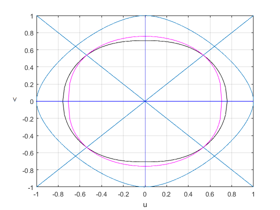
Figure 5: Parameters’ domains for $p=3.5$, $\omega=0.5$

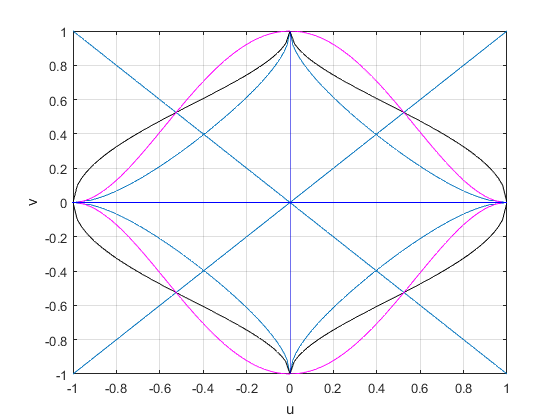
Figure 6: Parameters’ domains for $p=1.5$, $\omega=1$

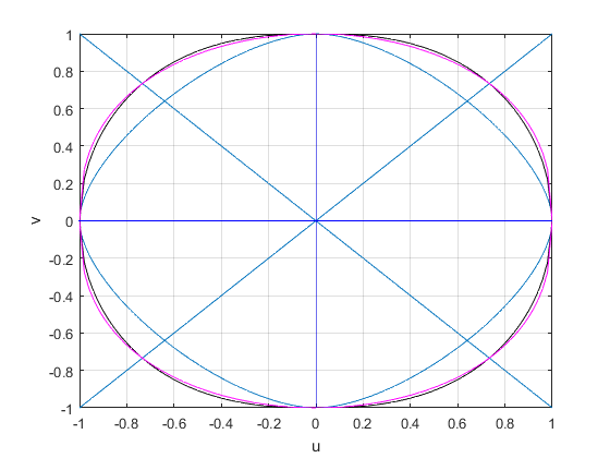
Figure 7: Parameters’ domains for $p=3.5$, $\omega=1$

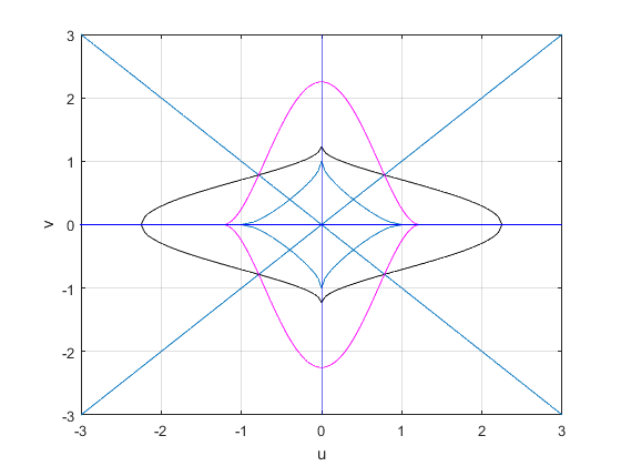
Figure 8: Parameters’ domains for $p=1.5$, $\omega=1.5$

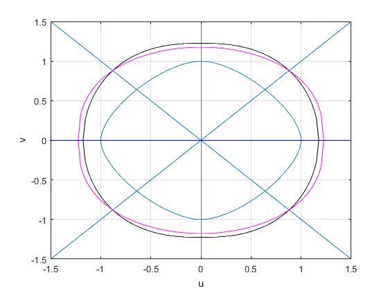
Figure 9: Parameters’ domains for $p=3.5$, $\omega=1.5$

References

- [1] J. S. Aitchison, A. M. Weiner, Y. Silberberg, D. E. Leaird, M. K. Oliver, J. L. Jackel and P. W. E. Smith, 1991 Opt. Lett.
- [2] H. Aminikhah, F. Pournasiri and F. Mehrdoust, C. Pramana, Journal of Physics, Indian Academy of Sciences. Vol. 86, No. 1, (2016), pp. 19–30.
- [3] A. Bahrouni, A Note on the Existence Results for Schrödinger-Maxwell System with Super-Critical Nonlinearitie. Acta Appl Math (2019). https://doi.org/10.1007/s10440-019-00263-3.
- [4] B. Balabane, J. Dolbeault and H. Ounaeis, Nodal solutions for a sublinear elliptic equation, Nonlinear analysis, 52 (2003), 219-237.
- [5] A. M. Batista and M.F. Furtado, Positive and nodal solutions for a nonlinear Schrödinger-Piosson system with sign-changing potentials, Nonlinear Anal. Real World Appl. 39 (2018), 142-156.
- [6] V. Benci and D. F. Fortunato, Solitary waves of the nonlinear Klein-Gordon equation coupled with Maxwell equations. Reviews in Mathematical PhysicsVol. 14, No. 04, pp. 409-420 (2002).
- [7] R. D. Benguria, J. Dolbeault and M. J. Esteban, Classification of the solutions of semilinear elliptic problems in a ball. J. Diff. Eq. 167 (2000), 438-466.
- [8] A. Ben Mabrouk and M. Ayadi, A linearized finite-difference method for the solution of some mixed concave and convex nonlinear problems. Applied Mathematics and Computation. 197(1) (2008), 1-10.
- [9] A. Ben Mabrouk and M Ayadi, Lyapunov type operators for numerical solutions of PDEs. Appl. Math. and Computa., 204(1) (2008), 395-407.
- [10] A. Ben Mabrouk and M. L. Ben Mohamed, Nodal solutions for some nonlinear elliptic equations. Applied Mathematics and Computation. 186(1) (2007), 589-597.
- [11] A. Ben Mabrouk and M. L. Ben Mohamed, Phase plane analysis and classification of solutions of a mixed sublinear-superlinear elliptic problem. Nonlinear Analysis: Theory, Methods & Applications, 70(1) (2009), 1-15.
- [12] A. Ben Mabrouk and M. L. Ben Mohamed, Nonradial solutions of a mixed concave-convex elliptic problem. J. Part. Diff. Eq., 24(4) (2011), 313-323.
- [13] A. Ben Mabrouk and M. L. Ben Mohamed, On some critical and slightly super-critical sub-superlinear equations. Far East J. Appl. Math. 23(1) (2006), 73-90.
- [14] A. Ben Mabrouk, M. L. Ben Mohamed and K. Omrani, Finite difference approximate solutions for a mixed sub-superlinear equation. Applied Mathematics and Computation. 187(2) (2007), 1007-1016.
- [15] R. Chteoui, A. Ben Mabrouk and H. Ounaies, Existence and Properties of Radial Solutions of a Sublinear Elliptic Equation, J. Part. Diff. Eq., 28(1) (2015), 1-9.
- [16] R. Chteoui, A. F. Aljohani and A. Ben Mabrouk, On a mixed cubic-superlinear Schrödinger systems, Part I: Existence and uniqueness of steady state solutions. Submitted.
- [17] R. Chteoui, A. F. Aljohani and A. Ben Mabrouk, On a mixed cubic-superlinear Schrödinger system, Part II: Lyapunov-Sylvester computational method for Numerical Solutions. Submitted.
- [18] K. Chaib, Necessary and sufficient conditions of existence for a system involving the -Laplacian . J. Differential Equations 189 (2003) 513-525.
- [19] S. Chakravarty, M. J. Ablowitz, J. R. Sauer and R. B. Jenkins, Multisoliton interactions and wavelength-division multiplexing. Opt. Lett. 20(2) (1995), 136-138.
- [20] A. K. Dhar and K. P. Das, Fourth-order nonlinear evolution equation for two Stokes wave trains in deep water. Physics of Fluids A: Fluid Dynamics 3, 3021 (1991).
- [21] M. R. Gupta, B. K. Som, B. Dasgupta, Coupled nonlinear Schrödinger equations for Langmuir and elecromagnetic waves and extension of their modulational instability domain. J. Plas, Phys. 25(3) (1981) pp. 499-507.
- [22] F. T. Hioe, Solitary waves for two and three coupled nonlinear Schrödinger equations. Phys. Rev. E 58 (1998) 6700.
- [23] T. Kanna, M. Lakshmanan, P. T. Dinda and N. Akhmediev, Soliton collisions with shape change by intensity redistribution in mixed coupled nonlinear Schrödinger equations. Phys. Rev. E 73 (2006), 026604.
- [24] C. E. Kenig and F. Merle, Global well-posedness, scattering and blow-up for the energy-critical, focusing, non-linear Schrödinger equation in the radial case. Invent. Math. 166 (2006), 645-675.
- [25] S. Keraani, On the blow-up phenomenon of the critical Schrödinger equation. J. Funct. Anal. 235 (2006), 171-192.
- [26] H. Liu, Ground states of linearly coupled Schrödinger systems, Electronic Journal of Differential Equations, Vol. 2017 (2017), No. 05, pp. 1–10.
- [27] Y. Martel and F. Merle, Multi solitary waves for nonlinear Schrödinger equations. Ann. I. H. poincaré. 23 (2006), 849-864.
- [28] C. R. Menyuk, Stability of solitons in birefringent optical fibers. II. Arbitrary amplitudes. Journal of the Optical Society of America B Vol. 5, Issue 2, (1988), pp. 392-402.
- [29] F. Merle, Construction of solutions with exactly blow-up points for the Schrödinger equation with critical nonlinearities. Comm. Math. Phys. 129 (1990), 223-240.
- [30] L. F. Mollenauer, S. G. Evangelides and J. P. Gordon, Wavelength division multiplexing with solitons in ultra-long distance transmission using lumped amplifiers. J. Lightwave Technol. 9 (1991), 362
- [31] H. Ounaies, Study of an elliptic equation with a singular potential, Indian J. Pure appl. Math., 34(1) (2003), 111-131.
- [32] C. V. Pao, Nonlinear parabolic and elliptic equations, Plenum Press, New York, 1992.
- [33] Z. Pinar and E. Deliktas, Solution behaviors in coupled Schrödinger equations with full-modulated nonlinearities. AIP Conference Proceedings 1815, 080019 (2017).
- [34] L. Ping and S. Y. Lou, Coupled Nonlinear Schrödinger Equation: Symmetries and Exact Solutions. Communications in Theoretical Physics 51(1) (2009), pp. 27-34.
- [35] A. Quaas, B. Sirakov, Existence and non-existence results for fully nonlinear elliptic systems. Indiana University Mathematics Journal, 58 (2) (2009), pp. 751-788.
- [36] S. H. Rasouli, M. Choubin, The Nehari manifold approach for a class of nonlinear elliptic systems. Monatshefte für Mathematik, 2014, 173, 4, pp. 605-623.
- [37] T. Saanouni, A note on coupled focusing nonlinear Schrödinger equations. J, Applicable Analysis, An International Journal, Volume 95(9), (2016) pp. 2063-2080
- [38] J. Serrin and H. Zou, Classification of positive solutions of quasilinear elliptic equations. Topol. Methods Nonlinear Anal., 3 (1994), 1-26.
- [39] M. Shalaby, F. Reynaud and A. Barthelemy, Experimental observation of spatial soliton interactions with a relative phase difference. Opt. Lett. 17(11) (1992), pp. 778-780.
- [40] W. A. Strauss, Existence of Solitary Waves in Higher Dimensions. Commun. math. Phys. (1977), 149—162.
- [41] S. L. Yadava, Uniqueness of positive radial solutions of the Dirichlet problems in an annulus. J. Diff. Eq., 139 (1997), 194-217.
- [42] E. Yanagida, Structure of radial solutions to in . SIAM. J. Math. Anal., 27 (1996), 997-1014.
- [43] H.-Q. Zhang, X.-H. Meng, T. Xu, L.-L. Li and B. Tian, Interactions of bright solitons for the (2+1)-dimensional coupled nonlinear Schrödinger equations from optical fibres with symbolic computation. Physica Scripta 75(4) (2007) pp. 537-542.
- [44] Y. Zhida, Multi-soliton solutions of coupled nonlinear Schrödinger Equations. J Chinese Physics Letters 4(4) (1987) pp. 185-187.
- [45] S. Zhou, X. Cheng, Numerical solution to coupled nonlinear Schrödinger equations on unbounded domains. Mathematics and Computers in Simulation 80(12), (2010), pp. 2362-2373.