Double-heavy axial-vector tetraquark $T_{bc;\bar{u}\bar{d}}^{0}$

Abstract

The mass and coupling of the axial-vector tetraquark $T_{bc;\bar{u}\bar{d}}^{0}$ (in a short form $T_{bc}^{0}$) are calculated by means of the QCD two-point sum rule method. In computations we take into account contributions arising from various quark, gluon and mixed vacuum condensates up to dimension 10. The central value of the mass $m=(7105\pm 155)~{}\mathrm{MeV}$ lies below the thresholds for the strong and electromagnetic decays of $T_{bc}^{0}$ state, and hence it transforms to conventional mesons only through the weak decays. In the case of $m=7260~{}\mathrm{MeV}$ the tetraquark $T_{bc}^{0}$ becomes the strong- and electromagnetic-interaction unstable particle. In the first case, we find the full width and mean lifetime of $T_{bc}^{0}$ using its dominant semileptonic decays $T_{bc}^{0}\to T_{cc;\bar{u}\bar{d}}^{+}l\overline{\nu}_{l}$ ($l=e,\ \mu,\tau$), where the final-state tetraquark is a scalar state. We compute also partial widths of the nonleptonic weak decays $T_{bc}^{0}\to T_{cc;\bar{u}\bar{d}}^{+}\pi^{-}(K^{-},D^{-},D_{s}^{-})$, and take into account their effects on the full width of $T_{bc}^{0}$. In the context of the second scenario we calculate partial widths of $S$-wave strong decays $T_{bc}^{0}\to B^{\ast-}D^{+}$ and $T_{bc}^{0}\to\overline{B}^{\ast 0}D^{0}$, and using these channels evaluate the full width of $T_{bc}^{0}$. Predictions for $\Gamma_{\mathrm{full}}=(3.98\pm 0.51)\times 10^{-10}~{}\mathrm{MeV}$ and mean lifetime $\tau=1.65_{-0.18}^{+0.25}~{}\mathrm{ps}$ of $T_{bc}^{0}$ obtained in the context of the first option, as well as the full width $\Gamma_{\mathrm{full}}=(63.5\pm 8.9)~{}\mathrm{MeV}$ extracted in the second scenario may be useful for experimental and theoretical exploration of double-heavy exotic mesons.

I Introduction

During last two decades double-heavy tetraquarks as real candidates for stable four-quark states became subjects of intensive studies. In the pioneering papers Ader:1981db ; Lipkin:1986dw ; Zouzou:1986qh it was demonstrated that a heavy $Q$ and light $q$ quarks may form the stable exotic mesons $QQ\bar{q}\bar{q}$ provided the ratio $m_{Q}/m_{q}$ is large enough. These results were obtained in the context of a potential model with the additive pairwise interaction, but even models with relaxed restrictions on the confining potential led to the similar predictions. Indeed, in accordance with Ref. Carlson:1987hh the isoscalar axial-vector tetraquark $T_{bb;\overline{u}\overline{d}}^{-}$ turns to be strong-interaction stable state that lies below the $B\overline{B}^{\ast}$ threshold. It is worth noting that an only constraint imposed in Ref. Carlson:1987hh on the potential was its finiteness at close distances of two particles. Therefore, $T_{bb;\overline{u}\overline{d}}^{-}$ decays to conventional mesons only through weak processes and has a long lifetime, which is important for its experimental exploration. A situation with the tetraquarks $T_{bc;\bar{q}\bar{q}^{\prime}}$ and $T_{cc;\bar{q}\bar{q}^{\prime}}$ was not clear, because $bc$ and $cc$ diquarks might constitute both stable and unstable states.

In years followed after this progress, various models of high energy physics were used to investigate the double-heavy tetraquarks $T_{QQ}$ Janc:2004qn ; Cui:2006mp ; Vijande:2006jf ; Ebert:2007rn ; Navarra:2007yw ; Du:2012wp ; Hyodo:2012pm ; Esposito:2013fma . Recent interest to these problems was inspired by results of the LHCb Collaboration on properties of the doubly charmed baryon $\Xi_{cc}^{++}=ccu$ Aaij:2017ueg . Parameters of this baryon were used in Ref. Karliner:2017qjm to evaluate the mass and analyze possible decay channels of $T_{bb;\overline{u}\overline{d}}^{-}$. Predictions obtained there confirmed the stability of $T_{bb;\overline{u}\overline{d}}^{-}$ against the strong and electromagnetic decays to $B^{-}\overline{B}^{\ast 0}$ and $B^{-}\overline{B}^{0}\gamma$, respectively. The strong-interaction stable nature of the tetraquarks $T_{bb;\overline{u}\overline{d}}^{-}$, $T_{bb;\overline{u}\overline{s}}^{-}$, and $T_{bb;\overline{d}\overline{s}}^{0}$ was demonstrated in Ref. Eichten:2017ffp by invoking heavy-quark symmetry relations. The mass and coupling of $T_{bb;\overline{u}\overline{d}}^{-}$ was evaluated in our work Agaev:2018khe as well, in which we estimated also its full width and mean lifetime using the semileptonic decay channel $T_{bb;\overline{u}\overline{d}}^{-}\rightarrow Z_{bc;\overline{u}\overline{d}}^{0}l\bar{\nu_{l}}$ .

Another class of four-quark mesons, namely one that contains the heavy diquarks $bc$ is on agenda of physicists as well. The scalar and axial-vector tetraquarks $bc\overline{u}\overline{d}$ are particles of special interest, because they may form strong-interaction stable compounds. But calculations performed in the context of different approaches lead controversial results. Thus, the Bethe-Salpeter method predicts the mass of the scalar tetraquark $Z_{bc;\overline{u}\overline{d}}^{0}$ (in what follows $Z_{bc}^{0}$) at around $6.93~{}\mathrm{GeV}$, which is below the threshold $7145~{}\mathrm{MeV}$ for $S$-wave strong decays to heavy mesons $B^{-}D^{+}$ and $\overline{B^{0}}D^{0}$ Feng:2013kea . Recent analysis demonstrated that $Z_{bc}^{0}$ lies $11~{}\mathrm{MeV}$ below this threshold Karliner:2017qjm , whereas the authors of Ref. Eichten:2017ffp found the masses of the scalar and axial-vector tetraquarks $bc\overline{u}\overline{d}$ equal to $7229~{}\mathrm{MeV}$ and $7272~{}\mathrm{MeV}$, respectively. These predictions make kinematically allowed their strong decays to ordinary $B^{-}D^{+}/\overline{B}^{0}D^{0}$ and $B^{\ast}D$ mesons.

It is interesting that lattice calculations prove the strong-interaction stabile nature of the axial-vector tetraquark $ud\overline{b}\overline{c}$, because its mass is below the $\overline{D}B^{\ast}$ threshold Francis:2018jyb . However, the authors could not decide would this exotic meson decay weakly or might transform also to the final state $\overline{D}B\gamma$. The stability of $J^{P}=0^{+}$ and $1^{+}$ isoscalar tetraquarks $bc\overline{u}\overline{d}$ was confirmed in Ref. Caramees:2018oue , in which it was found that $J^{P}=0^{+}$ state is a strong- and electromagnetic-interaction stable particle, whereas $J^{P}=1^{+}$ may also transform through the electromagnetic interaction.

In the context of the QCD sum rule approach the spectroscopic parameters of the scalar tetraquark $Z_{bc}^{0}$ were calculated also in our work Agaev:2018khe . For the mass of $Z_{bc}^{0}$ computations predicted $m_{Z}=(6660\pm 150)~{}\mathrm{MeV}$, which is considerably below the threshold $7145~{}\mathrm{MeV}$. The electromagnetic decay modes $Z_{bc}^{0}\rightarrow\overline{B}^{0}D_{1}^{0}\gamma$ and $B^{\ast}D_{0}^{\ast}\gamma$ are among forbidden processes as well, because relevant thresholds exceed $7600~{}\mathrm{MeV}$ and are higher than the mass of $Z_{bc}^{0}$. In other words, in accordance with our results the scalar tetraquark $Z_{bc}^{0}$ is a strong- and electromagnetic-interaction stable particle. The $Z_{bc}^{0}$ transforms due to weak decays, which allowed us to find in Ref. Sundu:2019feu its full width and mean lifetime.

In the present article we study the axial-vector tetraquark $T_{bc;\overline{u}\overline{d}}^{0}$ (hereafter $T_{bc}^{0}$) by computing its spectroscopic parameters, full width and mean lifetime. The mass $m$ and coupling $f$ of $T_{bc}^{0}$ are evaluated in the framework of the QCD two-point sum rule method by taking into account vacuum expectation values of the local quark, gluon and mixed operators up to dimension ten. The mass of $T_{bc}^{0}$ extracted in the present work $m=(7105\pm 155)~{}\mathrm{MeV}$ contains theoretical errors typical for sum rule computations, hence, there are two options to find its full width and estimate mean lifetime. Thus, the central value of the mass is lower than the thresholds $7190~{}\mathrm{MeV}$ and $7286~{}\mathrm{MeV}$ for strong $S$-wave decays of $T_{bc}^{0}$ to final states $B^{\ast-}D^{+}/\overline{B}^{\ast 0}D^{0}$ and $B^{-}D^{\ast+}/\overline{B}^{0}D^{\ast 0}$, respectively. This mass is also lower than the threshold $7145~{}\mathrm{MeV}$ for the electromagnetic decays $D^{+}B^{-}\gamma/D^{0}\overline{B}^{0}\gamma$. Therefore, in this case the full width and lifetime of the exotic meson $T_{bc}^{0}$ should be determined from its weak decays. But considering the maximum theoretical prediction for $m=7260$ $\mathrm{MeV}$, one sees that it is higher than the threshold for strong decays $B^{\ast-}D^{+}/\overline{B}^{\ast 0}D^{0}$ and electromagnetic transitions $D^{+}B^{-}\gamma/D^{0}\overline{B}^{0}\gamma$. Realization of this scenario means that the width of the tetraquark $T_{bc}^{0}$ is determined mainly by strong decays, because partial widths of weak and electromagnetic processes are very small and can be neglected.

Here, to calculate the full width of the tetraquark $T_{bc}^{0}$, we consider both scenarios. In the first case $m=7105~{}\mathrm{MeV}$, and the processes $T_{bc}^{0}\rightarrow T_{cc;\overline{u}\overline{d}}^{+}l\overline{\nu}_{l}$ ($l=e,\mu$ and $\tau$), where the final-state tetraquark $T_{cc;\overline{u}\overline{d}}^{+}$ (in what follows $T_{cc}^{+}$ ) is a scalar particle, are the dominant semileptonic decay channels of $T_{bc}^{0}$. These decays run due to transition $b\rightarrow W^{-}c$. The differential rates of these semileptonic decays are determined by the weak form factors $G_{i}(q^{2})$ ($i=0,1,2,3$), which are evaluated by employing the QCD three-point sum rule approach. Then, partial width of the processes $T_{bc}^{0}\rightarrow T_{cc}^{+}l\overline{\nu}_{l}$ can be found by integrating the relevant differential rates over the momentum transfer $q^{2}$. The sum rule method does not encompass all kinematically allowed values of $q^{2}$, therefore we introduce fit functions that coincide with sum rule predictions, and can be extrapolated to cover a whole integration region.

But a decay $b\rightarrow W^{-}c$ can be followed by transitions $W^{-}\rightarrow d\overline{u},\ s\overline{u},\ d\overline{c}$ and $s\overline{c}$ as well. Afterwards these quark pairs can form ordinary mesons through different mechanisms. Thus, in the hard-scattering picture a pair $d\overline{u}$ , for example, can create conventional mesons with $q\overline{q}$ quarks appeared due to a gluon from one of $d$ or $\overline{u}$ quarks. These processes generate final states $T_{bc}^{0}\rightarrow T_{cc}^{+}M_{1}(d\overline{q})M_{2}(q\overline{u})$ which are suppressed relative to the semileptonic decays by the factor $\alpha_{s}^{2}|V_{ud}|^{2}$. Alternatively, pairs of quarks $d\overline{u},\ s\overline{u},\ d\overline{c}$ and $s\overline{c}$ can form $\pi^{-}$, $K^{-\text{ }}$, $D^{-}$ and $D_{s}^{-}$ mesons triggering the two-body nonleptonic decays $T_{bc}^{0}\rightarrow T_{cc}^{+}\pi^{-}(K^{-\text{ }},D^{-},D_{s}^{-})$. Another class of the $T_{bc}^{0}$ tetraquark’s weak decays is connected with possibility of direct combination of these quarks with ones from $T_{cc;\overline{u}\overline{d}}^{+}$ and creation of three-meson final states. The two-body and three-meson nonleptonic decays do not suppressed by additional factors relative to the semileptonic decays, and their contributions to full width of $T_{bc}^{0}$ may be considerable.

In the second scenario $m=7260~{}\mathrm{MeV}$, and this mass is above the threshold for strong decays to mesons $B^{\ast-}D^{+}/\overline{B}^{\ast 0}D^{0}$, but is still below the threshold for other two possible decay modes to final states $B^{-}D^{\ast+}/\overline{B}^{0}D^{\ast 0}$. Therefore, we calculate the partial width of the kinematically allowed strong $S$-wave decays $T_{bc}^{0}\rightarrow B^{\ast-}D^{+}$ and $T_{bc}^{0}\rightarrow\overline{B}^{\ast 0}D^{0}$. To this end, we use again the QCD three-point sum rule method and evaluate the strong form factors $g_{1}(q^{2})$ and $g_{2}(q^{2})$. By extrapolating these form factors to the corresponding mass shells we determine couplings of the vertices $T_{bc}^{0}B^{\ast-}D^{+}$ and $T_{bc}^{0}\overline{B}^{\ast 0}D^{0}$, and calculate partial width of these decays. The full width of the tetraquark $T_{bc}^{0}$ is evaluated using these two dominant strong decay channels.

This article is organized in the following manner: In Section II, from analysis of the two-point correlation function with an appropriate interpolating current, we derive sum rules to evaluate the spectroscopic parameters of the tetraquark $T_{bc}^{0}$. In the next Section III, using the parameters of $T_{bc}^{0}$ and ones of the final-state tetraquark, we calculate the partial width of its dominant semileptonic decays. To this end, we derive the sum rules for the weak form factors and by means of fit functions extrapolate them to the whole region, where an integration over $q^{2}$ should be carried out. In Section IV, we analyze the nonleptonic weak decays $T_{bc}^{0}\rightarrow T_{cc}^{+}\pi^{-}(K^{-\text{ }},D^{-},D_{s}^{-})$ of the tetraquark $T_{bc}^{0}$ and find their partial widths. Here, we also calculate the full width of $T_{bc}^{0}$ in the first scenario, i.e., for $m=7105~{}\mathrm{MeV}$. The Sec. V is devoted to calculation of the partial widths of the strong processes $T_{bc}^{0}\rightarrow B^{\ast-}D^{+}$ and $T_{bc}^{0}\rightarrow\overline{B}^{\ast 0}D^{0}$,  where we also evaluate the full width of the tetraquark $T_{bc}^{0}$ if $m=7260~{}\mathrm{MeV}$. Section VI is reserved for analysis of obtained results, and contains also our concluding notes.

II Mass and coupling of the axial-vector tetraquark $T_{bc}^{0}$

In this section we extract the spectroscopic parameters of the axial-vector tetraquark $T_{bc}^{0}$ from the QCD sum rules. To this end, we start from analysis of the correlation function $\Pi_{\mu\nu}(p)$, which is given by the formula

$$\Pi_{\mu\nu}(p)=i\int d^{4}xe^{ipx}\langle 0|\mathcal{T}\{J_{\mu}(x)J_{\nu}^{{\dagger}}(0)\}|0\rangle.$$ (1)

Here $J_{\mu}(x)$ is the interpolating current to the axial-vector tetraquark $T_{bc}^{0}$. We suggest that $T_{bc}^{0}$ is built of the scalar diquark and axial-vector antidiquark, and hence its current has the form

$$J_{\mu}(x) = b_{a}^{T}(x)C\gamma_{5}c_{b}(x)\left[\overline{u}_{a}(x)\gamma_{\mu}C\overline{d}_{b}^{T}(x)\right.$$ (2)

$$\left.-\overline{u}_{b}(x)\gamma_{\mu}C\overline{d}_{a}^{T}(x)\right].$$

Here $a$ and $b$ are the color indices and $C$ is the charge conjugation operator. The current (2) has the antisymmetric color structure $[\overline{3}_{c}]_{bc}\otimes[3_{c}]_{\overline{u}\overline{d}}$ and describes a four-quark state with the quantum numbers $1^{+}$, where $b^{T}C\gamma_{5}c$ and $\overline{u}\gamma_{\mu}C\overline{d}^{T}$ are the scalar diquark and axial-vector antidiquark, respectively.

To derive required sum rules we find, in accordance with prescriptions of the method, the correlation function $\Pi_{\mu\nu}(p)$ using the tetraquark’s mass $m$ and coupling $f$. We consider it as a ground-state particle, and isolate the first term in $\Pi_{\mu\nu}^{\mathrm{Phys}}(p)$

$$\Pi_{\mu\nu}^{\mathrm{Phys}}(p)=\frac{\langle 0|J_{\mu}|T_{bc}^{0}(p)\rangle\langle T_{bc}^{0}(p)|J_{\nu}^{\dagger}|0\rangle}{m^{2}-p^{2}}+\dots.$$ (3)

Equation (3) is obtained by saturating the correlation function with a complete set of $J^{P}=1^{+}$ states and carrying out the integration over $x$. Contributions of higher resonances and continuum states to $\Pi_{\mu\nu}^{\mathrm{Phys}}(p)$ are denoted by the dots.

To simplify further the correlator $\Pi_{\mu\nu}^{\mathrm{Phys}}(p)$ it is useful to define the matrix element

$$\langle 0|J_{\mu}|T_{bc}^{0}(p,\epsilon)\rangle=fm\epsilon_{\mu},$$ (4)

with $\epsilon_{\mu}$ being the polarization vector of the $T_{bc}^{0}$ state. Then in terms of $m$ and $f$  the correlation function $\Pi_{\mu\nu}^{\mathrm{Phys}}(p)$ takes the form

$$\Pi_{\mu\nu}^{\mathrm{Phys}}(p)=\frac{m^{2}f^{2}}{m^{2}-p^{2}}\left(-g_{\mu\nu}+\frac{p_{\mu}p_{\nu}}{m^{2}}\right)+\ldots.$$ (5)

The QCD side of the sum rule is determined by the correlation function $\Pi_{\mu\nu}(p)$, but calculated now by employing the quark propagators

$$\Pi_{\mu\nu}^{\mathrm{OPE}}(p)=i\int d^{4}xe^{ipx}\left.\mathrm{Tr}\left[\gamma_{5}\widetilde{S}_{b}^{aa^{\prime}}(x)\gamma_{5}S_{c}^{bb^{\prime}}(x)\right]\right.$$

$$\times\left\{\mathrm{Tr}\left[\gamma_{\mu}\widetilde{S}_{d}^{a^{\prime}b}(-x)\gamma_{\nu}S_{u}^{b^{\prime}a}(-x)\right]-\mathrm{Tr}\left[\gamma_{\mu}\widetilde{S}_{d}^{b^{\prime}b}(-x)\right.\right.$$

$$\left.\times\gamma_{\nu}S_{u}^{a^{\prime}a}(-x)\right]-\mathrm{Tr}\left[\gamma_{\mu}\widetilde{S}_{d}^{a^{\prime}a}(-x)\gamma_{\nu}S_{u}^{b^{\prime}b}(-x)\right]$$

$$\left.+\mathrm{Tr}\left[\gamma_{\mu}\widetilde{S}_{d}^{b^{\prime}a}(-x)\gamma_{\nu}S_{u}^{a^{\prime}b}(-x)\right]\right\},$$ (6)

where $S_{q}^{ab}(x)$ is the heavy $(b,c)$- or light $(u,d)$-quark propagators. Their explicit expressions can be found in Ref. Sundu:2018uyi . In Eq. (6) we use the shorthand notation

$$\widetilde{S}_{q}(x)=CS_{q}^{T}(x)C.$$ (7)

The correlation function $\Pi_{\mu\nu}(p)$ contains the different Lorentz structures one of which should be chosen to get the sum rules. The invariant amplitudes $\Pi^{\mathrm{Phys}}(p^{2})$ and $\Pi^{\mathrm{OPE}}(p^{2})$ corresponding to the terms $\sim g_{\mu\nu}$ are convenient for our aim, because they do not receive contributions from the scalar particles.

After picking up and equating corresponding invariant amplitudes, we apply the Borel transformation to both sides of the obtained expression. This is necessary to suppress contributions of the higher resonances and continuum states. Afterwards, one has to subtract continuum contributions, which is achieved by invoking suggestion on the quark-hadron duality. The obtained equality acquires a dependence on auxiliary parameters of the sum rules $M^{2}$ and $s_{0}$: first of them is the Borel parameter appeared due to corresponding transformation, the second one $s_{0}$ is the continuum subtraction parameter that separates the ground-state and higher resonances from each another.

The final sum rule for the mass of the state $T_{bc}^{0}$ reads:

$$m^{2}=\frac{\int_{\mathcal{M}^{2}}^{s_{0}}dss\rho^{\mathrm{OPE}}(s)e^{-s/M^{2}}}{\int_{\mathcal{M}^{2}}^{s_{0}}ds\rho^{\mathrm{OPE}}(s)e^{-s/M^{2}}},$$ (8)

where $\mathcal{M}=m_{b}+m_{c}$. For the coupling $f$ one obtains the expression

$$f^{2}=\frac{1}{m^{2}}\int_{\mathcal{M}^{2}}^{s_{0}}ds\rho^{\mathrm{OPE}}(s)e^{(m^{2}-s)/M^{2}}.$$ (9)

Here $\rho^{\mathrm{OPE}}(s)$ is the two-point spectral density, which is determined as an imaginary part of the term in $\Pi_{\mu\nu}^{\mathrm{OPE}}(p)$ proportional to $g_{\mu\nu}$, and calculated by taking into account the quark, gluon and mixed vacuum condensates up to dimension ten. Explicit expression of $\rho^{\mathrm{OPE}}(s)$ is rather cumbersome, hence we refrain from providing it here.

In addition to $M^{2}$ and $s_{0}$, numerical values of which depend on the considering problem, the sum rules (8) and (9) contain also the vacuum condensates, as well as the masses of $b$ and $c$-quarks

$$\langle\bar{q}q\rangle=-(0.24\pm 0.01)^{3}~{}\mathrm{GeV}^{3},\$$

$$\langle\overline{q}g_{s}\sigma Gq\rangle=m_{0}^{2}\langle\overline{q}q\rangle,\ m_{0}^{2}=(0.8\pm 0.1)~{}\mathrm{GeV}^{2},$$

$$\langle\frac{\alpha_{s}G^{2}}{\pi}\rangle=(0.012\pm 0.004)~{}\mathrm{GeV}^{4},$$

$$\langle g_{s}^{3}G^{3}\rangle=(0.57\pm 0.29)~{}\mathrm{GeV}^{6},$$

$$m_{b}=4.18_{-0.03}^{+0.04}~{}\mathrm{GeV},\ m_{c}=1.275_{-0.035}^{+0.025}\ \mathrm{GeV}.$$ (10)

The parameters $M^{2}$ and $s_{0}$ should satisfy constraints that are standard for the the sum rule computations. Thus, at maximum of the Borel parameter the pole contribution ($\mathrm{PC}$) should be larger than some fixed value, whereas the main criterium to fix the minimum of a Borel window is convergence of the operator product expansion (OPE). Additionally, at minimum $M^{2}$ the perturbative contribution has to exceed the nonperturbative terms considerably. Because quantities extracted from the sum rules demonstrate dependence on the auxiliary parameters, the regions for $M^{2}$ and $s_{0}$ should minimize these side effects, as well.

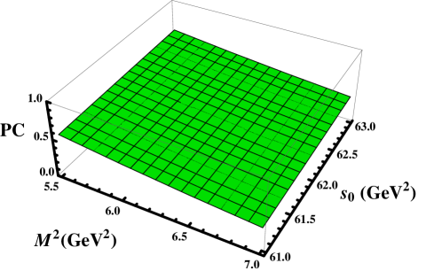
Figure 1: The pole contribution as a function of the Borel and continuum threshold parameters $M^{2}$ and $s_{0}$.

Our analysis proves that the working regions

$$M^{2}\in[5.5,~{}7]~{}\mathrm{GeV}^{2},\ s_{0}\in[61,~{}63]~{}\mathrm{GeV}^{2},$$ (11)

satisfy all aforementioned restrictions. Thus, within the region $M^{2}\in[5.5,~{}7]~{}\mathrm{GeV}^{2}$ the pole contribution decreases approximately from $58\%$ till $34\%$. A detailed picture for $\mathrm{PC}$ is presented in Fig. 1, where we plot the pole contribution as a function of $M^{2}$ and $s_{0}$. The minimum $M_{\min}^{2}$ is found from analysis of the ratio

$$R(M^{2})=\frac{\Pi^{\mathrm{DimN}}(M^{2},\ s_{0})}{\Pi(M^{2},\ s_{0})},$$ (12)

where $\Pi(M^{2},s_{0})$ is the Borel transformed and subtracted function $\Pi^{\mathrm{OPE}}(p^{2})$. In the present work as a measure of the convergence we use the sum of last three terms in OPE $\mathrm{DimN}=\mathrm{Dim(8+9+10)}$ and impose the constraint on $R(M^{2})$: the restriction $R(M_{\min}^{2})$ $\leq 0.01$ is fulfilled at $5.5\ \mathrm{GeV}^{2}$. The perturbative contribution at $M^{2}=5.5~{}\mathrm{GeV}^{2}$ amounts to $68\%$ of the full result and overshoots contribution of the nonperturbative terms. In Fig. 2 we demonstrate the dependence of the mass $m$ on $M^{2}$ and $s_{0}$, where weak residual effects of these parameters are seen.

Our results for $m$ and $f$ read:

$$m = (7105~{}\pm 155)~{}\mathrm{MeV},$$

$$f = (1.0\pm 0.2)\times 10^{-2}~{}\mathrm{GeV}^{4}.$$ (13)

Theoretical errors of the mass is milder than ones of the coupling, nevertheless all these ambiguities do not exceed standard limits of sum rule computations reaching $2.2\%$ and $\pm 20\%$ of the corresponding central values, respectively.The spectroscopic parameters of the axial-vector tetraquark $T_{bc}^{0}$ evaluated in this section form a basis for our further investigations.

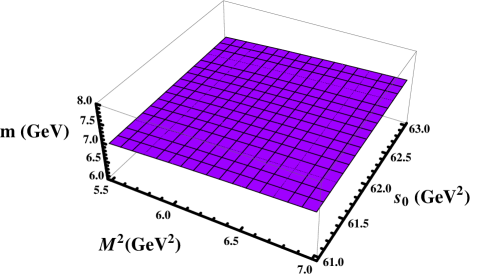
Figure 2: The same as in Fig. 1, but for the mass of the tetraquark $T_{bc}^{0}$.

III Semileptonic decays $T_{bc}^{0}\rightarrow T_{cc}^{+}l\overline{\nu}_{l}$

As it has been emphasized above for $m=7105~{}\mathrm{MeV}$ the tetraquark $T_{bc}^{0}$ is stable against the strong and electromagnetic interactions, because then $m$ resides $85/190~{}\mathrm{MeV}$ and $45~{}\mathrm{MeV}$ below the strong and electromagnetic thresholds, respectively. The semileptonic decays $T_{bc}^{0}\rightarrow T_{cc}^{+}l\overline{\nu}_{l}$ of the tetraquark $T_{bc}^{0}$ are caused by weak transition $b\rightarrow W^{-}c\rightarrow cl\overline{\nu}$ of the heavy $b$-quark. It is not difficult to see, that due to large mass difference between the tetraquarks $T_{bc}^{0}$ and $T_{cc}^{+}$, all of the transitions $T_{bc}^{0}\rightarrow T_{cc}^{+}l\overline{\nu}_{l}$ with $l=e,\ \mu$ and $\tau$ are kinematically allowed processes. We restrict ourselves by considering only the dominant process $b\rightarrow W^{-}c$, because due to smallness of the Cabibbo-Kobayashi-Maskawa (CKM) matrix element $|V_{bu}|^{2}/|V_{bc}|^{2}$ $\simeq 0.01$ the decay $b\rightarrow W^{-}u$ is suppressed relative to the first one.

At the tree-level, the transition $b\rightarrow W^{-}c$ is described by means of the effective Hamiltonian

$$\mathcal{H}^{\mathrm{eff}}=\frac{G_{F}}{\sqrt{2}}V_{bc}\overline{c}\gamma_{\mu}(1-\gamma_{5})b\overline{l}\gamma^{\mu}(1-\gamma_{5})\nu_{l}.$$ (14)

Here $G_{F}$ is the Fermi coupling constant, and $V_{bc}$ is the element of the CKM matrix. After substituting $\mathcal{H}^{\mathrm{eff}}$ between the initial and final tetraquark fields and factoring out the leptonic piece we get the matrix element of the current

$$J_{\mu}^{\mathrm{tr}}=\overline{c}\gamma_{\mu}(1-\gamma_{5})b,$$ (15)

which has to be calculated in terms of the weak form factors $G_{i}(q^{2})$: they parameterize the long-distance dynamics of the transition

$$\langle T_{cc}^{+}(p^{\prime})|J_{\mu}^{\mathrm{tr}}|T_{bc}^{0}(p,\epsilon)\rangle=\overline{m}G_{0}(q^{2})\epsilon_{\mu}+\frac{G_{1}(q^{2})}{\overline{m}}(\epsilon p^{\prime})P_{\mu}$$

$$+\frac{G_{2}(q^{2})}{\overline{m}}(\epsilon p^{\prime})q_{\mu}+i\frac{G_{3}(q^{2})}{\overline{m}}\varepsilon_{\mu\nu\alpha\beta}\epsilon^{\nu}p^{\alpha}p^{\prime}{}^{\beta}.$$ (16)

In Eq. (16) $\ p$ and $\epsilon$ are the momentum and polarization vector of the $T_{bc}^{0}$, $p^{\prime}$ is the momentum of the scalar tetraquark $T_{cc}^{+}$. Here we also use the shorthand notations $\overline{m}=m+m_{T}$ and $P_{\mu}=p_{\mu}^{\prime}+p_{\mu}$ with $m_{T}$ being the mass of the final-state tetraquark. The $q_{\mu}=p_{\mu}-p_{\mu}^{\prime}$ is the momentum transferred to the leptons changing within the limits $m_{l}^{2}\leq q^{2}\leq(m-m_{T})^{2}$, where $m_{l}$ is the mass of the lepton $l$.

The form factors $G_{i}(q^{2})$ are key quantities to be extracted from the sum rules. To this end, we consider the following three-point correlation function:

$$\Pi_{\mu\nu}(p,p^{\prime}) = i^{2}\int d^{4}xd^{4}ye^{i(p^{\prime}y-px)}$$ (17)

$$\times\langle 0|\mathcal{T}\{J^{T}(y)J_{\mu}^{\mathrm{tr}}(0)J_{\nu}^{{}^{\dagger}}(x)\}|0\rangle,$$

where $J_{\nu}(x)$ and $J^{T}(y)$ are the interpolating currents corresponding to the states $T_{bc}^{0}$ and $T_{cc}^{+}$, respectively. The current $J_{\nu}(x)$ has been introduced by Eq. (2). The interpolating current for the state$T_{cc}^{+}$ is given by the expression:

$$J^{T}(y)=\epsilon\widetilde{\epsilon}[c_{b}^{T}(y)C\gamma_{\alpha}c_{c}(y)][\overline{u}_{d}(y)\gamma^{\alpha}C\overline{d}_{e}^{T}(y)],$$ (18)

where $\epsilon\widetilde{\epsilon}=\epsilon^{abc}\epsilon^{ade}$. Here, $\epsilon^{abc}[c_{b}^{T}C\gamma_{\alpha}c_{c}]$ and $\epsilon^{ade}[\overline{u}_{d}\gamma^{\alpha}C\overline{d}_{e}^{T}]$ are the axial-vector diquark and antidiquark, respectively. Then the scalar designation of the final tetraquark $T_{cc}^{+}$ stems naturally from the internal structure of the initial four-quark state $T_{bc}^{0}$, which is the axial-vector particle composed of the scalar diquark $b^{T}C\gamma_{5}c$ and axial-vector antidiquark $\overline{u}\gamma_{\mu}C\overline{d}^{T}$. The semileptonic decay $T_{bc}^{0}\rightarrow T_{cc}^{+}+W^{-}$ runs through $b\rightarrow W^{-}c$, which transforms the scalar diquark $bc$ to the final axial-vector $cc$, leaving, at the same time, unchanged the initial light antidiquark; the light axial-vector antidiquark $\overline{u}\overline{d}$ appears both in the initial and final states. The designation of $T_{cc}^{+}$ as an axial-vector requires $\overline{u}\overline{d}$ to be a scalar, which implies additional spin-rearrangement in the initial axial-vector $\overline{u}\overline{d}$ diquark, which evidently suppresses the corresponding process.

Our strategy to derive sum rules for the form factors $G_{i}(q^{2})$ is the same as in all of this kind studies. In fact, to determine the phenomenological side of the sum rule $\Pi_{\mu\nu}^{\mathrm{Phys}}(p,p^{\prime})$ we express the correlation function $\Pi_{\mu\nu}(p,p^{\prime})$ in terms of the spectroscopic parameters of particles involving into the decay process. Afterwards we find the QCD side (or OPE) side of the sum rules $\Pi_{\mu\nu}^{\mathrm{OPE}}(p,p^{\prime})$ by computing the same correlation function in terms of quark propagators. By matching the obtained results and utilizing the quark-hadron duality assumption we extract sum rules and evaluate the physical quantities of interest. Because the quark propagators contain quark, gluon and mixed vacuum condensates, the sum rules express the physical quantities as functions of nonperturbative parameters.

In the context of this approach the function $\Pi_{\mu\nu}^{\mathrm{Phys}}(p,p^{\prime})$ can be recast into the form

$$\Pi_{\mu\nu}^{\mathrm{Phys}}(p,p^{\prime})=\frac{\langle 0|J^{T}|T_{cc}^{+}(p^{\prime})\rangle\langle T_{cc}^{+}(p^{\prime})|J_{\mu}^{\mathrm{tr}}|T_{bc}^{0}(p,\epsilon)\rangle}{(p^{2}-m^{2})(p^{\prime 2}-m_{T}^{2})}$$

$$\times\langle T_{bc}^{0}(p,\epsilon)|J_{\nu}^{{}^{\dagger}}|0\rangle+\ldots,$$ (19)

where $m_{T}$ is the mass of $T_{cc}^{+}$. In the expression above we take into account contribution appearing due to only the ground-state particles, denoting contributions of the higher resonances and continuum states by the dots.

Transformation of the ground-state term in $\Pi_{\mu\nu}^{\mathrm{Phys}}(p,p^{\prime})$ can be completed by detailing the matrix elements in its expression. The matrix element of $T_{bc}^{0}$ and the matrix element for the transition $\langle T_{cc}^{+}(p^{\prime})|J_{\mu}^{\mathrm{tr}}|T_{bc}^{0}(p,\epsilon)\rangle$ are given by Eqs. (4) and (16), respectively. The remaining quantity

$$\langle 0|J^{T}|T_{cc}^{+}(p^{\prime})\rangle=m_{T}f_{T},$$ (20)

has a simple form and depends only on the mass and coupling $f_{T}$ of the tetraquark $T_{cc}^{+}$. Benefiting from these explicit formulas, for $\Pi_{\mu\nu}^{\mathrm{Phys}}(p,p^{\prime},q^{2})$ we obtain

$$\Pi_{\mu\nu}^{\mathrm{Phys}}(p,p^{\prime},q^{2})=\frac{fmf_{T}m_{T}}{(p^{2}-m^{2})(p^{\prime 2}-m_{T}^{2})}$$

$$\times\left\{\overline{m}G_{0}(q^{2})\left(-g_{\mu\nu}+\frac{p_{\mu}p_{\nu}}{m^{2}}\right)+\left[\frac{G_{1}(q^{2})}{\overline{m}}P_{\mu}\right.\right.$$

$$\left.+\frac{G_{2}(q^{2})}{\overline{m}}q_{\mu}\right]\left(-p_{\nu}^{\prime}+\frac{m^{2}+m_{T}^{2}-q^{2}}{2m^{2}}p_{\nu}\right)$$

$$\left.-i\frac{G_{3}(q^{2})}{\overline{m}}\varepsilon_{\mu\nu\alpha\beta}p^{\alpha}p^{\prime}{}^{\beta}\right\}+\ldots.$$ (21)

The function $\Pi_{\mu\nu}^{\mathrm{OPE}}(p,p^{\prime})$ forms the second side of the sum rules:

$$\Pi_{\mu\nu}^{\mathrm{OPE}}(p,p^{\prime})=i^{2}\epsilon\widetilde{\epsilon}\int d^{4}xd^{4}ye^{i(p^{\prime}y-px)}\left(\mathrm{Tr}\left[\gamma^{\alpha}\widetilde{S}_{d}^{b^{\prime}e}(x-y)\right.\right.$$

$$\left.\left.\times\gamma_{\nu}S_{u}^{a^{\prime}d}(x-y)\right]-\mathrm{Tr}\left[\gamma^{\alpha}\widetilde{S}_{d}^{a^{\prime}e}(x-y)\gamma_{\nu}S_{u}^{b^{\prime}d}(x-y)\right]\right)$$

$$\times\left(\mathrm{Tr}\left[\gamma_{\mu}(1-\gamma_{5})S_{b}^{ia^{\prime}}(-x)\gamma_{5}\widetilde{S}_{c}^{bb^{\prime}}(y-x)\gamma_{\alpha}S_{c}^{ci}(y)\right]\right.$$

$$\left.-\mathrm{Tr}\left[\gamma_{\mu}(1-\gamma_{5})S_{b}^{ia^{\prime}}(-x)\gamma_{5}\widetilde{S}_{c}^{cb^{\prime}}(y-x)\gamma_{\alpha}S_{c}^{bi}(y)\right]\right).$$

(22)

The required sum rules for the form factors $G_{i}(q^{2})$ can be obtained by equating invariant amplitudes corresponding to the same Lorentz structures both in $\Pi_{\mu\nu}^{\mathrm{Phys}}(p,p^{\prime},q^{2})$ and $\Pi_{\mu\nu}^{\mathrm{OPE}}(p,p^{\prime})$. Because in the three-point sum rules the invariant amplitudes are functions of $p^{\prime 2}$ and $p^{2}$, to suppress contributions of higher resonances and continuum states we have to apply the double Borel transformation over these variables. As a result, the final expressions depend on a set of Borel parameters $\mathbf{M}^{2}=(M_{1}^{2},\ M_{2}^{2})$. The continuum subtraction is performed in two channels using two continuum parameters $\mathbf{s}_{0}=(s_{0},\ s_{0}^{\prime})$. The form factor $G_{0}(q^{2})$ is obtained by using the structure $g_{\mu\nu}$ and reads:

$$G_{0}(\mathbf{M}^{2},\ \mathbf{s}_{0},~{}q^{2})=\frac{1}{\overline{m}fmf_{T}m_{T}}\int_{\mathcal{M}^{2}}^{s_{0}}ds\int_{4m_{c}^{2}}^{s_{0}^{\prime}}ds^{\prime}$$

$$\times\rho_{0}(s,s^{\prime},q^{2})e^{(m^{2}-s)/M_{1}^{2}}e^{(m_{T}^{2}-s^{\prime})/M_{2}^{2}}.$$ (23)

The form factors $G_{i}(q^{2})$ ($i=1,2,3$) are derived employing other Lorentz structures in the correlation functions:

$$G_{i}(\mathbf{M}^{2},\ \mathbf{s}_{0},~{}q^{2})=\frac{\overline{m}}{fmf_{T}m_{T}}\int_{\mathcal{M}^{2}}^{s_{0}}ds\int_{4m_{c}^{2}}^{s_{0}^{\prime}}ds^{\prime}$$

$$\times\rho_{i}(s,s^{\prime},q^{2})e^{(m^{2}-s)/M_{1}^{2}}e^{(m_{T}^{2}-s^{\prime})/M_{2}^{2}}.$$ (24)

The sum rules (23) and (24) are written down in terms of the spectral densities $\rho_{i}(s,s^{\prime},q^{2})$ which are proportional to the imaginary parts of the corresponding terms in $\Pi_{\mu\nu}^{\mathrm{OPE}}(p,p^{\prime})$. They contain the perturbative and nonperturbative contributions, and are calculated with dimension-5 accuracy.

Quantity	Value
$m_{T}$	$(3845~{}\pm 175)~{}\mathrm{MeV}$
$f_{T}$	$(1.16\pm 0.26)\times 10^{-2}~{}\mathrm{GeV}^{4}$
$m_{e}$	$0.511~{}\mathrm{MeV}$
$m_{\mu}$	$105.658~{}\mathrm{MeV}$
$m_{\tau}$	$(1776.82~{}\pm 0.16)~{}\mathrm{MeV}$
$G_{F}$	$1.16637\times 10^{-5}~{}\mathrm{GeV}^{-2}$
$|V_{bc}|$	$(42.2\pm 0.08)\times 10^{-3}$

Table 1: The mass and coupling of the final-state tetraquark $T_{cc}^{+}$ and other parameters used in numerical computations.

To compute the weak form factors $G_{i}(\mathbf{M}^{2},\ \mathbf{s}_{0},~{}q^{2})$ we need numerical values of parameters which enter to the sum rules. The vacuum condensates are given in Eq. (10), whereas the spectroscopic parameters of the tetraquark $T_{cc}^{+}$ is borrowed from our work Agaev:2019qqn . The mass and coupling of the initial particle $T_{bc}^{0}$ have been calculated in the previous section; these and other parameters are collected in Table 1. In computations, we impose on the auxiliary parameters $\mathbf{M}^{2}$ and $\mathbf{s}_{0}$ the same constraints as in the mass calculations: the set ($M_{1}^{2},\ s_{0}$) for the initial particle channel is determined by Eq. (11), whereas the set ($M_{2}^{2},\ s_{0}^{\prime}$) for $T_{cc}^{+}$ is chosen in the form Agaev:2019qqn

$$M_{2}^{2}\in[3,\ 4]~{}\mathrm{GeV}^{2},\ s_{0}^{\prime}\in[19,\ 21]~{}\mathrm{GeV}^{2}.$$ (25)

Results of sum rule calculations in the case of $G_{0}(q^{2})$, as an example, are shown in Fig. 3.

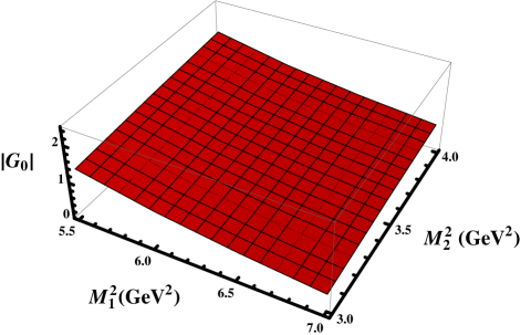
Figure 3: The form factor $|G_{0}|=|G_{0}(5~{}\mathrm{GeV}^{2})|$ as a function of the Borel parameters $M_{1}^{2}$ and $M_{2}^{2}$ at $s_{0}=62~{}\mathrm{GeV}^{2}$ and $s_{0}^{\prime}=20~{}\mathrm{GeV}^{2}$.

The similar predictions have been obtained for the remaining form factors as well. The sum rule results for the functions $G_{i}(q^{2})$ are necessary, but not enough to calculate the partial width of the process $T_{bc}^{0}\rightarrow T_{cc}^{+}l\overline{\nu}_{l}$. The reason is that these form factors determine its differential decay rate $d\Gamma/dq^{2}$ (see, Appendix in Ref. Agaev:2018khe ). The partial width $\Gamma$ should be found by integrating $d\Gamma/dq^{2}$ over $q^{2}$ within limits allowed by the kinematical constraints $m_{l}^{2}\leq q^{2}\leq(m-m_{T})^{2}$. But sum rules do not cover all this region, and give reliable results within the limits $m_{l}^{2}\leq q^{2}\leq 8\ ~{}\mathrm{GeV}^{2}$. Therefore, one has to introduce the model functions $F_{i}(q^{2})$, which at accessible for the sum rule computations $q^{2}$ coincide with $G_{i}(q^{2})$, but can be extrapolated to the whole integration region.

The fit functions

$$F_{i}(q^{2})=F_{0}^{i}\exp\left[c_{1}^{i}\frac{q^{2}}{m_{\mathrm{fit}}^{2}}+c_{2}^{i}\left(\frac{q^{2}}{m_{\mathrm{fit}}^{2}}\right)^{2}\right],$$ (26)

are convenient for these purposes. Here $F_{0}^{i},~{}c_{1}^{i},\$ $c_{2}^{i}$ and $m_{\mathrm{fit}}^{2}$ are the fit parameters numerical values of which are collected in Table 2.

$F_{i}(q^{2})$	$F_{0}^{i}$	$c_{1}^{i}$	$c_{2}^{i}$	$m^{2}_{\mathrm{fit}}\ (\mathrm{GeV}^{2})$
$F_{0}(q^{2})$	$-0.92$	$0.43$	$-9.36$	$50.48$
$F_{1}(q^{2})$	$10.87$	$2.83$	$3.69$	$50.48$
$F_{2}(q^{2})$	$-2.61$	$0.32$	$4.44$	$50.48$
$F_{3}(q^{2})$	$-13.79$	$2.06$	$3.31$	$50.48$

Table 2: The parameters of the fit functions $F_{i}(q^{2})$.

Our predictions for the partial width of the semileptonic decay channels are:

$$\Gamma(T_{bc}^{0} \rightarrow T_{cc}^{+}e^{-}\overline{\nu}_{e})=(1.44\pm 0.35)\times 10^{-10}\ \mathrm{MeV},$$

$$\Gamma(T_{bc}^{0} \rightarrow T_{cc}^{+}\mu^{-}\overline{\nu}_{\mu})=(1.43\pm 0.34)\times 10^{-10}\ \mathrm{MeV},$$

$$\Gamma(T_{bc}^{0} \rightarrow T_{cc}^{+}\tau^{-}\overline{\nu}_{\tau})=(4.3\pm 1.1)\times 10^{-11}\ \mathrm{MeV}.$$

Results (LABEL:eq:Results) obtained in this section constitute an important part of the full width of $T_{bc}^{0}$, and will be used below for its evaluation.

IV Two-body weak decays $T_{bc}^{0}\rightarrow T_{cc}^{+}\pi^{-}(K^{-},\ D^{-},\ D_{s}^{-})$

The two-body weak decays $T_{bc}^{0}\rightarrow T_{cc}^{+}\pi^{-}(K^{-},\ D^{-},\ D_{s}^{-})$ of the tetraquark $T_{bc}^{0}$ can be considered in the context of the QCD factorization approach, which allows one to write amplitudes and calculate widths of these processes. This method was successfully applied to study two-body weak decays of the conventional mesons Beneke:1999br ; Beneke:2000ry , and is used here to investigate two-body decays of the tetraquark $T_{bc}^{0}$, when one of the final particles is an exotic meson.

We consider in a detailed form only the decay $T_{bc}^{0}\rightarrow T_{cc}^{+}\pi^{-}$ , and write down final predictions for remaining channels. At the quark level, the effective Hamiltonian for the this decay is given by the expression

$$\widetilde{\mathcal{H}}^{\mathrm{eff}}=\frac{G_{F}}{\sqrt{2}}V_{bc}V_{ud}^{\ast}\left[c_{1}(\mu)Q_{1}+c_{2}(\mu)Q_{2}\right],$$ (28)

where

$$Q_{1} = \left(\overline{d}_{i}u_{i}\right)_{\mathrm{V-A}}\left(\overline{c}_{j}b_{j}\right)_{\mathrm{V-A}},$$

$$Q_{2} = \left(\overline{d}_{i}u_{j}\right)_{\mathrm{V-A}}\left(\overline{c}_{j}b_{i}\right)_{\mathrm{V-A}},$$ (29)

and $i$ , $j$ are the color indices. Here $c_{1}(\mu)$ and $c_{2}(\mu)$ are the short-distance Wilson coefficients evaluated at the scale $\mu$ at which the factorization is assumed to be correct. The shorthand notation $\left(\overline{q}_{1}q_{2}\right)_{\mathrm{V-A}}$ in Eq. (29) means

$$\left(\overline{q}_{1}q_{2}\right)_{\mathrm{V-A}}=\overline{q}_{1}\gamma_{\mu}(1-\gamma_{5})q_{2}.$$ (30)

The amplitude of this decay can be written down in the following factorized form

$$\mathcal{A} = \frac{G_{F}}{\sqrt{2}}V_{bc}V_{ud}^{\ast}a_{1}(\mu)\langle\pi^{-}(q)|\left(\overline{d}_{i}u_{i}\right)_{\mathrm{V-A}}|0\rangle$$ (31)

$$\times\langle T_{cc}^{+}(p^{\prime})|\left(\overline{c}_{j}b_{j}\right)_{\mathrm{V-A}}|T_{bc}^{0}(p,\epsilon)\rangle$$

where

$$a_{1}(\mu)=c_{1}(\mu)+\frac{1}{N_{c}}c_{2}(\mu),$$ (32)

and $N_{c}$ is the number of quark colors. The amplitude $\mathcal{A}$ describes the process in which the pion $\pi^{-}$ is generated directly from the color-singlet current $\left(\overline{d}_{i}u_{i}\right)_{\mathrm{V-A}}$. The matrix element $\langle T_{cc}^{+}(p^{\prime})|\left(\overline{c}_{j}b_{j}\right)_{\mathrm{V-A}}|T_{bc}^{0}(p,\epsilon)\rangle$ has been introduced by Eq. (16), whereas the matrix element of the pion in given by the expression

$$\langle\pi^{-}(q)|\left(\overline{d}_{i}u_{i}\right)_{\mathrm{V-A}}|0\rangle=if_{\pi}q_{\mu},$$ (33)

and is determined by its decay constant $f_{\pi}$.

Then, it is not difficult to see that $\mathcal{A}$ takes the form

$$\mathcal{A}=i\frac{G_{F}}{\sqrt{2}}f_{\pi}V_{bc}V_{ud}^{\ast}a_{1}(\mu)(\epsilon p^{\prime})\left[-\overline{m}G_{0}(q^{2})\right.$$

$$\left.+\frac{G_{1}(q^{2})}{\overline{m}}Pq+\frac{G_{2}(q^{2})}{\overline{m}}m_{\pi}^{2}\right].$$ (34)

The width of the decay $T_{bc}^{0}\rightarrow T_{cc}^{+}\pi^{-}$ is

$$\Gamma\left(T_{bc}^{0}\rightarrow T_{cc}^{+}\pi^{-}\right)=\frac{G_{F}^{2}f_{\pi}^{2}}{48\pi m^{2}}|V_{bc}|^{2}|V_{ud}|^{2}a_{1}^{2}(\mu)$$

$$\times\lambda^{3}(m^{2},m_{T}^{2},m_{\pi}^{2})\left[\overline{m}^{2}|G_{0}|^{2}+\frac{|G_{1}|^{2}}{\overline{m}^{2}}(m^{2}-m_{T}^{2})^{2}\right.$$

$$+\frac{|G_{2}|^{2}}{\overline{m}^{2}}m_{\pi}^{4}-2\operatorname{Re}\left[G_{0}G_{1}^{\ast}\right](m^{2}-m_{T}^{2})$$

$$\left.-2\operatorname{Re}\left[G_{0}G_{2}^{\ast}\right]m_{\pi}^{2}+2\operatorname{Re}\left[G_{1}G_{2}^{\ast}\right]\frac{(m^{2}-m_{T}^{2})m_{\pi}^{2}}{\overline{m}^{2}}\right],$$

(35)

where the weak form factors $G_{i}(q^{2})$ ($i=0,1,2$) are taken at $q^{2}=m_{\pi}^{2}$. In Eq. (35) the function $\lambda(m^{2},m_{T}^{2},m_{\pi}^{2})$ is given by the formula

$$\lambda\left(m^{2},m_{T}^{2},m_{\pi}^{2}\right)=\frac{1}{2m}\left[m^{4}+m_{T}^{4}+m_{\pi}^{4}\right.$$

$$\left.-2\left(m^{2}m_{T}^{2}+m^{2}m_{\pi}^{2}+m_{T}^{2}m_{\pi}^{2}\right)\right]^{1/2}.$$ (36)

The similar analysis can be performed for other decays $T_{bc}^{0}\rightarrow T_{cc}^{+}(K^{-},D^{-},D_{s}^{-})$ as well: relevant expressions can by obtained from (35) using the spectroscopic parameters of the mesons $K^{-},D^{-},$ and $D_{s}^{-}$, and by replacements $V_{ud}\rightarrow V_{us}$, $V_{cd}$, and $V_{cs}$, respectively.

Numerical computations can be carried out after fixing the spectroscopic parameters of the final-state pseudoscalar mesons, weak form factors, and CKM matrix elements. The masses and decay constants of the final-state pseudoscalar mesons are presented in Table 3. The weak form factors $G_{i}(q^{2})$ ($i=0,1,2,3$), which are crucial parts of calculations, have been obtained in the previous section. For CKM matrix elements we use $|V_{ud}|=0.97420\pm 0.00021$, $|V_{us}|=0.2243\pm 0.0005$, $|V_{cd}|=0.218\pm 0.004$ and $|V_{cs}|=0.997\pm 0.017$. The values of the Wilson coefficients $c_{1}(m_{b}),\$and $c_{2}(m_{b})$ with next-to-leading order QCD corrections were presented in Refs. Buras:1992zv ; Ciuchini:1993vr ; Buchalla:1995vs

$$c_{1}(m_{b})=1.117,\ c_{2}(m_{b})=-0.257.$$ (37)

Quantity	Value
$m_{\pi}$	$139.570~{}\mathrm{MeV}$
$m_{K}$	$(493.677\pm 0.016)~{}\mathrm{MeV}$
$m_{D}$	$(1869.61\pm 0.10)~{}\mathrm{MeV}$
$m_{D_{s}}$	$(1968.30\pm 0.11)~{}\textrm{MeV}$
$f_{\pi}$	$131~{}\text{MeV}$
$f_{K}$	$(155.72\pm 0.51)~{}\text{MeV}$
$f_{D}$	$(203.7\pm 4.7)~{}\text{MeV}$
$f_{D_{s}}$	$(257.8\pm 4.1)~{}\text{MeV}$

Table 3: Masses and decay constants of the pseudoscalar mesons.

For the decay $T_{bc}^{0}\rightarrow T_{cc}^{+}\pi^{-}$, calculations lead to the following result

$$\Gamma\left(T_{bc}^{0}\rightarrow T_{cc}^{+}\pi^{-}\right)=\left(1.73\pm 0.38\right)\times 10^{-11}\ \mathrm{MeV}.$$

(38)

Width of this decay is smaller than widths of the semileptonic decays, but is comparable with them. For the remaining weak nonleptonic decays of the tetraquark $T_{bc}^{0}$ we get

$$\Gamma\left(T_{bc}^{0}\rightarrow T_{cc}^{+}K^{-}\right)=\left(1.27\pm 0.26\right)\times 10^{-12}~{}\mathrm{MeV},$$

$$\Gamma\left(T_{bc}^{0}\rightarrow T_{cc}^{+}D^{-}\right)=\left(1.65\pm 0.35\right)\times 10^{-12}~{}\mathrm{MeV},$$

$$\Gamma\left(T_{bc}^{0}\rightarrow T_{cc}^{+}D_{s}^{-}\right)=\left(4.74\pm 0.99\right)\times 10^{-11}~{}\mathrm{MeV}.$$

(39)

It is seen that partial widths only of the nonleptonic weak decays $T_{bc}^{0}\rightarrow T_{cc}^{+}D_{s}^{-}$ and $T_{bc}^{0}\rightarrow T_{cc}^{+}\pi^{-}$ are comparable with widths of the semileptonic modes  (LABEL:eq:Results); contribution to the full width of $T_{bc}^{0}$ coming from other two weak decays is neglidible.

Using Eqs. (LABEL:eq:Results) and (39), it is not difficult to find the full width and mean lifetime of $T_{bc}^{0}$

$$\Gamma_{\mathrm{full}} = (3.98\pm 0.51)\times 10^{-10}~{}\mathrm{MeV},$$

$$\tau = 1.65_{-0.18}^{+0.25}\times 10^{-12}~{}\mathrm{s}.$$ (40)

Predictions for $\Gamma_{\mathrm{full}}$ and $\tau$ are among main results of the present work.

V Strong decays $T_{bc}^{0}\rightarrow B^{\ast-}D^{+}$ and $T_{bc}^{0}\rightarrow\overline{B}^{\ast 0}D^{0}$

Calculations of the mass of the tetraquark $T_{bc}^{0}$, performed in Section II, due to uncertainties of the sum rule method do not exclude also prediction $m=7260~{}\mathrm{MeV}$. In this scenario $T_{bc}^{0}$ is strong-interaction unstable particle and decays to conventional mesons $B^{\ast-}D^{+}$ and $\overline{B}^{\ast 0}D^{0}$. It is worth noting that $m=7260~{}\mathrm{MeV}$ is below the thresholds for strong decays $T_{bc}^{0}\rightarrow B^{-}D^{\ast+}$ and $T_{bc}^{0}\rightarrow\overline{B}^{0}D^{\ast 0}$, which forbids kinematically these processes. Below we present in a detailed form our analysis of the decay $T_{bc}^{0}\rightarrow B^{\ast-}D^{+}$ and provide final predictions for $T_{bc}^{0}\rightarrow\overline{B}^{\ast 0}D^{0}$.

In the context of the QCD three-point sum rule method the strong decay $T_{bc}^{0}\rightarrow B^{\ast-}D^{+}$ can be studied using the correlation function

$$\widetilde{\Pi}_{\mu\nu}(p,p^{\prime}) = i^{2}\int d^{4}xd^{4}ye^{i(p^{\prime}y-px)}\langle 0|\mathcal{T}\{J_{\mu}^{B^{\ast}}(y)$$ (41)

$$\times J^{D}(0)J_{\nu}^{\dagger}(x)\}|0\rangle.$$

Here $J_{\nu}(x)$,$\ J^{D}(x)$ and $J_{\mu}^{B^{\ast}}(x)$ are the interpolating currents for the tetraquark $T_{bc}^{0}$ and mesons $D^{+}$ and $B^{\ast-}$, respectively. The $J_{\nu}(x)$ is given by Eq. (2), whereas for the remaining two currents we use

$$J_{\mu}^{B^{\ast}}(x)=\overline{u}^{i}(x)\gamma_{\mu}b^{i}(x),\ \ J^{D}(x)=\overline{d}^{j}(x)i\gamma_{5}c^{j}(x).$$ (42)

The 4-momenta of the tetraquark $T_{bc}^{0}$ and meson $B^{\ast-}$ are $p$ and $p^{\prime}$, therefore, the momentum of the meson $D^{+}$ is $q=p-p^{\prime}$.

We follow the standard recipes and calculate the correlation function $\widetilde{\Pi}_{\mu\nu}(p,p^{\prime})$ using both the physical parameters of the particles involved into the process, and quark propagators. Separating the ground-state contribution from ones due to higher resonances and continuum states, for the physical side of the sum rule, we get

$$\widetilde{\Pi}_{\mu\nu}^{\mathrm{Phys}}(p,p^{\prime})=\frac{\langle 0|J_{\mu}^{B^{\ast}}|B^{\ast-}(p^{\prime},\epsilon^{\prime})\rangle\langle 0|J^{D}|D^{+}(q)\rangle}{(p^{\prime 2}-m_{B^{\ast}}^{2})(q^{2}-m_{D}^{2})}$$

$$\times\frac{\langle D^{+}(q)B^{\ast-}(p^{\prime},\epsilon^{\ast\prime})|T_{bc}^{0}(p,\epsilon)\rangle\langle T_{bc}^{0}(p,\epsilon^{\ast})|J_{\nu}^{\dagger}|0\rangle}{(p^{2}-m^{2})}+\ldots$$

(43)

The function $\widetilde{\Pi}_{\mu\nu}^{\mathrm{Phys}}(p,p^{\prime})$ can be simplified by expressing the matrix elements in terms of the tetraquark and mesons’ physical parameters. The matrix element $\langle T_{bc}^{0}(p,\epsilon^{\ast})|J_{\nu}^{\dagger}|0\rangle$ can be found using Eq. (4). We introduce also the matrix elements of the final-state mesons

$$\langle 0|J^{D}|D^{+}\rangle = \frac{m_{D}^{2}f_{D}}{m_{c}},\$$

$$\langle 0|J_{\mu}^{B^{\ast}}|B^{\ast-}(p^{\prime},\epsilon^{\prime})\rangle = m_{B^{\ast}}f_{B^{\ast}}\epsilon_{\mu}^{\prime}.$$ (44)

Here $m_{D}$,$\ m_{B^{\ast}}$ and $f_{D}$, $f_{B^{\ast}}$ are the masses and decay constants of the mesons $D^{+}$ and $B^{\ast-}$, respectively. In Eq. (44) $\epsilon_{\mu}^{\prime}$ is the polarization vector of the meson $B^{\ast-}$. We model $\langle D^{+}(q)B^{\ast-}(p^{\prime},\epsilon^{\ast\prime})|T_{bc}^{0}(p,\epsilon)\rangle$ in the form

$$\langle D^{+}(q)B^{\ast-}(p^{\prime},\epsilon^{\ast\prime})|T_{bc}^{0}(p,\epsilon)\rangle=g_{1}(q^{2})\left[(p\cdot p^{\prime})\right.$$

$$\left.\times(\epsilon\cdot\epsilon^{\ast\prime})-(p\cdot\epsilon^{\ast\prime})(p^{\prime}\cdot\epsilon)\right]$$ (45)

and denote by $g_{1}(q^{2})$ the strong form factor corresponding to the vertex $T_{bc}^{0}B^{\ast-}D^{+}.$ Then, it is not difficult to see that

$$\widetilde{\Pi}_{\mu\nu}^{\mathrm{Phys}}(p,p^{\prime})=g_{1}\frac{m_{D}^{2}m_{B^{\ast}}mff_{D}f_{B^{\ast}}}{m_{c}(p^{2}-m^{2})(p^{\prime 2}-m_{B^{\ast}}^{2})}$$

$$\times\frac{1}{(q^{2}-m_{D}^{2})}\left[\frac{1}{2}(m^{2}+m_{B^{\ast}}^{2}-q^{2})g_{\mu\nu}-p_{\mu}p_{\nu}^{\prime}\right]+\ldots$$

(46)

The correlation function $\widetilde{\Pi}_{\mu\nu}^{\mathrm{Phys}}(p,p^{\prime})$ has Lorentz structures proportional to $g_{\mu\nu}$ and $p_{\mu}p_{\nu}^{\prime}$. We work with the invariant amplitude $\widetilde{\Pi}^{\mathrm{Phys}}(p^{2},p^{\prime 2},q^{2})$ that corresponds to the structure $\sim g_{\mu\nu}$. The double Borel transformation of this amplitude over variables $p^{2}$ and $p^{\prime 2}$ forms the phenomenological side of the sum rule.

To find the QCD side of the three-point sum rule, we calculate $\widetilde{\Pi}_{\mu\nu}(p,p^{\prime})$ in terms of the quark propagators and get

$$\Pi_{\mu\nu}^{\mathrm{OPE}}(p,p^{\prime})=\int d^{4}xd^{4}ye^{i(p^{\prime}y-px)}\left\{\mathrm{Tr}\left[\gamma_{5}S_{c}^{jb}(-x)\gamma_{5}\right.\right.$$

$$\left.\times\widetilde{S}_{b}^{ia}(y-x)\gamma_{\mu}\widetilde{S}_{u}^{ai}(x-y)\gamma_{\nu}S_{d}^{bj}(x)\right]-\mathrm{Tr}\left[\gamma_{5}S_{c}^{jb}(-x)\right.$$

$$\left.\left.\times\gamma_{5}\widetilde{S}_{b}^{ia}(y-x)\gamma_{\mu}\widetilde{S}_{u}^{bi}(x-y)\gamma_{\nu}S_{d}^{aj}(x)\right]\right\}.$$ (47)

As in the case of the correlation function $\widetilde{\Pi}_{\mu\nu}^{\mathrm{Phys}}(p,p^{\prime})$ here, we also isolate the structure $\sim g_{\mu\nu}$ and find the amplitude $\widetilde{\Pi}^{\mathrm{OPE}}(p^{2},p^{\prime 2},q^{2})$. The standard manipulations with invariant amplitudes yield the following sum rule

$$g_{1}(q^{2})=\frac{2m_{c}}{m_{B^{\ast}}mff_{D}f_{B^{\ast}}}\frac{q^{2}-m_{D}^{2}}{m^{2}+m_{B^{\ast}}^{2}-q^{2}}$$

$$\times e^{m^{2}/M_{1}^{2}}e^{m_{B^{\ast}}^{2}/M_{2}^{2}}\widetilde{\Pi}^{\mathrm{OPE}}(\mathbf{M}^{2},\mathbf{s}_{0},q^{2}),$$ (48)

where $\mathbf{M}^{2}=(M_{1}^{2},M_{2}^{2}),$ and $\mathbf{s}_{0}=(s_{0},s_{0}^{\prime})$ are the Borel and continuum threshold parameters. Apart from $q^{2}$, the form factor $g_{1}(q^{2})$ is also a function of the Borel and continuum threshold parameters which, for simplicity, are not shown explicitly in Eq. (48). The set $\ (M_{1}^{2},s_{0})$ corresponds to initial tetraquark channel, whereas $(M_{2}^{2},s_{0}^{\prime})$ describes the channel of the heavy final meson $B^{\ast-}$. Here, $\widetilde{\Pi}^{\mathrm{OPE}}(\mathbf{M}^{2},\mathbf{s}_{0},q^{2})$ is the invariant amplitude $\widetilde{\Pi}^{\mathrm{OPE}}(p^{2},p^{\prime 2},q^{2})$ after the double Borel transformation and continuum subtraction procedures:

$$\widetilde{\Pi}^{\mathrm{OPE}}(\mathbf{M}^{2},\mathbf{s}_{0},q^{2})=\int_{(m_{b}+m_{c})^{2}}^{s_{0}}e^{-s/M_{1}^{2}}ds$$

$$\times\int_{m_{b}^{2}}^{s_{0}^{\prime}}ds^{\prime}e^{-s^{\prime}/M_{2}^{2}}\rho\left(s,s^{\prime},q^{2}\right).$$ (49)

The spectral density $\rho(s,s^{\prime},q^{2})$ is calculated as an imaginary part of the relevant amplitude and contains the vacuum condensates up to dimension 5.

The parameters, i.e., the vacuum condensates and masses of the $b$ and $c$ quarks, which are necessary for numerical computations are given by Eq. (10). The mass and coupling of the tetraquark $T_{bc}^{0}$ have been calculated in the present work. In computations we also use $m_{D^{0}}=(1864.84\pm 0.07)~{}\mathrm{MeV}$ and $f_{D^{0}}=(203.7\pm 4.7)~{}\mathrm{MeV}$, $m_{B^{\ast}}=(5325.2\pm 0.4)~{}\mathrm{MeV}$ and $f_{B^{\ast}}=(210\pm 6)~{}\mathrm{MeV}$, respectively. Parameters of the $D$ meson can be read out from Table 3. The auxiliary parameters for the $T_{bc}^{0}$ channel are chosen in accordance with Eq. (11). For the set $(M_{2}^{2},s_{0}^{\prime})$ we use the regions

$$M^{2}_{2}\in[4.5,~{}5.5]~{}\mathrm{GeV}^{2},\ s_{0}^{\prime}\in[32,~{}34]~{}\mathrm{GeV}^{2}.$$ (50)

The sum rule method for $g_{1}(q^{2})$ gives reliable predictions only for $q^{2}<0$. Therefore, we introduce a variable $Q^{2}=-q^{2}$ and denote the new function as $g_{1}(Q^{2})$. The width of the decay $T_{bc}^{0}\rightarrow B^{\ast-}D^{+}$ has to be computed using the strong form factor at the mass shell of the $D^{+}$ meson $q^{2}=m_{D}^{2}$. This point is not accessible to sum rule computations, but the problem can be solved by employing a fit function $\mathcal{G}_{1}(Q^{2})$, which at the momenta $Q^{2}>0$ coincides with QCD sum rule predictions, but can be extrapolated to the region of $Q^{2}<0$. Then, using the interpolating function $\mathcal{G}_{1}(Q^{2}),$one can find $g_{1}(-m_{D}^{2})$. The function $\mathcal{G}_{1}(Q^{2})$ does not differ from ones that we have used in Eq. (26), a difference being only in replacement of the fitting mass with the mass of the tetraquark $m_{\mathrm{fit}}^{2}\rightarrow m^{2}$

$$\mathcal{G}_{1}(Q^{2})=\mathcal{G}_{0}^{1}\mathrm{\exp}\left[\widetilde{c}_{1}^{1}\frac{Q^{2}}{m^{2}}+\widetilde{c}_{2}^{1}\left(\frac{Q^{2}}{m^{2}}\right)^{2}\right].$$ (51)

The parameters $\mathcal{G}_{0}^{1}$, $\widetilde{c}_{1}^{1}$ and $\widetilde{c}_{2}^{1}$ have been fixed from numerical analyses $\mathcal{G}_{0}^{1}=1.11$, $\widetilde{c}_{1}^{1}=14.33,$ and $\widetilde{c}_{2}^{1}=-120.69$. This function at the mass shell $Q^{2}=-m_{D}^{2}$ gives

$$g_{1}\equiv\mathcal{G}_{1}(-m_{D}^{2})=(0.25\pm 0.03)~{}\mathrm{GeV}^{-1}.$$ (52)

The width of decay $T_{bc}^{0}\rightarrow B^{\ast-}D^{+}$ is determined by the formula

$$\Gamma[T_{bc}^{0}\rightarrow B^{\ast-}D^{+}]=\frac{g_{1}^{2}m_{B^{\ast}}^{2}}{24\pi}\lambda\left(3+2\frac{\lambda^{2}}{m_{B^{\ast}}^{2}}\right),$$ (53)

where $\lambda=\lambda\left(m^{2},m_{B^{\ast}}^{2},m_{D}^{2}\right)$.

Using Eqs. (52) and  (53), one can easily calculate the width of the decay$\ T_{bc}^{0}\rightarrow B^{\ast-}D^{+}$

$$\Gamma\left[T_{bc}^{0}\rightarrow B^{\ast-}D^{+}\right]=(31.1\pm 6.2)\ \mathrm{MeV}.$$ (54)

The second process $T_{bc}^{0}\rightarrow\overline{B}^{\ast 0}D^{0}$ can be explored by the same manner. Here, we take into account that interpolating currents have the following forms

$$J_{\mu}^{\overline{B}^{\ast 0}}(x)=\overline{d}^{i}(x)\gamma_{\mu}b^{i}(x),\ \ J^{D^{0}}(x)=\overline{u}^{j}(x)i\gamma_{5}c^{j}(x).$$ (55)

The remaining operations are standard manipulations in the context of the sum rule method. Therefore, we do not see a necessity to provide a detailed information on them. Let us note only that the fit function $\mathcal{G}_{2}(Q^{2})$ has the parameters $\mathcal{G}_{0}^{1}=1.11$, $\widetilde{c}_{1}^{2}=14.40$, and $\widetilde{c}_{2}^{2}=-121.11.$ At the mass shell of the meson $D^{0}$ for the strong coupling we get

$$g_{2}\left(-m_{D^{0}}^{2}\right)=(0.26\pm 0.03)~{}\mathrm{GeV}^{-1},$$ (56)

and

$$\Gamma[T_{bc}^{0}\rightarrow\overline{B}^{\ast 0}D^{0}]=(32.4\pm 6.3)~{}\mathrm{MeV}.$$ (57)

Then, in the second scenario the full width of the axial-vector tetraquark $T_{bc}^{0}$ is

$$\Gamma_{\mathrm{full}}=(63.5\pm 8.9)~{}\mathrm{MeV}.$$ (58)

This prediction for $\Gamma_{\mathrm{full}}$ is the main result obtained utilizing the second option for $m$.

VI Analysis and concluding notes

In the present work we have studied, in a rather detailed form, the axial-vector tetraquark $T_{bc}^{0}$. As we have emphasized in Section I, there are different predictions for its mass and stability properties in the literature. We have calculated the mass $m$ and coupling $f$ of this tetraquark by means of the QCD sum rule method. Our result for $m$ does not allow us to solve unambiguously a problem with stability of the tetraquark $T_{bc}^{0}$. Thus, the central value of the mass $7105~{}\mathrm{MeV}$ obtained in the present work is below both the strong and electromagnetic thresholds, and therefore in this scenario $T_{bc}^{0}$ can transform to conventional mesons only through the weak transitions. But taking into account theoretical errors of computations and using the maximal value of $m=7260~{}\mathrm{MeV}$, we see that $T_{bc}^{0}$ becomes unstable against the strong and electromagnetic decays. We have explored both of these scenarios and calculated the width and lifetime of $T_{bc}^{0}$.

In the framework of the first scenario, we have calculated the partial widths of the semileptonic $T_{bc}^{0}\rightarrow T_{cc}^{+}l\overline{\nu}_{l}$ ($l=e,\mu$ and $\tau$) and two-body weak decays $T_{bc}^{0}\rightarrow T_{cc}^{+}\pi^{-}(K^{-},\ D^{-},\ D_{s}^{-})$ of $T_{bc}^{0}$. Using obtained information on these processes we have evaluated its full width $\Gamma_{\mathrm{full}}=(3.98\pm 0.51)\times 10^{-10}\ \mathrm{MeV}$ and mean lifetime $\tau\approx 1.7~{}\mathrm{ps}$. In our previous work Sundu:2019feu we computed the same parameters of the scalar tetraquark $Z_{bc}^{0}$. It is instructive to compare parameters of the scalar and axial-vector $bc\overline{u}\overline{d}$ states with each other. The scalar compound $Z_{bc}^{0}$ with the mass $6660~{}\mathrm{MeV}$ has a more stable nature and lives $\tau\approx 21~{}\mathrm{ps}$ which is considerably longer than $\tau\approx 1.7~{}\mathrm{ps}$ of the $T_{bc}^{0}$.

It is known that, the scalar tetraquark $T_{cc}^{+}$ decays strongly to a pair of conventional $D^{+}D^{0}$ mesons Agaev:2019qqn . Then, we can estimate branching ratios of different weak decay channels of $T_{bc}^{0}$; corresponding predictions are collected in Table 4.

Channels	$\mathcal{BR}$
$D^{+}D^{0}e^{-}\overline{\nu}_{e}$	$0.36$
$D^{+}D^{0}\mu^{-}\overline{\nu}_{\mu}$	$0.36$
$D^{+}D^{0}\tau^{-}\overline{\nu}_{\tau}$	$0.11$
$D^{+}D^{0}\pi^{-}$	$0.043$
$D^{+}D^{0}K^{-}$	$0.003$
$D^{+}D^{0}D^{-}$	$0.004$
$D^{+}D^{0}D_{s}^{-}$	$0.12$

Table 4: The weak decay channels of the tetraquark $T_{bc}^{0}$ and corresponding branching ratios.

If mass of the tetraquark $T_{bc}^{0}$ is at around of $7260\ \mathrm{MeV}$, it can decay strongly to conventional mesons. In present article we have explored this scenario as well, and calculated partial widths of $S$-wave decay channels $T_{bc}^{0}\rightarrow B^{\ast-}D^{+}$ and $T_{bc}^{0}\rightarrow\overline{B}^{\ast 0}D^{0}$. The full width $\Gamma_{\mathrm{full}}=(63.5\pm 8.9)\ \mathrm{MeV}$ of $T_{bc}^{0}$ estimated employing these dominant decay modes characterizes $T_{bc}^{0}$ as a typical unstable tetraquark. Branching ratios of the strong decay modes are equal to

$$\mathcal{BR}(T_{bc}^{0} \rightarrow B^{\ast-}D^{+})\simeq 0.49,$$

$$\mathcal{BR}(T_{bc}^{0} \rightarrow \overline{B}^{\ast 0}D^{0})\simeq 0.51.$$ (59)

Theoretical errors of sum rule computations and, as a result, different predictions for the mass of the tetraquark $T_{bc}^{0}$ do not allow us to interpret it unambiguously as strong- and electromagnetic-interaction stable or unstable particle. The scenarios studied in our article provide useful information on features of the axial-vector tetraquark $T_{bc}^{0}$ and may be useful for its experimental and theoretical investigations.

References

• (1) J. P. Ader, J. M. Richard, and P. Taxil, Phys. Rev. D 25, 2370 (1982).
• (2) H. J. Lipkin, Phys. Lett. B 172, 242 (1986).
• (3) S. Zouzou, B. Silvestre-Brac, C. Gignoux, and J. M. Richard, Z. Phys. C 30, 457 (1986).
• (4) J. Carlson, L. Heller, and J. A. Tjon, Phys. Rev. D 37, 744 (1988).
• (5) D. Janc and M. Rosina, Few Body Syst. 35, 175 (2004).
• (6) Y. Cui, X. L. Chen, W. Z. Deng, and S. L. Zhu, HEPNP 31, 7 (2007).
• (7) J. Vijande, A. Valcarce, and K. Tsushima, Phys. Rev. D 74, 054018 (2006).
• (8) D. Ebert, R. N. Faustov, V. O. Galkin, and W. Lucha, Phys. Rev. D 76, 114015 (2007).
• (9) F. S. Navarra, M. Nielsen, and S. H. Lee, Phys. Lett. B 649, 166 (2007).
• (10) M. L. Du, W. Chen, X. L. Chen, and S. L. Zhu, Phys. Rev. D 87, 014003 (2013).
• (11) T. Hyodo, Y. R. Liu, M. Oka, K. Sudoh, and S. Yasui, Phys. Lett. B 721, 56 (2013).
• (12) A. Esposito, M. Papinutto, A. Pilloni, A. D. Polosa, and N. Tantalo, Phys. Rev. D 88, 054029 (2013).
• (13) R. Aaij et al. [LHCb Collaboration], Phys. Rev. Lett. 119, 112001 (2017).
• (14) M. Karliner and J. L. Rosner, Phys. Rev. Lett. 119, 202001 (2017).
• (15) E. J. Eichten and C. Quigg, Phys. Rev. Lett. 119, 202002 (2017).
• (16) S. S. Agaev, K. Azizi, B. Barsbay, and H. Sundu, Phys. Rev. D 99, 033002 (2019).
• (17) G.-Q. Feng, X.-H. Guo, and B.-S. Zou, arXiv:1309.7813 [hep-ph].
• (18) A. Francis, R. J. Hudspith, R. Lewis, and K. Maltman, arXiv:1810.10550 [hep-lat].
• (19) T. F. Carames, J. Vijande, and A. Valcarce, arXiv:1812.08991 [hep-ph].
• (20) H. Sundu, S. S. Agaev, and K. Azizi, arXiv:1903.05931 [hep-ph].
• (21) H. Sundu, B. Barsbay, S. S. Agaev, and K. Azizi, Eur. Phys. J. A 54, 124 (2018).
• (22) S. S. Agaev, K. Azizi, and H. Sundu, arXiv:1903.11975 [hep-ph].
• (23) M. Beneke, G. Buchalla, M. Neubert, and C. T. Sachrajda, Phys. Rev. Lett. 83, 1914 (1999).
• (24) M. Beneke, G. Buchalla, M. Neubert, and C. T. Sachrajda, Nucl. Phys. B 591, 313 (2000).
• (25) A. J. Buras, M. Jamin, and M. E. Lautenbacher, Nucl. Phys. B 400, 75 (1993).
• (26) M. Ciuchini, E. Franco, G. Martinelli, and L. Reina, Nucl. Phys. B 415, 403 (1994).
• (27) G. Buchalla, A. J. Buras, and M. E. Lautenbacher, Rev. Mod. Phys. 68, 1125 (1996).