Subject classification: 75.10.Hk

Institute for Condensed Matter Physics

National Academy of Sciences of Ukraine )

Pair correlation functions of the Ising type model with spin 1 within two-particle cluster approximation

By

O.R. BARAN, R.R. LEVITSKII

The Blume-Emery-Griffiths model on hypercubic lattices within the two-particle cluster approximation is investigated. The expressions for the pair correlation functions in $\bf{k}$-space are derived. On the basis of obtained results (at $\bf{k}=0$) the static susceptibility of this model on the simple cubic lattice is calculated at various values of the single-ion anisotropy and biquadratic interaction.

1 Introduction

The Blume-Emery-Griffiths (BEG) model

$$H=-\sum_{i=1}^{N}D_{i}S_{i}^{2}-\frac{1}{2}\sum_{i,\delta}\left[KS_{i}S_{i+\delta}+K^{\prime}S_{i}^{2}S_{i+\delta}^{2}\right]\;$$ (1)

(where $S_{i}=0,\pm 1$; $D_{i}$ is a single-ion anisotropy energy; $K$ and $K^{\prime}$ are the constants of bilinear and biquadratic short-range interaction; the summation $i,\delta$ is going over nearest neighbor pairs) was originally proposed for the description of the phase transition (PT) in He³ - He⁴ fluid [1]. This model has been extensively studied not only because of the relative simplicity with which approximate calculations for the model can be carried out and tested as well as of the fundamental theoretical interest arising from the richness of the phase diagram that is exhibited due to competition of interactions, but also because versions and extensions of the model can be applied for the description of simple and multi-component fluids [2, 3, 4], dipolar and quadrupolar orderings in magnets [4, 5, 6], crystals with ferromagnetic impurities [4], ordering in semiconducting alloys [7], etc. The model has been studied within mean-field approximation (MFA) [1, 2, 3, 4, 5], two-particle cluster approximation (TPCA) [8, 9, 10, 11], effective field theory [12, 13, 14, 15], high-temperature series expansions [16], position–space renormalization group calculations [17], and Monte Carlo simulations [18, 19, 20, 21].

For compounds described by pseudospin models with essential short-range correlations, the cluster approximation (CA) [22, 23, 24, 10, 11] is the most natural many-particle generalization of the MFA. CA not only essentially improves the MFA results for the Ising type model, but also is correct at those values of the parameters, at which MFA gives qualitatively incorrect results. Thus CA, in contrast to MFA, does not predict PT for the 1D Ising model (with only bilinear short-range interaction) with an arbitrary value of spin [9], correctly responds to the competition between antiferromagnetic biquadratic interaction and ferromagnetic bilinear interaction in BEG model [10]. Within CA, an infinite lattice is replaced with a cluster with a fixed number of pseudospins; the influence of rejected sites is taken into account as a single field $\varphi(S)$, acting on boundary sites of a cluster.

The BEG model has a complicated phase diagram [20, 25]. In [25] the model was investigated within the constant-coupling approximation (giving the same results as TPCA) at $d=\frac{D}{K}<0$, $k^{\prime}=\frac{K^{\prime}}{K}>0$ for a cubic lattice. The phase diagram $(\frac{D}{K^{\prime}},\frac{K}{K^{\prime}},T)$ and its projection onto the $(\frac{D}{K^{\prime}},\frac{K}{K^{\prime}})$ plane were constructed. The phase transitions were classified. The authors presented the temperature dependences of dipolar $m=\langle S\rangle$ and quadrupolar $q=\langle S^{2}\rangle$ moments for the some interesting sets of parameters. In [20] the BEG model on a simple cubic lattice was studied within Bethe approximation (giving the same results as TPCA) and on the basis of the Monte Carlo simulation. It was shown that for $d_{a}<d<-6k^{\prime}-6$ at $k^{\prime}<-1$ ($d_{a}$ depends on $k^{\prime}$: $d_{a}=0,-0.6,-1.2$ for $k^{\prime}=-1,-2.25,-3.85$, respectively) the phase with two sublattices $m_{A}$, $m_{B}$, $q_{A}$, $q_{B}$ exists. The authors were particularly interested in the such sets of model parameters where different kinds of re-entrant and double re-entrant phase transitions took place.

The aim of the present paper is to calculate within TPCA the pair correlation functions $\langle(S_{i})^{l}(S_{j})^{n}\rangle^{c}=\langle(S_{i})^{l}(S_{j})^{n}\rangle-\langle(S_{i})^{l}\rangle\cdot\langle(S_{j})^{n}\rangle$ ($l$ and $n=1,2$) of the BEG model in $\bf{k}$-space and to investigate, using the obtained results (at $\bf{k}=0$) the temperature dependences of static susceptibility of the model on a simple cubic lattice at various values of the single-ion anisotropy and biquadratic interaction (in one-sublattice regions of the phase diagram, only).

2 The two-particle cluster approximation

The expression for a free enerqy within TPCA is constructed on the basis of one-particle Hamiltonian $H_{1}$

$$H_{1}=-\tilde{\ae}_{1}S_{1}-\tilde{\ae}_{1}^{\prime}S_{1}^{2};\qquad\tilde{\ae}_{1}=\Gamma_{1}+\sum_{r\in{\textstyle\pi_{1}}}{}^{r}\!\varphi_{1};\qquad\tilde{\ae}_{1}^{\prime}=D_{1}+\sum_{r\in{\textstyle\pi_{1}}}{}^{r}\!\varphi_{1}^{\prime}$$ (2)

(where the site $r$ is a nearest neighbour of the site $1$ ($r\in\pi_{1}$)) and two-particle Hamiltonian $H_{12}$

$$H_{12}=-{}^{2}\tilde{\ae}_{1}S_{1}-{}^{1}\tilde{\ae}_{2}S_{2}-{}^{2}\tilde{\ae}_{1}^{\prime}S_{1}^{2}-{}^{1}\tilde{\ae}_{2}^{\prime}S_{2}^{2}-KS_{1}S_{2}-K^{\prime}S_{1}^{2}S_{2}^{2};$$ (3)

$${}^{1}\tilde{\ae}_{2}=\Gamma_{2}+\sum_{{\scriptstyle{}^{r\in{\textstyle\pi_{2}}}_{r\neq 1}}}{}^{r}\!\varphi_{2};\qquad{}^{1}\tilde{\ae}_{2}^{\prime}=D_{2}+\sum_{{\scriptstyle{}^{r\in{\textstyle\pi_{2}}}_{r\neq 1}}}{}^{r}\!\varphi_{2}^{\prime}$$

in a usual way [10, 11] (magnetic field $\Gamma_{i}\rightarrow 0$ is introduced for convenience; $K>0$).

$$F=-k_{B}T\Big{[}(1-z)\sum_{1}\ln\Big{(}{\rm Sp}\;\!{\rm e}^{-\beta H_{1}}\Big{)}+\frac{1}{2}\sum_{1,2}\ln\Big{(}{\rm Sp}\;\!{\rm e}^{-\beta H_{12}}\Big{)}\Big{]}$$ (4)

Here $z$ is the number of nearest neighbours and $\beta=1/(k_{B}T)$. In the case when the fields are uniform, the free energy can be written as:

$$F=-k_{B}TN\Big{[}(1-z)\ln Z_{1}+\frac{z}{2}\ln Z_{12}\Big{]};$$ (5)

$$Z_{1}=2{\rm e}^{\beta\tilde{\ae}^{\prime}}\cdot\cosh(\beta\tilde{\ae})+1;$$ (6)

$$Z_{12}=2{\rm e}^{\beta(2\tilde{\tilde{\ae}}^{\prime}+K^{\prime})}\Big{(}{\rm e}^{\beta K}\cdot\cosh(2\beta\tilde{\tilde{\ae}})+{\rm e}^{-\beta K}\Big{)}+4{\rm e}^{\beta\tilde{\tilde{\ae}}^{\prime}}\cdot\cosh(\beta\tilde{\tilde{\ae}})+1,$$

where

$$\tilde{\ae}=\Gamma+z\varphi;\quad\tilde{\ae}^{\prime}=D+z\varphi^{\prime};\quad\tilde{\tilde{\ae}}=\Gamma+(z-1)\varphi;\quad\tilde{\tilde{\ae}}^{\prime}=D+(z-1)\varphi^{\prime}.$$

The cluster parameters $\varphi$ and $\varphi^{\prime}$ are found by minimizing the free energy with respect to them. The following system of equation for $\varphi$ and $\varphi^{\prime}$ is obtained:

$$\frac{{\rm e}^{\beta\tilde{\ae}^{\prime}}\cdot\sinh(\beta\tilde{\ae})}{Z_{1}}=\frac{{\rm e}^{\beta(2\tilde{\tilde{\ae}}^{\prime}+K^{\prime}+K)}\cdot\sinh(2\beta\tilde{\tilde{\ae}})+{\rm e}^{\beta\tilde{\tilde{\ae}}^{\prime}}\cdot\sinh(\beta\tilde{\tilde{\ae}})}{Z_{12}};$$ (7)

$$\frac{{\rm e}^{\beta\tilde{\ae}^{\prime}}\cdot\cosh(\beta\tilde{\ae})}{Z_{1}}=\frac{{\rm e}^{\beta(2\tilde{\tilde{\ae}}^{\prime}+K^{\prime})}\left[{\rm e}^{\beta K}\cdot\cosh(2\beta\tilde{\tilde{\ae}})+{\rm e}^{-\beta K}\right]+{\rm e}^{\beta\tilde{\tilde{\ae}}^{\prime}}\cdot\cosh(\beta\tilde{\tilde{\ae}})}{Z_{12}}.$$

Using (7) we can write simple expressions for magnetization $m={\langle S\rangle}$ and quadrupolar moment $q={\langle S^{2}\rangle}$:

$$m=\frac{2{\rm e}^{\beta\tilde{\ae}^{\prime}}\cdot\sinh(\beta\tilde{\ae})}{Z_{1}};\qquad q=\frac{2{\rm e}^{\beta\tilde{\ae}^{\prime}}\cdot\cosh(\beta\tilde{\ae})}{Z_{1}}.$$ (8)

The correlation functions can be found by differentiating the free enerqy (4) of the system in nonuniform external fields ($\Gamma_{i}$, $D_{i}$) with respect to these fields. In the case of a $\Delta$-dimensional hypercubic lattice the matrix of pair correlation functions (in the uniform fields case) in $\bf{k}$-space has the form [10, 11]:

$$\left(\begin{array}[]{ll}{\langle S_{\bf k}S_{-{\bf k}}\rangle}^{c}&{\langle S_{\bf k}S^{2}_{-{\bf k}}\rangle}^{c}\\ {\langle S^{2}_{\bf k}S_{-{\bf k}}\rangle}^{c}&{\langle S^{2}_{\bf k}S^{2}_{-{\bf k}}\rangle}^{c}\end{array}\right) = \bigg{[}(1-z)\Big{(}\hat{G}_{1}\Big{)}^{-1}+z\Big{(}\hat{G}_{1}+\hat{G}_{12}\Big{)}^{-1}$$

$$+ 4\Big{[}\hat{G}_{1}\Big{(}\hat{G}_{12}\Big{)}^{-1}\hat{G}_{1}-\hat{G}_{12}\Big{]}^{-1}\sum^{\Delta}_{a=1}\sin^{2}(\frac{k_{a}}{2})\Bigg{]}^{-1}\;$$

(let us note that ${\langle S_{\bf k}S^{2}_{-{\bf k}}\rangle}^{c}={\langle S^{2}_{\bf k}S_{-{\bf k}}\rangle}^{c}$). Here the following matrices of one-particle and two-particle intracluster correlation functions are introduced:

$$\hat{G}_{1}=\left(\begin{array}[]{ll}{\langle S_{1}S_{1}\rangle}^{c}_{H_{1}}&{\langle S_{1}S_{1}^{2}\rangle}^{c}_{H_{1}}\\ {\langle S_{1}^{2}S_{1}\rangle}^{c}_{H_{1}}&{\langle S_{1}^{2}S_{1}^{2}\rangle}^{c}_{H_{1}}\end{array}\right),\quad\hat{G}_{12}=\left(\begin{array}[]{ll}{\langle S_{1}S_{2}\rangle}^{c}_{H_{12}}&{\langle S_{1}S_{2}^{2}\rangle}^{c}_{H_{12}}\\ {\langle S_{1}^{2}S_{2}\rangle}^{c}_{H_{12}}&{\langle S_{1}^{2}S_{2}^{2}\rangle}^{c}_{H_{12}}\end{array}\right).$$ (16)

3 Numerical analysis results

In this section we discuss the results of numerical calculations within TPCA for temperature dependences of static susceptibility $\chi=\beta{\langle S_{\bf{k}}S_{-\bf{k}}\rangle}^{c}_{|_{\bf{k}=0}}$ of BEG model on a simple cubic lattice ($z=6$).

Here we use the following notations for the relative quantities: $t=(3k_{B}T)/(2zK)$, $d=D/K$, $k^{\prime}=K^{\prime}/K$; and the terminology of [25]: F – the ferromagnetic phase ($m\neq 0$, $q\neq{\textstyle\frac{2}{3}}$), P – the paramagnetic phase ($m=0$, $q\neq{\textstyle\frac{2}{3}}$, $q(t\rightarrow\infty)={\textstyle\frac{2}{3}}$), Q – the quadrupolar phase ($m=0$, $q\neq{\textstyle\frac{2}{3}}$). In the two-particle cluster approximation the system of equations for $\varphi$, $\varphi^{\prime}$ (7) has several solutions, the number of which depends on values of parameters $d$, $k^{\prime}$ and temperature. Solution corresponding to the P phase exists at $t\in[t_{{\scriptscriptstyle{\rm P}}_{1}},\infty]$ ($t_{{\scriptscriptstyle{\rm P}}_{1}}\geq 0$, its value depends on $d$, $k^{\prime}$). Solutions corresponding to the F phase and Q phase exist at $t\in[t_{{\scriptscriptstyle{\rm F}}_{1}},t_{{\scriptscriptstyle{\rm F}}_{2}}]$ and $t\in[t_{{\scriptscriptstyle{\rm Q}}_{1}},t_{{\scriptscriptstyle{\rm Q}}_{2}}]$, respectively. The values of $t_{{\scriptscriptstyle{\rm F}}_{1}}$, $t_{{\scriptscriptstyle{\rm F}}_{2}}$ and $t_{{\scriptscriptstyle{\rm Q}}_{1}}$, $t_{{\scriptscriptstyle{\rm Q}}_{2}}$ depend on $d$, $k^{\prime}$ and are finite.

The projection of the phase diagram on ($d,k^{\prime}$) plane for ferromagnetic bilinear interaction at $d<0$, $k^{\prime}>0$ [25] and $d\geq 0$, $k^{\prime}>-1-\frac{1}{6}d$ (see fig. 1) consists of seven regions: I – the first order phase transition Q $\leftrightarrow$ P (QP1), II – the PT FP2, III – the PT FP1, IV – the PT is absent (the system is in the P phase), V – the PTs QF1 and FP2, VI – the PTs QF1 and FP1, VII – the PTs FQ1 and QP1.

Let us consider now the temperature dependence of the inverse static susceptibility $\chi^{-1}(t)$ along with quadrupolar moment $q(t)$ (the latter has been already studied in Ref. [25]). In the F phase $q(t)$ and $\chi^{-1}(t)$ decrease as $t$ increases (see figs. 2-6). In the Q phase $q(t)$ increases and $\chi^{-1}(t)$ decreases (see figs. 5-7). In the P phase the situation is more complicated. Depending on the model parameters, $q(t)$ can decrease or increase, and $\chi^{-1}(t)$ can be an increasing function (see figs. 2, 6, 7) or a non-monotonic function with one minimum (see figs. 3-5). At infinitely high temperature $\chi(t\rightarrow\infty)=2/3\cdot\beta$.

It should be noted that at any ferromagnetic set of the model parameters ($d\geq 0$, $k^{\prime}\geq 0$), the quadrupolar moment (in the P phase) is lowered down by $t$, and at ($d$, $k^{\prime}$) from region IV it is raised up. The fact that decreasing behavior of $q(t)$ in the P phase is changed to an increasing one is caused by decreasing of $d$ or $k^{\prime}$. At the set of the model parameters from regions II or V, $\chi^{-1}(t)$ in the P phase is an increasing function, and at ($d$, $k^{\prime}$) from region IV it is a non-monotonic function. Non-monotonic behavior of $\chi^{-1}(t)$ in the P phase is possible only at those $d$ and $k^{\prime}$, at which $q(t)$ increases in the P phase. That is, for instance, increasing of antiferromagmetic $d$ at constant ferromagnetic $k^{\prime}$ must give rise, first, to increasing of $q(t)$, and only then to non-monotonic behavior of $\chi^{-1}(t)$.

At those sets of the model parameters when the phase transition FP2 takes place in the system as $t$ increases (region II and V; see fig. 6) $q(t_{c})$ and $\chi^{-1}(t_{c})$ have cusps ($\chi^{-1}(t_{c})=0$) at the transition point. In the P phase, as has been already mentioned, $\chi^{-1}(t)$ can only increase, and $q(t)$ can either decrease or increase. Increasing of $q(t)$ is possible only in a small part of region II at $-3<k^{\prime}<1.5$ and sufficiently small $d$ (near the regions III or $d\geq 0$, $k^{\prime}<-1-\frac{1}{6}d$).

At those sets of the model parameters when the phase transition FP1 takes place in the system (regions III and VI; see figs. 2-4) $q(t_{c})$ and $\chi^{-1}(t_{c})$ have finite jumps at the transition point, and only $q(t_{c})$ always has a downward one ($q(t_{c}-0)>q(t_{c}+0)$). All possible combinations of the $\chi^{-1}(t_{c})$ jump and behaviors of $\chi^{-1}(t)$ and $q(t)$ in the P phase, depending on the model parameters, are the following:

1 2 3 4 $q(t)$ $\searrow$ $\nearrow$ $\nearrow$ $\nearrow$ $\chi^{-1}(t)$ $\nearrow$ $\nearrow$ $\searrow{}_{{}_{{}_{\textstyle\smile}}}\nearrow$ $\searrow{}_{{}_{{}_{\textstyle\smile}}}\nearrow$ $\chi^{-1}(t_{c})$ $\downarrow$ $\downarrow$ $\downarrow$ $\uparrow$

(hereafter we use the following notations: $\nearrow$($\searrow$) – increasing (decreasing) function, $\searrow{}_{{}_{{}_{\textstyle\smile}}}\nearrow$  – non-monotonic function with one minimum, $\uparrow$($\downarrow$) – function has a finite upward (downward) jump). The combinations 1,3,4 are presented in figs. 2-4, respectively. It should be noted that an upward jump of $\chi^{-1}(t_{c})$ (which can take place only in a small part of region III) is possible when $\chi^{-1}(t)$ is non-monotonic function in the P phase, only. Thus, increasing of antiferromagnetic $d$ (or decreasing of ferromagnetic $k^{\prime}$), first must induce a non-monotonic behavior of $\chi^{-1}(t)$, and only then an upward jump of $\chi^{-1}(t_{c})$. But it is possible (depending on $k^{\prime}$) that further increasing of antiferromagnetic $d$ leads to a downward jump of $\chi^{-1}(t_{c})$ again. For instance, the sequences of presented combinations of $\chi^{-1}(t_{c})$ jump and behaviors of $q(t)$ and $\chi^{-1}(t)$ in the P phase as antiferromagnetic $d$ increases (at given $k^{\prime}$) are: 2, 3 at $k^{\prime}=0.0$; 1, 2, 3, 4, 3 at $k^{\prime}=2.0$; 1, 2, 3, 4 at $k^{\prime}=2.6$; 1, 2 at $k^{\prime}=2.95$; at $k^{\prime}=3.2$ the combination 1 is possible only (at $k^{\prime}=0.0$ $q(t)$ becomes increasing yet in the region II). It should also be noted that an upward jump of $\chi^{-1}(t_{c})$ and concavity of the $q(t)$ curve in the P phase at low temperatures (as in fig. 4), are independent phenomena.

At those sets of the model parameters, when the phase transition QP1 takes place in the system (regions I and VII; see figs. 5, 7) at the transition point $q(t_{c})$ and $\chi^{-1}(t_{c})$ have finite upward and downward jumps, respectively. In the P phase, behaviors of $q(t)$ and $\chi^{-1}(t)$ can be the following:

1 2 3 $q(t)$ $\searrow$ $\nearrow$ $\nearrow$ $\chi^{-1}(t)$ $\nearrow$ $\nearrow$ $\searrow{}_{{}_{{}_{\textstyle\smile}}}\nearrow$

(the first and third combinations are presented in figs. 7 and 5, respectively). It should be remembered that the order of presented combinations of quadrupolar moment and inverse static susceptibility temperature behaviors in the P phase corresponds to increasing of antiferromagnetic $d$ (or decreasing of ferromagnetic $k^{\prime}$). For instance, as antiferromagnetic $d$ increases, the sequence of presented combinations is 2, 3 at $k^{\prime}=2.95$ and 1, 2, 3 at $k^{\prime}=4.0$ (at $k^{\prime}=2.95$ $q(t)$ becomes increasing yet in the region III).

At the FQ1 phase transition (region VII ; see fig. 5) $q(t_{c})$ and $\chi^{-1}(t_{c})$ have finite downward and upward jumps, respectively. At the QF1 transition (regions V, VI; see fig. 6) the situation is reverse ($q(t_{c})$ has an upward jump, and $\chi^{-1}(t_{c})$ has a downward one).

Let us note that the proection of the phase diagram on ($d,k^{\prime}$) plane at $d<0$, $k^{\prime}<0$ and $d\geq 0$, $k^{\prime}<-1-\frac{1}{6}d$ is also complicated [20], and study of static susceptibility at those sets of model parameters is subject of a separate paper.

4 Conclusions

In the present paper, the pair correlation functions in $\bf{k}$-space for the Blume-Emery-Griffiths model have been obtained.

The temperature dependences of static susceptibility at various values of model parameters have been investigated. It was shown that in the paramagnetic phase it can be a non-monotonic function of temperature with one maximum. Such behavior is impossible at those sets of the model parameters, when the second order phase transition ferromagnet – paramagnet takes place, and becomes possible after the first order phase transitions from the ferromagnetic or quadrupolar phases (only when the quadrupolar moment in the paramagnetic phase is an increasing function).

It should be noted that if we know the temperature dependences of quadrupolar moment and static susceptibility only in a narrow temperature interval, and those quantities increase (furthermore, the curve of quadrupolar moment temperature dependence is concave), that does not suffice to state that the system is in a quadrupolar, not in a paramagnetic phase. However, either decreasing of static susceptibility, or convexity (concavity) of the increasing (decreasing) quadrupolar moment curve is enough to state that the system is in the paramagnetic, not in the quadrupolar phase.

Figure 1: The proection of the phase diagram onto $(d,k^{\prime})$ plane.

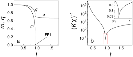
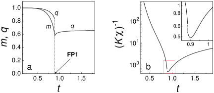
Figure 2: The temperature dependences of $m$, $q$ and inverse static susceptibility $\chi^{-1}$ at $k^{\prime}=2.6$, $d=-10.4$.

Figure 3: The temperature dependences of $m$, $q$ and inverse static susceptibility $\chi^{-1}$ at $k^{\prime}=2.6$, $d=-10.63$.

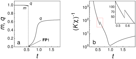
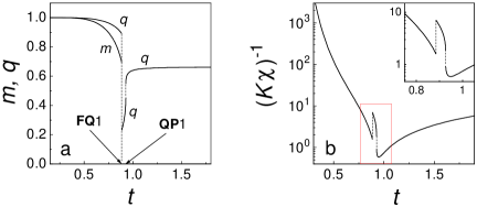
Figure 4: The temperature dependences of $m$, $q$ and inverse static susceptibility $\chi^{-1}$ at $k^{\prime}=2.6$, $d=-10.79$.

Figure 5: The temperature dependences of $m$, $q$ and inverse static susceptibility $\chi^{-1}$ at $k^{\prime}=2.88$, $d=-11.61$.

Figure 6: The temperature dependences of $m$, $q$ and inverse static susceptibility $\chi^{-1}$ at $k^{\prime}=3.44$, $d=-13.34$.

Figure 7: The temperature dependences of $q$ and inverse static susceptibility $\chi^{-1}$ at $k^{\prime}=4.0$, $d=-15.4$.

References

- [1] M. Blume, V.J. Emery, R.B. Griffiths, Phys. Rev. A 4, 1071 (1971).
- [2] D. Mukamel, M. Blume, Phys. Rev. A 10, 610 (1974).
- [3] D. Furman, S. Dattagupta, R.B. Griffiths, Phys. Rev. B 15, 441 (1977).
- [4] J. Sivardiere, Critical and multicritical points in fluids and magnets, Lecture’ Notes in physics. Static critical phenomena in inhomogeneous systems. Proceedings, Karpacz, 1984.
- [5] H.H. Chen, P.M. Levy, Phys. Rev. B 7, 4267 (1973).
- [6] E.L. Nagaev, Magnetics with complicated exchange interaction, Izd. Nauka, Moscow 1988 (In Russian).
- [7] K.E. Newman, J.D. Dow, Phys. Rev. B 27, 7495 (1983).
- [8] T. Iwashita, N. Uryû, Phys. Stat. Sol. (b) 137, 65 (1986).
- [9] R.R. Levitskii, S.I. Sorokov, O.R. Baran, Preprint IFKS-93-1U, Kiev 1993 (In Ukrainian).
- [10] S.I. Sorokov, R.R. Levitskii, O.R. Baran, Ukr. Fiz. Zhurn. 41, 490 (1996) (In Ukrainian).
- [11] S.I. Sorokov, R.R. Levitskii, O.R. Baran, Cond. Mat. Phys. No 9, 57 (1997).
- [12] T. Kaneyoshi, E.F. Sarmento, Physica. A 152, 343 (1988).
- [13] J.W. Tucker, J. Magn. Magn. Mat. 87, 16 (1990).
- [14] K.G. Chakraborty, Phys. Rev. B 29, 1454 (1984).
- [15] A.F. Siqueira, I.P. Fittipaldi, Phys. Stat. Sol. (b) 119, K31 (1983).
- [16] D. Saul, M. Wortis, D. Stauffer, Phys. Rev. B 9, 4964 (1974).
- [17] A. Bakchick, A.Benyoussef, M. Touzani, Physica A 186, 524 (1992).
- [18] O.F. De Alcantara Bonfim, C.H. Obcemea, Z. Phys. B - Condensed Matter 64, 469 (1986).
- [19] R.J.C. Booth, Lu Hua, J.W. Tucker, C.M. Care, I. Halliday, J. Magn. Magn. Mat. 128, 117 (1993).
- [20] K. Kasono, I. Ono, Z. Phys. B - Condensed Matter, 88, 205 (1992).
- [21] D. Pen̂a Lara, J.A. Plascak, International Jornal of Modern Physics. B 12, 2045 (1998).
- [22] B. Strieb, H.B. Callen, Phys. Rev. 130, 1798 (1963).
- [23] V.G. Vaks, Introduction to the microscopic theory of ferroelectrics, Izd. Nauka, Moscow 1973 (In Russian).
- [24] J.S. Smart, Effective field theories of magnetism, Philadelphia-London, W.B.Saunders company, 1996.
- [25] K. Takahashi, M. Tanaka, J. Phys. Soc. Japan 48, 1423 (1980).