Topological Phase Transition Independent of System Non-Hermiticity

Abstract

Non-Hermiticity can vary the topology of system, induce topological phase transition, and even invalidate the conventional bulk-boundary correspondence. Here, we show the introducing of non-Hermiticity without affecting the topological properties of the original chiral symmetric Hermitian systems. Conventional bulk-boundary correspondence holds, topological phase transition and the (non)existence of edge states are unchanged even though the energy bands are inseparable due to non-Hermitian phase transition. Chern number for energy bands of the generalized non-Hermitian system in two dimension is proved to be unchanged and favorably coincides with the simulated topological charge pumping. Our findings provide insights into the interplay between non-Hermiticity and topology. Topological phase transition independent of non-Hermitian phase transition is a unique feature that beneficial for future applications of non-Hermitian topological materials.

Introduction.—Parity-time ($\mathcal{PT}$) symmetry stimulates the development of non-Hermitian physics BenderRPP ; NM ; FL ; EL ; Midya ; YFChen ; Christodoulides ; MANiri . Non-Hermitian systems Ruschhaupt ; ElOL ; BPeng exhibit many intriguing features and applications that not limited to power oscillation Makris ; Ruter , coherent perfect absorption Chong , unidirectionality behaviors Nat ; FLNatMater ; Ramezani14 ; PNAS ; JLPRL , single-mode laser LF ; HH , robust energy transfer Harris ; SFan , and exceptional point (EP) enhanced sensing Wiersig ; ZPLiu ; WChen ; HHodaei due to its nonorthogonal eigenstates and the exotic topology of EPs Heiss01 ; BerryMailybaev ; TGao ; CTChanPRX ; Doppler ; LJin18 . The scope of topological phase of matter has also been extended to non-Hermitian region Rudner ; Szameit11 ; Hughes ; Esaki ; Diehl ; GQLiang ; Malzard ; Kartashov ; YFChenPNAS ; SLieu ; MPan ; HS ; RFleury ; CerjanPRB ; Kunst1812 ; XWLuo18 ; Cancellieri ; YXu19 and stimulates several interesting discussions on $\mathcal{PT}$-symmetric topological interface states OL ; Poli ; Weimann ; Menke ; LJin17 ; PXue ; Yuce ; Ghatak ; KawabataPRB98 ; XNi ; LJLPRB ; SLonghi19 , non-Hermitian bands theory Shen ; Murakami , topological invariants Rakovszky ; Shen ; YXu ; Leykam ; SLin ; WRPRA ; ZXZ19 ; HJiang , EP lines and surfaces BZhen ; ZhouScience ; YXu ; CerjanEPring , semimetals Molina ; Carllstrom ; CHLeeTidal ; Zyuzin ; Schmidt ; JHu ; HZhang , high-order topological phases TLiu ; Ezawa ; JGong ; Edvardsson ; XWLuo , and symmetry protected non-Hermitian topological phases SLin ; Budich ; Yoshida ; Okugawa . Topological classification are discussed for general non-Hermitian systems ZGong ; HZhou ; Kawabata1812 ; KawabataNC , for non-Hermitian systems with reflection symmetry CHLiu , and alteratively classified by the geometric features of singularity ring LinhuLi . The non-Hermiticity and non-Abelian gauge potentials can create interesting topological phases JCai . The robust and efficient topological edge state lasing is an interesting application of non-Hermitian topological systems BBahari ; PStJean ; HZhao ; MParto ; Science ; Kartashov19 .

Topological invariant constructed from the bulk system predicts the topological phase transition and the (non)existence of edge states in the system under open boundary condition Kane , this is referred to as the conventional bulk-boundary correspondence (CBBC). In certain non-Hermitian topological systems, the bulk topology fails to predict the edge states and topological phase transition in systems under open boundary condition TonyPRL ; Martinez ; KawabataPRB ; CHLee ; LJL ; nevertheless, the exotic bulk-boundary correspondences have been reported ZGong ; ZWang ; WYi ; Kunst ; Herviou . A non-Bloch bulk Hamiltonian is constructed to resolve this issue ZWang ; alternatively, topological invariant is established from the biorthogonal edge modes Kunst ; Edvardsson . Furthermore, chiral inversion symmetry is uncovered to protect the CBBC in non-Hermitian topological systems JLBBC , and the CBBC and the skin modes are elucidated in the viewpoint of non-Hermitian Aharonov-Bohm effect; alternatively, they are elucidated from a transfer matrix perspective FKK and the Green’s function method Dan . Besides, the non-Hermiticity can solely induce topological phase, which has been demonstrated in trivial Hermitian systems associated with staggered gain and loss Takata , asymmetric coupling amplitude JLBBC , and imaginary coupling KawabataNC , respectively. Therefore, the non-Hermiticity can alter the topology of system, induce topological phase transition, and even ruin the CBBC; in contrast to the topology changed by non-Hermiticity, retaining the topology of Hermitian system in the non-Hermitian generalization is a critical and meaningful challenge for non-Hermitian topological phase of matter.

In this work, we systematically elucidate the introducing of non-Hermiticity without altering the topological phase transition in the original chiral symmetric Hermitian system; the proposed non-Hermitian topological system holds the CBBC and shares identical topological properties including the (non)existence of topologically protected edge states with their parent Hermitian system, even though the energy bands are deformed into the complex domain and inseparable. The complete set of eigenstates of the non-Hermitian system is exactly mapped from the eigenstates of the original Hermitian system by a set of local transformations; the mapping allows direct projections of their geometric quantities. In the non-Hermitian generalization, five symmetry classes with chiral symmetry are mapped to the other five symmetry classes without chiral symmetry, respectively; the Chern number in two dimension (2D) is proved to be unchanged, and the numerically simulated topological charge pumping favorably agrees with the Chern number.

Mapping the topology.—Chiral symmetric systems can be written in the block off-diagonal form Ryu

$$H=\left(\begin{array}[]{cc}0&D\\ D^{{\dagger}}&0\end{array}\right),$$ (1)

where we consider $D$ as an arbitrary $n\times n$ matrix. The basis in $H$ can be any degree of freedom, such as the real space coordinate, spin, or other orthogonal complete set. $H$ is referred to as the original Hermitian Hamiltonian, from which a non-Hermitian Hamiltonian $\mathcal{H}$ is created

$$\mathcal{H}=H+i\gamma\sigma_{z}\otimes I_{n},$$ (2)

where $\sigma_{z}$ is the Pauli matrix, and $I_{n}$ denotes the $n\times n$ identity matrix. The non-Hermitian term $i\gamma$ in $\mathcal{H}$ does not only play the role of on-site potential, but also the non-Hermitian hopping with asymmetric amplitudes in the real space. For chiral symmetric systems not in the bipartite lattice form, taken the Creutz ladder as an illustration TonyPRL , the gain and loss introduced in the block off-diagonal form of $H$ [Eq. (1)] are equivalent to introducing asymmetric couplings in the ladder legs JLBBC . In addition, introducing non-Hermiticity breaks the chiral symmetry.

Equation (2) provides a way of non-Hermitian generalization without altering the topological phase transition in original Hermitian systems. To characterize the topological properties, we consider the Hamiltonian $H(\mathbf{k)}$ in the momentum space, which is the core matrix of a Bloch or a BdG system Ryu . $\mathbf{k}$ is the momentum and all the information of the topological system is encoded in $H(\mathbf{k)}$. The Schrödinger equation is $H(\mathbf{k})\left|\phi_{\lambda}^{\rho}(\mathbf{k})\right\rangle=\varepsilon_{\lambda}^{\rho}(\mathbf{k})\left|\phi_{\lambda}^{\rho}(\mathbf{k})\right\rangle$ and $\mathcal{H}(\mathbf{k})\left|\varphi_{\lambda}^{\rho}(\mathbf{k})\right\rangle=\epsilon_{\lambda}^{\rho}(\mathbf{k})\left|\varphi_{\lambda}^{\rho}(\mathbf{k})\right\rangle$, where $\rho=\pm$ represents the upper or lower energy band, and $\lambda\in[1,l]$ denotes the band index, assuming the total number of energy bands $2l$. The eigenenergy of $\mathcal{H}(\mathbf{k})$ is

$$\epsilon_{\lambda}^{\rho}\left(\mathbf{k}\right)=\rho[\varepsilon_{\lambda}^{\rho}\left(\mathbf{k}\right)^{2}-\gamma^{2}]^{1/2}.$$ (3)

The energy is either real or imaginary. The eigenstate of $\mathcal{H}(\mathbf{k})$ for eigenenergy $\epsilon_{\lambda}^{\rho}(\mathbf{k})$ is obtained through a mapping (see Appendix A)

$$\left|\varphi_{\lambda}^{\rho}(\mathbf{k})\right\rangle=M_{\lambda}^{\rho}(\mathbf{k},\gamma)\left|\phi_{\lambda}^{\rho}(\mathbf{k})\right\rangle.$$ (4)

with the mapping matrix

$$M_{\lambda}^{\rho}(\mathbf{k},\gamma)=\left(\begin{array}[]{cc}a_{\lambda}^{\rho}\left(\mathbf{k},\gamma\right)I_{n}&0\\ 0&I_{n}\end{array}\right),$$ (5)

where $a_{\lambda}^{\rho}\left(\mathbf{k},\gamma\right)=[\epsilon_{\lambda}^{\rho}(\mathbf{k})+i\gamma]/\varepsilon_{\lambda}^{\rho}(\mathbf{k})$ is a unit modulus complex number for real $\epsilon_{\lambda}^{\rho}\left(\mathbf{k}\right)$, and $\left|a_{\lambda}^{\rho}\left(\mathbf{k},\gamma\right)\right|\neq 1$ for imaginary $\epsilon_{\lambda}^{\rho}\left(\mathbf{k}\right)$. The mapping $M_{\lambda}^{\rho}(\mathbf{k,}\gamma)$ acts as a local transformation, which is essential for the inheritance of topological features from the original Hermitian system in the non-Hermitian generalization.

Bulk-boundary correspondence.—CBBC does not always hold in non-Hermitian topological systems TonyPRL ; Martinez ; ZGong ; ZWang ; WYi ; LJL , where effective imaginary gauge field induces a non-Hermitian Aharonov-Bohm effect that invalidates the CBBC CHLee ; JHu ; ZWang ; JLBBC . Considering a bipartite lattice Hamiltonian Lieb , the gain and loss are respectively introduced in two sublattices for the proposed manner [Eq. (2)]. $\mathcal{H}$ is a $2n$-site non-Hermitian lattice constituted by $n$ coupled $\mathcal{PT}$-symmetric dimers. Applying a unitary transformation, the intra dimer coupling $J$ associated with the gain and loss $\gamma$ in a $\mathcal{PT}$-symmetric dimer changes into the asymmetric intra dimer couplings $J\pm\gamma$ (see Appendix B), which appears as inter sublattice couplings; and the effective imaginary gauge field is absent along the translational invariant direction of the sublattice, the non-Hermitian Aharonov-Bohm effect does not occur, and the CBBC holds.

Alternatively, the validity of CBBC can be straightforwardly understood from the mapping between the original Hermitian topological system and the generalized non-Hermitian topological system. Although the energy bands are tightened [Eq. (3)] after introduced the non-Hermiticity, the band structures and their topologies are unchanged. The mapping matrix [Eq. (5)] retains the profile of the eigenstates; the Dirac probability distribution of the eigenstates inside each sublattice is unchanged after mapping [Eq. (4)]. The CBBC is valid for the non-Hermitian system $\mathcal{H}$ and does not require the symmetry protection, this differs from that in Ref. JLBBC .

Mapping of symmetry classes.—In the ten Altland-Zirnbauer classes AZ , topological systems with chiral symmetry include five symmetry classes and satisfy $\mathcal{S}H(\mathbf{k)}\mathcal{S}^{-1}=-H(\mathbf{k)}$ Ryu , where the chiral operator is $\mathcal{S}=\sigma_{z}\otimes I_{n}\mathcal{=S}^{-1}$. The symmetry class $\mathrm{AIII}$ does not have additional discrete symmetries, only a combined time-reversal ($\mathcal{T}$) and particle-hole ($\mathcal{C}$) symmetry $\mathcal{S}=\mathcal{TC}$ is present. The symmetry classes $\mathrm{BDI}$, $\mathrm{CII}$, $\mathrm{CI}$, and $\mathrm{DIII}$ have additional time-reversal and particle-hole symmetries under $\mathcal{T}H(-\mathbf{k})\mathcal{T}^{-1}=H(\mathbf{k)}$ and $\mathcal{C}H(-\mathbf{k)}\mathcal{C}^{-1}=-H(\mathbf{k)}$. After introducing the non-Hermiticity, the chiral symmetry vanishes in non-Hermitian topological systems $\mathcal{H(}\mathbf{k)}=H\mathcal{(}\mathbf{k)}+i\gamma\sigma_{z}\otimes I_{n}$.

From $\mathcal{S}=\mathcal{TC}$, we obtain $\mathcal{T}^{-1}=\mathcal{CS}^{-1}=\mathcal{CS}$. Then we have $\mathcal{T}\left(i\gamma\mathcal{S}\right)\mathcal{T}^{-1}=-i\gamma\mathcal{T}\left(\mathcal{TC}\right)\left(\mathcal{CS}\right)=-i\gamma\mathcal{T}^{2}\mathcal{C}^{2}\mathcal{\mathcal{S}}$. From $\mathcal{T}=\mathcal{SC}^{-1}$, we obtain $\mathcal{C}\left(i\gamma\mathcal{S}\right)\mathcal{C}^{-1}=-i\gamma\mathcal{CT}^{2}\mathcal{\mathcal{T}}^{-1}=-i\gamma\mathcal{T}^{2}\mathcal{C}\left(\mathcal{C\mathcal{S}}\right)=-i\gamma\mathcal{T}^{2}\mathcal{C}^{2}\mathcal{\mathcal{S}}$. Thus under the action of time-reversal and particle-hole operators, the non-Hermitian term $i\gamma(\sigma_{z}\otimes I_{n})=i\gamma\mathcal{S}$ satisfies

$$\mathcal{T}(i\gamma\mathcal{S})\mathcal{T}^{-1}=\mathcal{C}(i\gamma\mathcal{S})\mathcal{C}^{-1}=-i\gamma\mathcal{T}^{2}\mathcal{\mathcal{C}}^{2}\mathcal{S}.$$ (6)

After the non-Hermitian generalization, the symmetry class $\mathrm{AIII}$ $H\mathcal{(}\mathbf{k)}$ changes to symmetry class $\mathrm{A}$ $\mathcal{H(}\mathbf{k)}$. The chiral orthogonal ($\mathrm{BDI)}$ class has $\mathcal{T}^{2}\mathcal{\mathcal{C}}^{2}\mathcal{S}=\left(+1\right)\left(+1\right)\mathcal{S}$. Thus,

$$\mathcal{TH(}\mathbf{k)}\mathcal{T}^{-1}=H(-\mathbf{k)}-i\gamma(\sigma_{z}\otimes I_{n})\neq\mathcal{H}(-\mathbf{k),}$$ (7)

but

$$\mathcal{CH}\mathbf{(k)}\mathcal{C}^{-1}=-H(-\mathbf{k)}-i\gamma(\sigma_{z}\otimes I_{n})=-\mathcal{H}(-\mathbf{k}).$$ (8)

The time-reversal symmetry breaks, but the particle-hole symmetry holds for the non-Hermitian topological systems; the symmetry class $\mathrm{BDI}$ is mapped to the symmetry class $\mathrm{D}$. The chiral symplectic ($\mathrm{CII}$) class has $\mathcal{T}^{2}\mathcal{\mathcal{C}}^{2}\mathcal{S}=\left(-1\right)\left(-1\right)\mathcal{S}$; similarly, only the particle-hole symmetry holds $\mathcal{CH}(-\mathbf{k})\mathcal{C}^{-1}=-\mathcal{H}\mathbf{(k})$ and the symmetry class $\mathrm{CII}$ is mapped to the symmetry class $\mathrm{C}$. For the other two symmetry classes with chiral symmetry, the symmetry class $\mathrm{CI}$ has $\mathcal{T}^{2}\mathcal{\mathcal{C}}^{2}\mathcal{S}=\left(+1\right)\left(-1\right)\mathcal{S}$ and the symmetry class $\mathrm{DIII}$ has $\mathcal{T}^{2}\mathcal{\mathcal{C}}^{2}\mathcal{S}=\left(-1\right)\left(+1\right)\mathcal{S}$; both two classes satisfy

$$\mathcal{TH}\mathbf{(k)}\mathcal{T}^{-1}=H(-\mathbf{k)}+i\gamma(\sigma_{z}\otimes I_{n})=\mathcal{H}(-\mathbf{k),}$$ (9)

but

$$\mathcal{CH}(\mathbf{k)}\mathcal{C}^{-1}=-H(-\mathbf{k)}+i\gamma(\sigma_{z}\otimes I_{n})\neq-\mathcal{H}(-\mathbf{k).}$$ (10)

The time-reversal symmetry holds, but the particle-hole symmetry breaks in the non-Hermitian generalization. The mappings of symmetry classes are $\mathrm{CI}\rightarrow\mathrm{AI}$ and $\mathrm{DIII}\rightarrow\mathrm{AII}$. In summary, the introduced non-Hermiticity breaks the chiral symmetry and one of the time-reversal and particle-hole symmetries; the five symmetry classes with chiral symmetry shift to the other five symmetry classes without chiral symmetry

$$\mathrm{AIII\rightarrow A,BDI\rightarrow D,CII\rightarrow C,CI\rightarrow AI,DIII\rightarrow AII.}$$ (11)

Chern number in 2D systems.—Considering a 2D topological system, the (first) Chern numbers for each band of the two Hamiltonians $H(\mathbf{k})$ and $\mathcal{H}(\mathbf{k})$ are exactly identical. In the absence of EPs, the energy bands are separable, the four types of Chern numbers defined under the right and left eigenstates of $\mathcal{H}(\mathbf{k})$ are identical Shen ; YXu19 (see Appendix C). For separable bands of the Hermitian Hamiltonian, the bands of non-Hermitian Hamiltonian are “separable” in practice even if the energy bands merge in the presence of EPs. To see that the Chern number is a topological invariant and does not change in the mapping, we employ the conventional definition; unlike the lack of biorthonormal basis at EPs Ali02 , whose biorthonormal probability vanishes at the exceptional point $\mathbf{k}$ for certain bands, the Berry connections $\mathbf{A}_{\lambda}^{\rho}=i\left\langle\phi_{\lambda}^{\rho}(\mathbf{k})\right|\nabla_{\mathbf{k}}\left|\phi_{\lambda}^{\rho}(\mathbf{k})\right\rangle$ for $H(\mathbf{k})$ and $\overrightarrow{\mathcal{A}}_{\lambda}^{\rho}=i\left\langle\varphi_{\lambda}^{\rho}(\mathbf{k})\right|\nabla_{\mathbf{k}}\left|\varphi_{\lambda}^{\rho}(\mathbf{k})\right\rangle$ for $\mathcal{H}(\mathbf{k})$ based on the right eigenstates are always well-defined. The nabla operator is $\nabla_{\mathbf{k}}=(\partial_{k_{x}},\partial_{k_{y}})$.

Direct derivation yields $\overrightarrow{\mathcal{A}}_{\lambda}^{\rho}=\mathbf{A}_{\lambda}^{\rho}-\left(1/2\right)\nabla_{\mathbf{k}}\vartheta$ [$\overrightarrow{\mathcal{A}}_{\lambda}^{\rho}=\mathbf{A}_{\lambda}^{\rho}+$ $\left\langle\phi_{\lambda}^{-\rho}(\mathbf{k})\right|i\nabla_{\mathbf{k}}\left|\phi_{\lambda}^{\rho}(\mathbf{k})\right\rangle\epsilon_{\lambda}^{\rho}(\mathbf{k})/\left(i\gamma\right)$] for real (imaginary) spectrum, in which $\vartheta=\arctan[\gamma/\epsilon_{\lambda}^{\rho}(\mathbf{k})]$; the relation is gauge dependent (see Appendix C), however, the Berry curvatures are gauge independent $\mathbf{B}_{\lambda}^{\rho}=\nabla_{\mathbf{k}}\times\mathbf{A}_{\lambda}^{\rho}$, $\overrightarrow{\mathcal{B}}_{\lambda}^{\rho}=\nabla_{\mathbf{k}}\times\overrightarrow{\mathcal{A}}_{\lambda}^{\rho}$, and obey $\mathbf{B}_{\lambda}^{\rho}=\overrightarrow{\mathcal{B}}_{\lambda}^{\rho}$ ($\mathbf{B}_{\lambda}^{\rho}\neq\overrightarrow{\mathcal{B}}_{\lambda}^{\rho}$) for real (imaginary) spectrum; and the contribution of the later term in $\overrightarrow{\mathcal{A}}_{\lambda}^{\rho}$ for the Chern number $c_{\lambda}^{\rho}$ is zero,

$$c_{\lambda}^{\rho}=\frac{1}{2\pi}\oint\mathbf{B}_{\lambda}^{\rho}d^{2}\mathbf{k=}\frac{1}{2\pi}\oint\overrightarrow{\mathcal{B}}_{\lambda}^{\rho}d^{2}\mathbf{k.}$$ (12)

This is referred to as the topological invariant mapping. Notably, the mapping Eq. (4) is directly applicable to the edge states. These conclusions are not relevant to the reality of energy bands and the presence of EPs. The Chern numbers for each energy band of both systems are identical even if the bands merge in the presence of EPs (see Appendix C).

Ultracold atomic gases Goldman ; Cooper , acoustic lattices RF ; YFChenNP , electrical circuits EzawaPRB ; RYu ; CHLeeCP , and various microwave, optical, and photonic systems Hafezi ; LLu ; Ozawa have became fertile platforms for studying topological phase of matter. Through introducing additional losses, passive non-Hermitian topological systems are created CerjanEPring ; ZhouScience ; the properties of $\mathcal{PT}$-symmetric systems with balanced gain and loss are exacted from the passive systems by shifting a common loss rate. Nowadays, the non-Hermitian topological systems are experimentally realized via sticking absorbers in the dielectric resonator array Poli , cutting the waveguides in coupled optical waveguide lattice CerjanEPring , and fabricating the radiative loss in open systems of photonic crystals Weimann ; ZhouScience . Active elements are required to realize robust topological edge state lasing BBahari ; Science ; HZhao ; PStJean ; MParto ; Kartashov19 , where external pumping is implemented to acquire the gain. The prototypical non-Hermitian topological system is the 1D complex Su–Schrieffer–Heeger (SSH) model OL ; here we consider a simple extension to interpret the Chern number in the non-Hermitian generalization from the viewpoint of topological charge pumping. Figure 1(a) shows the 1D comb lattice formed via staggered side-coupled additional sites to the intensively investigated complex SSH lattice in experiment Poli ; Weimann ; MPan ; MParto ; PStJean ; HZhao ; YDChong18 .

Topological charge pumping.—In the momentum space, the core matrix is

$$H\left(k\right)=\left(\begin{array}[]{cccc}0&0&\mu_{k}&\kappa_{+}\\ 0&0&\kappa_{-}&0\\ \mu_{-k}&\kappa_{-}&0&0\\ \kappa_{+}&0&0&0\end{array}\right),$$ (13)

where $\mu_{k}=J(1-\delta)+J(1+\delta)e^{ik}$ and the system parameters are $\delta=\delta_{0}+R\cos\theta$ and $\kappa_{\pm}=\kappa_{0}\pm(1/2)R\sin\theta$ (set $\kappa\equiv\kappa_{+}-\kappa_{-}=R\sin\theta$), forming a loop $L$ with radius $R$($>0$) in the parameter space. The core matrix of the non-Hermitian generalization $\mathcal{H}\left(k\right)$ gives

$$\mathcal{H}(k)=H(k)+i\gamma\sigma_{z}\otimes I_{2}.$$ (14)

$H(k)$ belongs to symmetry class BDI, and $\mathcal{H}(k)$ belongs to symmetry class D only with the particle-hole symmetry, $\mathcal{CH}(k)\mathcal{C}^{-1}=-\mathcal{H}(-k)$, where $\mathcal{C}=\left(\sigma_{z}\otimes I_{2}\right)\mathcal{K}$, $I_{2}$ is the $2\times 2$ identity matrix, and $\mathcal{K}$ is the complex conjugation. Eigenstates $\{|\varphi_{\lambda}^{\rho}(k)\rangle,|\eta_{\lambda}^{\rho}(k)\rangle\}$ for $\{\mathcal{H}(k),\mathcal{H}^{\dagger}(k)\}$ are obtained from the eigenstates of $H(k)$ through mapping (see Appendix D). The corresponding energy for eigenstate $\left|\varphi_{\lambda}^{\rho}(k)\right\rangle$ is $\epsilon_{\lambda}^{\rho}=\rho[\Upsilon_{k}+\lambda(\Upsilon_{k}^{2}-\kappa_{+}^{2}\kappa_{-}^{2})^{1/2}-\gamma^{2}]^{1/2}$ with $\Upsilon_{k}=(\left|\mu_{k}\right|^{2}+\kappa_{+}^{2}+\kappa_{-}^{2})/2$ and $\rho,\lambda=\pm$.

For nonzero $\kappa_{+}\kappa_{-}$ in Hermitian $H(k)$, this four-band model can be regarded as two identical Rice-Mele models WRPRB . The topological features of the Rice-Mele model retain in the non-Hermitian generalization. The Chern number $c_{\lambda}^{\rho}$ has a precise physical meaning: the quantum particle transport for the energy band $(\rho,\lambda)$ over an enclosed adiabatic passage along a closed cycle XiaoDRMP . $c_{\lambda}^{\rho}$ equals to the winding number of loop around the band touching point $\left(\delta,\kappa\right)=\left(0,0\right)$ in the parameter space.

The biorthonormal current Book ; KawabataPRB98 across sites $a_{N}$ and $b_{N-1}$ is

$$j_{N}(t)=-i\sum_{m=1}^{N}\langle\eta_{m}(t)|\{J[1-\delta(t)]a_{N}^{\dagger}b_{N-1}-\mathrm{H.c.}\}|\varphi_{m}(t)\rangle,$$ (15)

where $m$ is the number of energy levels in the concerned energy band for the $4N$ size system with periodic boundary condition. The parameters vary as $\theta=\omega t$ in the numerical simulation under a quasi-adiabatic process, where the speed of time evolution $\omega\ll 1$, and $t$ varies from $0$ to a period of $T=2\pi\omega^{-1}$. To demonstrate a quasi-adiabatic process, we keep $f\left(t\right)=\left|\langle\bar{\eta}_{m}(t)\left|\varphi_{m}(t)\right\rangle\right|\rightarrow 1$ during the whole process by taking sufficient small $\omega$, where $\left|\bar{\eta}_{m}\left(t\right)\right\rangle$ is the corresponding instantaneous eigenstate of $\mathcal{H}^{\dagger}\left(t\right)$. For the given initial eigenstates $|\varphi_{m}(0)\rangle=|\varphi_{-,m}^{-}\rangle$ and $|\eta_{m}(0)\rangle=|\eta_{-,m}^{-}\rangle$, the time evolved states are $\left|\varphi_{m}(t)\right\rangle=$ $\mathcal{T}_{t}\exp[-i\int_{0}^{t}\mathcal{H}(t^{\prime})\mathrm{d}t^{\prime}]\left|\varphi_{m}(0)\right\rangle$ and $\left|\eta_{m}(t)\right\rangle=$ $\mathcal{T}_{t}\exp[-i\int_{0}^{t}\mathcal{H}^{\dagger}(t^{\prime})\mathrm{d}t^{\prime}]\left|\eta_{m}(0)\right\rangle$, where $\mathcal{T}_{t}$ is the time ordering operator and $\mathcal{H}\left(t\right)$ is the Hamiltonian in the real space. The accumulated charge pumping WRPRA ; WRPRB passing the dimer $a_{N}b_{N-1}$ during the interval $t$ is

$$Q_{N}(t)=\int_{0}^{t}j_{N}(t^{\prime})dt^{\prime}.$$ (16)

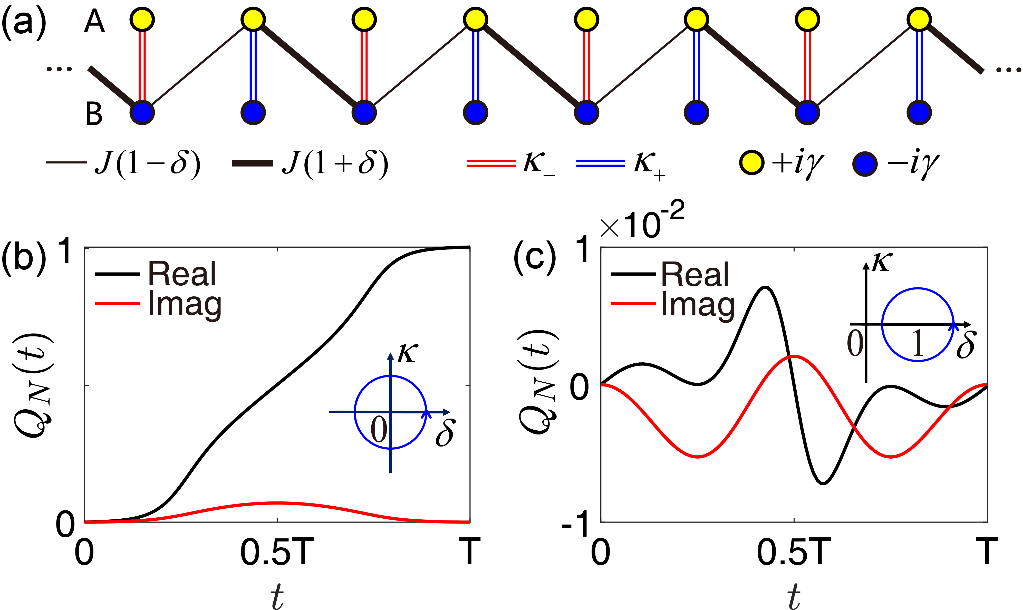
Figure 1: (a) Schematic of the comb lattice. Numerical simulations of $Q_{N}(t)$ for the band $(\rho,\lambda)=(-,-)$ in two quasi-adiabatic processes (insets) of (b) $\delta_{0}=0$ and (c) $\delta_{0}=1$ at $\gamma=0.5$, $\omega=10^{-3}$, and $T=2\pi/\omega$. Real (imaginary) part of $Q_{N}(t)$ is in black (red); the corresponding $j_{N}(t)$ is shown in Appendix E.

The topological charge pumping favorably agrees with the Chern number $c_{-}^{-}=1$ [Fig. 1(b)] in the nontrivial phase or $c_{-}^{-}=0$ [Fig. 1(c)] in the trivial phase for real energy band as that in the Hermitian topological systems Thouless ; Kraus ; XDai . For imaginary energy band without EPs, the amplitude of evolved states $\left|\eta_{m}(t)\right\rangle$ and $\left|\varphi_{m}(t)\right\rangle$ exponentially increase (or decrease); performing the quantization of transport in a counterpart Hamiltonian $\mathcal{H}^{\prime}(k)=i\mathcal{H}(k)$ with corresponding real energy band is feasible to verify the Chern number and the topological properties of imaginary energy band of $\mathcal{H}(k)$, since $\mathcal{H}^{\prime}(k)$ has identical topology and eigenstate with $\mathcal{H}(k)$.

Alternatively, the topological charge pumping can be retrieved from the dynamical evolution of edge states in the edge Hamiltonian $\mathcal{H}_{\mathrm{edge}}$ (see Appendix E), which is generated by truncating a coupling $J(1+\delta)$ at the lattice boundary of the bulk Hamiltonian $\mathcal{H}$ in the real space [Fig. 1(a)]. $\mathcal{H}_{\mathrm{edge}}$ and $H_{\mathrm{edge}}$ meet the condition of mapping since Eq. (2) still holds. Two pairs of edge states exist

$$|\varphi_{\mathrm{R}}^{\pm}\rangle = \frac{1}{\sqrt{\Omega}}\sum\limits_{j=1}^{N}\varsigma^{N-j}(e^{\pm i\vartheta_{\mathrm{R}}}a_{2j}^{\dagger}\pm b_{2j}^{\dagger})\left|\mathrm{vac}\right\rangle,$$ (17)

$$|\varphi_{\mathrm{L}}^{\pm}\rangle = \frac{1}{\sqrt{\Omega}}\sum\limits_{j=1}^{N}\varsigma^{j-1}(e^{\pm i\vartheta_{\mathrm{L}}}a_{2j-1}^{\dagger}\pm b_{2j-1}^{\dagger})\left|\mathrm{vac}\right\rangle,$$ (18)

associated with the energies $\epsilon_{\mathrm{R}}^{\pm}=\pm(\kappa_{+}^{2}-\gamma^{2})^{1/2}$ and $\epsilon_{\mathrm{L}}^{\pm}=\pm(\kappa_{-}^{2}-\gamma^{2})^{1/2}$, respectively; where $\varsigma=(\delta-1)/(\delta+1)$, $\Omega=2(1-\varsigma^{2N})/(1-\varsigma^{2})$, $e^{\pm i\vartheta_{\mathrm{R}}}=(\epsilon_{\mathrm{R}}^{+}\pm i\gamma)/\kappa_{+}$ and $e^{\pm i\vartheta_{\mathrm{L}}}=(\epsilon_{\mathrm{L}}^{+}\pm i\gamma)/\kappa_{-}$. The explicit expressions of edge states reveal a fact that the mapping matrix only changes the local phase or amplitude. For real $\epsilon_{\mathrm{R/L}}^{\pm}$, the edge state profiles are independent of $\gamma$ and $\kappa_{\pm}$ similar as that in Hermitian XiaoDRMP and non-Hermitian WRPRA Rice-Mele models; for imaginary $\epsilon_{\mathrm{R/L}}^{\pm}$, the probability becomes dense in the sublattice with gain (loss) for $|\varphi_{\mathrm{R/L}}^{+}\rangle$ ($|\varphi_{\mathrm{R/L}}^{-}\rangle$) BPeng . The topological charge pumping of an edge state for a loop $L$ in the $\kappa$-$\delta$ plane equals to the Chern number Hatsugai (see Appendix E). The energy bands are gapped and real at $\gamma=0$; as $\gamma$ increasing, imaginary energy levels appear and non-Hermitian phase transition occurs. In Figs. 2(a) and 2(b), the energy bands are depicted at weak and strong $\gamma$, respectively. The not shown imaginary part for real band is zero and vice versa. The edge states retain although energy bands become imaginary. Recently, we notice an experimental work that reported the existence of topological edge states in both unbroken and broken $\mathcal{PT}$-symmetric phases PXue1906 .

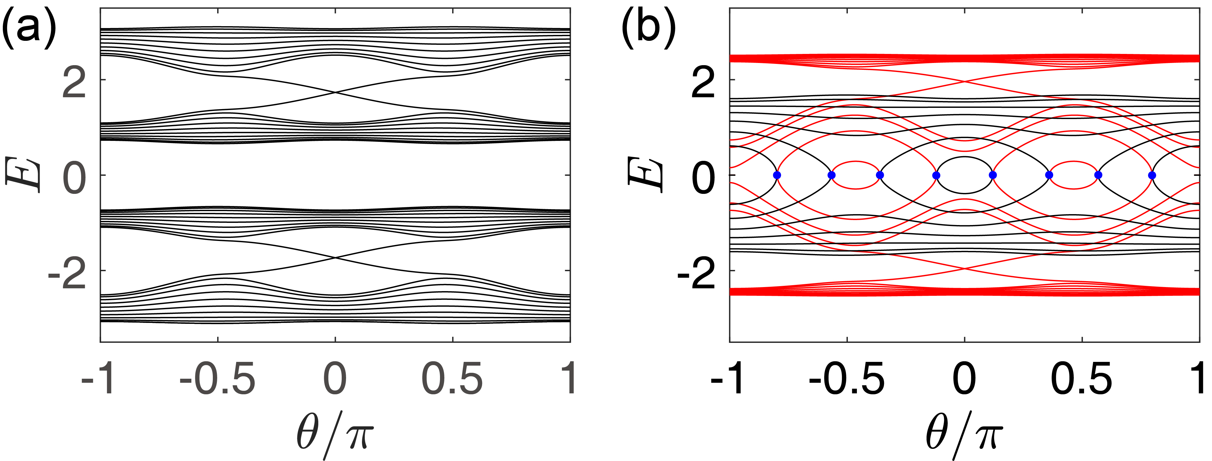
Figure 2: Energy bands of the edge Hamiltonian for $\delta_{0}=0$ at (a) $\gamma=1.0$ and (b) $\gamma=2.8$, the real (imaginary) part is in black (red), the blue dots are EPs. Other parameters are $J=1$, $\kappa_{0}=2$, $R=0.6$, and $N=10$.

Discussion and conclusion.—For chiral symmetric systems not in the form of a bipartite lattice TonyPRL , we can first apply a unitary transformation to get the block off-diagonal form Hamiltonian [Eq. (1)]; then, introduce the non-Hermiticity [Eq. (2)]; after the inversion unitary transformation, a non-Hermitian system possessing identical topology to the chiral symmetric Hermitian system is generated. Notably, the mapping theory is applicable for $H\mathbf{(q)}$ instead of the core matrix $H\mathbf{(k)}$, where $\mathbf{q}$ is a set of periodic parameters instead of the momentum $\mathbf{k}$. In addition to the gapped topological systems, the non-Hermitian generalizations are applicable for gapless topological systems MPan ; OZ ; Lieu ; SLin17 ; ZKLSR ; WPSR . After introducing the non-Hermiticity in the proposed manner, the gapless degeneracy points may change into pairs of EPs, EP rings, or EP surfaces Weimann ; Szameit11 ; CerjanPRB ; CerjanEPring ; although the non-Hermitian phase transition occurs, the topology remains unchanged and can be characterized by winding number as indicated in Refs. YXu ; YXu19 ; CerjanPRB .

Our findings provide insights into the interplay between non-Hermiticity and topology. In contrast to the topological phase transition induced by the non-Hermiticity, we propose the non-Hermitian generalization that completely retains the topological phase transition and the (non)existence of edge states in the original chiral symmetric Hermitian systems; and the non-Hermitian phase transition does not alter or destroy the original topology. This dramatically differs from the non-Hermiticity induced topological phase transition Takata ; KawabataNC , differs from the breakdown of CBBC induced by gain and loss or non-Hermitian asymmetric coupling TonyPRL ; Martinez ; KawabataPRB ; HZhang ; CHLee ; LJL ; ZGong ; ZWang ; WYi ; Kunst ; and differs from the situation that the strong non-Hermiticity destroys the topological edge states due to the non-Hermitian phase transition associated with the appearance of band touching EPs JLBBC . The topological phase transition and the non-Hermitian phase transition are independent and separately controllable. This unique feature is valuable for the explorations of novel non-Hermitian topological phases and topologically protected edge state lasing.

Acknowledgment.—This work was supported by National Natural Science Foundation of China (Grants No. 11874225 and No. 11605094).

Appendix

A Mapping matrix

The Schrödinger equation for the original Hermitian Hamiltonian $H(\mathbf{k})$ is $H(\mathbf{k})\left|\phi_{\lambda}^{\rho}(\mathbf{k})\right\rangle=\varepsilon_{\lambda}^{\rho}(\mathbf{k})\left|\phi_{\lambda}^{\rho}(\mathbf{k})\right\rangle$. $H(\mathbf{k})$ is the parent Hamiltonian in the non-Hermitian generalization, and has the chiral symmetry,

$$H(\mathbf{k})=\left(\begin{array}[]{cc}0&D(\mathbf{k})\\ D^{\dagger}(\mathbf{k})&0\end{array}\right),$$ (A1)

where we consider $D(\mathbf{k})$ as an arbitrary $n\times n$ matrix.

The eigenstates of $\mathcal{H}(\mathbf{k})=H(\mathbf{k})+i\gamma\left(\sigma_{z}\otimes I_{n}\right)$ are

$$\left|\varphi_{\lambda}^{\rho}(\mathbf{k})\right\rangle=M_{\lambda}^{\rho}\left(\mathbf{k,}\gamma\right)\left|\phi_{\lambda}^{\rho}(\mathbf{k})\right\rangle,$$ (A2)

with eigenvalues

$$\epsilon_{\lambda}^{\rho}(\mathbf{k})=\rho\sqrt{\left[\varepsilon_{\lambda}^{\rho}\left(\mathbf{k}\right)\right]^{2}-\gamma^{2}},$$ (A3)

where the mapping matrix has the form

$$M_{\lambda}^{\rho}\left(\mathbf{k,}\gamma\right)=\left(\begin{array}[]{cc}a_{\lambda}^{\rho}\left(\mathbf{k,}\gamma\right)I_{n}&0\\ 0&I_{n}\end{array}\right),$$ (A4)

and $a_{\lambda}^{\rho}\left(\mathbf{k,}\gamma\right)=\left[\epsilon_{\lambda}^{\rho}\left(\mathbf{k}\right)+i\gamma\right]/\varepsilon_{\lambda}^{\rho}\left(\mathbf{k}\right)$ fulfills $\left|a_{\lambda}^{\rho}\left(\mathbf{k,}\gamma\right)\right|=1$ for real $\epsilon_{\lambda}^{\rho}\left(\mathbf{k}\right)$ and is pure imaginary for imaginary $\epsilon_{\lambda}^{\rho}\left(\mathbf{k}\right)$. For real $\epsilon_{\lambda}^{\rho}\left(\mathbf{k}\right)$, the factor $a_{\lambda}^{\rho}\left(\mathbf{k,}\gamma\right)$ can be written in the form of $a_{\lambda}^{\rho}\left(\mathbf{k,}\gamma\right)=e^{i\vartheta}$, with $\vartheta=\arctan\left[\gamma/\epsilon_{\lambda}^{\rho}\left(\mathbf{k}\right)\right]$.

Notice that,

$$H\left(\mathbf{k}\right)M_{\lambda}^{\rho}\left(\mathbf{k,}\gamma\right)=\left(\begin{array}[]{cc}I_{n}&0\\ 0&a_{\lambda}^{\rho}\left(\mathbf{k,}\gamma\right)I_{n}\end{array}\right)H\left(\mathbf{k}\right),$$ (A5)

we have $H\left(\mathbf{k}\right)\left|\varphi_{\lambda}^{\rho}\left(\mathbf{k}\right)\right\rangle=\left[H\left(\mathbf{k}\right)M_{\lambda}^{\rho}\left(\mathbf{k,}\gamma\right)\right]\left|\phi_{\lambda}^{\rho}\left(\mathbf{k}\right)\right\rangle$, then,

$$H\left(\mathbf{k}\right)\left|\varphi_{\lambda}^{\rho}\left(\mathbf{k}\right)\right\rangle$$ (A8)

$$= \varepsilon_{\lambda}^{\rho}\left(\mathbf{k}\right)\left(\begin{array}[]{cc}I_{n}&0\\ 0&a_{\lambda}^{\rho}\left(\mathbf{k,}\gamma\right)I_{n}\end{array}\right)\left|\phi_{\lambda}^{\rho}\left(\mathbf{k}\right)\right\rangle$$

$$= \varepsilon_{\lambda}^{\rho}\left(\mathbf{k}\right)\left(\begin{array}[]{cc}\left[a_{\lambda}^{\rho}\left(\mathbf{k,}\gamma\right)\right]^{-1}I_{n}&0\\ 0&a_{\lambda}^{\rho}\left(\mathbf{k,}\gamma\right)I_{n}\end{array}\right)\left|\varphi_{\lambda}^{\rho}\left(\mathbf{k}\right)\right\rangle,$$ (A11)

therefore, we obtain

$$\mathcal{H}\left(\mathbf{k}\right)\left|\varphi_{\lambda}^{\rho}\left(\mathbf{k}\right)\right\rangle = \left[H\left(\mathbf{k}\right)+i\gamma\sigma_{z}\otimes I_{n}\right]\left|\varphi_{\lambda}^{\rho}\left(\mathbf{k}\right)\right\rangle$$ (A14)

$$= \left(\begin{array}[]{cc}\{\varepsilon_{\lambda}^{\rho}\left(\mathbf{k}\right)\left[a_{\lambda}^{\rho}\left(\mathbf{k,}\gamma\right)\right]^{-1}+i\gamma\}I_{n}&0\\ 0&\left[\varepsilon_{\lambda}^{\rho}\left(\mathbf{k}\right)a_{\lambda}^{\rho}\left(\mathbf{k,}\gamma\right)-i\gamma\right]I_{n}\end{array}\right)\left|\varphi_{\lambda}^{\rho}\left(\mathbf{k}\right)\right\rangle.$$

From $a_{\lambda}^{\rho}\left(\mathbf{k,}\gamma\right)=\left[\epsilon_{\lambda}^{\rho}\left(\mathbf{k}\right)+i\gamma\right]/\varepsilon_{\lambda}^{\rho}\left(\mathbf{k}\right)$ and $\epsilon_{\lambda}^{\rho}(\mathbf{k})=\rho\sqrt{\left[\varepsilon_{\lambda}^{\rho}\left(\mathbf{k}\right)\right]^{2}-\gamma^{2}}$, we have $\varepsilon_{\lambda}^{\rho}\left(\mathbf{k}\right)\left[a_{\lambda}^{\rho}\left(\mathbf{k,}\gamma\right)\right]^{-1}+i\gamma=\varepsilon_{\lambda}^{\rho}\left(\mathbf{k}\right)a_{\lambda}^{\rho}\left(\mathbf{k,}\gamma\right)-i\gamma=\epsilon_{\lambda}^{\rho}\left(\mathbf{k}\right)$. Thus,

$$\mathcal{H}\left(\mathbf{k}\right)\left|\varphi_{\lambda}^{\rho}\left(\mathbf{k}\right)\right\rangle=\epsilon_{\lambda}^{\rho}\left(\mathbf{k}\right)\left|\varphi_{\lambda}^{\rho}\left(\mathbf{k}\right)\right\rangle.$$ (A15)

In parallel, the eigenstate of $\mathcal{H}^{\dagger}\left(\mathbf{k}\right)$ is given by $\left|\eta_{\lambda}^{\rho}\left(\mathbf{k}\right)\right\rangle=\left[M_{\lambda}^{\rho}\left(\mathbf{k,}\gamma\right)\right]^{\dagger}\left|\phi_{\lambda}^{\rho}\left(\mathbf{k}\right)\right\rangle$ with eigenvalue $\left[\epsilon_{\lambda}^{\rho}\left(\mathbf{k}\right)\right]^{\ast}$.

B Unitary transformation

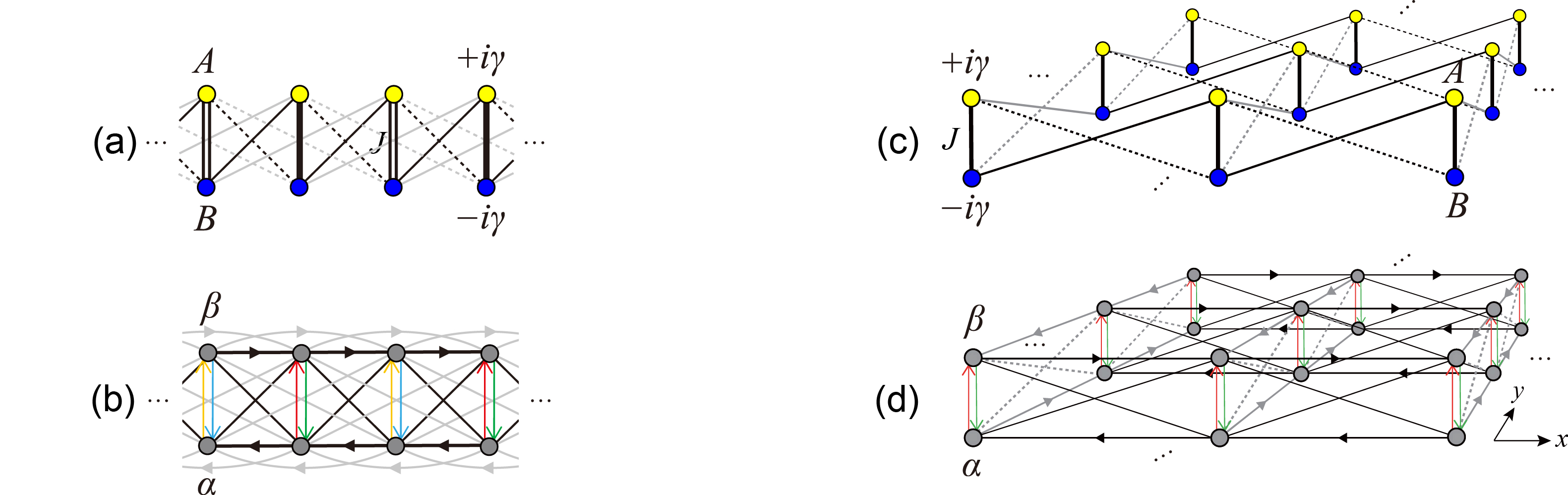
Figure B1: (a) [(c)] Schematic of a bipartite lattice in 1D (2D), the non-Hermitian gain and loss are introduced in the sublattices $A$ and $B$, respectively. (b) [(d)] Schematic of the equivalent lattice of (a) [(c)], the double arrows indicate the asymmetric couplings. For the sake of clarity, the long range couplings in the 2D lattices are not shown in the schematics.

Figure B1(a) depicts a one-dimensional (1D) bipartite lattice. The lines are the couplings between sublattices $A$ and $B$. Each pair of upper and lower sites constitute a dimer. For a dimer with coupling $J$ and balanced gain and loss $\pm i\gamma$, the dimer is $\mathcal{PT}$-symmetric described by $J\sigma_{x}+i\gamma\sigma_{z}$. Applying a unitary transformation

$$U=\left(I_{2}+i\sigma_{x}\right)/\sqrt{2},$$ (B1)

we obtain a non-Hermitian dimer with asymmetric couplings $J\pm\gamma$ in the form of

$$U\left(J\sigma_{x}+i\gamma\sigma_{z}\right)U^{-1}=J\sigma_{x}+i\gamma\sigma_{y}.$$ (B2)

Similarly, the lattice in Figure B1(a) changes into the lattice in Figure B1(b) with asymmetric inter sublattice couplings. The gain and loss change into asymmetric intra dimer couplings (vertical arrows); the inter dimer couplings (slant lines) change to the Hermitian couplings including the inter sublattice reciprocal cross-stitch couplings, and the intra sublattice nonreciprocal couplings with symmetric amplitude (horizontal arrows). The nonreciprocal couplings vanish if inter sublattice couplings in the Hermitian system $H$ are symmetric (the situation that the dashed and solid slant lines are identical). The imaginary gauge field is created at $J\gamma\neq 0$ along the vertical direction, but not along the horizontal direction (translational invariant direction); thus, non-Hermitian AB effect is absent and the bulk-boundary correspondence is valid. The conclusion is applicable in a general situation for systems with nonreciprocal couplings and for higher dimensional bipartite lattices.

In a general case, the topological system may have complex coupling. For a nonreciprocal coupling $Je^{\pm i\phi}$ with Peierls phase $e^{\pm i\phi}$ and coupling amplitude $J$, the $\mathcal{PT}$-symmetric dimer changes to

$$U\left(\begin{array}[]{cc}i\gamma&Je^{-i\phi}\\ Je^{i\phi}&-i\gamma\end{array}\right)U^{-1}$$ (B4)

$$= \left(\begin{array}[]{cc}0&e^{-i\phi}\left(J+\gamma\right)\\ e^{i\phi}\left(J-\gamma\right)&0\end{array}\right),$$ (B7)

where the coupling with symmetric amplitude is changed into coupling with asymmetric amplitude $J+\gamma$ and $J-\gamma$ associated with nonreciprocal Peierls phase $e^{-i\phi}$ and $e^{i\phi}$, respectively. The unitary transformation $U$ applied is

$$U=\frac{1}{\sqrt{2}}\left(\begin{array}[]{cc}1&ie^{-i\phi}\\ ie^{i\phi}&1\end{array}\right).$$ (B8)

In two-dimensional topological systems with chiral symmetry, for instance, a two layer system with inter layer couplings as shown in Figure B1(c), which is a typical bipartite lattice. The non-Hermitian extension is to introduce gain and loss in the upper and lower layers, respectively. Then, the unitary transformation $U$ applied to each corresponding upper and lower sites yields a new two layer lattice as shown in Figure B1(d), the asymmetric couplings only exist between the new two layers (sublattices) after unitary transformation. For higher dimensional systems, the asymmetric couplings still only exist between the two new sublattices after the unitary transformation, which is similar as the one-dimensional and two-dimensional cases. Thus, the nonzero Aharonov-Bohm effect is absent in any translational direction of the topological systems, and the conventional bulk-boundary correspondence holds in the non-Hermitian generalization. The conclusion coincides with that of the mapping theory.

C Mapping of geometric phase and Chern number

In this section, we show that the Berry connection, Berry curvature and Chern number of the non-Hermitian Hamiltonian in the momentum space $\mathcal{H}(\mathbf{k})=H(\mathbf{k})+i\gamma\left(\sigma_{z}\otimes I_{n}\right)$ can be mapped from the Hermitian Hamiltonian $H(\mathbf{k})$ with chiral symmetry by using the mapping matrix. We prove that two topological systems $H(\mathbf{k})$ and $\mathcal{H}(\mathbf{k})$ share an identical Chern number, although their Berry connection and Berry curvature are different. The conclusion is independent of the presence of exceptional points (EPs) in the energy bands.

For the chiral symmetric system $H(\mathbf{k})$, we have

$$\mathcal{S}H(\mathbf{k})\mathcal{S}^{-1}=-H(\mathbf{k}),$$ (C1)

with $\mathcal{S}=\left(\sigma_{z}\otimes I_{n}\right)$. Then, from $H(\mathbf{k})\left|\phi_{\lambda}^{\rho}(\mathbf{k})\right\rangle=\varepsilon_{\lambda}^{\rho}(\mathbf{k})\left|\phi_{\lambda}^{\rho}(\mathbf{k})\right\rangle$, we have $\mathcal{S}H(\mathbf{k})\mathcal{S}^{-1}\mathcal{S}\left|\phi_{\lambda}^{\rho}(\mathbf{k})\right\rangle=\varepsilon_{\lambda}^{\rho}(\mathbf{k})\mathcal{S}\left|\phi_{\lambda}^{\rho}(\mathbf{k})\right\rangle$, which gives $H(\mathbf{k})\left[\mathcal{S}\left|\phi_{\lambda}^{\rho}(\mathbf{k})\right\rangle\right]=-\varepsilon_{\lambda}^{\rho}(\mathbf{k})\left[\mathcal{S}\left|\phi_{\lambda}^{\rho}(\mathbf{k})\right\rangle\right]$. Thus,

$$\left|\phi_{\lambda}^{-\rho}(\mathbf{k})\right\rangle=\mathcal{S}\left|\phi_{\lambda}^{\rho}(\mathbf{k})\right\rangle,$$ (C2)

is the eigenstate for energy $\varepsilon_{\lambda}^{-\rho}(\mathbf{k})=-\varepsilon_{\lambda}^{\rho}(\mathbf{k})$.

We introduce the conventional Berry connection and Berry curvature, which are called the RR Berry connection and Berry curvature Shen . The RR Berry connection for non-Hermitian system $\mathcal{H}(\mathbf{k})$ is

$$\left(\overrightarrow{\mathcal{A}}_{\lambda}^{\rho}\right)_{\mathrm{RR}}=i\left\langle\varphi_{\lambda}^{\rho}(\mathbf{k})\right|\nabla_{\mathbf{k}}\left|\varphi_{\lambda}^{\rho}(\mathbf{k})\right\rangle,$$ (C3)

in which

$$\left|\varphi_{\lambda}^{\rho}(\mathbf{k})\right\rangle=M_{\lambda}^{\rho}(\mathbf{k},\gamma)\left|\phi_{\lambda}^{\rho}(\mathbf{k})\right\rangle,$$ (C4)

and the normalization condition is satisfied, $\left\langle\varphi_{\lambda}^{\rho}(\mathbf{k})\right.\left|\varphi_{\lambda}^{\rho}(\mathbf{k})\right\rangle=1$ under the mapping matrix

$$M_{\lambda}^{\rho}(\mathbf{k},\gamma)=\Pi_{\lambda}^{\rho}(\mathbf{k},\gamma)\left(\begin{array}[]{cc}a_{\lambda}^{\rho}(\mathbf{k},\gamma)I_{n}&0\\ 0&I_{n}\end{array}\right),$$ (C5)

with $\Pi_{\lambda}^{\rho}(\mathbf{k},\gamma)=1$ ($\Pi_{\lambda}^{\rho}(\mathbf{k},\gamma)=\sqrt{2/\{1-\left[a_{\lambda}^{\rho}(\mathbf{k},\gamma)\right]^{2}\}}$) for real (imaginary) $\epsilon_{\lambda}^{\rho}(\mathbf{k})$ to guarantee the normalization condition. Then the RR Berry connection can be written as

$$\left(\overrightarrow{\mathcal{A}}_{\lambda}^{\rho}\right)_{\mathrm{RR}}$$ (C6)

$$= i\left\langle\phi_{\lambda}^{\rho}(\mathbf{k})\right|\left[M_{\lambda}^{\rho}(\mathbf{k},\gamma)\right]^{\dagger}\nabla_{\mathbf{k}}\left[M_{\lambda}^{\rho}(\mathbf{k},\gamma)\left|\phi_{\lambda}^{\rho}(\mathbf{k})\right\rangle\right]$$

$$= i\left\langle\phi_{\lambda}^{\rho}(\mathbf{k})\right|\left[M_{\lambda}^{\rho}(\mathbf{k},\gamma)\right]^{\dagger}M_{\lambda}^{\rho}(\mathbf{k},\gamma)\nabla_{\mathbf{k}}\left|\phi_{\lambda}^{\rho}(\mathbf{k})\right\rangle$$

$$+i\left\langle\phi_{\lambda}^{\rho}(\mathbf{k})\right|\left[M_{\lambda}^{\rho}(\mathbf{k},\gamma)\right]^{\dagger}\left[\nabla_{\mathbf{k}}M_{\lambda}^{\rho}(\mathbf{k},\gamma)\right]\left|\phi_{\lambda}^{\rho}(\mathbf{k})\right\rangle.$$

For real $\epsilon_{\lambda}^{\rho}(\mathbf{k})$, we have $a_{\lambda}^{\rho}(\mathbf{k},\gamma)=e^{i\vartheta}$ with $\vartheta=\arctan\left[\gamma/\epsilon_{\lambda}^{\rho}\left(\mathbf{k}\right)\right]$; then

$$\left[M_{\lambda}^{\rho}(\mathbf{k},\gamma)\right]^{\dagger}M_{\lambda}^{\rho}(\mathbf{k},\gamma)$$ (C11)

$$= \left(\begin{array}[]{cc}e^{-i\vartheta}I_{n}&0\\ 0&I_{n}\end{array}\right)\left(\begin{array}[]{cc}e^{i\vartheta}I_{n}&0\\ 0&I_{n}\end{array}\right)=I_{2n},$$

and

$$\left[M_{\lambda}^{\rho}(\mathbf{k},\gamma)\right]^{\dagger}\nabla_{\mathbf{k}}M_{\lambda}^{\rho}(\mathbf{k},\gamma)$$ (C16)

$$= \left(\begin{array}[]{cc}e^{-i\vartheta}I_{n}&0\\ 0&I_{n}\end{array}\right)\nabla_{\mathbf{k}}\left(\begin{array}[]{cc}e^{i\vartheta}I_{n}&0\\ 0&I_{n}\end{array}\right)$$

$$= \left(\begin{array}[]{cc}I_{n}&0\\ 0&0\end{array}\right)i\nabla_{\mathbf{k}}\vartheta.$$ (C19)

Thus, the RR Berry connection is

$$\left(\overrightarrow{\mathcal{A}}_{\lambda}^{\rho}\right)_{\mathrm{RR}}=\mathbf{A}_{\lambda}^{\rho}-\frac{1}{2}\nabla_{\mathbf{k}}\vartheta,$$ (C20)

with $\mathbf{A}_{\lambda}^{\rho}=i\left\langle\phi_{\lambda}^{\rho}(\mathbf{k})\right|\nabla_{\mathbf{k}}\left|\phi_{\lambda}^{\rho}(\mathbf{k})\right\rangle$ being the Berry connection of the Hermitian system $H\left(\mathbf{k}\right)$.

For imaginary $\epsilon_{\lambda}^{\rho}(\mathbf{k})$, we have $[a_{\lambda}^{\rho}\left(\mathbf{k,}\gamma\right)]^{\ast}=-a_{\lambda}^{\rho}\left(\mathbf{k,}\gamma\right)$,

$$\left[M_{\lambda}^{\rho}(\mathbf{k},\gamma)\right]^{\dagger}M_{\lambda}^{\rho}(\mathbf{k},\gamma)i\nabla_{\mathbf{k}}-I_{2n}i\nabla_{\mathbf{k}}$$ (C23)

$$= \frac{1+\left[a_{\lambda}^{\rho}(\mathbf{k},\gamma)\right]^{2}}{\left[a_{\lambda}^{\rho}(\mathbf{k},\gamma)\right]^{2}-1}\left(\begin{array}[]{cc}I_{n}&0\\ 0&-I_{n}\end{array}\right)i\nabla_{\mathbf{k}}$$

$$= \frac{\epsilon_{\lambda}^{\rho}(\mathbf{k})}{i\gamma}\mathcal{S}i\nabla_{\mathbf{k}},$$ (C24)

and

$$\left[M_{\lambda}^{\rho}(\gamma,\mathbf{k})\right]^{\dagger}\left[\nabla_{\mathbf{k}}M_{\lambda}^{\rho}(\gamma,\mathbf{k})\right] = \left[\Pi_{\lambda}^{\rho}(\mathbf{k},\gamma)\right]^{\ast}\left(\begin{array}[]{cc}\left[a_{\lambda}^{\rho}(\mathbf{k},\gamma)\right]^{\ast}I_{n}&0\\ 0&I_{n}\end{array}\right)\nabla_{\mathbf{k}}\left(\begin{array}[]{cc}a_{\lambda}^{\rho}(\mathbf{k},\gamma)\Pi_{\lambda}^{\rho}(\mathbf{k},\gamma)I_{n}&0\\ 0&\Pi_{\lambda}^{\rho}(\mathbf{k},\gamma)I_{n}\end{array}\right)$$ (C29)

$$= -\frac{1}{2}a_{\lambda}^{\rho}(\mathbf{k},\gamma)\left[\Pi_{\lambda}^{\rho}(\mathbf{k},\gamma)\right]^{4}\left[\nabla_{\mathbf{k}}a_{\lambda}^{\rho}(\mathbf{k},\gamma)\right]\mathcal{S}.$$ (C30)

Then, the RR Berry connection

$$\left(\overrightarrow{\mathcal{A}}_{\lambda}^{\rho}\right)_{\mathrm{RR}} = i\left\langle\phi_{\lambda}^{\rho}(\mathbf{k})\right|\nabla_{\mathbf{k}}\left|\phi_{\lambda}^{\rho}(\mathbf{k})\right\rangle+\frac{\epsilon_{\lambda}^{\rho}(\mathbf{k})}{i\gamma}\left\langle\phi_{\lambda}^{-\rho}(\mathbf{k})\right|\nabla_{\mathbf{k}}\left|\phi_{\lambda}^{\rho}(\mathbf{k})\right\rangle-\frac{1}{2}ia_{\lambda}^{\rho}(\mathbf{k},\gamma)\left[\Pi_{\lambda}^{\rho}(\mathbf{k},\gamma)\right]^{4}\left[\nabla_{\mathbf{k}}a_{\lambda}^{\rho}(\mathbf{\ k},\gamma)\right]\left\langle\phi_{\lambda}^{\rho}(\mathbf{k})\right.\left|\phi_{\lambda}^{-\rho}(\mathbf{k})\right\rangle$$ (C31)

$$= \mathbf{A}_{\lambda}^{\rho}+\frac{\epsilon_{\lambda}^{\rho}(\mathbf{k})}{i\gamma}\left\langle\phi_{\lambda}^{-\rho}(\mathbf{k})\right|\nabla_{\mathbf{k}}\left|\phi_{\lambda}^{\rho}(\mathbf{k})\right\rangle.$$

The definition of RR Berry connection is independent of the biorthonormal basis. Although the eigenstates $\left|\varphi_{\lambda}^{\rho}(\mathbf{k})\right\rangle^{\mathrm{EP}}$ and $\left|\varphi_{\lambda}^{-\rho}(\mathbf{k})\right\rangle^{\mathrm{EP}}$ coalesce at EPs and the biorthonormal basis is absent, the RR Berry connection can still be defined. At EPs, the energy is $\epsilon_{\lambda}^{\rho}(\mathbf{k})^{\mathrm{EP}}=0$, and the mapping matrix has a simple form

$$\left[M_{\lambda}^{\rho}(\mathbf{k},\gamma)\right]^{\mathrm{EP}}=\left(\begin{array}[]{cc}i\rho I_{n}&0\\ 0&I_{n}\end{array}\right).$$ (C32)

Direct derivation shows that the RR Berry connection at EPs is $\left(\overrightarrow{\mathcal{A}}_{\lambda}^{\rho}\right)_{\mathrm{RR}}^{\mathrm{EP}}=i\left\langle\phi_{\lambda}^{\rho}(\mathbf{k})\right|\nabla_{\mathbf{k}}\left|\phi_{\lambda}^{\rho}(\mathbf{\ k})\right\rangle=\mathbf{A}_{\lambda}^{\rho}$.

In conclusion, we have

$$\left(\overrightarrow{\mathcal{A}}_{\lambda}^{\rho}\right)_{\mathrm{RR}}=\left\{\begin{array}[]{ll}\mathbf{A}_{\lambda}^{\rho}-\frac{1}{2}\nabla_{\mathbf{k}}\vartheta,&\text{real }\epsilon_{\lambda}^{\rho}(\mathbf{k})\\ \mathbf{A}_{\lambda}^{\rho}+\left[\mathbf{N}_{\lambda}^{\rho}(\mathbf{k})\right]_{\mathrm{RR}},&\text{imaginary }\epsilon_{\lambda}^{\rho}(\mathbf{k})\\ \mathbf{A}_{\lambda}^{\rho},&\text{at }\mathrm{EPs}\end{array}\right.,$$ (C33)

where $\left[\mathbf{N}_{\lambda}^{\rho}(\mathbf{k})\right]_{\mathrm{RR}}=\epsilon_{\lambda}^{\rho}(\mathbf{k})\left\langle\phi_{\lambda}^{-\rho}(\mathbf{k})\right|\nabla_{\mathbf{k}}\left|\phi_{\lambda}^{\rho}(\mathbf{k})\right\rangle/(i\gamma)$. The RR Berry connection $\left(\overrightarrow{\mathcal{A}}_{\lambda}^{\rho}\right)_{\mathrm{RR}}$ is gauge dependent. If we take the gauge transformation $\left|\varphi_{\lambda}^{\rho}(\mathbf{k})\right\rangle\rightarrow e^{i\chi\left(\mathbf{k}\right)}\left|\varphi_{\lambda}^{\rho}(\mathbf{k})\right\rangle$ with real $\chi\left(\mathbf{k}\right)$, then we have an additional term $i\nabla_{\mathbf{k}}\chi\left(\mathbf{k}\right)$ in $\left(\overrightarrow{\mathcal{A}}_{\lambda}^{\rho}\right)_{\mathrm{RR}}$. However, $\left(\overrightarrow{\mathcal{B}}_{\lambda}^{\rho}\right)_{\mathrm{RR}}=\nabla_{\mathbf{k}}\times\left(\overrightarrow{\mathcal{A}}_{\lambda}^{\rho}\right)_{\mathrm{RR}}$ is gauge independent.

For real $\epsilon_{\lambda}^{\rho}(\mathbf{k})$, we have $\left(\overrightarrow{\mathcal{B}}_{\lambda}^{\rho}\right)_{\mathrm{RR}}=\nabla_{\mathbf{k}}\times\left(\overrightarrow{\mathcal{A}}_{\lambda}^{\rho}\right)_{\mathrm{RR}}=\nabla_{\mathbf{k}}\times\left(\mathbf{A}_{\lambda}^{\rho}-\frac{1}{2}\nabla_{\mathbf{k}}\vartheta\right)=\nabla_{\mathbf{k}}\times\mathbf{A}_{\lambda}^{\rho}=B_{\lambda}^{\rho}$. For imaginary $\epsilon_{\lambda}^{\rho}(\mathbf{k})$, the additional term $\nabla_{\mathbf{k}}\times\left[\mathbf{N}_{\lambda}^{\rho}(\mathbf{k})\right]_{\mathrm{RR}}$ yields zero integration over the Brillouin zone. We prove this as follows. Notice that the eigenstates $\left|\phi_{\lambda}^{\rho}(\mathbf{k})\right\rangle$ and $\left|\phi_{\lambda}^{-\rho}(\mathbf{k})\right\rangle$ can choose an identical gauge in the same region of the Brillouin zone; it is because that the two eigenstates are related through the chiral operator $\mathcal{S}$, and they are orthogonal $\left\langle\phi_{\lambda}^{-\rho}(\mathbf{k})\right.\left|\phi_{\lambda}^{\rho}(\mathbf{k})\right\rangle=0$. If we take a gauge transformation

$$\left|\phi_{\lambda}^{\rho}(\mathbf{k})^{\mathrm{I}}\right\rangle=e^{i\chi\left(\mathbf{k}\right)}\left|\phi_{\lambda}^{\rho}(\mathbf{k})^{\mathrm{II}}\right\rangle,$$ (C34)

then, we have

$$\left|\phi_{\lambda}^{-\rho}(\mathbf{k})^{\mathrm{I}}\right\rangle = \mathcal{S}\left|\phi_{\lambda}^{\rho}(\mathbf{k})^{\mathrm{I}}\right\rangle=\mathcal{S}e^{i\chi\left(\mathbf{k}\right)}\left|\phi_{\lambda}^{\rho}(\mathbf{k})^{\mathrm{II}}\right\rangle$$

$$= e^{i\chi\left(\mathbf{k}\right)}\mathcal{S}\left|\phi_{\lambda}^{\rho}(\mathbf{k})^{\mathrm{II}}\right\rangle=e^{i\chi\left(\mathbf{k}\right)}\left|\phi_{\lambda}^{-\rho}(\mathbf{k})^{\mathrm{II}}\right\rangle.$$

Unlike the Berry connection, term $\left[\mathbf{N}_{\lambda}^{\rho}(\mathbf{k})\right]_{\mathrm{RR}}$ is gauge independent

$$\left[N_{\lambda}^{\rho}(\mathbf{k})^{\mathrm{I}}\right]_{\mathrm{RR}}$$ (C36)

$$= \epsilon_{\lambda}^{\rho}(\mathbf{k})\left\langle\phi_{\lambda}^{-\rho}(\mathbf{k})^{\mathrm{I}}\right|i\nabla_{\mathbf{k}}\left|\phi_{\lambda}^{\rho}(\mathbf{k})^{\mathrm{I}}\right\rangle/\left(i\gamma\right)$$

$$= \epsilon_{\lambda}^{\rho}(\mathbf{k})e^{-i\chi\left(\mathbf{k}\right)}\left\langle\phi_{\lambda}^{-\rho}(\mathbf{k})^{\mathrm{II}}\right|i\nabla_{\mathbf{k}}\left[e^{i\chi\left(\mathbf{k}\right)}\left|\phi_{\lambda}^{\rho}(\mathbf{k})^{\mathrm{II}}\right\rangle\right]/\left(i\gamma\right)$$

$$= \epsilon_{\lambda}^{\rho}(\mathbf{k})e^{-i\chi\left(\mathbf{k}\right)}\left[i\nabla_{\mathbf{k}}e^{i\chi\left(\mathbf{k}\right)}\right]\left\langle\phi_{\lambda}^{-\rho}(\mathbf{k})^{\mathrm{II}}\right.\left|\phi_{\lambda}^{\rho}(\mathbf{k})^{\mathrm{II}}\right\rangle/\left(i\gamma\right)$$

$$+\epsilon_{\lambda}^{\rho}(\mathbf{\ k})\left\langle\phi_{\lambda}^{-\rho}(\mathbf{k})^{\mathrm{II}}\right|i\nabla_{\mathbf{k}}\left|\phi_{\lambda}^{\rho}(\mathbf{k})^{\mathrm{II}}\right\rangle/\left(i\gamma\right)$$

$$= \left[N_{\lambda}^{\rho}(\mathbf{k})^{\mathrm{II}}\right]_{\mathrm{RR}}.$$

One can use different gauges to define the eigenstate if the eigenstate under one gauge is not well-defined in certain regions of the Brillouin zone. We consider a case that the eigenstate of the concerned energy band is well-defined under gauge $\mathrm{I}$ in the region $D^{\mathrm{I}}$ and under gauge $\mathrm{II}$ in the rest region $D^{\mathrm{II}}$ (the cases with more than two gauges required can be similarly generalized). Applying Stokes theorem, we have

$$\oint\nolimits_{\mathrm{BZ}}\nabla_{\mathbf{k}}\times\left[\mathbf{N}_{\lambda}^{\rho}(\mathbf{k})\right]_{\mathrm{RR}}d^{2}\mathbf{k}$$ (C37)

$$= \oint\nolimits_{\partial D^{\mathrm{I}}}\left[\mathbf{N}_{\lambda}^{\rho}(\mathbf{k})\right]_{\mathrm{RR}}^{\mathrm{I}}d\mathbf{k+}\oint\nolimits_{\partial D^{\mathrm{II}}}\left[\mathbf{N}_{\lambda}^{\rho}(\mathbf{k})\right]_{\mathrm{RR}}^{\mathrm{II}}d\mathbf{k}$$

$$= \oint\nolimits_{\partial D^{\mathrm{I}}}\left\{\left[\mathbf{N}_{\lambda}^{\rho}(\mathbf{k})\right]_{\mathrm{RR}}^{\mathrm{I}}-\left[\mathbf{N}_{\lambda}^{\rho}(\mathbf{k})\right]_{\mathrm{RR}}^{\mathrm{II}}\right\}d\mathbf{k}=0.$$

The chiral symmetry of the Hermitian system $H(\mathbf{k})$ plays a crucial role to obtain the above conclusions, the chiral symmetry makes term $\left[\mathbf{N}_{\lambda}^{\rho}(\mathbf{k})\right]_{\mathrm{RR}}$ gauge independent, thus, $\left[\mathbf{N}_{\lambda}^{\rho}(\mathbf{k})\right]_{\mathrm{RR}}$ does not contribute to the Chern number. Based on the above analysis, the RR Chern number of the non-Hermitian system $\mathcal{\ H}(\mathbf{k})$ is exactly identical to the Chern number of the Hermitian system $H(\mathbf{k})$, even though there exists EPs and the energy bands are inseparable (the energy bands of the corresponding Hermitian system are separable, and the Chern number is well defined)

$$\left(c_{\lambda}^{\rho}\right)_{\mathrm{RR}} = \frac{1}{2\pi}\oint\nolimits_{\mathrm{BZ}}\left(\overrightarrow{\mathcal{B}}_{\lambda}^{\rho}\right)_{\mathrm{RR}}d^{2}\mathbf{k}$$ (C38)

$$= \frac{1}{2\pi}\oint\nolimits_{\mathrm{BZ}}\mathbf{B}_{\lambda}^{\rho}d^{2}\mathbf{k}.$$

Now, we discuss the LR Berry connection and Berry curvature based on the biorthonormal basis KawabataPRB98 . $\left|\varphi_{\lambda}^{\rho}(\mathbf{k})\right\rangle$ and $\left|\eta_{\lambda}^{\rho}(\mathbf{k})\right\rangle$ are the eigenstates of $\mathcal{H}(\mathbf{k})$ and $\mathcal{H}^{\dagger}(\mathbf{k})$ with eigenvalues $\epsilon_{\lambda}^{\rho}(\mathbf{k})$ and $\left[\epsilon_{\lambda}^{\rho}(\mathbf{k})\right]^{\ast}$, respectively. The Schrödinger equations are

$$\mathcal{H}\left(\mathbf{k}\right)\left|\varphi_{\lambda}^{\rho}(\mathbf{k})\right\rangle = \epsilon_{\lambda}^{\rho}(\mathbf{k})\left|\varphi_{\lambda}^{\rho}(\mathbf{k})\right\rangle,$$ (C39)

$$\mathcal{H}^{\dagger}\left(\mathbf{k}\right)\left|\eta_{\lambda}^{\rho}(\mathbf{k})\right\rangle = \left[\epsilon_{\lambda}^{\rho}(\mathbf{k})\right]^{\ast}\left|\eta_{\lambda}^{\rho}(\mathbf{k})\right\rangle.$$ (C40)

The eigenstates $\left\{\left|\varphi_{\lambda}^{\rho}(\mathbf{k})\right\rangle,\left|\eta_{\lambda}^{\rho}(\mathbf{k})\right\rangle\right\}$ can be mapped from the eigenstates of the original Hermitian system $H\left(\mathbf{k}\right)$,

$$\left|\varphi_{\lambda}^{\rho}(\mathbf{k})\right\rangle = M_{\lambda}^{\rho}(\mathbf{k},\gamma)\left|\phi_{\lambda}^{\rho}(\mathbf{k})\right\rangle,$$ (C41)

$$\left|\eta_{\lambda}^{\rho}(\mathbf{k})\right\rangle = \left[M_{\lambda}^{\rho}(\mathbf{k},\gamma)\right]^{\dagger}\left|\phi_{\lambda}^{\rho}(\mathbf{k})\right\rangle.$$ (C42)

In the absence of EP, the mapping matrix can be written as

$$M_{\lambda}^{\rho}(\mathbf{k},\gamma)=\Lambda_{\lambda}^{\rho}(\mathbf{\ k},\gamma)\left(\begin{array}[]{cc}a_{\lambda}^{\rho}(\mathbf{k},\gamma)I_{n}&0\\ 0&I_{n}\end{array}\right),$$ (C43)

with $\Lambda_{\lambda}^{\rho}(\mathbf{k},\gamma)=\sqrt{2/\{1+\left[a_{\lambda}^{\rho}(\mathbf{k},\gamma)\right]^{2}\}}$ to guarantee the biorthonormal normalization.

Based on the orthonormal relation $\langle\phi_{\lambda}^{\rho}(\mathbf{k})|\phi_{\lambda^{\prime}}^{\rho^{\prime}}(\mathbf{k}^{\prime})\rangle=\delta_{\mathbf{kk}^{\prime}}\delta_{\lambda\lambda^{\prime}}\delta_{\rho\rho^{\prime}}$ for the eigenstates of the original Hermitian system, we have the biorthonormal relation

$$\langle\eta_{\lambda}^{\rho}(\mathbf{k})|\varphi_{\lambda^{\prime}}^{\rho^{\prime}}(\mathbf{k}^{\prime})\rangle=\delta_{\mathbf{kk}^{\prime}}\delta_{\lambda\lambda^{\prime}}\delta_{\rho\rho^{\prime}},$$ (C44)

for the left and right eigenstates of the non-Hermitian system.

The Berry connection based on the left and right eigenstates is defined as

$$\left(\overrightarrow{\mathcal{A}}_{\lambda}^{\rho}\right)_{\mathrm{LR}} = i\left\langle\eta_{\lambda}^{\rho}(\mathbf{k})\right|\nabla_{\mathbf{k}}\left|\varphi_{\lambda}^{\rho}(\mathbf{k})\right\rangle$$

$$= i\left\langle\phi_{\lambda}^{\rho}(\mathbf{k})\right|M_{\lambda}^{\rho}(\mathbf{k},\gamma)\nabla_{\mathbf{k}}\left[M_{\lambda}^{\rho}(\mathbf{k},\gamma)\left|\phi_{\lambda}^{\rho}(\mathbf{k})\right\rangle\right]$$

$$= i\left\langle\phi_{\lambda}^{\rho}(\mathbf{k})\right|\left[M_{\lambda}^{\rho}(\mathbf{k},\gamma)\right]^{2}\nabla_{\mathbf{k}}\left|\phi_{\lambda}^{\rho}(\mathbf{k})\right\rangle$$

$$+i\left\langle\phi_{\lambda}^{\rho}(\mathbf{k})\right|M_{\lambda}^{\rho}(\mathbf{\ k},\gamma)\left[\nabla_{\mathbf{k}}M_{\lambda}^{\rho}(\mathbf{k},\gamma)\right]\left|\phi_{\lambda}^{\rho}(\mathbf{k})\right\rangle,$$

where

$$M_{\lambda}^{\rho}(\mathbf{k},\gamma)\left[\nabla_{\mathbf{k}}M_{\lambda}^{\rho}(\mathbf{k},\gamma)\right] = \Lambda_{\lambda}^{\rho}(\mathbf{k},\gamma)\left(\begin{array}[]{cc}a_{\lambda}^{\rho}(\mathbf{k},\gamma)I_{n}&0\\ 0&I_{n}\end{array}\right)\nabla_{\mathbf{k}}\left(\begin{array}[]{cc}a_{\lambda}^{\rho}(\mathbf{k},\gamma)\Lambda_{\lambda}^{\rho}(\mathbf{k},\gamma)I_{n}&0\\ 0&\Lambda_{\lambda}^{\rho}(\mathbf{k},\gamma)I_{n}\end{array}\right)$$ (C50)

$$= \frac{1}{2}a_{\lambda}^{\rho}(\mathbf{k},\gamma)\left[\Lambda_{\lambda}^{\rho}(\mathbf{k},\gamma)\right]^{4}\left[\nabla_{\mathbf{k}}a_{\lambda}^{\rho}(\mathbf{k},\gamma)\right]\mathcal{S},$$ (C51)

and

$$\left[M_{\lambda}^{\rho}(\mathbf{k},\gamma)\right]^{2}i\nabla_{\mathbf{\ k}}-I_{2n}i\nabla_{\mathbf{k}}$$ (C54)

$$= \frac{\left[a_{\lambda}^{\rho}(\mathbf{k},\gamma)\right]^{2}-1}{1+\left[a_{\lambda}^{\rho}(\mathbf{k},\gamma)\right]^{2}}\left(\begin{array}[]{cc}I_{n}&0\\ 0&-I_{n}\end{array}\right)i\nabla_{\mathbf{k}}$$

$$= \frac{i\gamma}{\epsilon_{\lambda}^{\rho}(\mathbf{k})}\mathcal{S}i\nabla_{\mathbf{k}}.$$ (C55)

Thus, the Berry connection is reduced to

$$\left(\overrightarrow{\mathcal{A}}_{\lambda}^{\rho}\right)_{\mathrm{LR}} = i\left\langle\phi_{\lambda}^{\rho}(\mathbf{k})\right|\left[M_{\lambda}^{\rho}(\mathbf{k},\gamma)\right]^{2}\nabla_{\mathbf{k}}\left|\phi_{\lambda}^{\rho}(\mathbf{k})\right\rangle$$ (C56)

$$+ i\left\langle\phi_{\lambda}^{\rho}(\mathbf{k})\right|M_{\lambda}^{\rho}(\mathbf{\ k},\gamma)\left[\nabla_{\mathbf{k}}M_{\lambda}^{\rho}(\mathbf{k},\gamma)\right]\left|\phi_{\lambda}^{\rho}(\mathbf{k})\right\rangle$$

$$= \mathbf{A}_{\lambda}^{\rho}+\frac{i\gamma}{\epsilon_{\lambda}^{\rho}(\mathbf{k})}\left\langle\phi_{\lambda}^{-\rho}(\mathbf{k})\right|i\nabla_{\mathbf{k}}\left|\phi_{\lambda}^{\rho}(\mathbf{k})\right\rangle$$

$$+ \frac{1}{2}ia_{\lambda}^{\rho}\left[\Lambda_{\lambda}^{\rho}(\mathbf{k},\gamma)\right]^{4}\left[\nabla_{\mathbf{k}}a_{\lambda}^{\rho}(\mathbf{k},\gamma)\right]\left\langle\phi_{\lambda}^{-\rho}(\mathbf{k})\right.\left|\phi_{\lambda}^{\rho}(\mathbf{k})\right\rangle$$

$$= \mathbf{A}_{\lambda}^{\rho}+\left[\mathbf{N}_{\lambda}^{\rho}(\mathbf{k})\right]_{\mathrm{LR}},$$

where $\mathbf{A}_{\lambda}^{\rho}=i\left\langle\phi_{\lambda}^{\rho}(\mathbf{k})\right|\nabla_{\mathbf{k}}\left|\phi_{\lambda}^{\rho}(\mathbf{k})\right\rangle$ is the Berry connection for the original Hamiltonian $H(\mathbf{k})$, and

$$\left[\mathbf{N}_{\lambda}^{\rho}(\mathbf{k})\right]_{\mathrm{LR}}=i\gamma\left\langle\phi_{\lambda}^{-\rho}(\mathbf{k})\right|i\nabla_{\mathbf{k}}\left|\phi_{\lambda}^{\rho}(\mathbf{k})\right\rangle/\epsilon_{\lambda}^{\rho}(\mathbf{k}).$$ (C57)

The LR Berry connection $\left(\overrightarrow{\mathcal{A}}_{\lambda}^{\rho}\right)_{\mathrm{LR}}$ is gauge dependent. For instance, if we take the transformation $\left|\varphi_{\lambda}^{\rho}(\mathbf{k})\right\rangle\rightarrow e^{i\chi\left(\mathbf{k}\right)}\left|\varphi_{\lambda}^{\rho}(\mathbf{k})\right\rangle$ and $\left|\eta_{\lambda}^{\rho}(\mathbf{k})\right\rangle\rightarrow e^{i\chi\left(\mathbf{k}\right)}\left|\eta_{\lambda}^{\rho}(\mathbf{k})\right\rangle$, the biorthonormal relation still holds; in contrast, we have an additional term $i\nabla_{\mathbf{k}}\chi\left(\mathbf{k}\right)$ in $\left(\overrightarrow{\mathcal{A}}_{\lambda}^{\rho}\right)_{\mathrm{LR}}$.

The Berry curvature has the form

$$\left(\overrightarrow{\mathcal{B}}_{\lambda}^{\rho}\right)_{\mathrm{LR}} = \nabla_{\mathbf{k}}\times\overrightarrow{\mathcal{A}}_{\lambda}^{\rho}$$ (C58)

$$= \mathbf{B}_{\lambda}^{\rho}+\nabla_{\mathbf{k}}\times\left[\mathbf{N}_{\lambda}^{\rho}(\mathbf{k})\right]_{\mathrm{LR}},$$

where $\mathbf{B}_{\lambda}^{\rho}=\nabla_{\mathbf{k}}\times\mathbf{A}_{\lambda}^{\rho}$. Equation (C58) means that the Berry curvature of $\mathcal{H}(\mathbf{k})$ is complex or real for real or imaginary $\epsilon_{\lambda}^{\rho}(\mathbf{k})$. The additional term $\nabla_{\mathbf{k}}\times\left[\mathbf{N}_{\lambda}^{\rho}(\mathbf{k})\right]_{\mathrm{LR}}$ yields zero integration over the Brillouin zone as we have shown in the RR case, which means that the Chern numbers of $H(\mathbf{k})$ and $\mathcal{H}(\mathbf{k})$ are identical

$$\left(c_{\lambda}^{\rho}\right)_{\mathrm{LR}} = \frac{1}{2\pi}\oint\nolimits_{\mathrm{BZ}}\left(\overrightarrow{\mathcal{B}}_{\lambda}^{\rho}\right)_{\mathrm{LR}}d^{2}\mathbf{k}$$ (C59)

$$= \frac{1}{2\pi}\oint\nolimits_{\mathrm{BZ}}\mathbf{B}_{\lambda}^{\rho}d^{2}\mathbf{k}.$$

Integral in Eq. (C59) is under the assumption that EPs are absent in the Brillouin zone, since the biorthonormal basis does not exist at EPs.

Besides the RR and LR definitions, one can also define the RL and LL Berry connections and Berry curvatures. For the Hermitian and corresponding non-Hermitian topological systems we concerned, the RL and LL Berry connections are

$$\left(\overrightarrow{\mathcal{A}}_{\lambda}^{\rho}\right)_{\mathrm{RL}} = i\left\langle\varphi_{\lambda}^{\rho}(\mathbf{k})\right|\nabla_{\mathbf{k}}\left|\eta_{\lambda}^{\rho}(\mathbf{k})\right\rangle=\mathbf{A}_{\lambda}^{\rho}-\frac{i\gamma}{\epsilon_{\lambda}^{\rho}(\mathbf{k})}\left\langle\phi_{\lambda}^{-\rho}(\mathbf{k})\right|i\nabla_{\mathbf{k}}\left|\phi_{\lambda}^{\rho}(\mathbf{k})\right\rangle,$$ (C60)

$$\left(\overrightarrow{\mathcal{A}}_{\lambda}^{\rho}\right)_{\mathrm{LL}} = i\left\langle\eta_{\lambda}^{\rho}(\mathbf{k})\right|\nabla_{\mathbf{k}}\left|\eta_{\lambda}^{\rho}(\mathbf{k})\right\rangle=\left\{\begin{array}[]{ll}\mathbf{A}_{\lambda}^{\rho}+\frac{1}{2}\nabla_{\mathbf{k}}\vartheta,&\text{real }\epsilon_{\lambda}^{\rho}(\mathbf{k})\\ \mathbf{A}_{\lambda}^{\rho}-\epsilon_{\lambda}^{\rho}(\mathbf{k})\left\langle\phi_{\lambda}^{-\rho}(\mathbf{k})\right|i\nabla_{\mathbf{k}}\left|\phi_{\lambda}^{\rho}(\mathbf{k})\right\rangle/\left(i\gamma\right),&\text{imaginary }\epsilon_{\lambda}^{\rho}(\mathbf{k})\\ \mathbf{A}_{\lambda}^{\rho},&\text{at }\mathrm{EPs}\end{array}\right.,$$ (C64)

and the four definitions of the Chern number are identical for separated bands (i.e., in the absence of EPs) Shen .

D Details of the 1D comb lattice model

D.1 Model and energy bands

The non-Hermitian Hamiltonian of the one-dimensional comb lattice model reads

$$\mathcal{H}=H+i\gamma\sum_{j=1}^{2N}(a_{j}^{\dagger}a_{j}-b_{j}^{\dagger}b_{j}),$$ (D1)

which is generated from the Hermitian Hamiltonian

$$H = \sum_{j=1}^{N}[J\left(1-\delta\right)a_{2j}^{\dagger}b_{2j-1}+J\left(1+\delta\right)a_{2j}^{\dagger}b_{2j+1}]$$ (D2)

$$+\sum_{j=1}^{N}\kappa_{-}a_{2j-1}^{\dagger}b_{2j-1}+\sum_{j=1}^{N}\kappa_{+}a_{2j}^{\dagger}b_{2j}+\mathrm{H.c.},$$

under the periodic boundary condition $b_{2N+1}=b_{1}$, and the system parameters are $\delta=\delta_{0}+R\cos\theta$ and $\kappa_{\pm}=\kappa_{0}\pm(1/2)R\sin\theta$ (set $\kappa\equiv\kappa_{+}-\kappa_{-}=R\sin\theta$). We refer to the Hamiltonian with periodic boundary condition as the bulk Hamiltonian, and the edge Hamiltonian is the Hamiltonian under open boundary condition. Taking the Fourier transformation

$$\left(\begin{array}[]{c}a_{2j}\\ a_{2j-1}\\ b_{2j-1}\\ b_{2j}\end{array}\right)=\frac{1}{\sqrt{N}}\sum_{k}e^{ikj}\left(\begin{array}[]{c}a_{k,+}\\ a_{k,-}\\ b_{k,+}\\ b_{k,-}\end{array}\right),$$ (D3)

we obtain

$$H = \sum_{k}\alpha_{k}^{{\dagger}}H(k)\alpha_{k},$$ (D4)

$$\mathcal{H} = \sum_{k}\alpha_{k}^{{\dagger}}\mathcal{H}(k)\alpha_{k},$$ (D5)

where $\alpha_{k}^{{\dagger}}=\left(a_{k,+}^{\dagger},a_{k,-}^{\dagger},b_{k,+}^{\dagger},b_{k,-}^{\dagger}\right)$, and the $4\times 4$ matrix $\mathcal{H}(k)$ and $H(k)$ has the form

$$\mathcal{H}(k) = H(k)+i\gamma\sigma_{z}\otimes I_{2}$$ (D10)

$$= \left(\begin{array}[]{cccc}i\gamma&0&\mu_{k}&\kappa_{+}\\ 0&i\gamma&\kappa_{-}&0\\ \mu_{-k}&\kappa_{-}&-i\gamma&0\\ \kappa_{+}&0&0&-i\gamma\end{array}\right),$$

with $\mu_{k}=J\left(1-\delta\right)+J\left(1+\delta\right)e^{ik}$, $k_{m}=2\pi m/N$, $(m=1,2,...,N)$. The eigenstates of $H(k)$ has the form

$$|\phi_{\lambda}^{\rho}(k)\rangle=\frac{1}{\Omega_{\lambda}^{\rho}(k)}\left(\begin{array}[]{c}\varepsilon_{\lambda}^{\rho}(k)\kappa_{-}\mu_{k}\\ \varepsilon_{\lambda}^{-\rho}(k)[\varepsilon_{-\lambda}^{\rho}(k)^{2}-\kappa_{-}^{2}]\\ \kappa_{-}[\varepsilon_{\lambda}^{\rho}(k)^{2}-\kappa_{+}^{2}]\\ \kappa_{+}\kappa_{-}\mu_{k}\end{array}\right),$$ (D11)

where $\Omega_{\lambda}^{\rho}(k)=\sqrt{2}\kappa_{-}\varepsilon_{\lambda}^{\rho}(k)^{-1}\{[\varepsilon_{\lambda}^{\rho}(k)^{4}-\left(\kappa_{+}\kappa_{-}\right)^{2}][\varepsilon_{\lambda}^{\rho}(k)^{2}-\left(\kappa_{+}\right)^{2}]\}^{1/2}$ is the normalization factor and $\left(\rho,\lambda=\pm\right)$. The corresponding eigenvalue is

$$\varepsilon_{\lambda}^{\rho}(k)=\rho\{\Upsilon_{k}+\lambda[\Upsilon_{k}^{2}-\left(\kappa_{+}\kappa_{-}\right)^{2}]^{\frac{1}{2}}\}^{\frac{1}{2}},$$ (D12)

with $\Upsilon_{k}=(\left|\mu_{k}\right|^{2}+\kappa_{+}^{2}+\kappa_{-}^{2})/2$.

The energy bands are depicted in Fig. D1 at various $\gamma$ as the supplementary of Figs. 2(a) and 2(b) in the main text.

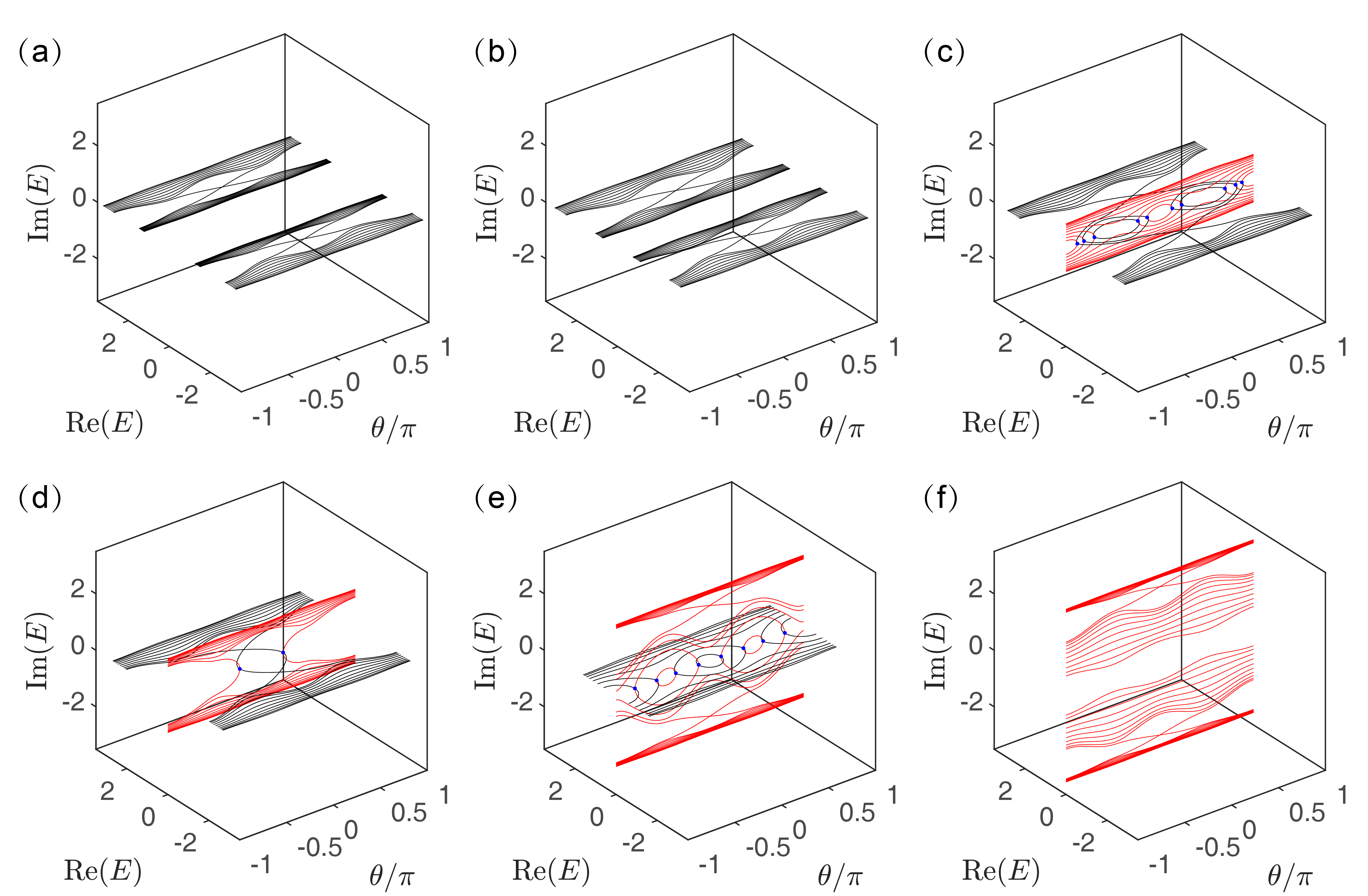
Figure D1: Energy bands of the edge Hamiltonian for $\delta_{0}=0$ at (a) $\gamma=0$, (b) $\gamma=1.0$, (c) $\gamma=1.5$, (d) $\gamma=1.8$, (e) $\gamma=2.8$, (f) $\gamma=3.3$ . The real (imaginary) part is in black (red), the blue dots are EPs. Other parameters are $J=1$, $\kappa_{0}=2$, $R=0.6$, and $N=10$.

D.2 Zak phase

In the condition of $\kappa_{+}=\kappa_{-}=\kappa_{0}$ ($\theta=0$), the eigenstates of $\mathcal{H}(k)$ are

$$\left|\varphi_{\lambda}^{\rho}(k)\right\rangle=M_{\lambda}^{\rho}\left(k,\gamma\right)\left|\phi_{\lambda}^{\rho}(k)\right\rangle,$$ (D13)

where

$$|\phi_{\lambda}^{\rho}(k)\rangle=\frac{1}{\Omega_{\lambda}^{\rho}(k)}\left(\begin{array}[]{c}\varepsilon_{\lambda}^{\rho}(k)\kappa_{0}\mu_{k}\\ \varepsilon_{\lambda}^{-\rho}(k)[\varepsilon_{-\lambda}^{\rho}(k)^{2}-\kappa_{0}^{2}]\\ \kappa_{0}[\varepsilon_{\lambda}^{\rho}(k)^{2}-\kappa_{0}^{2}]\\ \kappa_{0}^{2}\mu_{k}\end{array}\right),$$ (D14)

are the eigenstates of $H(k)$, and

$$M_{\lambda}^{\rho}\left(k,\gamma\right) = \sqrt{\frac{2}{1+e^{2i\vartheta}}}\left(\begin{array}[]{cccc}e^{i\vartheta}&0&0&0\\ 0&e^{i\vartheta}&0&0\\ 0&0&1&0\\ 0&0&0&1\end{array}\right),$$ (D19)

$$\vartheta = \arctan\left[\gamma/\epsilon_{\lambda}^{\rho}\left(k\right)\right].$$ (D20)

Similarly, the eigenstates of $\mathcal{H}^{\dagger}(k)$ are

$$\left|\eta_{\lambda}^{\rho}(k)\right\rangle=\left[M_{\lambda}^{\rho}\left(k,\gamma\right)\right]^{\dagger}\left|\phi_{\lambda}^{\rho}\right\rangle.$$ (D21)

By definition, the Berry connection of the non-Hermitian system reads

$$\mathcal{A}_{\lambda}^{\rho}=i\left\langle\eta_{\lambda}^{\rho}(k)\right|\partial_{k}\left|\varphi_{\lambda}^{\rho}(k)\right\rangle,$$ (D22)

in which, the right and left eigenstates can be written as

$$\left|\varphi_{\lambda}^{\rho}(k)\right\rangle = S\left(\delta\right)M_{\lambda}^{\rho}\left(k,\gamma\right)\left|\Phi_{\lambda}^{\rho}(k)\right\rangle,$$ (D23)

$$\left|\eta_{\lambda}^{\rho}(k)\right\rangle = S\left(\delta\right)\left[M_{\lambda}^{\rho}\left(k,\gamma\right)\right]^{\dagger}\left|\Phi_{\lambda}^{\rho}\right\rangle,$$ (D24)

with

$$S\left(\delta\right)=\left(\begin{array}[]{cccc}\mu_{k}&0&0&0\\ 0&1&0&0\\ 0&0&1&0\\ 0&0&0&\mu_{k}\end{array}\right),$$ (D25)

and

$$\left|\Phi_{\lambda}^{\rho}(k)\right\rangle=\frac{1}{\Omega_{\lambda}^{\rho}(k)}\left(\begin{array}[]{c}\varepsilon_{\lambda}^{\rho}(k)\kappa_{0}\\ \varepsilon_{\lambda}^{-\rho}(k)\left[\varepsilon_{-\lambda}^{\rho}(k)^{2}-\kappa_{0}^{2}\right]\\ \kappa_{0}\left[\varepsilon_{\lambda}^{\rho}(k)^{2}-\kappa_{0}^{2}\right]\\ \kappa_{0}^{2}\end{array}\right).$$ (D26)

Then the Zak phase $\mathcal{Z}_{\lambda}^{\rho}\left(\delta\right)=\int_{-\pi}^{\pi}\mathcal{A}_{\lambda}^{\rho}dk$,

$$\mathcal{Z}_{\lambda}^{\rho}\left(\delta\right) = i\int_{-\pi}^{\pi}\left\langle\Phi_{\lambda}^{\rho}(k)\right|M_{\lambda}^{\rho}\left(k,\gamma\right)S^{\dagger}\left(\delta\right)\partial_{k}\left[S\left(\delta\right)M_{\lambda}^{\rho}\left(k,\gamma\right)\left|\Phi_{\lambda}^{\rho}(k)\right\rangle\right]dk$$ (D27)

$$= i\int_{-\pi}^{\pi}\left\langle\Phi_{\lambda}^{\rho}(k)\right|M_{\lambda}^{\rho}\left(k,\gamma\right)S^{\dagger}\left(\delta\right)\left[\partial_{k}S\left(\delta\right)\right]M_{\lambda}^{\rho}\left(k,\gamma\right)\left|\Phi_{\lambda}^{\rho}(k)\right\rangle dk$$

$$+i\int_{-\pi}^{\pi}\left\langle\Phi_{\lambda}^{\rho}(k)\right|M_{\lambda}^{\rho}\left(k,\gamma\right)S^{\dagger}\left(\delta\right)S\left(\delta\right)\partial_{k}\left[M_{\lambda}^{\rho}\left(k,\gamma\right)\left|\Phi_{\lambda}^{\rho}(k)\right\rangle\right]dk.$$

We note that $\left|\mu_{k}\left(\delta\right)\right|^{2}=\left|\mu_{k}\left(-\delta\right)\right|^{2}=4J^{2}\left[\cos^{2}\left(k/2\right)+\delta^{2}\sin^{2}\left(k/2\right)\right]$ and $\varepsilon_{\lambda}^{\rho}\left(k,\delta\right)=\varepsilon_{\lambda}^{\rho}\left(k,-\delta\right)$, then

$$S^{\dagger}\left(\delta\right)S\left(\delta\right) = \left(\begin{array}[]{cccc}\left|\mu_{k}\left(\delta\right)\right|^{2}&0&0&0\\ 0&1&0&0\\ 0&0&1&0\\ 0&0&0&\left|\mu_{k}\left(\delta\right)\right|^{2}\end{array}\right)=S^{\dagger}\left(\left|\delta\right|\right)S\left(\left|\delta\right|\right),$$ (D32)

$$\varepsilon_{\lambda}^{\rho}\left(k,\delta\right) = \varepsilon_{\lambda}^{\rho}\left(k,\left|\delta\right|\right),$$ (D33)

which means $\left\langle\Phi_{\lambda}^{\rho}\left(k\right)\right|M_{\lambda}^{\rho}\left(k,\gamma\right)S^{\dagger}\left(\delta\right)S\left(\delta\right)\partial_{k}\left[M_{\lambda}^{\rho}\left(k,\gamma\right)\left|\Phi_{\lambda}^{\rho}\left(k\right)\right\rangle\right]$ is the function of $\left|\delta\right|$, so we have

$$\mathcal{Z}_{\lambda}^{\rho}\left(\delta\right)-\mathcal{Z}_{\lambda}^{\rho}\left(-\delta\right)=i\int_{-\pi}^{\pi}\left\langle\Phi_{\lambda}^{\rho}\right|M_{\lambda}^{\rho}\left(\gamma\right)\left[S^{\dagger}\left(\delta\right)\partial_{k}S\left(\delta\right)-S^{\dagger}\left(-\delta\right)\partial_{k}S\left(-\delta\right)\right]M_{\lambda}^{\rho}\left(\gamma\right)\left|\Phi_{\lambda}^{\rho}\right\rangle dk.$$ (D34)

Direct derivation shows that

$$\mathcal{Z}_{\lambda}^{\rho}\left(\delta\right)-\mathcal{Z}_{\lambda}^{\rho}\left(-\delta\right)=-8\delta J^{2}\kappa_{0}^{2}\int_{-\pi}^{\pi}\frac{\varepsilon_{\lambda}^{\rho}(k)^{2}e^{2i\vartheta}+\kappa_{0}^{2}}{\Omega_{\lambda}^{\rho}(k)^{2}\left(1+e^{2i\vartheta}\right)}dk.$$ (D35)

Furthermore, using $e^{i\vartheta}=\left[\epsilon_{\lambda}^{\rho}(k)+i\gamma\right]/\varepsilon_{\lambda}^{\rho}(k),\epsilon_{\lambda}^{\rho}(k)=\rho\sqrt{\varepsilon_{\lambda}^{\rho}(k)^{2}-\gamma^{2}},1+e^{2i\vartheta}=2e^{i\vartheta}\cos\vartheta,$and $\tan\vartheta=\gamma/\epsilon_{\lambda}^{\rho}(k)$, $\mathcal{Z}_{\lambda}^{\rho}\left(\delta\right)-\mathcal{Z}_{\lambda}^{\rho}\left(-\delta\right)$ is reduced to

$$\mathcal{Z}_{\lambda}^{\rho}\left(\delta\right)-\mathcal{Z}_{\lambda}^{\rho}\left(-\delta\right)=-\mathrm{sgn}\left(\delta\right)\pi-2i\gamma\rho\delta J^{2}\int_{-\pi}^{\pi}\frac{[\varepsilon_{\lambda}^{\rho}(k)]^{2}}{\sqrt{\varepsilon_{\lambda}^{\rho}(k)^{2}-\gamma^{2}}\left[\varepsilon_{\lambda}^{\rho}(k)^{4}-\kappa_{0}^{4}\right]}dk,$$ (D36)

where the later term is imaginary and non-vanished for non-Hermitian Hamiltonian; however, for $[\varepsilon_{\lambda}^{\rho}(k)]^{2}=[\varepsilon_{\lambda}^{-\rho}(k)]^{2}$, the summation $\frac{1}{\pi}\sum_{\rho\lambda}\left[\mathcal{Z}_{\lambda}^{\rho}\left(\delta\right)-\mathcal{Z}_{\lambda}^{\rho}\left(-\delta\right)\right]$ is an integer HJiang . Zak phase is a physical interpretation of the Chern number, since the adiabatic transport of particle is regarded as a manifestation of Zak phase.

D.3 Edge states

The non-Hermitian Hamiltonian under open boundary condition is the edge Hamiltonian

$$\mathcal{H}_{\mathrm{edge}}=\mathcal{H}-J\left(1+\delta\right)\left(a_{2N}^{\dagger}b_{1}+b_{1}^{\dagger}a_{2N}\right).$$ (D37)

The original Hermitian edge Hamiltonian possesses four edge states WRPRB , from which we can obtain the corresponding edge states of the non-Hermitian system by using the mapping method. The four edge states of $\mathcal{H}_{\mathrm{edge}}$ can be expressed as

$$\left\{\begin{array}[]{c}\left|\varphi_{\mathrm{R}}^{\pm}\right\rangle=\frac{1}{\sqrt{\Omega}}\sum\limits_{j=1}^{N}\varsigma^{N-j}(e^{\pm i\vartheta_{\mathrm{R}}}a_{2j}^{\dagger}\pm b_{2j}^{\dagger})\left|\text{{vac}}\right\rangle\\ \left|\varphi_{\mathrm{L}}^{\pm}\right\rangle=\frac{1}{\sqrt{\Omega}}\sum\limits_{j=1}^{N}\varsigma^{j-1}(e^{\pm i\vartheta_{\mathrm{L}}}a_{2j-1}^{\dagger}\pm b_{2j-1}^{\dagger})\left|\text{{vac}}\right\rangle\end{array}\right.,$$ (D38)

with eigenenergies

$$\left\{\begin{array}[]{c}\epsilon_{\mathrm{R}}^{\pm}=\pm\sqrt{\left(\kappa_{+}\right)^{2}-\gamma^{2}}\\ \epsilon_{\mathrm{L}}^{\pm}=\pm\sqrt{\left(\kappa_{-}\right)^{2}-\gamma^{2}}\end{array}\right..$$ (D39)

Here $\varsigma=(\delta-1)/(\delta+1)$, $\Omega=2(1-\varsigma^{2N})/(1-\varsigma^{2})$, $e^{\pm i\vartheta_{\mathrm{R}}}=(\epsilon_{\mathrm{R}}^{+}\pm i\gamma)/\kappa_{+}$ and $e^{\pm i\vartheta_{\mathrm{L}}}=(\epsilon_{\mathrm{L}}^{+}\pm i\gamma)/\kappa_{-}$.

E Topological charge pumping

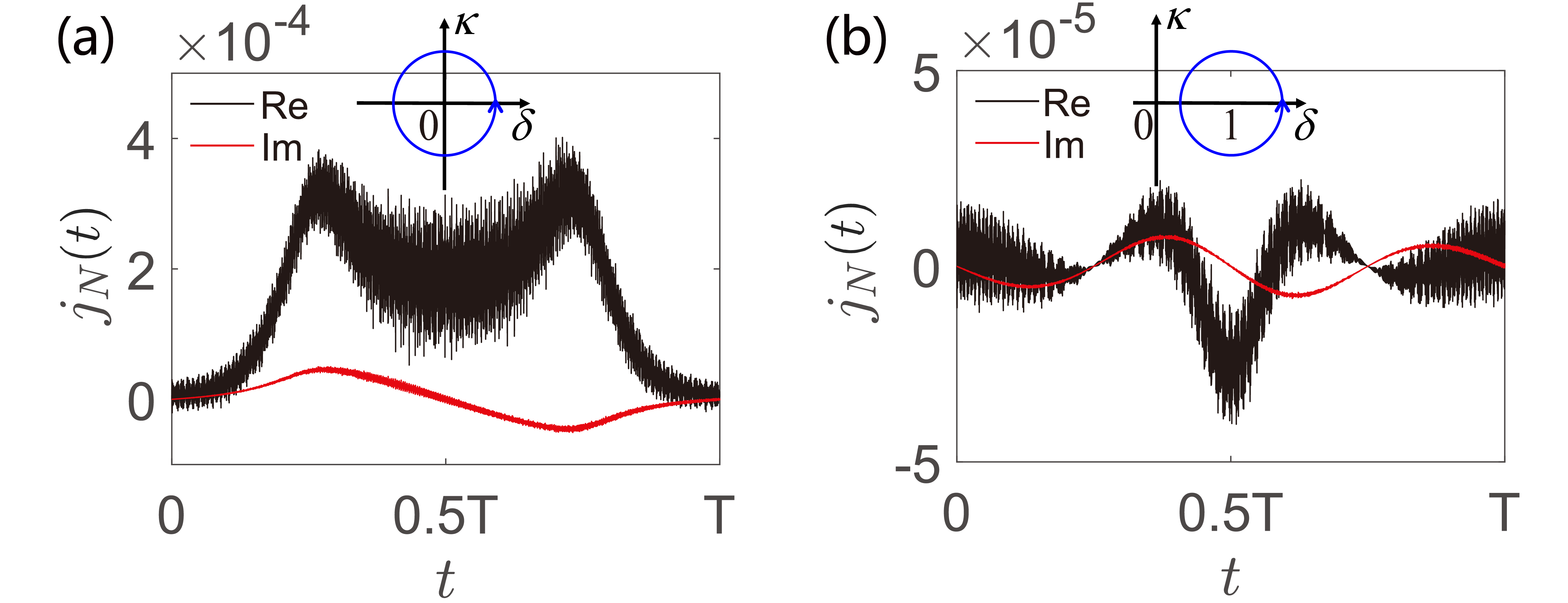
Figure E1: Particle current $j_{N}(t)$ for the numerical simulations in Figs. 1(b) and 1(c) of the main text for $\mathcal{H}\left(t\right)$. Numerical simulations are performed for (a) topological nontrivial phase $R>\left|\delta_{0}\right|$ at $\delta_{0}=0$ and (b) topological trivial phase $R<\left|\delta_{0}\right|$ at $\delta_{0}=1$. The speed of time evolution is $\omega=0.001$ and the period is $T=2\pi\omega^{-1}$. Other parameters are $\gamma=0.5$, $J=1$, $R=0.6$, and $N=10$. Two quasi-adiabatic processes are illustrated in the insets.

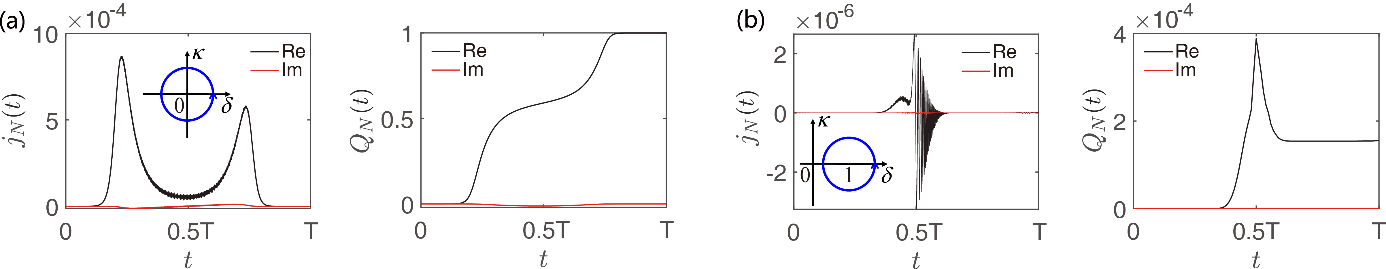
Figure E2: Particle current $j_{N}(t)$ and topological charge pumping $Q_{N}(t)$ for the edge states of $\mathcal{H}_{\mathrm{edge}}(t)$. Numerical simulations are performed for (a) topological nontrivial phase $R>\left|\delta_{0}\right|$ at $\delta_{0}=0$ and (b) topological trivial phase $R<\left|\delta_{0}\right|$ at $\delta_{0}=1$. The speed of time evolution is $\omega=0.001$ and the period is $T=2\pi\omega^{-1}$. Other parameters are $\gamma=0.5$, $J=1$, $\kappa_{0}=2$, $R=0.6$, and $N=10$. Two quasi-adiabatic processes are illustrated in the insets.

The non-Hermitian comb lattice Hamiltonian under periodic boundary condition in the real space reads

$$\mathcal{H}\left(t\right) = \sum_{j=1}^{N}\{J\left[1-\delta\left(t\right)\right]a_{2j}^{\dagger}b_{2j-1}+J\left[1+\delta\left(t\right)\right]a_{2j}^{\dagger}b_{2j+1}\}$$ (E1)

$$+ \sum_{j=1}^{N}\kappa_{-}\left(t\right)a_{2j-1}^{\dagger}b_{2j-1}+\sum_{j=1}^{N}\kappa_{+}\left(t\right)a_{2j}^{\dagger}b_{2j}+\mathrm{H.c.}$$

$$+i\gamma\sum_{j=1}^{2N}(a_{j}^{\dagger}a_{j}-b_{j}^{\dagger}b_{j}).$$

where $\delta\left(t\right)=\delta_{0}+R\cos\left(\omega t\right)$ and $\kappa_{\pm}\left(t\right)=\kappa_{0}\pm(1/2)R\sin\left(\omega t\right)$. To examine how the scheme works in practice, we simulate the quasi-adiabatic process by numerically computing the time evolution for a finite system as discussed in the main text. The computation is performed by using a uniform mesh in the time discretization for the time-dependent Hamiltonian $\mathcal{H}\left(t\right)$. In order to demonstrate a quasi-adiabatic process, we keep $f\left(t\right)=\left|\langle\bar{\eta}_{m}\left(t\right)\left|\varphi_{m}\left(t\right)\right\rangle\right|\rightarrow 1$ during the whole process by taking sufficient small $\omega$, where $\left|\bar{\eta}_{m}\left(t\right)\right\rangle$ is the corresponding instantaneous eigenstate of $\mathcal{H}^{\dagger}\left(t\right)$. Figures E1(a) and E1(b) depict the simulations of particle current for the topological nontrivial and trivial phases, respectively. The corresponding total topological charge pumping can be seen in Figs. 1(b) and 1(c) in the main text. We can see that the imaginary parts of the currents yield zero integration in the interval $T$, and $Q_{N}\left(T\right)$ are $1$ or $0$. The obtained dynamical quantities are in close agreement with the Chern number.

The topological charge pumping can also be observed from the dynamics of edge states in the quasi-adiabatic process of the lattice under open boundary condition. The non-Hermitian edge Hamiltonian of the comb lattice reads

$$\mathcal{H}_{\mathrm{edge}}(t)=\mathcal{H}(t)-J[1+\delta(t)](a_{2N}^{\dagger}b_{1}+b_{1}^{\dagger}a_{2N}).$$ (E2)

The biorthonormal current pumped by adiabatically varying $\theta\left(t\right)$ across sites $a_{N}$ and $b_{N-1}$ is defined as

$$j_{N}(t)=-i\langle\eta\left(t\right)|\{J\left[1-\delta(t)\right]a_{N}^{\dagger}b_{N-1}-\mathrm{H.c.}\}|\varphi\left(t\right)\rangle.$$ (E3)

To describe the process $|\varphi_{\mathrm{L}}^{\pm}\rangle\rightarrow|\varphi_{\mathrm{R}}^{\pm}\rangle$, the accumulated Thouless charge pumping passing the dimer $a_{N}$ and $b_{N-1}$ during the interval $t$ is

$$Q_{N}(t)=\int_{0}^{t}j_{N}(t^{\prime})dt^{\prime}.$$ (E4)

Take $\theta\left(t\right)=\omega t$, $R>0$, $\omega\ll 1$, and the initial state $|\varphi_{\mathrm{edge}}\left(0\right)\rangle=|\varphi_{\mathrm{L}}^{+}\rangle$. If $t$ varies from $0$ to $T=2\pi\omega^{-1}$, $Q_{N}$ should be $1$ WRPRB ; WRPRA ; KawabataPRB98 . We simulate the quasi-adiabatic process by numerically computing the time evolution in a finite system. In principle, for a given initial eigenstate $|\varphi_{\mathrm{edge}}\left(0\right)\rangle$, the evolved state under $\mathcal{H}_{\mathrm{edge}}\left(t\right)$ and $\mathcal{H}_{\mathrm{edge}}^{\dagger}\left(t\right)$ is

$$\left|\varphi\left(t\right)\right\rangle=\mathcal{T}_{t}\{\exp(-i\int_{0}^{t}\mathcal{H}_{\mathrm{edge}}\left(t^{\prime}\right)\mathrm{d}t^{\prime})\left|\varphi_{\mathrm{edge}}\left(0\right)\right\rangle\},$$ (E5)

and

$$\left|\eta\left(t\right)\right\rangle=\mathcal{T}_{t}\{\exp(-i\int_{0}^{t}\mathcal{H}_{\mathrm{edge}}^{\dagger}\left(t^{\prime}\right)\mathrm{d}t^{\prime})\left|\eta_{\mathrm{edge}}\left(0\right)\right\rangle\},$$ (E6)

where $\mathcal{T}_{t}$ is the time ordering operator and $\left|\eta_{\mathrm{edge}}\left(0\right)\right\rangle$ is the edge state for $\mathcal{H}_{\mathrm{edge}}^{\dagger}\left(0\right)$ corresponding to $|\varphi_{\mathrm{edge}}\left(0\right)\rangle$. In low speed limit $\omega\rightarrow 0$, we have $f\left(t\right)=\left|\langle\bar{\eta}\left(t\right)\left|\varphi\left(t\right)\right\rangle\right|\rightarrow 1$, where $\left|\bar{\eta}\left(t\right)\right\rangle$ is the corresponding instantaneous eigenstate of $\mathcal{H}_{\mathrm{edge}}^{\dagger}\left(t\right)$. The bulk-boundary correspondence is that the topological charge pumping of an edge state for a loop $L$ in the $\kappa$-$\delta$ plane equals to the Chern number. Figures E2(a) and E2(b) depict the numerical simulations of particle current and topological charge pumping for the edge states under open boundary condition for the topological nontrivial and trivial phases in the interval $T$, and the topological charge pumping is $1$ or $0$, respectively.

References

• (1) C. M. Bender, Making sense of non-Hermitian Hamiltonians, Rep. Prog. Phys. 70, 947 (2007).
• (2) N. Moiseyev, Non-Hermitian Quantum Mechanics (Cambridge Univ. Press, 2011).
• (3) L. Feng, R. El-Ganainy, and L. Ge, Non-Hermitian photonics based on parity–time symmetry, Nat. Photo. 11, 752 (2017).
• (4) R. El-Ganainy, K. G. Makris, M. Khajavikhan, Z. H. Musslimani, S. Rotter, and D. N. Christodoulides, Non-Hermitian physics and $\mathcal{PT}$ symmetry, Nat. Phys. 14, 11 (2018).
• (5) B. Midya, H. Zhao, and L. Feng, Non-Hermitian photonics promises exceptional topology of light, Nat. Commun. 9, 2674 (2018).
• (6) S. K. Gupta, Y. Zou, X.-Y. Zhu, M.-H. Lu, L. Zhang, X.-P. Liu, and Y.-F. Chen, Parity-time Symmetry in Non-Hermitian Complex Media, arXiv:1803.00794.
• (7) D. Christodoulides and J. Yang, Parity-time Symmetry and Its Applications (Springer, 2018).
• (8) M.-A. Miri and A. Alù, Exceptional points in optics and photonics, Science 363, eaar7709 (2019).
• (9) A. Ruschhaupt, F. Delgado, and J. G. Muga, Physical realization of $\mathcal{PT}$-symmetric potential scattering in a planar slab waveguide, J. Phys. A 38, L171 (2005).
• (10) R. El-Ganainy, K. G. Makris, D. N. Christodoulides, and Z. H. Musslimani, Theory of coupled optical $\mathcal{PT}$-symmetric structures, Opt. Lett. 32, 2632 (2007).
• (11) B. Peng, S. K. Özdemir, F. Lei, F. Monifi, M. Gianfreda, G. L. Long, S. Fan, F. Nori, C. M. Bender, and L. Yang, Parity–time-symmetric whispering-gallery microcavities, Nat. Phys. 10, 394 (2014).
• (12) K. G. Makris, R. El-Ganainy, D. N. Christodoulides, and Z. H. Musslimani, Beam Dynamics in $\mathcal{PT}$ Symmetric Optical Lattices, Phys. Rev. Lett. 100, 103904 (2008); S. Klaiman, U. Günther, and N. Moiseyev, Visualization of Branch Points in $\mathcal{PT}$-Symmetric Waveguides, Phys. Rev. Lett. 101, 080402 (2008).
• (13) C. E. Rüter, K. G. Makris, R. El-Ganainy, D. N. Christodoulides, M. Segev, and D. Kip, Observation of parity time symmetry in optics, Nat. Phys. 6, 192 (2010); T. Kottos, Broken symmetry makes light work, Nat. Phys. 6, 166 (2010).
• (14) Y. D. Chong, L. Ge, H. Cao, and A. D. Stone, Coherent perfect absorbers: Time-reversed lasers, Phys. Rev. Lett. 105, 053901 (2010); W. Wan, Y. Chong, L. Ge, H. Noh, A. D. Stone, and H. Cao, Time-reversed lasing and interferometric control of absorption, Science 331, 889 (2011).
• (15) A. Regensburger, C. Bersch, M.-A. Miri, G. Onishchukov, D. N. Christodoulides, and U. Peschel, Parity–time synthetic photonic lattices, Nature (London) 488, 167 (2012).
• (16) L. Feng, Y.-L. Xu, W. S. Fegadolli, M.-H. Lu, J. E. B. Oliveira, V. R. Almeida, Y.-F. Chen, and A. Scherer, Experimental demonstration of a unidirectional reflectionless parity-time metamaterial at optical frequencies, Nat. Mater. 12, 108 (2013).
• (17) H. Ramezani, H.-K. Li, Y. Wang, and X. Zhang, Unidirectional spectral singularities, Phys. Rev. Lett. 113, 263905 (2014); H. Ramezani, P. K. Jha, Y. Wang, and X. Zhang, Nonreciprocal Localization of Photons, Phys. Rev. Lett. 120, 043901 (2018).
• (18) B. Peng, S. K. Özdemir, M. Liertzer, W. Chen, J. Kramer, H. Yılmaz, J. Wiersig, S. Rotter, and L. Yang, Chiral modes and directional lasing at exceptional points, Proc. Natl. Acad. Sci. U.S.A. 113, 6845 (2016).
• (19) L. Jin and Z. Song, Incident Direction Independent Wave Propagation and Unidirectional Lasing, Phys. Rev. Lett. 121, 073901 (2018).
• (20) L. Feng, Z. J. Wong, R.-M. Ma, Y. Wang, and X. Zhang, Single-mode laser by parity-time symmetry breaking, Science 346, 972 (2014).
• (21) H. Hodaei, M.-A. Miri, M. Heinrich, D. N. Christodoulides, and M. Khajavikhan, Parity-time-symmetric microring lasers, Science 346, 975 (2014).
• (22) H. Xu, D. Mason, L. Jiang, and J. G. E. Harris, Topological energy transfer in an optomechanical system with exceptional points, Nature (London) 537, 80 (2016).
• (23) S. Assawaworrarit, X. Yu, and S. Fan, Robust wireless power transfer using a nonlinear parity-time-symmetric circuit, Nature (London) 546, 387 (2017).
• (24) J. Wiersig, Enhancing the Sensitivity of Frequency and Energy Splitting Detection by Using Exceptional Points: Application to Microcavity Sensors for Single-Particle Detection, Phys. Rev. Lett. 112, 203901 (2014).
• (25) Z. P. Liu, J. Zhang, S. K. Özdemir, B. Peng, H. Jing, X. Y. Lü, C. W. Li, L. Yang, F. Nori, and Y. X. Liu, Metrology with $\mathcal{PT}$-Symmetric Cavities: Enhanced Sensitivity near the $\mathcal{PT}$-Phase Transition Phys. Rev. Lett. 117, 110802 (2016).
• (26) H. Hodaei, A. U. Hassan, S. Wittek, H. Garcia-Gracia, R. El-Ganainy, D. N. Christodoulides, and M. Khajavikhan, Enhanced sensitivity at higher-order exceptional points, Nature (London) 548, 187 (2017).
• (27) W. Chen, S. K. Özdemir, G. Zhao, J. Wiersig, and L. Yang, Exceptional points enhance sensing in an optical microcavity, Nature (London) 548, 192 (2017).
• (28) W. D. Heiss and H. L. Harney, The chirality of exceptional points, Eur. Phys. J. D 17, 149 (2001); C. Dembowski, H.-D. Graäf, H. L. Harney, A. Heine, W. D. Heiss, H. Rehfeld, and A. Richter, Experimental Observation of the Topological Structure of Exceptional Points, Phys. Rev. Lett. 86, 787 (2001).
• (29) M. V. Berry, Physics of non-Hermitian degeneracies. Czech. J. Phys. 54, 1039 (2004); A. A. Mailybaev, O. N. Kirillov, and A. P. Seyranian, Geometric phase around exceptional points, Phys. Rev. A 72, 014104 (2005).
• (30) T. Gao, E. Estrecho, K. Y. Bliokh, T. C. H. Liew, M. D. Fraser, S. Brodbeck, M. Kamp, C. Schneider, S. Hofling, Y. Yamamoto, F. Nori, Y. S. Kivshar, A. G. Truscott, R. G. Dall, and E. A. Ostrovskaya, Observation of non-Hermitian degeneracies in a chaotic exciton-polariton billiard, Nature 526, 554 (2015).
• (31) K. Ding, G. Ma, M. Xiao, Z. Q. Zhang, and C. T. Chan, Emergence, coalescence, and topological properties of multiple exceptional points and their experimental realization, Phys. Rev. X 6, 021007 (2016); X.-L. Zhang, S. Wang, B. Hou, and C. T. Chan, Dynamically Encircling Exceptional Points: In situ Control of Encircling Loops and the Role of the Starting Point, Phys. Rev. X 8, 021066 (2018).
• (32) J. Doppler, A. A. Mailybaev, J. Böhm, U. Kuhl, A. Girschik, F. Libisch, T. J. Milburn, P. Rabl, N. Moiseyev, and S. Rotter, Dynamically encircling an exceptional point for asymmetric mode switching, Nature (London) 537, 76 (2016).
• (33) L. Jin, Parity-time-symmetric coupled asymmetric dimers, Phys. Rev. A 97, 012121 (2018).
• (34) M. S. Rudner and L. S. Levitov, Topological transition in a non-hermitian quantum walk, Phys. Rev. Lett. 102, 065703 (2009).
• (35) A. Szameit, M. C. Rechtsman, O. Bahat-Treidel, and M. Segev, $\mathcal{PT}$-symmetry in honeycomb photonic lattices, Phys. Rev. A 84, 021806(R) (2011).
• (36) Y. C. Hu and T. L. Hughes, Absence of topological insulator phases in non-Hermitian-symmetric Hamiltonians, Phys. Rev. B 84, 153101 (2011).
• (37) K. Esaki, M. Sato, K. Hasebe, and M. Kohmoto, Edge states and topological phases in non-Hermitian systems, Phys. Rev. B 84, 205128 (2011).
• (38) S. Diehl, E. Rico, M. A. Baranov, and P. Zoller, Topology by dissipation in atomic quantum wires, Nat. Phys. 7, 971 (2011).
• (39) G. Q. Liang and Y. D. Chong, Optical Resonator Analog of a Two-Dimensional Topological Insulator, Phys. Rev. Lett. 110, 203904 (2013).
• (40) Y. V. Kartashov, V. V. Konotop, and L. Torner, Topological States in Partially-$\mathcal{PT}$-Symmetric Azimuthal Potentials, Phys. Rev. Lett. 115, 193902 (2015).
• (41) C. He, X.-C. Sun, X.-P. Liu, M.-H. Lu, Y. Chen, L. Feng, and Y.-F. Chen, Photonic topological insulator with broken time-reversal symmetry, Proc. Natl. Acad. Sci. U.S.A. 113, 4924 (2016).
• (42) S. Malzard, C. Poli, and H. Schomerus, Topologically Protected Defect States in Open Photonic Systems with Non-Hermitian Charge-Conjugation and Parity-Time Symmetry, Phys. Rev. Lett. 115, 200402 (2015).
• (43) S. Lieu, Topological symmetry classes for non-Hermitian models and connections to the bosonic Bogoliubov-de Gennes equation, Phys. Rev. B 98, 115135 (2018).
• (44) M. Pan, H. Zhao, P. Miao, S. Longhi, and L. Feng, Photonic zero mode in a non-Hermitian photonic lattice, Nat. Commun. 9, 1308 (2018).
• (45) S. Malzard and H. Schomerus, Bulk and edge-state arcs in non-Hermitian coupled-resonator arrays, Phys. Rev. A 98, 033807 (2018).
• (46) T. T. Koutserimpas, A. Alù, and R. Fleury, Parametric amplification and bidirectional invisibility in $\mathcal{PT}$-symmetric time-Floquet systems, Phys. Rev. A 97, 013839 (2018).
• (47) A. Cerjan, M. Xiao, L. Yuan, and S. Fan, Effects of non-Hermitian perturbations on Weyl Hamiltonians with arbitrary topological charges, Phys. Rev. B 97, 075128 (2018).
• (48) J. Hou, Z. Li, X.-W. Luo, Q. Gu, and C. Zhang, Topological bands and triply-degenerate points in non-Hermitian hyperbolic metamaterials, arXiv:1808.06972.
• (49) F. K. Kunst, G. van Miert, and E. J. Bergholtz, Extended Bloch theorem for topological lattice models with open boundaries, arXiv:1812.03099
• (50) E. Cancellieri and H. Schomerus, PC-symmetry-protected edge states in interacting driven-dissipative bosonic systems, Phys. Rev. A 99, 033801 (2019).
• (51) Q.-B. Zeng, Y.-B. Yang, and Y. Xu, Topological Non-Hermitian Quasicrystals, arXiv:1901.08060.
• (52) H. Schomerus, Topologically protected midgap states in complex photonic lattices, Opt. Lett. 38, 1912 (2013).
• (53) C. Poli, M. Bellec, U. Kuhl, F. Mortessagne, and H. Schomerus, Selective enhancement of topologically induced interface states in a dielectric resonator chain, Nat. Commun. 6, 6710 (2015).
• (54) S. Weimann, M. Kremer, Y. Plotnik, Y. Lumer, S. Nolte, K. G. Makris, M. Segev, M. C. Rechtsman, and A. Szameit, Topologically protected bound states in photonic parity–time-symmetric crystals, Nat. Mater. 16, 433 (2017).
• (55) H. Menke and M. M. Hirschmann, Topological quantum wires with balanced gain and loss, Phys. Rev. B 95, 174506 (2017).
• (56) L. Jin, Topological phases and edge states in a non-Hermitian trimerized optical lattice, Phys. Rev. A 96, 032103 (2017); L. Jin, P. Wang, and Z. Song, Su-Schrieffer-Heeger chain with one pair of PT-symmetric defects, Sci. Rep. 7, 5903 (2017).
• (57) L. Xiao, X. Zhan, Z. H. Bian, K. K. Wang, X. Zhang, X. P. Wang, J. Li, K. Mochizuki, D. Kim, N. Kawakami, W. Yi, H. Obuse, B. C. Sanders, and P. Xue, Observation of topological edge states in parity-time-symmetric quantum walks, Nat. Phys. 13, 1117 (2017).
• (58) C. Yuce, PT symmetric Aubry-Andre model, Phys. Lett. A 378, 2024 (2014); Topological phase in a non-Hermitian $\mathcal{PT}$ symmetric system, Phys. Lett. A 379, 1213 (2015); C. Yuce, Majorana edge modes with gain and loss, Phys. Rev. A 93, 062130 (2016); Edge states at the interface of non-Hermitian systems, Phys. Rev. A 97, 042118 (2018).
• (59) A. Ghatak and T. Das, Theory of superconductivity with non-Hermitian and parity-time reversal symmetric Cooper pairing symmetry, Phys. Rev. B 97, 014512 (2018); New topological invariants in non-Hermitian systems, J. Phys.: Condens. Matter 31, 263001 (2019).
• (60) K. Kawabata, Y. Ashida, H. Katsura, and M. Ueda, Parity-time-symmetric topological superconductor, Phys. Rev. B 98, 085116 (2018).
• (61) X. Ni, D. Smirnova, A. Poddubny, D. Leykam, Y. Chong, and A. B. Khanikaev, $\mathcal{PT}$ phase transitions of edge states at $\mathcal{PT}$ symmetric interfaces in non-Hermitian topological insulators, Phys. Rev. B 98, 165129 (2018).
• (62) L. J. Lang, Y. Wang, H. Wang, and Y. D. Chong, Effects of non-Hermiticity on Su-Schrieffer-Heeger defect states, Phys. Rev. B 98, 094307 (2018).
• (63) S. Longhi, Topological Phase Transition in non-Hermitian Quasicrystals, Phys. Rev. Lett. 122, 237601 (2019).
• (64) K. Yokomizo and S. Murakami, Bloch Band Theory for Non-Hermitian Systems, arXiv:1902.10958.
• (65) H. Shen, B. Zhen, and L. Fu, Topological band theory for non-Hermitian Hamiltonians, Phys. Rev. Lett. 120, 146402 (2018).
• (66) T. Rakovszky, J. K. Asbóth, and A. Alberti, Detecting topological invariants in chiral symmetric insulators via losses, Phys. Rev. B 95, 201407(R) (2017).
• (67) D. Leykam, K. Y. Bliokh, C. Huang, Y. D. Chong, and F. Nori, Edge modes, degeneracies, and topological numbers in non-Hermitian systems, Phys. Rev. Lett. 118, 040401 (2017).
• (68) S. Lin, L. Jin, and Z. Song, Symmetry protected topological phases characterized by isolated exceptional points, Phys. Rev. B 99, 165148 (2019).
• (69) R. Wang, X. Z. Zhang, and Z. Song, Dynamical topological invariant for non-Hermitian Rice-Mele model, Phys. Rev. A 98, 042120 (2018).
• (70) X. Z. Zhang and Z. Song, Partial topological Zak phase and dynamical confinement in a non-Hermitian bipartite system, Phys. Rev. A 99, 012113 (2019).
• (71) H. Jiang, C. Yang, and S. Chen, Topological invariants and phase diagrams for one-dimensional two-band non-Hermitian systems without chiral symmetry, Phys. Rev. A 98, 052116 (2018).
• (72) Y. Xu, S.-T. Wang, L.-M. Duan, Weyl exceptional rings in a three-dimensional dissipative cold atomic gas, Phys. Rev. Lett. 118, 045701 (2017).
• (73) B. Zhen, C. W. Hsu, Y. Igarashi, L. Lu, I. Kaminer, A. Pick, S.-L. Chua, J. D. Joannopoulos, and M. Soljačić, Spawning rings of exceptional points out of Dirac cones, Nature (London) 525, 354 (2015).
• (74) H. Zhou, C. Peng, Y. Yoon, C. W. Hsu, K. A. Nelson, L. Fu, J. D. Joannopoulos, M. Soljačić, and B. Zhen, Observation of bulk Fermi arc and polarization half charge from paired exceptional points, Science 359, 1009 (2018).
• (75) A. Cerjan, S. Huang, K. P. Chen, Y. Chong, and M. C. Rechtsman, Experimental realization of a Weyl exceptional ring, arXiv:1808.09541.
• (76) J. González and R. A. Molina, Topological protection from exceptional points in Weyl and nodal-line semimetals, Phys. Rev. B 96, 045437 (2017).
• (77) J. Carlström, M. Stålmhammar, J. C. Budich, and E. J. Bergholtz, Knotted Non-Hermitian Metals, Phys. Rev. B 99, 161115(R) (2019).
• (78) C. H. Lee, G. Li, Y. Liu, T. Tai, R. Thomale, and X. Zhang, Tidal surface states as fingerprints of non-Hermitian nodal knot metals, arXiv:1812.02011.
• (79) A. A. Zyuzin and A. Yu. Zyuzin, Flat band in disorder-driven non-Hermitian Weyl semimetals, Phys. Rev. B 97, 041203(R) (2018).
• (80) K. Moors, A. A. Zyuzin, A. Y. Zyuzin, R. P. Tiwari, and T. L. Schmidt, Disorder-driven exceptional lines and Fermi ribbons in tilted nodal-line semimetals, Phys. Rev. B 99, 041116(R) (2019).
• (81) Z. Yang and J. Hu, Non-Hermitian Emerging Hopf-link exceptional line semimetals, Phys. Rev. B 99, 081102(R) (2019).
• (82) H. Wang, J. Ruan, and H. Zhang, Non-Hermitian nodal-line semimetals with an anomalous bulk-boundary correspondence, Phys. Rev. B 99, 075130 (2019).
• (83) T. Liu, Y.-R. Zhang, Q. Ai, Z. Gong, K. Kawabata, M. Ueda, and F. Nori, Second-Order Topological Phases in Non-Hermitian Systems, Phys. Rev. Lett. 122, 076801 (2019).
• (84) M. Ezawa, Non-Hermitian higher-order topological states in nonreciprocal and reciprocal systems with their electric-circuit realization, Phys. Rev. B 99, 201411(R) (2019).
• (85) C. H. Lee, L. Li, and J. Gong, Hybrid higher-order skin-topological modes in non-reciprocal systems, Phys. Rev. Lett. 123, 016805 (2019).
• (86) E. Edvardsson, F. K. Kunst, and E. J. Bergholtz, Non-Hermitian extensions of higher-order topological phases and their biorthogonal bulk-boundary correspondence, Phys. Rev. B 99, 081302(R) (2019).
• (87) X.-W. Luo and C. Zhang, Higher-order topological corner states induced by gain and loss, arXiv:1903.02448.
• (88) R. Okugawa and T. Yokoyama, Topological exceptional surfaces in non-Hermitian systems with parity-time and parity-particle-hole symmetries, Phys. Rev. B 99, 041202(R) (2019).
• (89) J. C. Budich, J. Carlström, F. K. Kunst, and E. J. Bergholtz, Symmetry-protected nodal phases in non-Hermitian systems, Phys. Rev. B 99, 041406(R) (2019).
• (90) T. Yoshida, R. Peters, N. Kawakami, and Y. Hatsugai, Symmetry-protected exceptional rings in two-dimensional correlated systems with chiral symmetry, Phys. Rev. B 99, 121101(R) (2019).
• (91) Z. Gong, Y. Ashida, K. Kawabata, K. Takasan, S. Higashikawa, and M. Ueda, Topological Phases of Non-Hermitian Systems, Phys. Rev. X 8, 031079 (2018).
• (92) K. Kawabata, S. Higashikawa, Z. Gong, Y. Ashida, and M. Ueda, Topological unification of time-reversal and particlehole symmetries in non-Hermitian physics, Nat. Commun. 10, 297 (2019).
• (93) K. Kawabata, K. Shiozaki, M. Ueda, and M. Sato, Symmetry and Topology in Non-Hermitian Physics, arXiv:1812.09133.
• (94) H. Zhou and J. Y. Lee, Periodic table for topological bands with non-Hermitian Bernard-LeClair symmetries, Phys. Rev. B 99, 235112 (2019).
• (95) C.-H. Liu, H. Jiang, and S. Chen, Topological classification of non-Hermitian systems with reflection symmetry, Phys. Rev. B 99, 125103 (2019).
• (96) L. Li, C. H. Lee, and J. Gong, Geometric classiffication of non-Hermitian topological systems through the singularity ring, arXiv:1905.04965.
• (97) J.-Q. Cai, Q.-Y. Yang, Z.-Y. Xue, M. Gong, G.-C. Guo, and Y. Hu, Interplay between non-Hermiticity and non-Abelian gauge potential in topological photonics, arXiv:1812.02610.
• (98) B. Bahari, A. Ndao, F. Vallini, A. El Amili, Y. Fainman, and B. Kanté, Nonreciprocal lasing in topological cavities of arbitrary geometries, Science 358, 636 (2017).
• (99) P. St-Jean, V. Goblot, E. Galopin, A. Lemaître, T. Ozawa, L. Le Gratiet, I. Sagnes, J. Bloch, and A. Amo, Lasing in topological edge states of a one-dimensional lattice, Nat. Photon. 11, 651 (2017).
• (100) H. Zhao, P. Miao, M. H. Teimourpour, S. Malzard, R. El-Ganainy, H. Schomerus, and L. Feng, Topological hybrid silicon microlasers, Nat. Commun. 9, 981 (2018).
• (101) M. Parto, S. Wittek, H. Hodaei, G. Harari, M. A. Bandres, J. Ren, M. C. Rechtsman, M. Segev, D. N. Christodoulides, and M. Khajavikhan, Edge-Mode Lasing in 1D Topological Active Arrays, Phys. Rev. Lett. 120, 113901 (2018).
• (102) G. Harari, M. A. Bandres, Y. Lumer, M. C. Rechtsman, Y. D. Chong, M. Khajavikhan, D. N. Christodoulides, and M. Segev, Topological insulator laser: Theory, Science 359, eaar4003 (2018); M. A. Bandres, S. Wittek, G. Harari, M. Parto, J. Ren, M. Segev, D. Christodoulides, and M. Khajavikhan, Topological insulator laser: Experiments, Sciecne 359, eaar4005 (2018).
• (103) Y. V. Kartashov and D. V. Skryabin, Two-Dimensional Topological Polariton Laser, Phys. Rev. Lett. 122, 083902 (2019).
• (104) M. Z. Hasan and C. L. Kane, Colloquium: Topological insulators, Rev. Mod. Phys. 82, 3045 (2010).
• (105) T. E. Lee, Anomalous edge state in a non-Hermitian lattice, Phys. Rev. Lett. 116, 133903 (2016).
• (106) V. M. Martinez Alvarez, J. E. Barrios Vargas, and L. E. F. Foa Torres, Non-Hermitian robust edge states in one dimension: Anomalous localization and eigenspace condensation at exceptional points, Phys. Rev. B 97, 121401(R) (2018); V. M. Martinez Alvarez, J. E. Barrios Vargas, M. Berdakin, and L. E. F. Foa Torres, Topological states of non-Hermitian systems, Eur. Phys. J. Spec. Top. 227, 1295 (2018).
• (107) K. Kawabata, K. Shiozaki, and M. Ueda, Anomalous helical edge states in a non-Hermitian Chern insulator, Phys. Rev. B 98, 165148 (2018).
• (108) C. H. Lee and R. Thomale, Anatomy of skin modes and topology in non-Hermitian systems, Phys. Rev. B 99, 201103(R) (2019).
• (109) H. Jiang, L.-J. Lang, C. Yang, S.-L. Zhu, and S. Chen, Interplay of non-Hermitian skin effects and Anderson localization in non-reciprocal quasiperiodic lattices, arXiv:1901.09399.
• (110) S. Yao and Z. Wang, Edge states and topological invariants of non-Hermitian systems, Phys. Rev. Lett. 121, 086803 (2018); S. Yao, F Song, and Z. Wang, Non-hermitian chern bands, Phys. Rev. Lett. 121, 136802 (2018).
• (111) T.-S. Deng and W. Yi, Non-Bloch topological invariants in a non-Hermtian domain-wall system, Phys. Rev. B 100, 035102 (2019).
• (112) F. K. Kunst, E, Edvardsson, J. C. Budich, and R. J. Bergholtz, Biorthogonal bulk-boundary correspondence in non-Hermitian systems, Phys. Rev. Lett. 121, 026808 (2018).
• (113) L. Herviou, J. H. Bardarson, and N. Regnault, Restoring the bulk-boundary correspondence in non-Hermitian Hamiltonians, Phys. Rev. A 99, 052118 (2019).
• (114) L. Jin and Z. Song, Bulk-boundary correspondence in a non-Hermitian system in one dimension with chiral inversion symmetry, Phys. Rev. B 99, 081103(R) (2019).
• (115) F. K. Kunst and V. Dwivedi, Non-Hermitian systems and topology: A transfer matrix perspective, Phys. Rev. B 99, 245116 (2019).
• (116) D. S. Borgnia, A. J. Kruchkov, and R.-J. Slager, Non-Hermitian Boundary Modes, arXiv:1902.07217.
• (117) K. Takata and M. Notomi, Photonic Topological Insulating Phase Induced Solely by Gain and Loss, Phys. Rev. Lett. 121, 213902 (2018).
• (118) C.-K. Chiu, J. C. Y. Teo, A. P. Schnyder, and S. Ryu, Classification of topological quantum matter with symmetries, Rev. Mod. Phys. 88, 035005 (2016); A. P. Schnyder, S. Ryu, A. Furusaki, and A. W. W. Ludwig, Classification of topological insulators and superconductors in three spatial dimensions, Phys. Rev. B 78, 195125 (2008).
• (119) E. H. Lieb, Two theorems on the Hubbard model, Phys. Rev. Lett. 62, 1201 (1989).
• (120) A. Altland and M. R. Zirnbauer, Nonstandard symmetry classes in mesoscopic normal-superconducting hybrid structures, Phys. Rev. B 55, 1142 (1997).
• (121) A. Mostafazadeh, Pseudo-Hermiticity versus $\mathcal{PT}$ symmetry: the necessary condition for the reality of the spectrum of a non-Hermitian Hamiltonian, J. Math. Phys. 43, 205 (2002); D. C Brody, Biorthogonal quantum mechanics, J. Phys. A: Math. Theor. 47, 035305 (2014).
• (122) N. Goldman, J. C. Budich, and P. Zoller, Topological quantum matter with ultracold gases in optical lattices, Nat. Phys. 12, 639 (2016).
• (123) N. R. Cooper, J. Dalibard, and I. B. Spielman, Topological bands for ultracold atoms, Rev. Mod. Phys. 91, 015005 (2019).
• (124) R. Fleury, A. B Khanikaev, and A. Alù, Floquet topological insulators for sound, Nat. Commun. 7, 11744 (2016).
• (125) C. He, X. Ni, H. Ge, X.-C. Sun, Y.-B. Chen, M.-H. Lu, X.-P. Liu, and Y.-F. Chen, Acoustic topological insulator and robust one-way sound transport, Nat. Phys. 12, 1124 (2016).
• (126) M. Ezawa, Higher-order topological electric circuits and topological corner resonance on the breathing kagome and pyrochlore lattices, Phys. Rev. B 98, 201402(R) (2018); Electric-circuit realization of Hermitian and non-Hermitian Majorana edge states, arXiv:1902.03716.
• (127) K. Luo, J. Feng, Y. X. Zhao, and R. Yu, Nodal Manifolds Bounded by Exceptional Points on Non-Hermitian Honeycomb Lattices and Electrical-Circuit Realizations, arXiv:1810.09231.
• (128) C. H. Lee, S. Imhof, C. Berger, F. Bayer, J. Brehm, L. W. Molenkamp, T. Kiessling, and R. Thomale, Topolectrical Circuits, Commun. Phys. 1, 39 (2018).
• (129) M. Hafezi, E. A. Demler, M. D. Lukin, and J. M. Taylor, Robust optical delay lines with topological protection, Nat. Phys. 7, 907 (2011); M. Hafezi, S. Mittal, J. Fan, A. Migdall, and J. M. Taylor, Imaging topological edge states in silicon photonics, Nat. Photon. 7, 1001 (2013).
• (130) L. Lu, J. D. Joannopoulos, and M. Soljačić, Topological photonics, Nat. Photon. 8, 821 (2014); Topological states in photonic systems, Nat. Phys. 12, 626 (2016).
• (131) T. Ozawa, H. M. Price, A. Amo, N. Goldman, M. Hafezi, L. Lu, M. Rechtsman, D. Schuster, J. Simon, O. Zilberberg, and I. Carusotto, Topological photonics, Rev. Mod. Phys. 91, 015006 (2019).
• (132) Y. Wang, L.-J. Lang, C. H. Lee, B. Zhang, and Y. D. Chong, Topologically enhanced harmonic generation in a nonlinear transmission line metamaterial, Nat. Commun. 10, 1102 (2019).
• (133) R. Wang, C. Li, X. Z. Zhang, and Z. Song, Dynamical bulk-edge correspondence for degeneracy lines in parameter space, Phys. Rev. B 98, 014303, (2018).
• (134) D. Xiao, M.-C. Chang, and Q. Niu, Berry phase effects on electronic properties, Rev. Mod. Phys. 82, 1959 (2010).
• (135) J. K. Asbóth, L Oroszlány, and A. Pályi, A Short Course on Topological Insulators: Band Structure and Edge States in One and Two Dimensions (Springer, 2016).
• (136) D. J. Thouless, Quantization of particle transport, Phys. Rev. B 27, 6083 (1983).
• (137) Y. E. Kraus, Y. Lahini, Z. Ringel, M. Verbin, and O. Zilberberg, Topological States and Adiabatic Pumping in Quasicrystals, Phys. Rev. Lett. 109, 106402 (2012).
• (138) L. Wang, M. Troyer, and X. Dai, Topological Charge Pumping in a One-Dimensional Optical Lattice, Phys. Rev. Lett. 111, 026802 (2013).
• (139) Y. Hatsugai and T. Fukui, Bulk-edge correspondence in topological pumping, Phys. Rev. B 94, 041102(R) (2016).
• (140) L. Xiao, X. Qiu, K. Wang, B. C. Sanders, W. Yi, and P. Xue, Topology with broken parity-time symmetry, arXiv:1906.07468.
• (141) S. Lin and Z. Song, Wide-range-tunable Dirac-cone band structure in a chiral-time-symmetric non-Hermitian system, Phys. Rev. A 96, 052121 (2017).
• (142) P. Wang, S. Lin, G. Zhang, and Z. Song, Topological gapless phase in Kitaev model on square lattice, Sci. Rep. 7, 17179 (2017).
• (143) S. Lieu, Topological phases in the non-Hermitian Su-Schrieffer-Heeger model, Phys. Rev. B 97, 045106 (2018).
• (144) Z. Oztas and C. Yuce, Spontaneously broken particle-hole symmetry in photonic graphene with gain and loss, Phys. Rev. A 98, 042104 (2018).
• (145) K. L. Zhang, P. Wang, and Z. Song, Majorana flat band edge modes of topological gapless phase in 2D Kitaev square lattice, Sci. Rep. 9, 4978 (2019).