Factor Models for High-Dimensional Tensor Time Series

Rong Chen, Dan Yang and Cun-Hui Zhang

Rutgers University and The University of Hong Kong

Abstract

Large tensor (multi-dimensional array) data are now routinely collected in a wide range of applications, due to modern data collection capabilities. Often such observations are taken over time, forming tensor time series. In this paper we present a factor model approach for analyzing high-dimensional dynamic tensor time series and multi-category dynamic transport networks. Two estimation procedures along with their theoretical properties and simulation results are presented. Two applications are used to illustrate the model and its interpretations.

Keywords: Autocovariance Matrices; Cross-covariance Matrices, Dimension Reduction; Eigen-analysis; Factor Models; Import-Export; Traffic; Unfolding; Tensor Time Series; Dynamic Transport Network.

1 Introduction

Modern data collection capability has led to massive quantity of time series. High dimensional time series observed in tensor form are becoming more and more commonly seen in various fields such as economics, finance, engineering, environmental sciences, medical research and others. For example, Figure 1 shows the monthly import-export volume time series of four categories of products (Chemical, Food, Machinery and Electronic, and Footwear and Headwear) among six countries (US, Canada, Mexico, Germany, UK and France) from January 2001 to December 2016. At each time point, the observations can be arranged into a three-dimensional tensor, with the diagonal elements for each product category unavailable. This is part of a larger data set with 15 product categories and 22 countries which we will study in detail in Section 7.1. Univariate time series deals with one item in the tensor (e.g. Food export series of US to Canada). Panel time series analysis focuses on the co-movement of one row (fiber) in the tensor (e.g. Food export of US to all other countries). Vector time series analysis also focuses on the co-movement of one fiber in the tensor (e.g. Export of US to Canada in all product categories). Wang et al., (2019); Chen and Chen, (2019) and Chen et al., (2019) studied matrix time series. Their analysis deals with a matrix slice of the tensor (e.g. the import-export activities between all the countries in one product category). In this paper we develop a factor model for the analysis of the entire tensor time series simultaneously.

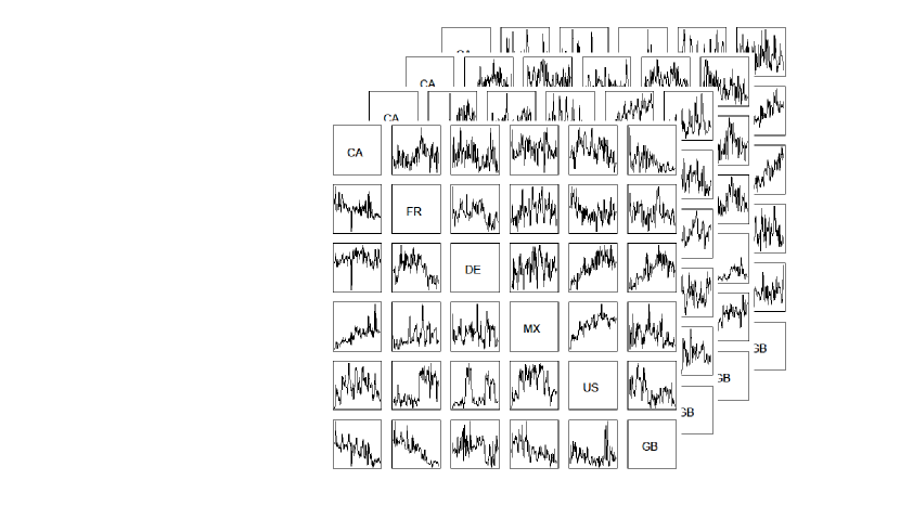
Figure 1: Monthly import-export volume time series of four categories of products (Chemical, Food, Machinery and Electronic, and Footwear and Headwear) among six countries (US, Canada, Mexico, Germany, UK and France) from January 2001 to December 2017.

The import-export network belongs to the general class of dynamic transport (traffic) network. The focus of such a network is the volume of traffic on the links between the nodes on the network. The availability of complex and diverse network data, recorded over periods of time and in very large scales, brings new opportunities with challenges (Aggarwal and Subbian,, 2014). For example, weekly activities in different forms (e.g. text messages, email, phone conversations, and personal interactions) and on different topics (politics, food, travel, photo, emotions, etc) among friends on a social network form a transport network similar to the import-export network, but as a four-dimensional tensor time series. The number of passengers flying between a group of cities with a group of airlines in different classes (economy or business) on different days of the week can be represented as a five-dimensional tensor time series. In Section 7.2 we will present a second example on taxi traffic patterns in New York city. With the city being divided into 69 zones, we study the volume of passenger pickups and drop-offs by taxis among the zones, at different hours during the day as a daily time series of a $69\times 69\times 24$ tensor.

Note that most developed statistical inference methods in network analysis are often confined to static network data such as social network (Goldenberg et al.,, 2010; Snijders,, 2006; Hanneke et al.,, 2010; Kolaczyk and Csárdi,, 2014; Ji and Jin,, 2016; Zhao et al.,, 2012; Phan and Airoldi,, 2015). Of course most networks are dynamic in nature. One important challenge is to develop stochastic models/processes that capture the dynamic dependence and dynamic changes of a network.

Besides dynamic traffic networks, tensor time series are also observed in many other applications. For example, in economics, many economic indicators such as GDP, unemployment rate and inflation index are reported quarterly by many countries, forming a matrix-valued time series. Functional MRI produces a sequence of 3-dimensional brain images (forming 3-dimensional tensors) that changes with different stimulants. Temperature and salinity levels observed at a regular grid of locations and a set of different depth in the ocean form 3-dimensional tensors and are observed over time.

Such tensor systems are often very large. Thirty economic indicators from 30 countries yield total 900 individual time series. Import-export volume of 15 product categories among 20 countries makes up almost 6,000 individual time series. FMRI images often consist of hundreds of thousands of voxels observed over time.

The aim of this paper is to develop a factor model to systematically study the dynamics of tensor systems by jointly modeling the entire tensor simultaneously, while preserving the tensor structure and the time series structure. This is different from the more conventional time series analysis which deals with scalar or vector observations (Box and Jenkins,, 1976; Brockwell and Davis,, 1991; Shumway and Stoffer,, 2002; Tsay,, 2005; Tong,, 1990; Fan and Yao,, 2003; Härdle et al.,, 1997; Tsay and Chen,, 2018) and multivariate time series analysis (Hannan,, 1970; Lütkepohl,, 1993), panel time series analysis (Baltagi,, 2005; Hsiao,, 2003; Geweke,, 1977; Sargent and Sims,, 1977) and spatial-temporal modelling (Bennett,, 1979; Cressie,, 1993; Stein,, 1999; Stroud et al.,, 2001; Woolrich et al.,, 2004; Handcock and Wallis,, 1994; Mardia et al.,, 1998; Wikle and Cressie,, 1999; Wikle et al.,, 1998; Irwin et al.,, 2000).

We mainly focus on the cases when the tensor dimension is large. When dealing with many time series simultaneously, dimension reduction is one of main approaches to extract common information from the data without being overwhelmed by the idiosyncratic variations. One of the most powerful tools for dimension reduction in time series analysis is the dynamic factor model in which ’common’ information is summarized into a small number of factors and the co-movement of the time series is assumed to be driven by these factors and their inherited dynamic structures (Bai,, 2003; Forni et al.,, 2000; Stock and Watson,, 2012; Bai and Ng,, 2008; Connor et al.,, 2012; Chamberlain,, 1983; Peña and Box,, 1987; Pan and Yao,, 2008). We will follow this approach in our development.

The tensor factor model in this paper is similar to the matrix factor model studied in Wang et al., (2019). Specifically, we use a Tucker decomposition type of formation to relate the high-dimensional tensor observations to a low-dimensional latent tensor factor that is assumed to vary over time. Two estimation approaches, named TIPUP and TOPUP, are studied. Asymptotic properties of the estimators are investigated, which provides a comparison between the two estimation methods. The estimation procedure used in Wang et al., (2019) in the matrix setting is essentially the TOPUP procedure. We show that the convergence rate they obtained for the TOPUP can be improved. On the other hand, the TIPUP has a faster rate than the TOPUP, under a mildly more restrictive condition on the level of signal cancellation. The developed theoretical properties also cover the cases where the dimensions of the tensor factor increase with the dimension of the observed tensor time series.

The paper is organized as follows. Section 2 contains some preliminary information on the approach of factor models that we will adopt and the basic notations of tensor analysis. Section 3 introduces a general framework of factor models for large tensor time series, which is assumed to be the sum of a signal part and a noise part. The signal part has a multi-linear factor form, consisting of a low-dimensional tensor that varies over time, and a set of fixed loading matrices in a Tucker decomposition form. Section 4 discusses two general estimation procedures. Their theoretical properties are shown in Section 5. In section 6 we present some simulation studies to demonstrate the performance of the estimation procedures. Two applications are presented in Section 7 to illustrate the model and its interpretations.

2 Preliminary: dynamic factor models and foundation of tensor

In this section we briefly review the linear factor model approach to panel time series data and tensor data analysis. Both serve as a foundation of our approach to tensor time series.

Let $\{(x_{i,t})_{d\times T}\}$ be a set of panel time series. Dynamic factor model assumes

$${\mbox{\boldmath$x$}}_{t}={\mbox{\boldmath$A$}}{\mbox{\boldmath$f$}}_{t}+{\mbox{\boldmath$\mathnormal{\varepsilon}$}}_{t},\mbox{\ or equivelently \ }x_{it}=a_{i1}f_{1t}+\ldots+a_{ir}f_{rt}+\varepsilon_{it}\mbox{\ for }i=1,\ldots,d,$$ (1)

where ${\mbox{\boldmath$f$}}_{t}=(f_{1t},\ldots,f_{rt})^{\top}$ is a set of unobserved latent factor time series with dimension $r\ll d$; The row vector ${\mbox{\boldmath$a$}}_{i}=(a_{i1},\ldots,a_{ir})$, treated as unknown and deterministic, is called factor loading of the $i$-th series. The collection of all ${\mbox{\boldmath$a$}}_{i}$ is called the loading matrix $A$. The idiosyncratic noise ${\mbox{\boldmath$\mathnormal{\varepsilon}$}}_{t}$ is assumed to be uncorrelated with the factors ${\mbox{\boldmath$f$}}_{t}$ in all leads and lags. Both $A$ and ${\mbox{\boldmath$f$}}_{t}$ are unobserved hence some further model assumptions are needed. Two different types of model assumptions are adopted in the literature. One type of models assumes that a common factor must have impact on ‘most’ (defined asymptotically) of the time series, but allows the idiosyncratic noise to have weak cross-correlations and weak autocorrelations (Geweke,, 1977; Sargent and Sims,, 1977; Forni et al.,, 2000; Stock and Watson,, 2012; Bai and Ng,, 2008; Stock and Watson,, 2006; Bai and Ng,, 2002; Hallin and Liška,, 2007; Chamberlain,, 1983; Chamberlain and Rothschild,, 1983; Connor et al.,, 2012; Connor and Linton,, 2007; Fan et al.,, 2016, 2019; Peña and Poncela,, 2006; Bai and Li,, 2012). Under such sets of assumptions, principle component analysis (PCA) of the sample covariance matrix is typically used to estimate the space spanned by the columns of the loading matrix, with various extensions. Another type of models assumes that the factors accommodate all dynamics, making the idiosyncratic noise ‘white’ with no autocorrelation but allowing substantial contemporary cross-correlation among the error process (Peña and Box,, 1987; Pan and Yao,, 2008; Lam et al.,, 2011; Lam and Yao,, 2012; Chang et al.,, 2018). The estimation of the loading space is done by an eigen analysis based on the non-zero lag autocovariance matrices. In this paper we adopt the second approach in our model development.

The key feature of the factor model is that all co-movements of the data are driven by the common factor ${\mbox{\boldmath$f$}}_{t}$ and the factor loading ${\mbox{\boldmath$a$}}_{i}$ provides a link between the underlying factors and the $i$-th series $x_{it}$. This approach has three major benefits: (i) It achieves great reduction in model complexity (i.e. the number of parameters) as the autocovariance matrices are now determined by the loading matrix $A$ and the much smaller autocovariance matrix of the factor process ${\mbox{\boldmath$f$}}_{t}$; (ii) The hidden dynamics (the co-movements) become transparent, leading to clearer and more insightful understanding. This is especially important when the co-movement of the time series is complex and difficult to discover without proper modeling of the full panel; (iii) The estimated factors can be used as input and instrumental variables in models in downstream data analyses, providing summarized and parsimonious information of the whole series.

In the following we briefly review tensor data analysis without involving time series (equivalently at a fixed time point), mainly for the purpose of fixing the notation in our later discussion. For more detailed information, see Kolda and Bader, (2009).

A tensor is a multidimensional array, a generalization of a matrix. The order of a tensor is the number of dimensions, also known as the number of modes. Fibers of a tensor are the higher order analogue of matrix rows and columns, which can be obtained by fixing all but one of the modes. For example, a matrix is a tensor of order $2$, and a matrix column is a mode-1 fiber and a matrix row is a mode-2 fiber.

Consider an order-$K$ tensor ${\cal X}\in\mathbb{R}^{d_{1}\times\cdots\times d_{K}}$. Following Kolda and Bader, (2009), the $k$-mode product of ${\cal X}$ with a matrix ${\mbox{\boldmath$A$}}\in\mathbb{R}^{\tilde{d_{k}}\times d_{k}}$ is an order-$K$ tensor of size $d_{1}\times\cdots\times d_{k-1}\times\tilde{d_{k}}\times d_{k+1}\times...\times d_{K}$ and will be denoted by ${\cal X}\times_{k}{\mbox{\boldmath$A$}}$. Elementwise, $({\cal X}\times_{k}{\mbox{\boldmath$A$}})_{i_{1}\cdots i_{k-1}ji_{k+1}\cdots i_{K}}=\sum_{i_{k}=1}^{d_{k}}x_{i_{1}\cdots i_{k}\cdots i_{K}}a_{ji_{k}}$. Similarly, the $k$-mode product of an order-K tensor with a vector ${\mbox{\boldmath$a$}}\in\mathbb{R}^{d_{k}}$ is an order-$(K-1)$ tensor of size $d_{1}\times...\times d_{k-1}\times d_{k+1}\times...\times d_{K}$ and denoted by ${\cal X}\times_{k}{\mbox{\boldmath$a$}}$. Elementwise, $({\cal X}\times_{k}{\mbox{\boldmath$a$}})_{i_{1}\cdots i_{k-1}i_{k+1}\cdots i_{K}}=\sum_{i_{k}=1}^{d_{k}}x_{i_{1}\cdots i_{k}\cdots i_{K}}a_{i_{k}}$. Let $d=d_{1}\dots d_{K}$ and $d_{-k}=d/d_{k}$. The mode-k unfolding matrix $\hbox{\rm mat}_{k}({\cal X})$ is a $d_{k}\times d_{-k}$ matrix by assembling all $d_{-k}$ mode-k fibers as columns of the matrix. One may also stack a tensor into a vector. Specifically, $\mathrm{vec}({\cal X})$ is a vector in $\mathbb{R}^{d}$ formed by stacking mode-$1$ fibers of ${\cal X}$ in the order of modes $2,\ldots,K$.

The CP decomposition (Carroll and Chang,, 1970; Harshman,, 1970) and Tucker decomposition (Tucker,, 1963, 1964, 1966) are two major extensions of the matrix singular value decomposition (SVD) to tensors of higher order. Recall that the SVD of a matrix ${\mbox{\boldmath$X$}}\in\mathbb{R}^{d_{1}\times d_{2}}$ of rank $r$ has two equivalent forms: ${\mbox{\boldmath$X$}}=\sum_{l=1}^{r}\lambda_{l}{\mbox{\boldmath$u$}}^{(1)}_{l}{\mbox{\boldmath$u$}}_{l}^{(2)\top}$, which decomposes a matrix into a sum of $r$ rank-one matrices, and ${\mbox{\boldmath$X$}}={\mbox{\boldmath$U$}}_{1}{\mbox{\boldmath$\mathnormal{\Lambda}$}}_{r}{\mbox{\boldmath$U$}}_{2}^{\top}$, where ${\mbox{\boldmath$U$}}_{1}$ and ${\mbox{\boldmath$U$}}_{2}$ are orthonormal matrices of size $d_{1}\times r$ and $d_{2}\times r$ spanning the column and row spaces of $X$ respectively, and ${\mbox{\boldmath$\mathnormal{\Lambda}$}}_{r}$ is an $r\times r$ diagonal matrix with $r$ positive singular values on its diagonal. In parallel, CP decomposes an order-$K$ tensor ${\cal X}$ into a sum of rank one tensors, ${\cal X}=\sum_{l=1}^{r}\lambda_{l}{\mbox{\boldmath$u$}}_{l}^{(1)}\otimes{\mbox{\boldmath$u$}}_{l}^{(2)}\otimes\cdots\otimes{\mbox{\boldmath$u$}}_{l}^{(K)}\in\mathbb{R}^{d_{1}\times\cdots\times d_{k}}$, where “$\otimes$” represents the tensor product. The vectors ${{\mbox{\boldmath$u$}}}_{l}^{(k)}\in\mathbb{R}^{d_{k}},l=1,2,...,r$, are not necessarily orthogonal to each other, which differs from the matrix SVD. The Tucker decomposition boils down to $K$ orthonormal matrices ${\mbox{\boldmath$U$}}_{k}\in\mathbb{R}^{d_{k}\times r_{k}}$ containing basis vectors spanning $k$-mode fibers of the tensor, a potentially much smaller ‘core’ tensor ${\cal G}\in\mathbb{R}^{r_{1}\times r_{2}\times\cdots\times r_{K}}$ and the relationship

$${\cal X}={\cal G}\times_{1}{\mbox{\boldmath$U$}}_{1}\times_{2}{\mbox{\boldmath$U$}}_{2}\times_{3}\cdots\times_{K}{\mbox{\boldmath$U$}}_{K}={\cal G}\times_{k=1}^{K}{\mbox{\boldmath$U$}}_{k}.$$ (2)

Note that the core tensor ${\cal G}$ is similar to the ${\mbox{\boldmath$\mathnormal{\Lambda}$}}_{r}$ in the middle of matrix SVD but now it is not necessarily diagonal.

3 A Tensor Factor Model

In tensor times series, the observed tensors would depend on $t=1,\ldots,T$ and be denoted by ${\cal X}_{t}\in\mathbb{R}^{d_{1}\times\cdots\times d_{K}}$ as a series of order-$K$ tensors. By absorbing time, we may stack ${\cal X}_{t}$ into an order-$(K+1)$ tensor ${\cal Y}\in\mathbb{R}^{d_{1}\times\cdots\times d_{K}\times T}$, with time $t$ as the $(K+1)$-th mode, referred to as the time-mode. We assume the following decomposition

$${\cal Y}={\cal S}+{\cal R},\mbox{\ \ or equivalently \ \ }{\cal X}_{t}={\cal M}_{t}+{\cal E}_{t},$$ (3)

where ${\cal S}$ is the dynamic signal component and ${\cal R}$ is a white noise part. In the second expression (3), ${\cal M}_{t}$ and ${\cal E}_{t}$ are the corresponding signal and noise components of ${\cal X}_{t}$, respectively. We assume that the noise ${\cal E}_{t}$ are uncorrelated (white) across time, following Lam and Yao, (2012).

In this model, all dynamics are contained in the signal component ${\cal M}_{t}$. We assume that ${\cal M}_{t}$ is in a lower-dimensional space and has certain multilinear decomposition. We further assume that any component in this multilinear decomposition that involves the time-mode is random and dynamic, and will be called a factor component (depending on its order, it will be called a scalar factor $f_{t}$, a vector factor ${\mbox{\boldmath$f$}}_{t}$, a matrix factor ${\mbox{\boldmath$F$}}_{t}$, or a tensor factor ${\cal F}_{t}$), which when concatenated along the time-mode forms a higher order object, such as ${\mbox{\boldmath$g$}},{\mbox{\boldmath$G$}},{\cal G}$. Any components of ${\cal M}_{t}$ other than ${\cal F}_{t}$ are assumed to be deterministic and will be called the loading components.

Although it is tempting to directly model ${\cal S}$ with standard tensor decomposition approaches to find its lower dimensional structure, the dynamics and dependency in the time direction (auto-dependency) are important and should be treated differently. Traditional tensor decomposition using tensor SVD/PCA on ${\cal S}$ ignores the special role of the time-mode and the covariance structure in the time direction, and treats the signal ${\cal S}$ as deterministic (Richard and Montanari,, 2014; Anandkumar et al.,, 2014; Hopkins et al.,, 2015; Sun et al.,, 2016). Such a direct approach often leads to inferior inference results as our preliminary results have demonstrated (Wang et al.,, 2019). In our approach, the component in the time direction is considered as latent and random. As a result, our model assumptions and interpretations, and their corresponding estimation procedures and theoretical properties are significantly different.

In the following we propose a specific model for tensor time series, based on a decomposition similar to Tucker decomposition. Specifically, we assume that

$${\cal S}={\cal G}\times_{1}{\mbox{\boldmath$A$}}_{1}\times_{2}\ldots\times_{K}{\mbox{\boldmath$A$}}_{K}\mbox{ \ or equivalently \ }{\cal M}_{t}={\cal F}_{t}\times_{1}{\mbox{\boldmath$A$}}_{1}\times_{2}\ldots\times_{K}{\mbox{\boldmath$A$}}_{K}$$ (4)

where ${\cal F}_{t}$ is itself a tensor times series of dimension $r_{1}\times\ldots\times r_{K}$ with small $r_{k}\ll d_{k}$ and ${\mbox{\boldmath$A$}}_{k}$ are $d_{k}\times r_{k}$ loading matrices. We assume without loss of generality in the sequel that ${\mbox{\boldmath$A$}}_{k}$ is of rank $r_{k}$.

Model (4) resembles a Tucker-type decomposition similar to (2) where the core tensor ${\cal G}\in\mathbb{R}^{r_{1}\times\ldots\times r_{K}\times T}$ is the factor term and the loading matrices ${\mbox{\boldmath$A$}}_{k}\in\mathbb{R}^{d_{k}\times r_{k}}$ are constant matrices, whose column spaces are identifiable. The core tensor ${\cal F}_{t}$ is usually much smaller than ${\cal X}_{t}$ in dimension. It drives all the comovements of individual time series in ${\cal X}_{t}$. For matrix time series, model (4) becomes ${\mbox{\boldmath$M$}}_{t}={\mbox{\boldmath$F$}}_{t}\times_{1}{\mbox{\boldmath$A$}}_{1}\times_{2}{\mbox{\boldmath$A$}}_{2}={\mbox{\boldmath$A$}}_{1}{\mbox{\boldmath$F$}}_{t}{\mbox{\boldmath$A$}}_{2}^{\top}$. The matrix version of Model (4) was considered in Wang et al., (2019), which also provided several model interpretations. Most of their interpretations can be extended to the tensor factor model. In this paper we consider more general model settings and more powerful estimation procedures.

As ${\cal F}_{t}\to{\cal X}_{t}={\cal F}_{t}{\times_{k=1}^{K}{\mbox{\boldmath$A$}}_{k}}+{\cal E}_{t}$ is a linear mapping from $\mathbb{R}^{r_{1}\times\cdots\times r_{K}}$ to $\mathbb{R}^{d_{1}\times\cdots\times d_{K}}$. It can be written as a matrix acting on vectors as in

$$\mathrm{vec}({\cal X}_{t})={\rm Kronecker}\left({\mbox{\boldmath$A$}}_{K},\ldots,{\mbox{\boldmath$A$}}_{1}\right)\mathrm{vec}({\cal F}_{t})+\mathrm{vec}({\cal E}_{t}),$$

where ${\rm Kronecker}\left({\mbox{\boldmath$A$}}_{K},\ldots,{\mbox{\boldmath$A$}}_{1}\right)\in\mathbb{R}^{d\times r}$ is the Kronecker product, $d=\prod_{k=1}^{K}d_{k}$, $r=\prod_{k=1}^{K}r_{k}$, and $\mathrm{vec}(\cdot)$ is the tensor stacking operator as described in Section 2. While $\otimes$ is often used to denote the Kronecker product, we shall avoid this usage as $\otimes$ is preserved to denote the tensor product in this paper. For example, in the case of $K=2$ with observation ${\mbox{\boldmath$X$}}_{t}\in\mathbb{R}^{d_{1}\times d_{2}}$, ${\mbox{\boldmath$X$}}_{t-h}\otimes{\mbox{\boldmath$X$}}_{t}$ is a $d_{1}\times d_{2}\times d_{1}\times d_{2}$ tensor of order four, not a matrix of dimension $d_{1}^{2}\times d_{2}^{2}$, as we would need to consider the model-2 unfolding of ${\mbox{\boldmath$X$}}_{t-h}\otimes{\mbox{\boldmath$X$}}_{t}$ as a $d_{2}\times(d_{1}^{2}d_{2})$ matrix. The Kronecker expression exhibits the same form as in the factor model for panel time series except that the loading matrix of size $d\times r$ in the vector factor model is assumed to have a Kronecker product structure of $K$ matrices of much smaller sizes $d_{i}\times r_{i}$ ($i=1,\ldots,K$). Hence the tensor factor model reduces the number of parameters in the loading matrices from $dr=d_{1}r_{1}\ldots d_{K}r_{K}$ in the stacked vector version to $d_{1}r_{1}+\ldots+d_{K}r_{K}$, a very significant dimension reduction. The dimension reduction comes from the assumption imposed on the loading matrices.

It would be tempting to assume the orthonormality of ${\mbox{\boldmath$A$}}_{k}\in\mathbb{R}^{d_{k}\times r_{k}}$ as in SVD and Tucker decomposition. However, in the high-dimensional setting, this may not be compatible in general with the assumption that ${\cal F}_{t}$ is a “regular” factor series with unit order of magnitude, which we may also want to impose; The magnitude of ${\cal X}_{t}$ would have to be absorbed into either ${\cal F}_{t}$ or $\{{\mbox{\boldmath$A$}}_{k}\}$ in model (4). In addition, the orthonormality of ${\mbox{\boldmath$A$}}_{k}$ would be incompatible with the expression of the strength of the factor in terms of the norm of ${\mbox{\boldmath$A$}}_{k}$ as in the literature (Bai and Ng,, 2008; Lam and Yao,, 2012; Wang et al.,, 2019). Thus, we shall consider general ${\mbox{\boldmath$A$}}_{k}$ to preserve flexibility.

Let ${\mbox{\boldmath$A$}}_{k}={\mbox{\boldmath$U$}}_{k}{\mbox{\boldmath$\mathnormal{\Lambda}$}}_{k}{\mbox{\boldmath$V$}}_{k}^{\top}$ be the SVD of ${\mbox{\boldmath$A$}}_{k}$. The tensor time series in (4) can be then written as ${\cal X}_{t}=\big{(}{\cal F}_{t}\times_{k=1}^{K}({\mbox{\boldmath$\mathnormal{\Lambda}$}}_{k}{\mbox{\boldmath$V$}}_{k}^{\top})\big{)}\times_{k=1}^{K}{\mbox{\boldmath$U$}}_{k}$. In the special case where the $r_{1}\times\cdots\times r_{K}$ dimensional series $\big{(}{\cal F}_{t}\times_{k=1}^{K}({\mbox{\boldmath$\mathnormal{\Lambda}$}}_{k}{\mbox{\boldmath$V$}}_{k}^{\top})\big{)}/{\lambda}$ can be viewed as a properly normalized factor for some signal strength parameter ${\lambda}>0$, we may absorb ${\mbox{\boldmath$\mathnormal{\Lambda}$}}_{k}$, ${\mbox{\boldmath$V$}}_{k}^{\top}$ and $1/{\lambda}$ into ${\cal F}_{t}$ and write (4) as

$${\cal X}_{t}={\lambda}\big{(}{\cal F}_{t}\times_{1}{\mbox{\boldmath$U$}}_{1}\times_{2}\cdots\times_{K}{\mbox{\boldmath$U$}}_{k}\big{)}+{\cal E}_{t}$$ (5)

with orthonormal ${\mbox{\boldmath$U$}}_{k}\in\mathbb{R}^{d_{k}\times r_{k}}$ and properly normalized ${\cal F}_{t}$. This means ${\mbox{\boldmath$A$}}_{k}=c_{k}{\mbox{\boldmath$U$}}_{k}$ in (4) with constants $c_{k}$ and ${\lambda}=\prod_{k=1}^{K}c_{k}$. For example, in the one-factor model where $r_{1}=\cdots=r_{K}=1$, ${\cal X}_{t}=\big{(}{\lambda}f_{t}\big{)}{\mbox{\boldmath$u$}}_{1}\otimes\cdots\otimes{\mbox{\boldmath$u$}}_{K}$ as in (46) would be discussed in detail below Theorems 1 and 2.

Remark:  In our theoretical development, we do not impose any specific structure for the dynamics of the relatively low-dimensional factor process ${\cal F}_{t}\in\mathbb{R}^{r_{1}\times\cdots\times r_{K}}$, except conditions on the spectrum norm and singular values of certain matrices in the unfolding of the average of the cross-product $(T-h)^{-1}(\sum_{t=h+1}^{T}{\cal M}_{t-h}\otimes{\cal M}_{t})$. As ${\cal M}_{t}={\cal F}_{t}\times_{k=1}^{K}{\mbox{\boldmath$A$}}_{k}$, these conditions on ${\cal M}_{t}$ would hold when the condition numbers of ${\mbox{\boldmath$A$}}_{k}^{\top}{\mbox{\boldmath$A$}}_{k}$ are bounded, e.g. model (5), and parallel conditions on the spectrum norm and singular values in the unfolding of $(T-h)^{-1}\sum_{t=h+1}^{T}{\cal F}_{t-h}\otimes{\cal F}_{t}$ hold through the consistency of the averages. For fixed $r_{1},\ldots,r_{k}$, such consistency for the low-dimensional ${\cal F}_{t}$ has been extensively studied in the literature with many options such as various mixing conditions.

Remark:  The above tensor factor model does not assume any structure on the noises except that the noise process is white. The estimation procedures we use do not require any additional structure. But in many cases it benefits to allow specific structures for the contemporary cross-correlation of the elements of ${\cal E}_{t}$. For example, one may assume ${\cal E}_{t}={\cal Z}_{t}\times_{1}{\mbox{\boldmath$\mathnormal{\Sigma}$}}_{1}^{1/2}\times_{2}{\mbox{\boldmath$\mathnormal{\Sigma}$}}_{2}^{1/2}\times_{3}\ldots\times_{K}{\mbox{\boldmath$\mathnormal{\Sigma}$}}_{K}^{1/2}$ where all elements in ${\cal Z}_{t}$ are i.i.d. $N(0,1)$. Hence each of the ${\mbox{\boldmath$\mathnormal{\Sigma}$}}_{i}$ can be viewed as the common covariance matrix of mode-$i$ fiber in the tensor ${\cal E}_{t}$. More efficient estimators may be constructed to utilize such a structure but is out of the scope of this paper.

4 Estimation procedures

Low-rank tensor approximation is a delicate task. To begin with, the best rank-$r$ approximation to a tensor may not exist (de Silva and Lim,, 2008) or NP hard to compute (Hillar and Lim,, 2013). On the other hand, despite such inherent difficulties, many heuristic techniques are widely used and often enjoy great successes in practice. Richard and Montanari, (2014) and Hopkins et al., (2015), among others, have considered a rank-one spiked tensor model ${\cal S}+{\cal R}$ as a vehicle to investigate the requirement of signal-to-noise ratio for consistent estimation under different constraints of computational resources, where ${\cal S}={\lambda}{\mbox{\boldmath$u$}}_{1}\otimes{\mbox{\boldmath$u$}}_{2}\otimes{\mbox{\boldmath$u$}}_{3}$ for some deterministic unit vectors ${\mbox{\boldmath$u$}}_{k}\in\mathbb{R}^{d_{k}}$ and all entries of ${\cal R}$ are iid standard normal. As shown by Richard and Montanari, (2014), in the symmetric case where $d_{1}=d_{2}=d_{3}=d$, ${\cal S}$ can be estimated consistently by the MLE when $\sqrt{d}/\lambda=o(1)$. Similar to the case of spiked PCA (Koltchinskii et al.,, 2011; Negahban and Wainwright,, 2011), it can be shown that the rate achieved by the MLE is minimax among all estimators when ${\cal S}$ is treated as deterministic. However, at the same time it is also unsatisfactory as the MLE of ${\cal S}$ is NP hard to compute even in this simplest rank one case. Additional discussion of this and some other key differences between matrix and tensor estimations can be found in recent studies of related tensor completion problems (Barak and Moitra,, 2016; Yuan and Zhang,, 2016, 2017; Xia and Yuan,, 2017; Zhang et al.,, 2019).

A commonly used heuristic to overcome this computational difficulty is tensor unfolding. In the following we proposed two estimation methods that are based on a marriage of tensor unfolding and the use of lagged cross-product, the tensor version of the autocovariance. This is due to the dynamic and random nature of the latent factor process, and the whiteness assumption on the error process.

As in all factor models, due to ambiguity, we will only estimate the linear spaces spanned by the loading matrices with an orthonormal representation of the loading spaces, or equivalently, only estimate the orthogonal projection matrix to such spaces.

The lagged cross-product operator, which we denote by ${\mbox{\boldmath$\mathnormal{\Sigma}$}}_{h}$, can be viewed as the $(2K)$-tensor

$${\mbox{\boldmath$\mathnormal{\Sigma}$}}_{h}=\mathbb{E}\bigg{[}\sum_{t=h+1}^{T}\frac{{\cal X}_{t-h}\otimes{\cal X}_{t}}{T-h}\bigg{]}=\mathbb{E}\bigg{[}\sum_{t=h+1}^{T}\frac{{\cal M}_{t-h}\otimes{\cal M}_{t}}{T-h}\bigg{]}\in\mathbb{R}^{{d_{1}\times\cdots\times d_{K}}\times{d_{1}\times\cdots\times d_{K}}},$$

$h=1,\ldots,h_{0}$. We consider two estimation methods based on the sample version of ${\mbox{\boldmath$\mathnormal{\Sigma}$}}_{h}$,

$${\overline{\mbox{\boldmath$\mathnormal{\Sigma}$}}}_{h}=\sum_{t=h+1}^{T}\frac{{\cal X}_{t-h}\otimes{\cal X}_{t}}{T-h},\quad h=1,\ldots,h_{0}.$$ (6)

The orthogonal projection to the column space of ${\mbox{\boldmath$A$}}_{k}$ is

$${\mbox{\boldmath$P$}}_{k}={\mbox{\boldmath$A$}}_{k}\big{(}{\mbox{\boldmath$A$}}_{k}^{\top}{\mbox{\boldmath$A$}}_{k}\big{)}^{-1}{\mbox{\boldmath$A$}}_{k}^{\top}.$$ (7)

It is the $k$-th principle space of the tensor time series ${\cal M}_{t}={\cal F}_{t}{\times_{k=1}^{K}{\mbox{\boldmath$A$}}_{k}}$ in (4). As ${\cal M}_{t}={\cal M}_{t}{\times_{k=1}^{K}{\mbox{\boldmath$P$}}_{k}}$ for all $t$,

$${{\mbox{\boldmath$\mathnormal{\Sigma}$}}}_{h}={{\mbox{\boldmath$\mathnormal{\Sigma}$}}}_{h}{\times_{k=1}^{2K}{\mbox{\boldmath$P$}}_{k}}=\mathbb{E}\bigg{[}\sum_{t=h+1}^{T}\frac{{\cal F}_{t-h}\otimes{\cal F}_{t}}{T-h}\bigg{]}{\times_{k=1}^{2K}{{\mbox{\boldmath$P$}}_{k}{\mbox{\boldmath$A$}}_{k}}}.$$

with the notation ${\mbox{\boldmath$A$}}_{k}={\mbox{\boldmath$A$}}_{k-K}$ and ${\mbox{\boldmath$P$}}_{k}={\mbox{\boldmath$P$}}_{k-K}$ for $k>K$. Once consistent estimates $\widehat{{\mbox{\boldmath$P$}}_{k}}$ are obtained for ${\mbox{\boldmath$P$}}_{k}$, the estimation of other aspects of ${{\mbox{\boldmath$\mathnormal{\Sigma}$}}}_{h}$ can be carried out based on the low-rank projection of (6),

$${\overline{\mbox{\boldmath$\mathnormal{\Sigma}$}}}_{h}{\times_{k=1}^{2K}{\widehat{{\mbox{\boldmath$P$}}_{k}}}}=\sum_{t=h+1}^{T}\frac{({\cal X}_{t-h}{\times_{k=1}^{K}{\widehat{{\mbox{\boldmath$P$}}_{k}}}})\otimes({\cal X}_{t}{\times_{k=1}^{K}{\widehat{{\mbox{\boldmath$P$}}_{k}}}})}{T-h},$$

as if the low-rank tensor time series ${\cal X}_{t}{\times_{k=1}^{K}{\widehat{{\mbox{\boldmath$P$}}_{k}}}}$ is observed. For the estimation of ${\mbox{\boldmath$P$}}_{k}$, we propose two methods, and both methods can be written in terms of the mode-$k$ matrix unfolding $\hbox{\rm mat}_{k}({\cal X}_{t})$ of ${\cal X}_{t}$ as follows.

(i) TOPUP method: We define a order-5 tensor as

$${\rm TOPUP}_{k}=\bigg{(}\sum_{t=h+1}^{T}\frac{\hbox{\rm mat}_{k}({\cal X}_{t-h})\otimes\hbox{\rm mat}_{k}({\cal X}_{t})}{T-h},h=1,\ldots,h_{0}\bigg{)}$$ (8)

where $\otimes$ is the tensor product and $h$ is the index for the 5-th mode. Let $d_{-k}=d/d_{k}$ with $d=\prod_{k=1}^{K}d_{k}$. As $\hbox{\rm mat}_{k}({\cal X}_{t})$ is a $d_{k}\times d_{-k}$ matrix, ${\rm TOPUP}_{k}$ is of dimension $d_{k}\times d_{-k}\times d_{k}\times d_{-k}\times h_{0}$, so that $\hbox{\rm mat}_{1}\big{(}{\rm TOPUP}_{k}\big{)}$ is a $d_{k}\times(d^{2}h_{0}/d_{k})$ matrix. Let

$$\widehat{{\mbox{\boldmath$P$}}_{k,m}}=\hbox{\rm PLSVD${}_{m}$}\Big{(}\hbox{\rm mat}_{1}\Big{(}{\rm TOPUP}_{k}\Big{)}\Big{)},$$ (9)

where PLSVD_m stands for the orthogonal projection to the span of the first $m$ left singular vectors of a matrix. We estimate the projection $\widehat{{\mbox{\boldmath$P$}}_{k}}$ by $\widehat{{\mbox{\boldmath$P$}}_{k,\widehat{r_{k}}}}$ with a proper $\widehat{r_{k}}$. When $r_{k}$ is given,

$$\widehat{{\mbox{\boldmath$P$}}_{k}}=\widehat{{\mbox{\boldmath$P$}}_{k,r_{k}}}.$$

The above method is expected to yield consistent estimates of ${\mbox{\boldmath$P$}}_{k}$ under proper conditions on the dimensionality, signal strength and noise level since (8) and (4) imply

$$\mathbb{E}\Big{[}\hbox{\rm mat}_{1}\Big{(}{\rm TOPUP}_{k}\Big{)}\Big{]}$$ (10)

$$= \hbox{\rm mat}_{1}\Big{(}\hbox{$\sum_{t=h+1}^{T}$}\mathbb{E}\big{(}\hbox{\rm mat}_{k}({\cal M}_{t-h})\otimes\hbox{\rm mat}_{k}({\cal M}_{t})\big{)}/(T-h),h=1,\ldots,h_{0}\Big{)}$$ (11)

$$= \hbox{\rm mat}_{k}\Big{(}\Big{\{}\hbox{$\sum_{t=h+1}^{T}$}\mathbb{E}\big{(}{\cal F}_{t-h}\otimes{\cal F}_{t}\big{)}/(T-h)\Big{\}}{\times_{k=1}^{2K}{\mbox{\boldmath$A$}}_{k}},h=1,\ldots,h_{0}\Big{)}$$ (12)

$$= {\mbox{\boldmath$A$}}_{k}\hbox{\rm mat}_{k}\Big{(}\hbox{$\sum_{t=h+1}^{T}$}\mathbb{E}\big{(}{\cal F}_{t-h}\otimes{\cal F}_{t}\big{)}/(T-h)\Big{\}}\times_{\ell=1}^{k-1}{\mbox{\boldmath$A$}}_{\ell}\times_{\ell=k+1}^{2K}{\mbox{\boldmath$A$}}_{\ell},h=1,\ldots,h_{0}\Big{)}.$$ (13)

This is a product of two matrices, with ${\mbox{\boldmath$A$}}_{k}={\mbox{\boldmath$P$}}_{k}{\mbox{\boldmath$A$}}_{k}$ on the left.

We note that the left singular vectors of $\hbox{\rm mat}_{1}\big{(}{\rm TOPUP}_{k}\big{)}$ are the same as the eigenvectors in the PCA of the $d_{k}\times d_{k}$ nonnegative-definite matrix

$$\widehat{{\mbox{\boldmath$W$}}}_{k}=\hbox{\rm mat}_{1}\Big{(}{\rm TOPUP}_{k}\Big{)}\hbox{\rm mat}_{1}^{\top}\Big{(}{\rm TOPUP}_{k}\Big{)},$$ (14)

which can be viewed as the sample version of

$${\mbox{\boldmath$W$}}_{k}=\hbox{\rm mat}_{1}\big{(}\mathbb{E}\big{(}{\rm TOPUP}_{k}\big{)}\big{)}\hbox{\rm mat}_{1}^{\top}\big{(}\mathbb{E}\big{(}{\rm TOPUP}_{k}\big{)}\big{)}.$$ (15)

It follows from (10) that ${\mbox{\boldmath$W$}}_{k}$ has a sandwich formula with ${\mbox{\boldmath$A$}}_{k}$ on the left and ${\mbox{\boldmath$A$}}_{k}^{\top}$ on the right.

As ${\mbox{\boldmath$A$}}_{k}$ is assumed to be of rank $r_{k}$, its column space is identical to that of $\mathbb{E}\big{[}\hbox{\rm mat}_{1}\big{(}{\rm TOPUP}_{k}\big{)}\big{]}$ in (10) or that of ${\mbox{\boldmath$W$}}_{k}$ in (15) as long as they are also of rank $r_{k}$. Thus ${\mbox{\boldmath$P$}}_{k}$ is identifiable from the population version of TOPUP_k. However, further identification of the lagged cross-product operator by the TOPUP would involve parameters specific to the TOPUP approach. For example, if we write ${\mbox{\boldmath$P$}}_{k}={\mbox{\boldmath$U$}}_{k}{\mbox{\boldmath$U$}}_{k}^{\top}$ where ${\mbox{\boldmath$U$}}_{k}=({\mbox{\boldmath$u$}}_{k,1},\ldots,{\mbox{\boldmath$u$}}_{k,r_{k}})$ is orthonormal, the TOPUP estimator (9) is designed to estimate $({\mbox{\boldmath$u$}}_{k,1},\ldots,{\mbox{\boldmath$u$}}_{k,m})$ as the left singular matrix of $\mathbb{E}\big{[}\hbox{\rm mat}_{1}\big{(}{\rm TOPUP}_{k}\big{)}\big{]}$. Even then, the singular vector ${\mbox{\boldmath$u$}}_{k,m}$ is identifiable only up to the sign through the projections ${\mbox{\boldmath$P$}}_{k,m}=\sum_{j=1}^{m}{\mbox{\boldmath$u$}}_{k,j}{\mbox{\boldmath$u$}}_{k,j}^{\top}$ and ${\mbox{\boldmath$P$}}_{k,m-1}$ provided a sufficiently large gap between the $(m-1)$-th, the $m$-th and the $(m+1)$-th singular values of the matrix relative to the TOPUP estimation error.

For the ease of discussion, we consider for example the case of $k=1$ and $K=3$ with stationary factor ${\cal F}_{t}$ where ${\cal X}_{t}\in\mathbb{R}^{d_{1}\times d_{2}\times d_{3}}$ is a 3-way tensor, and its lag-$h$ ($h>0$) autocovariance ${\mbox{\boldmath$\mathnormal{\Sigma}$}}_{h}$ is a 6-way tensor with dimensions $d_{1}\times d_{2}\times d_{3}\times d_{1}\times d_{2}\times d_{3}$ and elements $\sigma^{(h)}_{i_{1},j_{1},k_{1},i_{2},j_{2},k_{2}}=cov(x_{i_{1}j_{1}k_{1},t-h},x_{i_{2}j_{2}k_{2},t})$. For the estimation of the column space of the loading matrix ${\mbox{\boldmath$A$}}_{1}$, we write

$${\mbox{\boldmath$W$}}_{1} = \sum_{h=1}^{h_{0}}\,\sum_{j_{1},k_{1}}\,\sum_{i_{2},j_{2},k_{2}}\Big{(}\mathbb{E}\Big{[}{\mbox{\boldmath$x$}}_{\cdot,j_{1},k_{1},t-h}^{(1)}x_{i_{2},j_{2},k_{2},t}\Big{]}\Big{)}\Big{(}\mathbb{E}\Big{[}{\mbox{\boldmath$x$}}_{\cdot,j_{1},k_{1},t-h}^{(1)}x_{i_{2},j_{2},k_{2},t}\Big{]}\Big{)}^{\top}$$ (16)

$$= \sum_{h=1}^{h_{0}}\,\sum_{j_{1},k_{1}}\,\sum_{j_{2},k_{2}}\Big{(}\mathbb{E}\Big{[}{\mbox{\boldmath$x$}}_{\cdot,j_{1},k_{1},t-h}{\mbox{\boldmath$x$}}_{\cdot,j_{2},k_{2},t}^{\top}\Big{]}\Big{)}\Big{(}\mathbb{E}\Big{[}{\mbox{\boldmath$x$}}_{\cdot,j_{1},k_{1},t-h}{\mbox{\boldmath$x$}}_{\cdot,j_{2},k_{2},t}^{\top}\Big{]}\Big{)}^{\top}$$

$$= {\mbox{\boldmath$A$}}_{1}\bigg{(}\sum_{h=1}^{h_{0}}\,\sum_{j_{1},k_{1}}\,\sum_{j_{2},k_{2}}{\mbox{\boldmath$\mathnormal{\Gamma}$}}_{j_{1},k_{1},j_{2},k_{2},h}{\mbox{\boldmath$\mathnormal{\Gamma}$}}_{j_{1},k_{1},j_{2},k_{2},h}^{\top}\bigg{)}{\mbox{\boldmath$A$}}_{1}^{\top}$$

in view of (15), where ${\mbox{\boldmath$\mathnormal{\Gamma}$}}_{j_{1},k_{1},j_{2},k_{2},h}=\rm{cov}({\cal F}_{t-h},{\cal F}_{t})\times_{2}{\mbox{\boldmath$A$}}_{2,j_{1}\cdot}\times_{3}{\mbox{\boldmath$A$}}_{3,k_{1}\cdot}\times_{4}{\mbox{\boldmath$A$}}_{1}\times_{5}{\mbox{\boldmath$A$}}_{2,j_{2}\cdot}\times_{6}{\mbox{\boldmath$A$}}_{3,k_{2}\cdot}\in\mathbb{R}^{r_{1}\times d_{1}}$. This is a non-negative definite matrix sandwiched by ${\mbox{\boldmath$A$}}_{1}$ and ${\mbox{\boldmath$A$}}_{1}^{\top}$. Hence the column space of ${\mbox{\boldmath$A$}}_{1}$ and the column space of ${{\mbox{\boldmath$W$}}_{1}}$ are the same, if the matrix between ${\mbox{\boldmath$A$}}_{1}$ and ${\mbox{\boldmath$A$}}_{1}^{\top}$ in (16) is of full rank.

The TOPUP can be then described in terms of the PCA as follows. Replacing ${{\mbox{\boldmath$W$}}_{1}}$ with its sample version ${\widehat{{\mbox{\boldmath$W$}}}_{1}}$ and through eigenvalue decomposition, we can estimate the top $r_{k}$-eigenvectors of ${\widehat{{\mbox{\boldmath$W$}}}_{1}}$, which form a representative of the estimated space spanned by ${\mbox{\boldmath$A$}}_{1}$. Representative sets of eigenvectors of ${\mbox{\boldmath$A$}}_{2}$ and ${\mbox{\boldmath$A$}}_{3}$ can be obtained similarly. This procedure uses the outer-product of all (time shifted) mode-1 fibers of the observed tensor ${\cal Y}\in\mathbb{R}^{d_{1}\times d_{2}\times d_{3}\times T}$. Then, after taking the squares, it sums over the other modes. By considering positive lags $h>0$, we explicitly utilize the assumption that the noise process is white, hence avoiding having to deal with the contemporary covariance structure of ${\cal E}_{t}$, as it disappears in ${\mbox{\boldmath$\mathnormal{\Gamma}$}}_{j_{1},k_{1},j_{2},k_{2},h}$ for all $h>0$. We also note that while the PCA of $\widehat{{\mbox{\boldmath$W$}}}_{k}$ in (14) is equivalent to the SVD in (9) for the estimation of ${\mbox{\boldmath$P$}}_{k}$, it can be computationally more efficient to perform the SVD directly in many cases.

We call this TOPUP (Time series Outer-Product Unfolding Procedure) as the tensor product in the matrix unfolding in (8) is a direct extension of the vector outer product, which is actually used in the equivalent formulation in (16). This reduces to the algorithm in Wang et al., (2019) for matrix time series.

(ii) TIPUP method: The TIPUP (Time series Inner-Product Unfolding Procedure) can be simply described as the replacement of the tensor product in (8) with the inner product:

$${\rm TIPUP}_{k}=\bigg{(}\sum_{t=h+1}^{T}\frac{\hbox{\rm mat}_{k}({\cal X}_{t-h})\hbox{\rm mat}_{k}^{\top}({\cal X}_{t})}{T-h},h=1,\ldots,h_{0}\bigg{)},$$ (17)

which is treated as a matrix of dimension $d_{k}\times(d_{k}h_{0})$. The estimator $\widehat{{\mbox{\boldmath$P$}}_{k,m}}$ is then defined as

$$\widehat{{\mbox{\boldmath$P$}}_{k,m}}=\hbox{\rm PLSVD${}_{m}$}\big{(}{\rm TIPUP}_{k}\big{)}.$$ (18)

Again TIPUP is expected to yield consistent estimates of ${\mbox{\boldmath$P$}}_{k}$ in (7) as

$$\mathbb{E}\big{[}{\rm TIPUP}_{k}\big{]}$$ (19)

$$= \Big{(}\big{\langle}{\mbox{\boldmath$\mathnormal{\Sigma}$}}_{h},{\mbox{\boldmath$I$}}_{k,k+K}\big{\rangle}_{\{k,k+K\}^{c}},h=1,\ldots,h_{0}\Big{)}$$

$$= {\mbox{\boldmath$A$}}_{k}{\Big{(}}\big{\langle}\mathbb{E}\big{[}\hbox{$\sum_{t=h+1}^{T}$}({\cal F}_{t-h}\otimes{\cal F}_{t})/(T-h)\big{]}\times_{\ell\neq k,1\leq\ell\leq 2K}{\mbox{\boldmath$A$}}_{\ell},{\mbox{\boldmath$I$}}_{k,k+K}\big{\rangle}_{\{k,k+K\}^{c}},h\leq h_{0}\Big{)},$$

where ${\mbox{\boldmath$I$}}_{k,k+K}$ is the $(2K)$-tensor with elements $({\mbox{\boldmath$I$}}_{k,k+K})_{{\mbox{\boldmath$i$}},{\mbox{\boldmath$j$}}}=I\{{\mbox{\boldmath$i$}}_{-k}={\mbox{\boldmath$j$}}_{-k}\}$ at ${\mbox{\boldmath$i$}}=(i_{1},\ldots,i_{K})$ and ${\mbox{\boldmath$j$}}=\{j_{1},\ldots,j_{K})$, and $\langle\cdot,\cdot\rangle_{\{k,k+K\}^{c}}$ is the inner product summing over indices other than $\{k,k+K\}$.

We use the superscript ^∗ to indicate the TIPUP counterpart of TOPUP quantities, e.g.

$$\widehat{{\mbox{\boldmath$W$}}}_{k}^{*}=\big{(}{{\rm TIPUP}_{k}}\big{)}\big{(}{{\rm TIPUP}_{k}}\big{)}^{\top}$$ (21)

is the sample version of

$${\mbox{\boldmath$W$}}_{k}^{*}=\mathbb{E}\big{[}{\rm TIPUP}_{k}\big{]}\mathbb{E}\big{[}{\rm TIPUP}_{k}^{\top}\big{]}.$$ (22)

We note that by (19) ${\mbox{\boldmath$W$}}_{k}^{*}$ is again sandwiched between ${\mbox{\boldmath$A$}}_{k}$ and ${\mbox{\boldmath$A$}}_{k}^{\top}$. For $k=1$ and $K=3$,

$${\mbox{\boldmath$W$}}_{1}^{*}={\mbox{\boldmath$A$}}_{1}\left[\sum_{h=1}^{h_{0}}\left(\sum_{j,k}{\mbox{\boldmath$\mathnormal{\Gamma}$}}_{j,k,j,k,h}\right)\left(\sum_{j,k}{\mbox{\boldmath$\mathnormal{\Gamma}$}}_{j,k,j,k,h}\right)^{\top}\right]{\mbox{\boldmath$A$}}_{1}^{\top}$$ (23)

with ${\mbox{\boldmath$\mathnormal{\Gamma}$}}_{j_{1},k_{1},j_{2},k_{2},h}$ being that in (16). If the middle term in (23) is of full rank, then the column space of ${\mbox{\boldmath$W$}}_{1}^{*}$ is the same as that of ${\mbox{\boldmath$A$}}_{1}$.

As in the case of the TOPUP, for the estimation of the auto-covariance operator beyond ${\mbox{\boldmath$P$}}_{k}$, the TIPUP would only identify parameters specific to the approach. For example, the TIPUP estimator (18) aims to estimate ${\mbox{\boldmath$P$}}^{*}_{k,m}=\sum_{j=1}^{m}{\mbox{\boldmath$u$}}_{k,j}^{*}({\mbox{\boldmath$u$}}_{k,j}^{*})^{\top}$ with ${\mbox{\boldmath$U$}}_{k}^{*}$ being the left singular matrix of $\mathbb{E}\big{[}{{\rm TIPUP}_{k}}\big{]}$, e.g. the eigen-matrix of ${\mbox{\boldmath$W$}}_{1}^{*}$ in (23). This is evidently different from the projection ${\mbox{\boldmath$P$}}_{k,m}$ to the rank $m$ eigen-space of ${\mbox{\boldmath$W$}}_{k}$ in (15), in view of (16) and (23).

Remark: The differences between the TOPUP and TIPUP are two folds. First, the TOPUP for estimating the column space of ${\mbox{\boldmath$A$}}_{1}$ uses the auto-cross-covariance between all the mode-1 fibers in ${\cal X}_{t-h}$ and all the mode-1 fibers in ${\cal X}_{t}$, with all possible combinations of $\{j_{1},k_{1},j_{2},k_{2}\}$, while the TIPUP only uses the auto-cross-covariance between the mode-1 fibers in ${\cal X}_{t-h}$ and their corresponding mode-1 fibers in ${\cal X}_{t}$, with all combinations of $\{j,k,j,k\}$ only. Hence the TIPUP uses less cross-covariance terms in the estimation. Second, the TOPUP ’squares’ every auto-cross-covariance matrices first (i.e. ${\mbox{\boldmath$\mathnormal{\Gamma}$}}_{j_{1},k_{1},j_{2},k_{2},h}{\mbox{\boldmath$\mathnormal{\Gamma}$}}_{j_{1},k_{1},j_{2},k_{2},h}^{\top}$ in (16)) before the summation, while the TIPUP does the summation of ${\mbox{\boldmath$\mathnormal{\Gamma}$}}_{j,k,j,k,h}$ first, before taking the square as in (23). Because the TOPUP takes the squares first, every term in the summation of the middle part of (16) is semi-positive definite. Hence if the sum of a subset of them is full rank, then the middle part is full rank and the column space of ${\mbox{\boldmath$A$}}_{1}$ and ${{\mbox{\boldmath$W$}}_{1}}$ will be the same. On the other hand, the TIPUP takes the summation first, hence runs into the possibility that some of the auto-covariance matrices cancel out each other, making the sum not full rank. However, the summation first approach averages out more noises in the sample version while the TOPUP accumulates more noises by taking the squares first. The TOPUP also has more terms – although it amplifies the signal, it amplifies the noise as well. The detailed asymptotic convergence rates of both methods represented in Section 5 reflect the differences. In Section 6 we show a case in which some of the auto-covariance matrices cancel each other. We note that complete cancellation does not occur often and can often be avoided by using a larger $h_{0}$ in estimation, though partial cancellation can still have impact on the performance of TIPUP in finite samples.

Remark: $i$TOPUP and $i$TIPUP: One can construct iterative procedures based on the TOPUP and TIPUP respectively. Note that if a version of ${\mbox{\boldmath$U$}}_{2}\in\mathbb{R}^{d_{2}\times r_{2}}$ and ${\mbox{\boldmath$U$}}_{3}\in\mathbb{R}^{d_{3}\times r_{3}}$ are given with ${\mbox{\boldmath$P$}}_{k}={\mbox{\boldmath$U$}}_{k}{\mbox{\boldmath$U$}}_{k}^{\top}$, ${\mbox{\boldmath$P$}}_{1}$ can be estimated via the TOPUP or TIPUP using $\tilde{\cal X}_{t}^{(1)}={\cal X}_{t}\times_{2}{\mbox{\boldmath$U$}}_{2}^{\top}\times_{3}{\mbox{\boldmath$U$}}_{3}^{\top}\in\mathbb{R}^{d_{1}\times r_{2}\times r_{3}}$. Intuitively the performance improves since $\tilde{\cal X}_{t}^{(1)}$ is of much lower dimension than ${\cal X}_{t}$ as $r_{2}\ll d_{2}$ and $r_{3}\ll d_{3}$. With the results of the TOPUP and TIPUP as the starting points, one can alternate the estimation of ${\mbox{\boldmath$P$}}_{k}$ given other estimated loading matrices until convergence. They have similar flavor as tensor power methods. Numerical experiments show that the iterative procedures do indeed outperform the simple implementation of the TOPUP and TIPUP. However, their asymptotic properties require more detailed analysis and are out of the scope of this paper. The benefit of such iteration has been shown in tensor completion (Xia and Yuan,, 2017) among others.

5 Theoretical Results

Here we present some results of the theoretical properties of the proposed estimation methods. Recall that the loading matrix ${\mbox{\boldmath$A$}}_{k}$ is not orthonormal in general, and our aim is to estimate the projection ${\mbox{\boldmath$P$}}_{k}$ in (7) to the column space of ${\mbox{\boldmath$A$}}_{k}$. We shall consider the theoretical properties of the estimators under the following two conditions:

Condition A: ${\cal E}_{t}$ are independent Gaussian tensors conditionally on the entire process of $\{{\cal F}_{t}\}$. In addition, we assume that for some constant $\sigma>0$, we have

$$\overline{\mathbb{E}}({\mbox{\boldmath$u$}}^{\top}\mathrm{vec}({\cal E}_{t}))^{2}\leq\sigma^{2}\|{\mbox{\boldmath$u$}}\|_{2}^{2},\quad{\mbox{\boldmath$u$}}\in\mathbb{R}^{d},$$ (24)

where $\overline{\mathbb{E}}$ is the conditional expectation given $\{{\cal F}_{t},1\leq t\leq T\}$ and $d=\prod_{k=1}^{K}d_{k}$.

Condition A, which holds with equality when ${\cal E}_{t}$ has iid $N(0,\sigma^{2})$ entries, allows the entries of ${\cal E}_{t}$ to have a range of dependency structures and different covariance structures for different $t$. Under Condition A, we develop a general theory to describe the ability of the TOPUP and TIPUP estimators to average out the noise ${\cal E}_{t}$. It guarantees consistency and provides convergence rates in the estimation of the principle space of the signal ${\cal M}_{t}$, or equivalently the projection ${\mbox{\boldmath$P$}}_{k}$, under proper conditions on the magnitude and certain singular value of the lagged cross-product of ${\cal M}_{t}$, allowing the ranks $r_{k}$ to grow as well as $d_{k}$ in a sequence of experiments with $T\to\infty$.

We then apply our general theory in two specific scenarios. The first scenario, also the simpler, is described in the following condition on the factor series ${\cal F}_{t}$.

Condition B: The process ${\cal F}_{t}\in\mathbb{R}^{r_{1}\times\dots\times r_{K}}$ is weakly stationary, with fixed $r_{1},\ldots,r_{K}$ and fixed expectation for the lagged cross-products ${\cal F}_{t-h}\otimes{\cal F}_{t}$, such that $(T-h)^{-1}\sum_{t=h+1}^{T}{\cal F}_{t-h}\otimes{\cal F}_{t}$ converges to $\mathbb{E}\big{[}{\cal F}_{T-h}\otimes{\cal F}_{T}\big{]}$ in probability.

In the second scenario, described in Conditions C-1 and C-2 below, conditions on the signal process ${\cal M}_{t}$ are expressed in terms of certain factor strength or related quantities. For the vector factor model (1), Lam et al., (2011) showed that the convergence rate of the corresponding TOPUP estimator is $d/(\lambda^{2}T^{1/2})$, when $\lambda\asymp\,$singular$({\mbox{\boldmath$A$}})=O(d^{(1-\delta^{\prime})/2})$ and $0\leq\delta^{\prime}\leq 1$. Here singular$({\mbox{\boldmath$A$}})$ denotes (any and all) positive singular values of $A$, and $\delta^{\prime}$ is often referred to as the strength of the factors (Bai and Ng,, 2002; Doz et al.,, 2011; Lam et al.,, 2011). It reflects the signal to noise ratio in the factor model. When $\delta^{\prime}=0$, singular$({\mbox{\boldmath$A$}})=O(d^{1/2})$ hence the information contained in the signal ${\mbox{\boldmath$A$}}{\mbox{\boldmath$f$}}_{t}$ increases linearly with the dimension $d$. In this case the factors are often said to be ’strong’ and the convergence rate is $T^{-1/2}$. When $0<\delta^{\prime}\leq 1$ (weak factors), the information in the signal increases more slowly than the dimension. In this case, one needs larger $T$ (longer time series) to compensate in order to have consistent estimation of the loading spaces.

Again, let $d=\prod_{k=1}^{K}d_{k}$, $d_{-k}=d/d_{k}$, $r=\prod_{k=1}^{K}r_{k}$ and $r_{-k}=r/r_{k}$. Define

$${\mbox{\boldmath$\mathnormal{\Phi}$}}_{k,h}=\sum_{t=h+1}^{T}\frac{\hbox{\rm mat}_{k}({\cal F}_{t-h})\otimes\hbox{\rm mat}_{k}({\cal F}_{t})}{T-h},\ \ {\mbox{\boldmath$\mathnormal{\Theta}$}}_{k,h}=\sum_{t=h+1}^{T}\frac{\hbox{\rm mat}_{k}({\cal M}_{t-h})\otimes\hbox{\rm mat}_{k}({\cal M}_{t})}{T-h},$$ (25)

as 4-way tensors respectively of dimensions $r_{k}\times r_{-k}\times r_{k}\times r_{-k}$ and $d_{k}\times d_{-k}\times d_{k}\times d_{-k}$. It follows from (8) that the TOPUP procedure is based on the lagged cross-product

$${\mbox{\boldmath$V$}}_{k,h}=\sum_{t=h+1}^{T}\frac{\hbox{\rm mat}_{k}({\cal X}_{t-h})\otimes\hbox{\rm mat}_{k}({\cal X}_{t})}{T-h}\in\mathbb{R}^{d_{k}\times d_{-k}\times d_{k}\times d_{-k}}.$$

In fact, it follows from (3), (4), (8), (25) and Condition A that

$$\overline{\mathbb{E}}\big{[}{\mbox{\boldmath$V$}}_{k,h}\big{]} = {\mbox{\boldmath$\mathnormal{\Theta}$}}_{k,h}={\mbox{\boldmath$\mathnormal{\Phi}$}}_{k,h}\times_{1}{\mbox{\boldmath$A$}}_{k}\times_{2}{\mbox{\boldmath$A$}}_{-k}\times_{3}{\mbox{\boldmath$A$}}_{k}\times_{4}{\mbox{\boldmath$A$}}_{-k},$$ (26)

$$\overline{\mathbb{E}}\big{[}\hbox{\rm mat}_{1}\big{(}\hbox{\rm TOPUP}_{k}\big{)}\big{]} = \hbox{\rm mat}_{1}\big{(}{\mbox{\boldmath$\mathnormal{\Theta}$}}_{k,h},1\leq h\leq h_{0}\big{)}$$

$$= \hbox{\rm mat}_{1}\big{(}{\mbox{\boldmath$\mathnormal{\Phi}$}}_{k,1:h_{0}}\times_{1}{\mbox{\boldmath$A$}}_{k}\times_{2}{\mbox{\boldmath$A$}}_{-k}\times_{3}{\mbox{\boldmath$A$}}_{k}\times_{4}{\mbox{\boldmath$A$}}_{-k}\big{)},$$

where ${\mbox{\boldmath$A$}}_{-k}={\rm Kronecker}({\mbox{\boldmath$A$}}_{K},\ldots,{\mbox{\boldmath$A$}}_{k+1},{\mbox{\boldmath$A$}}_{k-1},\ldots,{\mbox{\boldmath$A$}}_{1})\in\mathbb{R}^{d_{-k}\times r_{-k}}$ and ${\mbox{\boldmath$\mathnormal{\Phi}$}}_{k,1:h_{0}}=\big{(}{\mbox{\boldmath$\mathnormal{\Phi}$}}_{k,1},\ldots,{\mbox{\boldmath$\mathnormal{\Phi}$}}_{k,h_{0}}\big{)}\in\mathbb{R}^{r_{k}\times r_{-k}\times r_{k}\times r_{-k}\times h_{0}}$. Recall that $\hbox{\rm mat}_{k}({\cal X}_{t})$ is the mode $k$ unfolding of ${\cal X}_{t}$ into a $d_{k}\times d_{-k}$ matrix. In connection to the PCA, (14) and (15) give

$$\widehat{{\mbox{\boldmath$W$}}}_{k}=\sum_{h=1}^{h_{0}}\hbox{\rm mat}_{1}\big{(}{\mbox{\boldmath$V$}}_{k,h}\big{)}\hbox{\rm mat}_{1}^{\top}\big{(}{\mbox{\boldmath$V$}}_{k,h}\big{)},\quad{\mbox{\boldmath$W$}}_{k}=\sum_{h=1}^{h_{0}}\hbox{\rm mat}_{1}\big{(}\mathbb{E}\,{\mbox{\boldmath$\mathnormal{\Theta}$}}_{k,h}\big{)}\hbox{\rm mat}_{1}^{\top}\big{(}\mathbb{E}\,{\mbox{\boldmath$\mathnormal{\Theta}$}}_{k,h}\big{)}.$$

For the TIPUP, define matrices

$${\mbox{\boldmath$\mathnormal{\Phi}$}}_{k,h}^{*}=\sum_{t=h+1}^{T}\frac{\hbox{\rm mat}_{k}({\cal F}_{t-h})\hbox{\rm mat}_{k}^{\top}({\cal F}_{t})}{T-h},\ \ {\mbox{\boldmath$\mathnormal{\Theta}$}}_{k,h}^{*}=\sum_{t=h+1}^{T}\frac{\hbox{\rm mat}_{k}({\cal M}_{t-h})\hbox{\rm mat}_{k}^{\top}({\cal M}_{t})}{T-h},$$ (28)

respectively of dimensions $r_{k}\times r_{k}$ and $d_{k}\times d_{k}$. As in (17), the TIPUP procedure is based on

$${\mbox{\boldmath$V$}}^{*}_{k,h}=\sum_{t=h+1}^{T}\frac{\hbox{\rm mat}_{k}({\cal X}_{t-h})\hbox{\rm mat}_{k}^{\top}({\cal X}_{t})}{T-h}\in\mathbb{R}^{d_{k}\times d_{k}},$$

which can be viewed as an estimate of $\overline{\mathbb{E}}\big{[}{\mbox{\boldmath$V$}}^{*}_{k,h}\big{]}={\mbox{\boldmath$\mathnormal{\Theta}$}}^{*}_{k,h}$. In model (5),

$$\overline{\mathbb{E}}\big{[}{\rm TIPUP}_{k}\big{]}=\big{(}{\mbox{\boldmath$\mathnormal{\Theta}$}}^{*}_{k,1},\ldots,{\mbox{\boldmath$\mathnormal{\Theta}$}}^{*}_{k,h_{0}}\big{)}={\lambda}^{2}{\mbox{\boldmath$U$}}_{k}{\mbox{\boldmath$\mathnormal{\Phi}$}}^{*}_{k,1:h_{0}}({\mbox{\boldmath$U$}}_{k},\ldots,{\mbox{\boldmath$U$}}_{k})^{\top}$$ (29)

with ${\mbox{\boldmath$\mathnormal{\Phi}$}}^{*}_{k,1:h_{0}}=\big{(}{\mbox{\boldmath$\mathnormal{\Phi}$}}^{*}_{k,1},\ldots,{\mbox{\boldmath$\mathnormal{\Phi}$}}^{*}_{k,h_{0}}\big{)}$. By (21) and (22), the above quantities are connected to PCA via

$$\widehat{{\mbox{\boldmath$W$}}}^{*}_{k}=\sum_{h=1}^{h_{0}}{\mbox{\boldmath$V$}}^{*}_{k,h}\big{(}{\mbox{\boldmath$V$}}^{*}_{k,h}\big{)}^{\top},\quad{\mbox{\boldmath$W$}}^{*}_{k}=\sum_{h=1}^{h_{0}}\big{(}\mathbb{E}\big{[}{\mbox{\boldmath$\mathnormal{\Theta}$}}^{*}_{k,h}\big{]}\big{)}\big{(}\mathbb{E}\big{[}{\mbox{\boldmath$\mathnormal{\Theta}$}}^{*}_{k,h}\big{]}\big{)}^{\top}.$$ (30)

Our analysis involves the norms of the $d_{k}\times d_{-k}\times d_{k}\times d_{-k}$ tensor ${\mbox{\boldmath$\mathnormal{\Theta}$}}_{k,0}$ and the $d_{k}\times d_{k}$ matrix ${\mbox{\boldmath$\mathnormal{\Theta}$}}^{*}_{k,0}$, and the elements the singular values of $\overline{\mathbb{E}}\big{[}\hbox{\rm mat}_{1}({\rm TOPUP}_{k})\big{]}$ and $\overline{\mathbb{E}}\big{[}{\rm TIPUP}_{k}\big{]}$.

The first norm is the operator norm of ${\mbox{\boldmath$\mathnormal{\Theta}$}}_{k,0}$ as a linear mapping in $\mathbb{R}^{d_{k}\times d_{-k}}$:

$$\big{\|}{\mbox{\boldmath$\mathnormal{\Theta}$}}_{k,0}\big{\|}_{\rm op}=\max\bigg{\{}\sum_{i_{1},j_{1},i_{2},j_{2}}u_{i_{1},j_{1}}u_{i_{2},j_{2}}\big{(}{\mbox{\boldmath$\mathnormal{\Theta}$}}_{k,0}\big{)}_{i_{1},j_{1},i_{2},j_{2}}:\big{\|}{\mbox{\boldmath$U$}}\big{\|}_{\rm F}=1\bigg{\}}$$ (31)

where $U$ denotes a $d_{k}\times d_{-k}$ matrix with elements $u_{i,j}$. The second is the spectrum norm of ${\mbox{\boldmath$\mathnormal{\Theta}$}}^{*}_{k,0}$ with elements $\sum_{j=1}^{d_{-k}}\big{(}{\mbox{\boldmath$\mathnormal{\Theta}$}}_{k,0}\big{)}_{i_{1},j,i_{2},j}$ and also in the inner-product form as in (28):

$$\big{\|}{\mbox{\boldmath$\mathnormal{\Theta}$}}^{*}_{k,0}\big{\|}_{\rm S}=\max_{\|{\mbox{\boldmath$u$}}\|_{2}=1}{\mbox{\boldmath$u$}}^{\top}{\mbox{\boldmath$\mathnormal{\Theta}$}}^{*}_{k,0}{\mbox{\boldmath$u$}}=\max_{\|{\mbox{\boldmath$u$}}\|_{2}=1}\sum_{i_{1},i_{2},j}u_{i_{1}}u_{i_{2}}\big{(}{\mbox{\boldmath$\mathnormal{\Theta}$}}_{k,0}\big{)}_{i_{1},j,i_{2},j}.$$ (32)

In fact, treating ${\mbox{\boldmath$\mathnormal{\Theta}$}}_{k,0}$ as an $\mathbb{R}^{d}\to\mathbb{R}^{d}$ mapping, we have

$$r_{k}\big{\|}{\mbox{\boldmath$\mathnormal{\Theta}$}}^{*}_{k,0}\big{\|}_{\rm S}\geq r_{k}^{1/2}\big{\|}{\mbox{\boldmath$\mathnormal{\Theta}$}}^{*}_{k,0}\big{\|}_{\rm F}\geq\text{trace}\big{(}{\mbox{\boldmath$\mathnormal{\Theta}$}}^{*}_{k,0}\big{)}=\text{trace}\big{(}{\mbox{\boldmath$\mathnormal{\Theta}$}}_{k,0}\big{)}\leq r^{1/2}\big{\|}{\mbox{\boldmath$\mathnormal{\Theta}$}}_{k,0}\big{\|}_{\rm HS}\leq r\big{\|}{\mbox{\boldmath$\mathnormal{\Theta}$}}_{k,0}\big{\|}_{\rm op},$$ (33)

as ${\mbox{\boldmath$\mathnormal{\Theta}$}}_{k,0}$ and ${\mbox{\boldmath$\mathnormal{\Theta}$}}^{*}_{k,0}$ have respective ranks $r$ and $r_{k}$. See (51) and (52) below for additional discussion.

Our error bounds for the TOPUP also involve

$$\tau_{k,m}=\hbox{the $m$-th largest singular value of }\overline{\mathbb{E}}\big{[}\hbox{\rm mat}_{1}\big{(}{\rm TOPUP}_{k}\big{)}\big{]}.$$ (34)

By (8) and (26), $\overline{\mathbb{E}}\big{[}\hbox{\rm mat}_{1}\big{(}{\rm TOPUP}_{k}\big{)}\big{]}=\big{(}\hbox{\rm mat}_{1}\big{(}{\mbox{\boldmath$\mathnormal{\Theta}$}}_{k,1}\big{)},\ldots,\hbox{\rm mat}_{1}\big{(}{\mbox{\boldmath$\mathnormal{\Theta}$}}_{k,h_{0}}\big{)}\big{)}\in\mathbb{R}^{d_{k}\times(d_{-k}dh_{0})}$, so that $\tau_{k,m}^{2}$ is the $m$-th eigenvalue of $\sum_{h=1}^{h_{0}}\hbox{\rm mat}_{1}\big{(}{\mbox{\boldmath$\mathnormal{\Theta}$}}_{k,h}\big{)}\hbox{\rm mat}_{1}^{\top}\big{(}{\mbox{\boldmath$\mathnormal{\Theta}$}}_{k,h}\big{)}$, a sum of $h_{0}$ nonnegative-definite matrices. Thus, as $\overline{\mathbb{E}}\big{[}\hbox{\rm mat}_{1}\big{(}{\rm TOPUP}_{k}\big{)}\big{]}$ is a second order process with the left-most factor ${\mbox{\boldmath$A$}}_{k}\in\mathbb{R}^{d_{k}\times r_{k}}$ of rank $r_{k}$, we characterize the signal strength as

$${\lambda}_{k}=\sqrt{h_{0}^{-1/2}\tau_{k,r_{k}}}$$ (35)

for the estimation of the orthogonal projection ${\mbox{\boldmath$P$}}_{k}={\mbox{\boldmath$A$}}_{k}\big{(}{\mbox{\boldmath$A$}}_{k}^{\top}{\mbox{\boldmath$A$}}_{k}\big{)}^{-1}{\mbox{\boldmath$A$}}_{k}^{\top}$ in (7). For the estimation of the mode-$k$ principle space of a general rank $m$, the eigen-gap $\tau_{k,m}-\tau_{k,m+1}$ would be involved.

We note that by (26), (31) and Cauchy-Schwarz

$${\lambda}_{k}^{4}=\frac{\tau_{k,r_{k}}^{2}}{h_{0}}\leq\frac{\big{\|}\overline{\mathbb{E}}\big{[}\hbox{\rm mat}_{1}\big{(}\hbox{\rm TOPUP}_{k}\big{)}\big{]}\big{\|}_{\rm F}^{2}}{h_{0}r_{k}}=\sum_{h=1}^{h_{0}}\frac{\big{\|}{\mbox{\boldmath$\mathnormal{\Theta}$}}_{k,h}\big{\|}_{\rm HS}^{2}}{h_{0}r_{k}}\leq\frac{\big{\|}{\mbox{\boldmath$\mathnormal{\Theta}$}}_{k,0}\big{\|}_{\rm HS}^{2}}{r_{k}(1-h_{0}/T)^{2}}.$$ (36)

Thus, ${\lambda}_{k}^{2}\leq C_{1}r_{-k}^{-1/2}\big{\|}{\mbox{\boldmath$\mathnormal{\Theta}$}}^{*}_{k,0}\big{\|}_{\rm S}/(1-h_{0}/T)$ when $r^{1/2}\big{\|}{\mbox{\boldmath$\mathnormal{\Theta}$}}_{k,0}\big{\|}_{\rm HS}\leq C_{1}r_{k}\big{\|}{\mbox{\boldmath$\mathnormal{\Theta}$}}^{*}_{k,0}\big{\|}_{\rm S}$ as expected from (33). When the condition numbers of ${\mbox{\boldmath$A$}}_{k}^{\top}{\mbox{\boldmath$A$}}_{k}$ are bounded and $\prod_{k=1}^{K}\|{\mbox{\boldmath$A$}}_{k}\|_{\rm S}={\lambda}$,

$$\big{\|}{\mbox{\boldmath$\mathnormal{\Theta}$}}_{k,0}\big{\|}_{\rm op}\asymp{\lambda}^{2}\big{\|}{\mbox{\boldmath$\mathnormal{\Phi}$}}_{k,0}\big{\|}_{\rm op},\quad\big{\|}{\mbox{\boldmath$\mathnormal{\Theta}$}}^{*}_{k,0}\big{\|}_{\rm S}\asymp{\lambda}^{2}\big{\|}{\mbox{\boldmath$\mathnormal{\Phi}$}}^{*}_{k,0}\big{\|}_{\rm S},$$ (37)

$$\tau_{k,r_{k}}\asymp{\lambda}^{2}\times\big{(}\hbox{the $r_{k}$-th singular value of }\hbox{\rm mat}_{1}({\mbox{\boldmath$\mathnormal{\Phi}$}}_{k,1:h_{0}})\big{)},$$ (38)

by (26). In particular, if (5) holds, then (37) holds with “$\asymp$” replaced by equality as in

$$\tau_{k,m}={\lambda}^{2}\times\big{(}\hbox{the $m$-th singular value of }\hbox{\rm mat}_{1}({\mbox{\boldmath$\mathnormal{\Phi}$}}_{k,1:h_{0}})\big{)}.$$ (39)

As the columns of $\hbox{\rm mat}_{1}({\mbox{\boldmath$\mathnormal{\Phi}$}}_{k,1:h_{0}})$ form an ensemble of mode-$k$ fibers of $(T-h)^{-1}\sum_{t=h+1}^{T}{\cal F}_{t-h}\otimes{\cal F}_{t}$, ${\mbox{\boldmath$\mathnormal{\Phi}$}}_{k,0},{\mbox{\boldmath$\mathnormal{\Phi}$}}^{*}_{k,0}$ and ${\mbox{\boldmath$\mathnormal{\Phi}$}}_{k,1:h_{0}}$ for fixed $h_{0}$ can be all replaced by their expectation in (37) under Condition B, e.g. ${\lambda}_{k}\asymp{\lambda}$ when the constant matrix $\mathbb{E}[{\mbox{\boldmath$\mathnormal{\Phi}$}}_{k,1:h_{0}}]$ is of rank $r_{k}$.

The analysis of the TIPUP involves

$$\tau^{*}_{k,m}=\hbox{the $m$-th largest singular value of }\overline{\mathbb{E}}\big{[}{\rm TIPUP}_{k}\big{]},$$ (40)

which is in general different from the $\tau_{k,m}$ for the TOPUP in (34). Similar to (35), we characterize the signal strength for the estimation of the projection ${\mbox{\boldmath$P$}}_{k}={\mbox{\boldmath$A$}}_{k}\big{(}{\mbox{\boldmath$A$}}_{k}^{\top}{\mbox{\boldmath$A$}}_{k}\big{)}^{-1}{\mbox{\boldmath$A$}}_{k}^{\top}$ as

$${\lambda}_{k}^{*}=\sqrt{h_{0}^{-1/2}\tau_{k,r_{k}}^{*}}.$$ (41)

Let ${\mbox{\boldmath$\mathnormal{\Phi}$}}^{*}_{k,1:h_{0}}=\big{(}{\mbox{\boldmath$\mathnormal{\Phi}$}}^{*}_{k,1},\ldots,{\mbox{\boldmath$\mathnormal{\Phi}$}}^{*}_{k,h_{0}}\big{)}\in\mathbb{R}^{r_{k}\times(r_{k}h_{0})}$ with the ${\mbox{\boldmath$\mathnormal{\Phi}$}}^{*}_{k,h}$ in (28). Similar to (39), in model (5)

$$\tau^{*}_{k,m}={\lambda}^{2}\times\Big{(}\hbox{the $m$-th singular value of }{\mbox{\boldmath$\mathnormal{\Phi}$}}^{*}_{k,1:h_{0}}\Big{)}.$$ (42)

Similar to (36), (28), (32) and Cauchy-Schwarz yield

$$({\lambda}_{k}^{*})^{4}\leq\frac{\big{\|}\overline{\mathbb{E}}\big{[}\hbox{\rm mat}_{1}\big{(}\hbox{\rm TIPUP}_{k}\big{)}\big{]}\big{\|}_{\rm F}^{2}}{h_{0}r_{k}}=\sum_{h=1}^{h_{0}}\frac{\big{\|}{\mbox{\boldmath$\mathnormal{\Theta}$}}^{*}_{k,h}\big{\|}_{\rm F}^{2}}{h_{0}r_{k}}\leq\frac{\big{\|}{\mbox{\boldmath$\mathnormal{\Theta}$}}^{*}_{k,0}\big{\|}_{\rm S}^{2}}{(1-h_{0}/T)^{2}}.$$ (43)

For fixed $h_{0}$, (42) gives ${\lambda}_{k}^{*}\asymp{\lambda}$ under Condition B when $\mathbb{E}[{\mbox{\boldmath$\mathnormal{\Phi}$}}^{*}_{k,1:h_{0}}]$ is of rank $r_{k}$.

Theoretical property of TOPUP:  We present some error bounds for the TOPUP estimator in the following theorem.

Theorem 1.

Let $d=\prod_{k=1}^{K}d_{k}$ and $r=\prod_{k=1}^{K}r_{k}$, ${\lambda}_{k}$ be as in (35), and

$$\Delta_{k}({\mbox{\boldmath$\mathnormal{\Theta}$}}_{k,0}) = \frac{\sigma(2Td)^{1/2}}{T-{h_{0}}}\Big{\{}\Big{(}\sqrt{d_{k}/d}+\sqrt{r/r_{k}}\Big{)}\big{\|}{\mbox{\boldmath$\mathnormal{\Theta}$}}^{*}_{k,0}\big{\|}_{\rm S}^{1/2}+\Big{(}\sqrt{d_{k}/d}+\sqrt{r/d_{k}}\Big{)}\big{\|}{\mbox{\boldmath$\mathnormal{\Theta}$}}_{k,0}\big{\|}_{\rm op}^{1/2}\Big{\}}$$

with the norms $\big{\|}{\mbox{\boldmath$\mathnormal{\Theta}$}}_{k,0}\big{\|}_{\rm op}$ and $\big{\|}{\mbox{\boldmath$\mathnormal{\Theta}$}}^{*}_{k,0}\big{\|}_{\rm S}$ in (31) and (32) respectively. Suppose Condition A holds. Let $\overline{\mathbb{E}}$ be the conditional expectation given $\{{\cal F}_{t},1\leq t\leq T\}$. Then, $\overline{\mathbb{E}}\big{[}{\mbox{\boldmath$V$}}_{k,h}\big{]}={\mbox{\boldmath$\mathnormal{\Theta}$}}_{k,h}$ and

$$\displaystyle\overline{\mathbb{E}}\big{\|}\hbox{\rm mat}_{1}\big{(}{\mbox{\boldmath$V$}}_{k,h}\big{)}-\hbox{\rm mat}_{1}\big{(}{\mbox{\boldmath$\mathnormal{\Theta}$}}_{k,h}\big{)}\big{\|}_{\rm S}\leq\Delta_{k}({\mbox{\boldmath$\mathnormal{\Theta}$}}_{k,0})+{\frac{\sigma^{2}(1+d_{-k})\sqrt{2d_{k}}}{\sqrt{T-h}}+\frac{2\sigma^{2}\sqrt{d_{k}d}}{T-h},}$$ (44)

$$\displaystyle\overline{\mathbb{E}}\big{\|}\hbox{\rm mat}_{1}\big{(}{\rm TOPUP}_{k}\big{)}-\overline{\mathbb{E}}\big{[}\hbox{\rm mat}_{1}\big{(}{\rm TOPUP}_{k}\big{)}\big{]}\big{\|}_{\rm S}\leq\sqrt{h_{0}}\bigg{\{}\Delta_{k}({\mbox{\boldmath$\mathnormal{\Theta}$}}_{k,0})+{\frac{\sigma^{2}(1+d_{-k})\sqrt{2d_{k}}}{\sqrt{T-h_{0}}}+\frac{2\sigma^{2}\sqrt{d_{k}d}}{T-h_{0}}}\bigg{\}}$$

for all $k$ and $h_{0}\leq T/4$. Moreover,

$$\overline{\mathbb{E}}\Big{\|}\widehat{{\mbox{\boldmath$P$}}_{k,r_{k}}}-{\mbox{\boldmath$P$}}_{k}\Big{\|}_{\rm S}\leq 2{\lambda}_{k}^{-2}\bigg{\{}\Delta_{k}({\mbox{\boldmath$\mathnormal{\Theta}$}}_{k,0})+{\frac{\sigma^{2}(1+d_{-k})\sqrt{2d_{k}}}{\sqrt{T-h_{0}}}+\frac{2\sigma^{2}\sqrt{d_{k}d}}{T-h_{0}}}\bigg{\}}$$ (45)

for the estimator (9) with $m=r_{k}$, where ${\lambda}_{k}$ is as in (35).

When ${\lambda}_{k}^{2}\leq C_{1}r_{-k}^{-1/2}\big{\|}{\mbox{\boldmath$\mathnormal{\Theta}$}}^{*}_{k,0}\big{\|}_{\rm S}/(1-h_{0}/T)$ as discussed below (36), $2\sigma^{2}\sqrt{d_{k}d}/(T-h_{0})$ can be replaced by $C_{1}\Delta_{k}({\mbox{\boldmath$\mathnormal{\Theta}$}}_{k,0})/(2r_{-k}^{3/2}\sqrt{d_{-k}})$ in (45) as in the proof of (58) of Theorem 2. The proof of the theorem is shown in Appendix A.

More explicit error bounds can be given in the one-factor model with $r_{j}=1$ for all $j$,

$${\cal X}_{t}=\lambda f_{t}\big{(}{\mbox{\boldmath$u$}}_{1}\otimes\cdots\otimes{\mbox{\boldmath$u$}}_{K})+{\cal E}_{t}$$ (46)

for some unit vectors ${\mbox{\boldmath$u$}}_{k}\in\mathbb{R}^{d_{k}}$. In this case we have ${\mbox{\boldmath$\mathnormal{\Theta}$}}_{k,h}={\lambda}^{2}{\hat{\rho}}_{h}\big{\{}{\mbox{\boldmath$u$}}_{k}{\rm vec}^{\top}(\otimes_{j\neq k}{\mbox{\boldmath$u$}}_{j})\big{\}}^{\otimes 2}$ and ${\mbox{\boldmath$\mathnormal{\Theta}$}}^{*}_{k,h}={\lambda}^{2}{\hat{\rho}}_{h}{\mbox{\boldmath$u$}}_{k}{\mbox{\boldmath$u$}}_{k}^{\top}$ with ${\hat{\rho}}_{h}=\sum_{t=h+1}^{T}f_{t-h}f_{t}/(T-h)$. By (31), (32) and (35), we have

$$\big{\|}{\mbox{\boldmath$\mathnormal{\Theta}$}}_{k,0}\big{\|}_{\rm op}=\big{\|}{\mbox{\boldmath$\mathnormal{\Theta}$}}^{*}_{k,0}\big{\|}_{\rm S}={\lambda}^{2}{\hat{\rho}}_{0},\quad{\lambda}_{k}^{2}={\lambda}^{2}\bigg{(}\frac{1}{h_{0}}\sum_{h=1}^{h_{0}}{\hat{\rho}}_{h}^{2}\bigg{)}^{1/2}.$$ (47)

Thus, for the TOPUP estimate of ${\mbox{\boldmath$u$}}_{k}$, Theorem 1 gives

$$\overline{\mathbb{E}}\sqrt{1-(\widehat{{\mbox{\boldmath$u$}}}_{k}^{\top}{\mbox{\boldmath$u$}}_{k})^{2}}\leq\frac{C_{1}\sigma d^{1/2}{\lambda}{\hat{\rho}}_{0}^{1/2}}{{\lambda}_{k}^{2}T^{1/2}}+\frac{C_{1}\sigma^{2}d}{{\lambda}_{k}^{2}(d_{k}T)^{1/2}}\lesssim\frac{d^{1/2}}{{\lambda}T^{1/2}}+\frac{d}{{\lambda}^{2}(d_{k}T)^{1/2}}.$$ (48)

for some constant $C_{1}$. Here we use the assumption $\sigma\asymp 1$ and $\sum_{h=1}^{h_{0}}{\hat{\rho}}_{h}^{2}/h_{0}\asymp{\hat{\rho}}_{0}^{2}\asymp 1$. We note that $\{1-(\widehat{{\mbox{\boldmath$u$}}}_{k}^{\top}{\mbox{\boldmath$u$}}_{k})^{2}\}^{1/2}=\big{\|}\widehat{{\mbox{\boldmath$u$}}}_{k}\widehat{{\mbox{\boldmath$u$}}}_{k}^{\top}-{\mbox{\boldmath$u$}}_{k}{\mbox{\boldmath$u$}}_{k}^{\top}\big{\|}_{\rm S}$ is the absolute value of the sine of the angle between $\widehat{{\mbox{\boldmath$u$}}}_{k}$ and ${\mbox{\boldmath$u$}}_{k}$, and that ${\hat{\rho}}_{0}$ and $\sum_{h=1}^{h_{0}}{\hat{\rho}}_{h}^{2}/h_{0}$ can be treated as constants under Condition B. This analysis is also valid for fixed ranks under Condition B as in the following corollary.

Corollary 1.

Suppose $r_{1},\cdots,r_{K}$, $h_{0}$, and $\sigma$ are fixed, the condition numbers of ${\mbox{\boldmath$A$}}_{k}^{\top}{\mbox{\boldmath$A$}}_{k}$ are bounded, Conditions A and B hold, and $\mathbb{E}[\hbox{\rm mat}_{1}({\mbox{\boldmath$\mathnormal{\Phi}$}}_{k,1:h_{0}})]$ is of rank $r_{k}$ for the ${\mbox{\boldmath$\mathnormal{\Phi}$}}_{k,1:h_{0}}$ in (26). Then,

$$\overline{\mathbb{E}}\big{\|}\hbox{\rm mat}_{1}\big{(}{\mbox{\boldmath$V$}}_{k,h}\big{)}-\hbox{\rm mat}_{1}\big{(}{\mbox{\boldmath$\mathnormal{\Theta}$}}_{k,h}\big{)}\big{\|}_{\rm S}\lesssim(d/T)^{1/2}{\lambda}+d/(d_{k}T)^{1/2}{+\sqrt{d_{k}d}/T,}$$ (49)

$$\overline{\mathbb{E}}\big{\|}\hbox{\rm mat}_{1}\big{(}{\rm TOPUP}_{k}\big{)}-\overline{\mathbb{E}}\big{[}\hbox{\rm mat}_{1}\big{(}{\rm TOPUP}_{k}\big{)}\big{]}\big{\|}_{\rm S}\lesssim(d/T)^{1/2}{\lambda}+d/(d_{k}T)^{1/2}{+\sqrt{d_{k}d}/T,}$$

with ${\lambda}=\prod_{k=1}^{K}\|{\mbox{\boldmath$A$}}_{k}\|_{\rm S}$, and ${\lambda}_{k}\asymp{\lambda}$, for all $k$ and $h\leq h_{0}$. Moreover,

$$\overline{\mathbb{E}}\Big{\|}\widehat{{\mbox{\boldmath$P$}}_{k,r_{k}}}-{\mbox{\boldmath$P$}}_{k}\Big{\|}_{\rm S}\lesssim\frac{d^{1/2}}{{\lambda}T^{1/2}}+\frac{d}{{\lambda}^{2}(d_{k}T)^{1/2}}.$$ (50)

In the case of $K=2$ where matrix time series ${\mbox{\boldmath$X$}}_{t}={\mbox{\boldmath$A$}}_{1}{\mbox{\boldmath$F$}}_{t}{\mbox{\boldmath$A$}}_{2}^{\top}+{\mbox{\boldmath$E$}}_{t}$ is observed, properties of the TOPUP was studied in Wang et al., (2019) under the conditions of Corollary 1 with ${\lambda}\asymp d_{1}^{1-\delta_{1}^{\prime}}d_{2}^{1-\delta_{2}^{\prime}}=d^{1-\delta_{0}}$ for some $\delta_{0}\in[0,1]$. Their error bounds yield somewhat slower rate

$$\big{\|}\widehat{{\mbox{\boldmath$P$}}_{k,r_{k}}}-{\mbox{\boldmath$P$}}_{k}\big{\|}_{\rm S}\lesssim d/({\lambda}_{k}^{2}T^{1/2})\asymp d^{\delta_{0}}/T^{1/2}.$$

For general ranks $r_{1},\ldots,r_{K}$ possibly with slowly diverging $r=\prod_{k=1}^{K}r_{k}$, we may also characterize the convergence rate in terms of the power of $d$ and $d_{k}$ as in Lam et al., (2011) and Wang et al., (2019) but our error bounds also involve the power of $r$ and $r_{k}$ as they are allowed to diverge in our setting. This is done as follows by relating the norms and singular values in Theorem 1 and other norms of ${\mbox{\boldmath$\mathnormal{\Theta}$}}_{k,h}$ in the scenario where the matrices involved are assumed to have the fullest rank given ${\rm rank}({\mbox{\boldmath$A$}}_{k})=r_{k}$ and their non-zero singular values are of the same order. To express such powers of $d,d_{k},r$ and $r_{k}$ scale free, we consider norms and singular values of ${\mbox{\boldmath$\mathnormal{\Theta}$}}_{k,h}/\sigma^{2}$ which can be viewed as the signal to noise ratio in the tensor form, with the $\sigma$ defined in Condition A.

As the elements of ${\mbox{\boldmath$\mathnormal{\Theta}$}}_{k,0}\in\mathbb{R}^{d_{k}\times d_{-k}\times d_{k}\times d_{-k}}$ are averages of real numbers of the form $({\cal M}_{t})_{{\mbox{\boldmath$i$}}}({\cal M}_{t})_{{\mbox{\boldmath$j$}}}$ over $t$, we may expect its Hilbert-Schmidt norm to satisfy

$$\big{\|}{\mbox{\boldmath$\mathnormal{\Theta}$}}_{k,0}/\sigma^{2}\big{\|}_{\rm HS}^{2}=\sum_{i_{1}=1}^{d_{k}}\sum_{j_{1}=1}^{d_{-k}}\sum_{i_{2}=1}^{d_{k}}\sum_{j_{2}=1}^{d_{-k}}\big{(}{\mbox{\boldmath$\mathnormal{\Theta}$}}_{k,0}/\sigma^{2}\big{)}_{i_{1},j_{1},i_{2},j_{2}}^{2}\asymp d^{2(1-\delta_{0})}$$

for some constant $\delta_{0}$, due to $d_{k}d_{-k}=d=\prod_{k=1}^{K}d_{k}$. As ${\mbox{\boldmath$\mathnormal{\Theta}$}}_{k,0}$ is a nonnegative-definite operator in $\mathbb{R}^{d_{k}\times d_{-k}}$ with rank $r=\prod_{k=1}^{K}r_{k}$, we expect its non-zero eigenvalues to be of the order

$$\big{\|}{\mbox{\boldmath$\mathnormal{\Theta}$}}_{k,0}/\sigma^{2}\big{\|}_{\rm op}\asymp\Big{(}\big{\|}{\mbox{\boldmath$\mathnormal{\Theta}$}}_{k,0}/\sigma^{2}\big{\|}_{\rm HS}^{2}/r\Big{)}^{1/2}\asymp d^{1-\delta_{0}}/r^{1/2}.$$ (51)

Moreover, when the larger quantities in (33) are of the same order,

$$\big{\|}{\mbox{\boldmath$\mathnormal{\Theta}$}}^{*}_{k,0}/\sigma^{2}\big{\|}_{\rm S}\asymp r\big{(}d^{1-\delta_{0}}/r^{1/2}\big{)}\big{/}r_{k}=d^{1-\delta_{0}}r^{1/2}/r_{k}.$$ (52)

In view of (36), we may also express the singular values $\tau_{k,m}$ and the closely related ${\lambda}_{k}$ in the same way. Counting the number of elements in (8), we expect

$$\big{\|}\overline{\mathbb{E}}\big{[}\hbox{\rm mat}_{1}\big{(}{\rm TOPUP}_{k}/\sigma^{2}\big{)}\big{]}\big{\|}_{\rm F}^{2}\asymp h_{0}d^{2(1-\delta_{1})}$$

for some constant $\delta_{1}$. By (36) and (51), we have $\delta_{1}\geq\delta_{0}$ as TOPUP_k are composed of auto-covariance elements, whereas ${\mbox{\boldmath$\mathnormal{\Theta}$}}_{k,0}$ involves the covariance (with lag $h=0$). As the matrix $\overline{\mathbb{E}}\big{[}\hbox{\rm mat}_{1}\big{(}{\rm TOPUP}_{k}\big{)}\big{]}$ is of rank $r_{k}$, we expect that for some constant $c_{1}>0$

$$h_{0}^{1/2}({\lambda}_{k}/\sigma)^{2}=\tau_{k,r_{k}}/\sigma^{2}\geq c_{1}\sqrt{h_{0}/r_{k}}d^{1-\delta_{1}}>0.$$ (53)

We summarize the scenario as follows.

Condition C-1: For the quantities given in (31), (32), (34) and (35),

$${\mathbb{P}}\Big{\{}\ \hbox{ \eqref{new-cond-1}, \eqref{new-cond-2} and \eqref{new-cond-3} hold }\Big{\}}=1+o(1).$$

Moreover, for certain constants $\delta_{2}\geq\delta_{1}$, $c_{2}>0$ and $\epsilon_{d,T}=o(1)$,

$${\mathbb{P}}\left.\begin{cases}\ \tau_{k,m}-\tau_{k,m+1}\geq c_{2}\sigma^{2}\sqrt{h_{0}/r_{k}}d^{1-\delta_{2}}\cr\ \Big{\|}\overline{\mathbb{E}}\big{[}\hbox{\rm mat}_{1}\big{(}{\rm TOPUP}_{k}\big{)}\big{]}-\mathbb{E}\big{[}\hbox{\rm mat}_{1}\big{(}{\rm TOPUP}_{k}\big{)}\big{]}\Big{\|}_{\rm S}\leq\epsilon_{d,T}\sigma^{2}\sqrt{h_{0}/r_{k}}d^{1-\delta_{2}}\end{cases}\right\}=1+o(1)$$ (54)

whenever the eigen-gap in (35) is invoked for some integer $m\in[1,r_{k})$.

Condition C-1 is more general than Condition B as ${\cal F}_{t}$ is not required to be weak stationary and $r_{1},\ldots,r_{K},h_{0}$ are allowed to diverge. Under (51) and (52) of Condition C-1, the third term $2\sigma^{2}\sqrt{d_{k}d}/(T-h_{0})$ does not affect the rate in (45) as discussed below Theorem 1. To understand the rates $\delta_{0}$, $\delta_{1}$ and $\delta_{2}$ better, consider the rank-one case (46) with $\sigma\asymp 1$. Then (47) gives

$$\|{\mbox{\boldmath$\mathnormal{\Theta}$}}^{*}_{k,0}\|_{\rm S}={\lambda}^{2}{\hat{\rho}}_{0}\asymp d^{1-\delta_{0}},\quad{\lambda}_{k}^{2}={\lambda}^{2}\big{(}\hbox{$\sum_{h=1}^{h_{0}}$}{\hat{\rho}}_{h}^{2}/h_{0}\big{)}^{1/2}\asymp c_{1}d^{1-\delta_{1}}.$$

We note that $(1-h/T)|{\hat{\rho}}_{h}|\leq{\hat{\rho}}_{0}$ by Cauchy-Schwarz, so that it would be reasonable to expect $c_{1}d^{1-\delta_{1}}\leq d^{1-\delta_{0}}$. Let ${\lambda}_{k,m}$ be the $m$-th singular value of ${\mbox{\boldmath$A$}}_{k}$, so that ${\lambda}_{k,1}=\|{\mbox{\boldmath$A$}}_{k}\|_{\rm S}$ and ${\lambda}_{k,1}^{2}/{\lambda}_{k,r_{k}}^{2}$ is the condition number of ${\mbox{\boldmath$A$}}_{k}^{\top}{\mbox{\boldmath$A$}}_{k}$. Let ${\lambda}=\prod_{k=1}^{K}{\lambda}_{k,1}$ as in Corollary 1. For fixed $\{r_{1},\ldots,r_{K},h_{0},\sigma\}$ and under Condition B, (26) gives $\|{\mbox{\boldmath$\mathnormal{\Theta}$}}_{k,0}\|_{\rm op}\vee\|{\mbox{\boldmath$\mathnormal{\Theta}$}}^{*}_{k,0}\|_{\rm S}\lesssim{\lambda}^{2}$ and $\tau_{k,r_{k}}\gtrsim\prod_{k=1}^{K}{\lambda}_{k,r_{k}}^{2}$ when $\mathbb{E}[{\mbox{\boldmath$\mathnormal{\Phi}$}}_{k,1:h_{0}}]$ is of rank $r_{k}$. These lead to conservative bounds $d^{1-\delta_{0}}\lesssim{\lambda}^{2}$ and $d^{1-\delta_{1}}\gtrsim\prod_{k=1}^{K}{\lambda}_{k,r_{k}}^{2}$, and $\delta_{0}=\delta_{1}$ when the condition numbers of ${\mbox{\boldmath$A$}}_{k}^{\top}{\mbox{\boldmath$A$}}_{k}$ are bounded. When $K=1$ and $\delta_{0}=\delta_{1}$ our $\delta_{0}$ is comparable with the $\delta^{\prime}$ in Lam et al., (2011), and when $K=2$ and $\delta_{0}=\delta_{1}$ our $d^{\delta_{0}}$ is comparable with the $d_{1}^{\delta^{\prime}_{1}}d_{2}^{\delta^{\prime}_{2}}$ in Wang et al., (2019).

The rate for the eigen-gap in (54) has the same interpretation as the rate in (53) as $\tau_{k,r_{k}+1}=0$. Condition (54) requires that spectrum distance between $\overline{\mathbb{E}}\big{[}\hbox{\rm mat}_{1}\big{(}{\rm TOPUP}_{k}\big{)}\big{]}$ and its expectation be within $O(\epsilon_{d,T})$ of the eigen-gap. It holds in model (5) when $\|{\mbox{\boldmath$\mathnormal{\Phi}$}}_{k,1:h_{0}}-\mathbb{E}[{\mbox{\boldmath$\mathnormal{\Phi}$}}_{k,1:h_{0}}]\|_{\rm S}$ is within $O(\epsilon_{d,T})$ of the $m$-th eigen-gap of $\mathbb{E}[{\mbox{\boldmath$\mathnormal{\Phi}$}}_{k,1:h_{0}}]$. We leave to the existing literature for the analysis of the low-dimensional ${\mbox{\boldmath$\mathnormal{\Phi}$}}_{k,1:h_{0}}$ as many options are available.

Corollary 2.

Suppose Conditions A and C-1 hold. Then

$$\Big{\|}\hbox{\rm mat}_{1}\big{(}{\rm TOPUP}_{k}\big{)}-\overline{\mathbb{E}}\big{[}\hbox{\rm mat}_{1}\big{(}{\rm TOPUP}_{k}\big{)}\big{]}\Big{\|}_{\rm S}=O_{P}(\sigma^{2}h_{0}^{1/2}\eta_{k})$$ (55)

with $\eta_{k}=\big{(}d^{1-\delta_{0}/2}/T^{1/2}\big{)}r^{3/4}/r_{k}+d/(d_{k}T)^{1/2}{+\sqrt{d_{k}d}/T}$, and

$$\Big{\|}\widehat{{\mbox{\boldmath$P$}}_{k,r_{k}}}-{\mbox{\boldmath$P$}}_{k}\Big{\|}_{\rm S}=O_{P}\Big{(}\frac{d^{\delta_{1}-\delta_{0}/2}}{T^{1/2}}\frac{r^{3/4}}{r_{k}^{1/2}}+\frac{r_{k}^{1/2}d^{\delta_{1}}}{(d_{k}T)^{1/2}}\Big{)}$$ (56)

for the estimator (9) with $m=r_{k}$.

The following corollary, a direct consequence of (55) and condition (54) by Wedin (1972), provides convergence rate for the estimation of singular-space for the top $m$ singular values.

Corollary 3.

Suppose Conditions A and C-1 hold. Let ${\mbox{\boldmath$P$}}_{k,m}=\hbox{\rm PLSVD${}_{m}$}\big{(}{\mbox{\boldmath$W$}}_{k}\big{)}$ with the ${\mbox{\boldmath$W$}}_{k}$ in (15), and $\widehat{{\mbox{\boldmath$P$}}_{k,m}}$ be as in (9) with integer $m\in[1,r_{k})$. Then,

$$\Big{\|}\widehat{{\mbox{\boldmath$P$}}_{k,m}}-{\mbox{\boldmath$P$}}_{k,m}\Big{\|}_{\rm S}=O_{P}\bigg{(}\frac{d^{\delta_{2}-\delta_{0}/2}r^{3/4}}{T^{1/2}r_{k}^{1/2}}+\frac{r_{k}^{1/2}d^{\delta_{2}}}{(d_{k}T)^{1/2}}+\epsilon_{d,T}\bigg{)}$$

with the $\epsilon_{d,T}$ in Condition C-1.

Theoretical property of TIPUP:  We summarize our analysis of the TIPUP procedure in the following theorem.

Theorem 2.

Let $d=\prod_{k=1}^{K}d_{k}$ and $r=\prod_{k=1}^{K}r_{k}$, and $\big{\|}{\mbox{\boldmath$\mathnormal{\Theta}$}}^{*}_{k,0}\big{\|}_{\rm S}$ be as in (32). Suppose Condition A holds. Then, $\overline{\mathbb{E}}\big{[}{\mbox{\boldmath$V$}}^{*}_{k,h}\big{]}={\mbox{\boldmath$\mathnormal{\Theta}$}}^{*}_{k,h}$ and

$$\displaystyle\overline{\mathbb{E}}\big{\|}{\mbox{\boldmath$V$}}^{*}_{k,h}-{\mbox{\boldmath$\mathnormal{\Theta}$}}^{*}_{k,h}\big{\|}_{\rm S}\leq\frac{2\sigma(8Td_{k})^{1/2}}{T-h}\big{\|}{\mbox{\boldmath$\mathnormal{\Theta}$}}^{*}_{k,0}\big{\|}_{\rm S}^{1/2}+{\frac{\sigma^{2}\sqrt{8d}}{\sqrt{T-h}}+\frac{2\sigma^{2}d_{k}}{T-h}}$$ (57)

$$\displaystyle\overline{\mathbb{E}}\big{\|}{\rm TIPUP}_{k}-\overline{\mathbb{E}}\big{[}{\rm TIPUP}_{k}\big{]}\big{\|}_{\rm S}\leq h_{0}^{1/2}\bigg{\{}\frac{2\sigma(8Td_{k})^{1/2}}{T-{h_{0}}}\big{\|}{\mbox{\boldmath$\mathnormal{\Theta}$}}^{*}_{k,0}\big{\|}_{\rm S}^{1/2}+{\frac{\sigma^{2}\sqrt{8d}}{\sqrt{T-h_{0}}}+\frac{2\sigma^{2}d_{k}}{T-h_{0}}}\bigg{\}}$$

for all $k$ and $h_{0}\leq T/4$. Moreover,

$$\overline{\mathbb{E}}\Big{\|}\widehat{{\mbox{\boldmath$P$}}_{k,r_{k}}}-{\mbox{\boldmath$P$}}_{k}\Big{\|}_{\rm S}\leq 2\big{(}{\lambda}^{*}_{k}\big{)}^{-2}{\bigg{\{}\frac{(2+1/16)\sigma(8Td_{k})^{1/2}}{T-h_{0}}\big{\|}{\mbox{\boldmath$\mathnormal{\Theta}$}}^{*}_{k,0}\big{\|}_{\rm S}^{1/2}+\frac{\sigma^{2}\sqrt{8d}}{\sqrt{T-h_{0}}}\bigg{\}}}$$ (58)

for the estimator (18) with $m=r_{k}$, where ${\lambda}^{*}_{k}$ is as in (41).

The proof of the theorem is shown in Appendix A.

Again consider the one-factor model (46) with $r=r_{k}=1$,

$${\cal X}_{t}=\lambda f_{t}\big{(}{\mbox{\boldmath$u$}}_{1}\otimes\cdots\otimes{\mbox{\boldmath$u$}}_{K})+{\cal E}_{t},\quad{\mbox{\boldmath$\mathnormal{\Theta}$}}^{*}_{k,h}={\lambda}^{2}{\hat{\rho}}_{h}{\mbox{\boldmath$u$}}_{k}{\mbox{\boldmath$u$}}_{k}^{\top},$$

for some unit vectors ${\mbox{\boldmath$u$}}_{k}\in\mathbb{R}^{d_{k}}$ and ${\hat{\rho}}_{h}=\sum_{t=h+1}^{T}f_{t-h}f_{t}/(T-h)$. By (40) and (41), we have

$$\big{\|}{\mbox{\boldmath$\mathnormal{\Theta}$}}^{*}_{k,0}\big{\|}_{\rm S}={\lambda}^{2}{\hat{\rho}}_{0},\quad({\lambda}^{*}_{k})^{2}={\lambda}_{k}^{2}={\lambda}^{2}\bigg{(}\frac{1}{h_{0}}\sum_{h=1}^{h_{0}}{\hat{\rho}}_{h}^{2}\bigg{)}^{1/2}$$ (59)

as in (47). Thus, for the TIPUP estimator of ${\mbox{\boldmath$u$}}_{k}$ (18), Theorem 2 gives

$$\overline{\mathbb{E}}\sqrt{1-(\widehat{{\mbox{\boldmath$u$}}}_{k}^{\top}{\mbox{\boldmath$u$}}_{k})^{2}}\leq\frac{C_{1}\sigma d_{k}^{1/2}{\lambda}{\hat{\rho}}_{0}^{1/2}}{{\lambda}_{k}^{2}T^{1/2}}+\frac{C_{1}\sigma^{2}d^{1/2}}{{\lambda}_{k}^{2}T^{1/2}}\lesssim\frac{d_{k}^{1/2}}{{\lambda}T^{1/2}}+\frac{d^{1/2}}{{\lambda}^{2}T^{1/2}}$$ (60)

when $\sigma\asymp 1$ and $\sum_{h=1}^{h_{0}}{\hat{\rho}}_{h}^{2}/h_{0}\asymp{\hat{\rho}}_{0}^{2}\asymp 1$. We note that the convergence rate in (60) is faster than the rate for the TOPUP in (48) since there is no signal cancellation in TIPUP in the one-factor model and $d_{k}$ is typically much smaller than $d$. For general fixed $r$, we have the following corollary.

Corollary 4.

Let ${\mbox{\boldmath$\mathnormal{\Phi}$}}^{*}_{k,1:h_{0}}=\big{(}{\mbox{\boldmath$\mathnormal{\Phi}$}}^{*}_{k,1},\ldots,{\mbox{\boldmath$\mathnormal{\Phi}$}}^{*}_{k,h_{0}}\big{)}\in\mathbb{R}^{r_{k}\times(r_{k}h_{0})}$ with the ${\mbox{\boldmath$\mathnormal{\Phi}$}}^{*}_{k,h}$ in (28). Let ${\cal X}_{t}$ be as in (5). Suppose $\sigma,r_{1},\ldots,r_{K}$ are fixed, Conditions A and B hold, and $\mathbb{E}[{\mbox{\boldmath$\mathnormal{\Phi}$}}^{*}_{k,1:h_{0}}]$ is of rank $r_{k}$. Then,

$$\overline{\mathbb{E}}\big{\|}{\mbox{\boldmath$V$}}^{*}_{k,h}-{\mbox{\boldmath$\mathnormal{\Theta}$}}^{*}_{k,h}\big{\|}_{\rm S}\lesssim(d_{k}/T)^{1/2}{\lambda}+(d/T)^{1/2}{+d_{k}/T,}$$ (61)

$$\overline{\mathbb{E}}\big{\|}{\rm TIPUP}_{k}-\overline{\mathbb{E}}\big{[}{\rm TIPUP}_{k}\big{]}\big{\|}_{\rm S}\lesssim(d_{k}/T)^{1/2}{\lambda}+(d/T)^{1/2}{+d_{k}/T,}$$

for all $k$ and $h\leq h_{0}$. Moreover,

$$\overline{\mathbb{E}}\Big{\|}\widehat{{\mbox{\boldmath$P$}}_{k,r_{k}}}-{\mbox{\boldmath$P$}}_{k}\Big{\|}_{\rm S}\lesssim\frac{d_{k}^{1/2}}{{\lambda}T^{1/2}}+\frac{d^{1/2}}{{\lambda}^{2}T^{1/2}}.$$ (62)

We may also count the dimensions and sum in the same way as in (53). This leads to

$$\Big{\|}\overline{\mathbb{E}}\big{[}{\rm TIPUP}_{k}\big{]}\Big{\|}_{HS}^{2}\asymp\sigma^{4}h_{0}(d_{-k}d_{k}^{2})^{1-\delta_{3}}$$

for some $\delta_{3}\geq\delta_{0}$ and rank$({\rm TIPUP}_{k})=r_{k}$, so that

$$h_{0}^{1/2}\big{(}{\lambda}^{*}_{k}\big{)}^{2}=\tau^{*}_{k,r_{k}}\geq c_{3}\sqrt{\sigma^{4}h_{0}(d_{-k}d_{k}^{2})^{1-\delta_{3}}/r_{k}}\geq c_{3}\sigma^{2}\sqrt{h_{0}/r_{k}}(d_{k}d)^{(1-\delta_{3})/2}>0$$ (63)

for some $c_{3}>0$. In the one-factor model (46) with $\sigma\asymp 1$, (63) and (59) are connected via ${\lambda}^{2}{\hat{\rho}}_{0}\asymp d^{1-\delta_{0}}$ and $({\lambda}^{*}_{k})^{2}\asymp c_{1}d^{1-\delta_{1}}$ as in TOPUP. Compared with (53) we expect $\delta_{3}\geq\delta_{1}$ in general due to possible signal cancellation in the inner-product, and we may take $\delta_{3}=\delta_{1}$ in the absence of signal cancellation (e.g. one-factor model with $r=1$) or when the signal cancellation does not change rates (e.g. as in Corollary 4). The counterpart of Condition C-1, summarizing the expected implications of Condition B on the TIPUP in a general scenario, is given as follows.

Condition C-2: For the norm in (32) and the matrix $\overline{\mathbb{E}}\big{[}{\rm TIPUP}_{k}\big{]}$,

$${\mathbb{P}}\Big{\{}\ \hbox{ \eqref{new-cond-2} and \eqref{new-cond-5a} hold }\Big{\}}=1+o(1).$$

Moreover, for certain constants $\delta_{4}\geq\delta_{3}$, $c_{4}>0$ and $\epsilon_{d,T}=o(1)$,

$${\mathbb{P}}\left.\begin{cases}\ \tau^{*}_{k,m}-\tau^{*}_{k,m+1}\geq c_{4}\sigma^{2}\sqrt{h_{0}/r_{k}}(d_{k}d)^{(1-\delta_{4})/2}\cr\ \Big{\|}\overline{\mathbb{E}}\big{[}{\rm TIPUP}_{k}\big{]}-\mathbb{E}\big{[}{\rm TIPUP}_{k}\big{]}\Big{\|}_{\rm S}\leq\epsilon_{d,T}\sigma^{2}\sqrt{h_{0}/r_{k}}(d_{k}d)^{(1-\delta_{4})/2}\end{cases}\right\}\to 1$$ (64)

whenever the eigen-gap in (64) is invoked for some integer $m\in[1,r_{k})$.

Corollary 5.

Suppose Conditions A and C-2 hold. Then

$$\Big{\|}{\rm TIPUP}_{k}-\overline{\mathbb{E}}\big{[}{\rm TIPUP}_{k}\big{]}\Big{\|}_{\rm S}=O_{P}(\sigma^{2}h_{0}^{1/2}\eta^{*}_{k})$$ (65)

with $\eta^{*}_{k}=\sigma^{2}(d_{k}/T)^{1/2}d^{(1-\delta_{0})/2}r^{1/4}/r_{k}^{1/2}+\sigma^{2}({d}/T)^{1/2}{+\sigma^{2}d_{k}/T}$, and

$$\Big{\|}\widehat{{\mbox{\boldmath$P$}}_{k,r_{k}}}-{\mbox{\boldmath$P$}}_{k}\Big{\|}_{\rm S}=O_{P}\bigg{(}\frac{d_{k}^{\delta_{3}/2}d^{(\delta_{3}-\delta_{0})/2}r^{1/4}}{T^{1/2}}+\frac{r_{k}^{1/2}(d_{k}d)^{\delta_{3}/2}}{(d_{k}T)^{1/2}}\bigg{)}$$ (66)

for the estimator (18) with $m=r_{k}$.

Compared with the error bound (45) for TOPUP, we observe that (58) provides sharper error bounds when $\delta_{3}=\delta_{1}$ as it turns some fraction power of $d$ and $r$ into that of $d_{k}$ and $r_{k}$ in the numerator. However, as discussed below (63), $\delta_{3}=\delta_{1}$ may not materialize when signal cancellation in the inner product in (17) changes the rates compared with that of the TOPUP in (8).

The following corollary, which is a direct consequence of (65) and condition (64) by Wedin (1972), provides convergence rate for the estimation of singular-space for the top $m$ singular values.

Corollary 6.

Suppose Conditions A and C-2 hold. Let ${\mbox{\boldmath$P$}}^{*}_{k,m}=\hbox{\rm PLSVD${}_{m}$}\big{(}{\mbox{\boldmath$W$}}^{*}_{k}\big{)}$ with the ${\mbox{\boldmath$W$}}^{*}_{k}$ in (30) and $\widehat{{\mbox{\boldmath$P$}}_{k,m}}$ be as in (18) with integer $m\in[1,r_{k})$. Then,

$$\Big{\|}\widehat{{\mbox{\boldmath$P$}}_{k,m}}-{\mbox{\boldmath$P$}}^{*}_{k,m}\Big{\|}_{\rm S}=O_{P}\bigg{(}\frac{d_{k}^{\delta_{4}/2}d^{(\delta_{4}-\delta_{0})/2}r^{1/4}}{T^{1/2}}+\frac{r_{k}^{1/2}(d_{k}d)^{\delta_{4}/2}}{(d_{k}T)^{1/2}}+\epsilon_{d,T}\bigg{)}$$

with the $\epsilon_{d,T}$ in Condition C-2.

We note that while ${\mbox{\boldmath$P$}}_{k,m}={\mbox{\boldmath$P$}}_{k,m}^{*}$ for $m=r_{k}$, the two projections are not the same in general for $1\leq m<r_{k}$ as discussed in the paragraphs below (15) and (23).

A comparison of TOPUP and TIPUP: It is worthwhile to mention here that the rates for the TIPUP and TOPUP do not dominate each other. This is expected as the methods are constructed in different ways, with the inner product in (17) for the TIPUP and the tensor (outer) product in (8) for the TOPUP. The TIPUP, which features noise cancellation in the inner-product operation, has a clear advantage in the one-factor model (46) in view of (48) and (60) as the model does not have enough flexibility to allow signal cancellation. In the more general setting, the effects of noise cancellation and possible signal cancellation are expressed in the rate $(d_{k}d)^{\delta_{3}/2}T^{-1/2}(d^{-\delta_{0}/2}+d_{k}^{-1/2})$ in (66) for the TIPUP in the case of bounded rank $r$, in comparison with the rate $d^{\delta_{1}}T^{-1/2}(d^{-\delta_{0}/2}+d_{k}^{-1/2})$ in (56) for the TOPUP. Writing $(d_{k}d)^{\delta_{3}/2}=(d_{k}/d)^{\delta_{3}/2}d^{\delta_{3}-\delta_{1}}d^{\delta_{1}}$, we may think of factors $(d_{k}/d)^{\delta_{3}/2}$ and $d^{\delta_{3}-\delta_{1}}$ respectively as quantifications of the benefit of noise cancellation and the impact of signal cancellation, as $\delta_{3}\geq\delta_{1}\geq 0$ by assumption. We note that our result for the TOPUP is sharper than the rate $d/({\lambda}^{2}T^{1/2})\asymp d^{\delta_{0}}/T^{1/2}$ in Wang et al., (2019) as $d^{\delta_{0}}$ is equivalent to their $d_{1}^{\delta_{1}^{\prime}}d_{2}^{\delta_{2}^{\prime}}$ and their condition implies $\delta_{0}\in[0,1]$. In the simplest rank one case for third-order tensor, our error bound compares favorably with those of order $O_{p}(d^{3/4}/\lambda)$ obtained recently for the PCA by Hopkins et al., (2015).

Remark: One-step estimator: Let ${\mbox{\boldmath$U$}}_{k}\in\mathbb{R}^{d_{k}\times r_{k}}$ be orthonormal matrices satisfying ${\mbox{\boldmath$U$}}_{k}{\mbox{\boldmath$U$}}_{k}^{\top}={\mbox{\boldmath$P$}}_{k}$ as a version of the left singular matrix of ${\mbox{\boldmath$A$}}_{k}$. A crucial step in our investigation is to estimate the “loading matrices” ${\mbox{\boldmath$U$}}_{k}$, akin to PCA. Once a consistent estimator of ${\mbox{\boldmath$U$}}_{k}$ is constructed, sharper estimate of them and the factor model itself can be investigated based on the much smaller tensor times series. For example, ${\mbox{\boldmath$U$}}_{1}$ can be estimated based on ${\mbox{\boldmath$X$}}_{t}\times_{2}\hat{\mbox{\boldmath$U$}}_{2}^{\top}\times_{3}\ldots\times_{k}\hat{\mbox{\boldmath$U$}}_{k}^{\top}$. This may lead to significant rate improvement, without using the popular power iteration methods (Kolda and Bader,, 2009). Under proper sample size and signal strength conditions as indicated in Theorems 1 and 2, the TOPUP and TIPUP also provide consistent initializations to ensure the convergence of power iteration methods to a correct solution among potentially exponentially many local optima (Auffinger et al.,, 2013). More investigation is needed to study the property of such one-step and power estimators.

Remark: Iterative procedures: Although the one-step estimators are already rate-optimal theoretically, iterative procedures are shown to have better performance numerically. Our preliminary empirical results show that the iterative algorithms significantly improve the estimation accuracy over their non-iterative counterparts. Again, more investigation is needed to study the property of such an estimator. We note that in the traditional tensor decomposition problem, the contraction property can be obtained in parallel to those of tensor power method or alternating least squares (Golub and Van Loan,, 1996; Anandkumar et al.,, 2014).

Remark: Comparison with traditional tensor decomposition: It is well known that, for standard PCA with i.i.d. vectors from distribution $N({\bf 0},{\lambda}^{2}{\mbox{\boldmath$u$}}{\mbox{\boldmath$u$}}^{\top}+{\mbox{\boldmath$I$}}_{d\times d})$ with $\|{\mbox{\boldmath$u$}}\|_{2}=1$, the convergence rate of the risk of the loading matrix is $\sqrt{d/T}(1/\lambda+1/\lambda^{2})$, which matches the rate (48) for the TOPUP (for vector time series, i.e. $K=1$, $d=d_{1}$) and the rate (60) for the TIPUP (for $K=1$). This common rate is faster than the rate obtained in Lam et al., (2011) for vector time series. However, in the spiked-PCA model the noise has an identity covariance matrix but in the factor time series model we consider here the noise, although white, can have arbitrary contemporary covariance structure. This arbitrary noise covariance matrix makes the eigenvectors of the sample covariance matrix inconsistent with the loading matrices. The use of the auto-covariance matrix solves the problem.

6 Simulation results

In this section we present some empirical study on the performance of the estimation procedures, with various experimental configurations. We also check the performance of a standard tensor decomposition procedure which incorporates time as an additional tensor dimension, and treats the factor as deterministic without temporal structure. The loading matrices is then estimated using SVD of the mode-1 (or $2,3$) matricization of the expanded tensor ${\cal Y}$ to estimate the column space of ${\mbox{\boldmath$A$}}_{1}$ (or ${\mbox{\boldmath$A$}}_{2}$, ${\mbox{\boldmath$A$}}_{3}$). We will call it the unfolding procedure (UP). The main difference between UP and the estimators TIPUP and TOPUP is that UP does not incorporate the assumption that the noise is white, while the TIPUP and TOPUP take full advantage of that assumption.

We demonstrate the finite sample performance under a matrix factor model setting. We start with a simple setting. Let

$${\mbox{\boldmath$X$}}_{t}=\lambda{\mbox{\boldmath$u$}}_{1}f_{t}{\mbox{\boldmath$u$}}_{2}^{\prime}+{\mbox{\boldmath$E$}}_{t}$$

where ${\mbox{\boldmath$X$}}_{t}$ and ${\mbox{\boldmath$E$}}_{t}$ are in $\mathbb{R}^{d_{1}\times d_{2}}$, ${\mbox{\boldmath$u$}}_{1}\in\mathbb{R}^{d_{1}\times 1},{\mbox{\boldmath$u$}}_{2}\in\mathbb{R}^{d_{2}\times 1}$ with $\|{\mbox{\boldmath$u$}}_{1}\|_{2}=\|{\mbox{\boldmath$u$}}_{2}\|_{2}=1$, and the factor $f_{t}$ is a univariate time series following $f_{t}\sim AR(1)$ with AR coefficient $\phi=.6$ and standard $N(0,1)$ noise. The noise ${\mbox{\boldmath$E$}}_{t}$ is white, i.e. ${\mbox{\boldmath$E$}}_{t}\perp{\mbox{\boldmath$E$}}_{t+h},h>0$ and ${\mbox{\boldmath$E$}}_{t}=\Psi_{1}^{1/2}{\mbox{\boldmath$Z$}}_{t}\Psi_{2}^{1/2}$ where $\Psi_{1}=\Psi_{2}$ are the column and row covariance matrices with the diagonal elements being $1$ and all off diagonal elements being $0.2$. All elements in the $d_{1}\times d_{2}$ matrix ${\mbox{\boldmath$Z$}}_{t}$ are i.i.d $N(0,1)$. The elements of the loadings ${\mbox{\boldmath$u$}}_{1}$ and ${\mbox{\boldmath$u$}}_{2}$ are generated from i.i.d $N(0,1)$, then normalized so $\|{\mbox{\boldmath$u$}}_{1}\|_{2}=\|{\mbox{\boldmath$u$}}_{2}\|_{2}=1$. The sample size $T$, the dimensions $d_{1},d_{2}$ and the factor strength $\lambda$ are chosen to be $T=2^{\ell}$ for $\ell=1,\ldots,15$, $d_{1}=d_{2}=2^{\ell}$ for $\ell=1,\ldots,6$ and $\lambda=2^{\ell}$ for $\ell=-7,-6,\ldots,7$.

By Theorem 2 and (60), the rate for estimating ${\mbox{\boldmath$u$}}_{1}$ via the TIPUP is

$$\frac{d_{1}^{1/2}}{T^{1/2}\lambda}+\frac{(d_{1}d_{2})^{1/2}}{T^{1/2}\lambda^{2}}.$$ (67)

Let $x=log_{2}\left(\frac{d_{1}^{1/2}}{T^{1/2}\lambda}\right)$, $y=log_{2}\left(\frac{(d_{1}d_{2})^{1/2}}{T^{1/2}\lambda^{2}}\right)$, and $z$ be the logarithm of the average of the corresponding estimation loss, $L=\sqrt{1-({\mbox{\boldmath$u$}}_{1}^{\top}\hat{\mbox{\boldmath$u$}}_{1})^{2}}=\|{\mbox{\boldmath$u$}}_{1}{\mbox{\boldmath$u$}}_{1}^{\top}-\hat{\mbox{\boldmath$u$}}_{1}\hat{\mbox{\boldmath$u$}}_{1}^{\top}\|_{\rm S}$ as in (60), of estimating ${\mbox{\boldmath$u$}}_{1}$ over 100 simulation runs. A thin plate spline fit of $(x,y,z)$ under different $T,d_{1},d_{2},\lambda$ leads to the left panel of Figure 2 and its interpolation with the mean leads to the right panel.

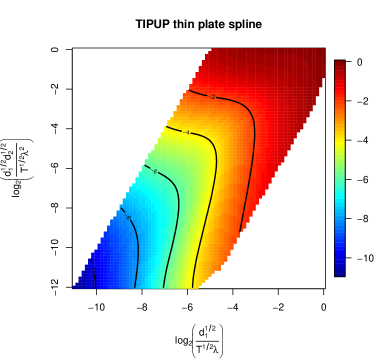
Figure 2: Logarithm of the average loss of estimating ${\mbox{\boldmath$u$}}_{1}$ using the TIPUP vs the logarithms of the two components in the convergence rate equation (67)

The figures clearly confirm the theoretical results. Note that, when the two terms in (67) are of different rates (off 45 degree line in the figure), one of the rates would dominate hence the contour lines of the error rate should be either horizontal or vertical in the figure as $(x,y)$ moves away from the 45 degree line. For negative AR coefficient $\phi=-0.6$ in the factor dynamics, the results are similar.

We also considered a parametric fit of the TIPUP error rate. Specifically, we fit the following model to the average loss $L$ of estimating ${\mbox{\boldmath$u$}}_{1}$:

$$\log_{2}(L)\sim\log_{2}(c_{1}2^{\nu_{1}}+c_{6}2^{\nu_{2}}),$$ (68)

where

$$\nu_{1} = c_{2}\log_{2}d_{1}+c_{3}\log_{2}d_{2}+c_{4}\log_{2}\lambda+c_{5}\log_{2}T$$

$$\nu_{2} = c_{7}\log_{2}d_{1}+c_{8}\log_{2}d_{2}+c_{9}\log_{2}\lambda+c_{10}\log_{2}T.$$

and compared the empirical fit with the theoretical results in Theorem 2. The results are shown in Table 1. They are reasonably close.

	$c_{1}$	$c_{2}$	$c_{3}$	$c_{5}$	$c_{5}$	$c_{6}$	$c_{7}$	$c_{8}$	$c_{9}$	$c_{10}$
Thm 2		0.50	0.00	-1.00	-0.50		0.50	0.50	-2.00	-0.50
fitted	1.19	0.51	-0.06	-0.73	-0.65	0.36	0.72	0.58	-1.92	-0.45

Table 1: Comparison between the theoretical rates and the simulated rates for the TIPUP procedure.

For TOPUP, the convergence rate based on Theorem 1 and (48) in this case is

$$\frac{(d_{1}d_{2})^{1/2}}{T^{1/2}\lambda}+\frac{(d_{1}d_{2}^{2})^{1/2}}{T^{1/2}\lambda^{2}}.$$ (69)

Similarly, let $x=log_{2}\left(\frac{(d_{1}d_{2})^{1/2}}{T^{1/2}\lambda}\right)$ and $y=log_{2}\left(\frac{(d_{1}d_{2}^{2})^{1/2}}{T^{1/2}\lambda^{2}}\right)$ and $z$ be the logarithm of the average of corresponding estimation error over 100 runs. Figure 3 shows the results. The picture is not as clean as that of the TIPUP estimator, but it shows the trend.

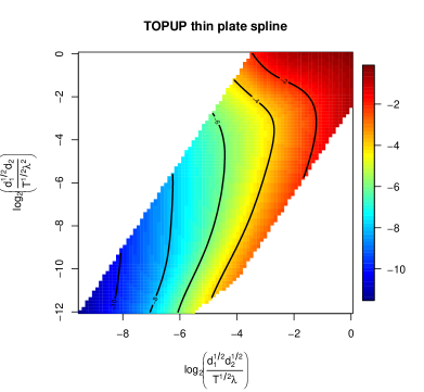
Figure 3: Logarithm of the average loss of estimating ${\mbox{\boldmath$u$}}_{1}$ using the TOPUP vs the logarithms of the two components in the convergence rate equation (69)

Again, we fit the estimation error using (68) and compared it with the theoretical result in (69), shown in Table 2. There is some discrepancy though, possibly due to the limited range of the simulation setting. The results for multiple rank cases and three dimensional tensor time series show similar patterns.

	$c_{1}$	$c_{2}$	$c_{3}$	$c_{5}$	$c_{5}$	$c_{6}$	$c_{7}$	$c_{8}$	$c_{9}$	$c_{10}$
Thm 1		0.50	0.50	-1.00	-0.50		0.50	1.00	-2.00	-0.50
fit	0.83	0.51	-0.16	-0.66	-0.55	0.36	1.21	1.03	-2.51	-0.70

Table 2: Comparison between the theoretical rates and the simulated rates for the TOPUP procedure.

To compare the performance of different methods in finite samples, we generated observations from the following two dimensional model

$${\mbox{\boldmath$X$}}_{t}=2{\mbox{\boldmath$A$}}_{1}{\mbox{\boldmath$F$}}_{t}{\mbox{\boldmath$A$}}_{2}^{\top}+{\mbox{\boldmath$E$}}_{t}$$

where ${\mbox{\boldmath$F$}}_{t}=[f_{1t},f_{2t}]$ is a $1\times 2$ factor, with two independent AR(1) processes $f_{it}=\phi_{i}f_{it-1}+e_{it}$. The noise ${\mbox{\boldmath$E$}}_{t}$ is generated the same way as the simulation in the rank one case. The elements of the loadings ${\mbox{\boldmath$A$}}_{1}$ (a $d_{1}\times 1$ matrix) and ${\mbox{\boldmath$A$}}_{2}$ (a $d_{2}\times 2$ matrix) are generated from i.i.d N(0,1), then normalized so that $||{\mbox{\boldmath$A$}}_{1}||=1$ (${\mbox{\boldmath$A$}}_{1}$ is vector) and ${\mbox{\boldmath$A$}}_{2}$ is orthonormal through QR decomposition. We use dimension $d_{1}=d_{2}=16$ here. Figures 4 and 5 show the comparison of the estimation methods, using boxplots of the logarithm of the estimation error in 100 simulation runs. The estimation error of ${\mbox{\boldmath$A$}}_{1}$ is calculated the same way as that in the rank one case (since ${\mbox{\boldmath$A$}}_{1}$ is a vector). The estimation error of ${\mbox{\boldmath$A$}}_{2}$ is the spectral norm of the difference between $\hat{{\mbox{\boldmath$A$}}}_{2}(\hat{{\mbox{\boldmath$A$}}}_{2}^{\top}\hat{{\mbox{\boldmath$A$}}}_{2})^{-1}\hat{{\mbox{\boldmath$A$}}}_{2}^{\top}$ and ${\mbox{\boldmath$A$}}_{2}({\mbox{\boldmath$A$}}_{2}^{\top}{\mbox{\boldmath$A$}}_{2})^{-1}{\mbox{\boldmath$A$}}_{2}^{\top}$, i.e., the difference of the two projection matrices. TOPUP1 and TOPUP2 denote the results using the TOPUP method with $h_{0}=1$ and $h_{0}=2$, respectively. Similarly, TIPUP1 and TIPUP2 denote the results using the TIPUP method with $h_{0}=1$ and $h_{0}=2$, respectively. UP denotes the results using simple tensor decomposition. The left panel is for estimating ${\mbox{\boldmath$A$}}_{1}$ and the right panel for ${\mbox{\boldmath$A$}}_{2}$.

Figure 4 shows the results of using $\phi_{1}=0.8$ and $\phi_{2}=-0.8$ in the AR processes of the factors and sample sizes $T=256$ and $1024$. Note that with $\phi_{1}=0.8$ and $\phi_{2}=-0.8$, we have

$$\mathbb{E}[{\mbox{\boldmath$F$}}_{t}{\mbox{\boldmath$F$}}_{t-1}^{\top}]=(\phi_{1}+\phi_{2})\sigma_{f}^{2}=0.$$

It violates the condition for the TIPUP in estimating ${\mbox{\boldmath$A$}}_{1}$. Essentially the signal in $\sum_{t=h+1}^{T}{\mbox{\boldmath$X$}}_{t}{\mbox{\boldmath$X$}}_{t-h}^{\top}$, ($h=1$), completely cancelled out in the TIPUP procedure in estimating ${\mbox{\boldmath$A$}}_{1}$ when $h_{0}=1$. Hence the results of TIPUP1 in the two left panels in Figure 4 are significantly worse than the respective TOPUP1. On the other hand, the cancellation does not happen fully with $h_{0}=2$, because in this case, $\mathbb{E}[{\mbox{\boldmath$F$}}_{t}{\mbox{\boldmath$F$}}_{t-2}^{\top}]=(\phi_{1}^{2}+\phi_{2}^{2})\sigma_{f}^{2}>0$ for the $h=2$ term. Hence TIPUP2 is comparable to that of TOPUP2 and TOPUP1. However, notice that when the sample size $T$ is larger, TIPUP2 is slightly worse that TOPUP2 and TOPUP1, due to the fact that the cancellation makes the signal weaker, and lag 2 autocorrelation is also weaker than lag 1. The TOPUP does not have such a cancellation problem since it is based on the sum of the squares of column-wise autocovariance. Note that the cancellation problem should not be very common in practice. For example, there is no cancellation for estimating ${\mbox{\boldmath$A$}}_{2}$ when using the TIPUP in this setting, since $\mathbb{E}[{\mbox{\boldmath$F$}}_{t}^{\top}{\mbox{\boldmath$F$}}_{t-1}]$ is a full rank matrix. And since the TIPUP in general has a faster convergence rate, its performance is better than that of the TOPUP, especially for small sample sizes, as shown in the right panel of Figure 4.

Figure 5 shows the results of using $\phi_{1}=0.8$ and $\phi_{2}=-0.7$ in the AR processes of the factors. Here although $\mathbb{E}[{\mbox{\boldmath$F$}}_{t}{\mbox{\boldmath$F$}}_{t-1}^{\top}]$ is not zero, TIPUP1 with $h_{0}=1$ for estimating ${\mbox{\boldmath$A$}}_{1}$ is still worse than TOPUP due to the partial cancellation, though not as severe as that in the complete cancellation $\phi_{2}=-0.8$ case.

Figure 4: Finite sample comparison between TIPUP, TOPUP and UP with different $h_{0}$. $\phi_{1}=0.8$, $\phi_{2}=-0.8$

Figure 5: Finite sample comparison between TIPUP, TOPUP and UP with different $h_{0}$. $\phi_{1}=0.8$, $\phi_{2}=-0.7$

The UP procedure is always the worst, due to the contemporary correlation in ${\mbox{\boldmath$E$}}_{t}$. Simulations using other settings show similar results.

7 Applications

7.1 Tensor factor models for import-export transport networks

Here we analyze the multi-category import-export network data as illustrated in Figure 1. The dataset contains the monthly total export among 22 countries in North American and Europe in 15 product categories from January 2010 to December 2016 (length 84), so that the original dataset can be viewed as a 4 way tensor of dimension $22\times 22\times 15\times 84$, with missing value for the total export from any country to itself. For simpliciy, we treated the missing diagonal values as zero in the analysis. More sophisticated imputation can be implemented. The details of the data, countries and product categories are given in Appendix B. Following Linnemann, (1966), to reduce the effect of incidental transactions of large trades or unusual shipping delays, a three-month moving average of the series is used, so that ${\cal X}_{t}\in\mathbb{R}^{22\times 23\times 15}$ with $t=1,\ldots,82$. Each element $x_{i,j,k,t}$ is the three month moving average of total export from country $i$ to country $j$ in category $k$ in the $t$-th month.

Figure 6 shows the total volume from year 2010 to 2017 in two categories of products (Machinery and Electronic, and Footwear and Headwear) among 22 countries in North American and Europe. The arrows show the trade direction and the width of an arrow reflects the volume of the trade. Clearly the networks are quite different for different product categories. For example, Mexico is a large importer and exporter of Machinery and Electronic as it serves as one of the major part suppliers in the product chain of machinery and electronics. On the other hand, Italy is the largest exporter of Footwear and Headwear.

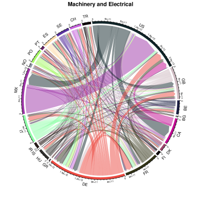
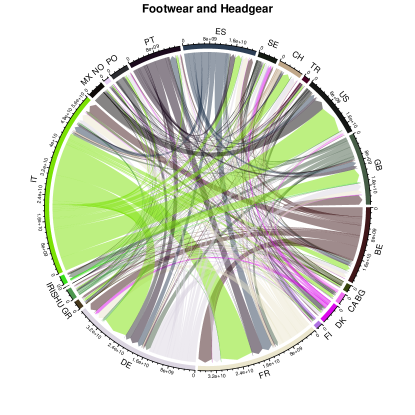
Figure 6: Time aggregated import-export volume of Machinery and Electronic products and Footwear and Headwear products among 22 countries in North American and Europe.

Under our general framework presented in Section 3, we use the following model for the dynamic transport networks. Let ${\cal X}_{t}$ be the observed tensor at time $t$. The element $x_{i_{1}i_{2}i_{3},t}$ is the trading volume from country $i_{1}$ (the exporter) to country $i_{2}$ (the importer) of product type $i_{3}$. Let

$${\cal X}_{t}={\cal F}_{t}\times_{1}{\mbox{\boldmath$A$}}_{1}\times_{2}{\mbox{\boldmath$A$}}_{2}\times_{3}{\mbox{\boldmath$A$}}_{3}+{\cal E}_{t}$$ (70)

where ${\cal X}_{t}\in\mathbb{R}^{d_{1}\times d_{2}\times d_{3}}$ ($d_{1}=d_{2}$), ${\cal F}_{t}\in\mathbb{R}^{r_{1}\times r_{2}\times r_{3}}$ ($r\ll d$), and ${\mbox{\boldmath$A$}}_{i}\in\mathbb{R}^{d_{i}\times r_{i}}$. This is similar to the DEDICOM model (Harshman,, 1978; Kolda and Bader,, 2006; Kolda et al.,, 2005). Chen and Chen, (2019) provided some interpretations of the factors in a uni-category import-export network under the matrix factor model setting of Wang et al., (2019).

In the following we provide some interpretation of the model. Consider the loading matrix ${\mbox{\boldmath$A$}}_{3}$. It can be viewed as the loading matrix of a standard factor model

$${\mbox{\boldmath$x$}}_{i_{1}i_{2}\cdot,t}={\mbox{\boldmath$A$}}_{3}{\mbox{\boldmath$f$}}^{(3)}_{i_{1}i_{2},t}+{\mbox{\boldmath$\mathnormal{\varepsilon}$}}^{(3)}_{i_{1}i_{2}\cdot,t}$$

of the mode-3 fiber ${\mbox{\boldmath$x$}}_{i_{1}i_{2}\cdot,t}$ for all $(t,i_{1},i_{2})$. This is essentially unfolding the four dimensional $d_{1}\times d_{2}\times d_{3}\times T$ tensor ${\cal Y}$ into a $d_{3}\times(d_{1}d_{2}T)$ matrix and fit a standard factor model with $d_{1}d_{2}T$ factors, each a vector of dimension $r_{3}$. These factors drive the co-moment of all mode-3 fibers ${\cal X}_{i_{1},i_{2},\cdot,t}$ at time $t$. The loading matrix reflects how each element of the mode-3 fiber is related to the factors. Note that this scheme is only for interpretation. Th estimation procedure is based on a different set-up.

Table 3 shows an estimate of ${\mbox{\boldmath$A$}}_{3}$ of the import-export data under the tensor factor model, using $r_{3}=6$ factors. The estimation is based on the TIPUP procedure with $h_{0}=2$. The loading matrix is rotated using the varimax procedure for better interpretation. All numbers are multiplied by 30 then truncated to integers for clearer viewing.

	1	2	3	4	5	6
Animal and Animal Products	0	0	0	0	6	-1
Vegetable Products	2	1	-1	0	5	0
Foodstuffs	0	0	1	2	6	1
Mineral Products	0	30	0	0	0	0
Chemicals and Allied Industries	-1	-1	29	-1	2	-1
Plastics and Rubbers	0	0	1	0	16	-3
Raw Hides, Skins, Leather and Furs	0	0	0	0	1	0
Wood and Wood Products	-2	2	0	2	7	1
Textiles	1	-1	0	-1	6	0
Footwear and Headgear	0	0	0	0	1	0
Stone and Glass	-1	0	0	0	4	29
Metals	-1	1	0	1	19	-1
Machinery and Electrical	29	0	-1	0	3	-1
Transportation	0	0	0	30	0	0
Miscellaneous	7	3	8	3	-9	6

Table 3: Estimated loading matrix ${\mbox{\boldmath$A$}}_{3}$ for category fiber. Matrix is rotated via varimax. Elements are multiplied by 30 and truncated to integer.

It can be seen that there is a group structure. For example, Factors 1, 2, 3, 4 and 6 can be interpreted as the Machinery and Electrical factor, Mineral factor, Chemicals factor, Transportation factor and Stone and Glass factor, respectively, since the corresponding product categories load heavily and almost exclusively on them. On the other hand, Factor 5 is mixed, with large loadings by Metals and Plastics/Rubbers, and medium loadings by Animal, Vegetable and Food products. We will view each factor as a ’condensed product group’. Figure 7 shows the clustering of the product categories according to their loading vectors.

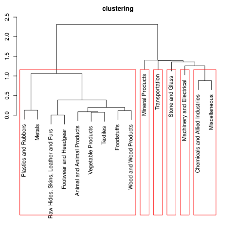
Figure 7: Clustering of product categories by their loading coefficients

The factor matrix ${\cal F}_{\cdot,\cdot,i_{3},t}$ (for a fixed $i_{3}$) can be viewed as the trading pattern among several trading hubs for the $i_{3}$-th condensed product groups (product factor). One can imagine that the export of a product by a country would first go through a virtual ’export hub’, then to a virtual ’import hub’, before arriving at the country that imports the product. Each row of the matrix ${\mbox{\boldmath$F$}}_{\cdot,\cdot,i_{3},t}$ represents an export hub and each column represents an import hub. The elements ${\cal F}_{i_{1},i_{2},i_{3},t}$ can be viewed as the volume of the condensed product group $i_{3}$ moved from export hub $i_{1}$ to import hub $i_{2}$ at time $t$. The corresponding loading matrices ${\mbox{\boldmath$A$}}_{1}$ and ${\mbox{\boldmath$A$}}_{2}$ reflects the trading activities of each country through each of the export and import hubs, respectively. We normalize each column of the loading matrices to sum up to one, so the value can be viewed as the proportion of activities of each country contributes to the hubs. Tables 4 and 5 show the estimated loading matrices ${\mbox{\boldmath$A$}}_{1}$ and ${\mbox{\boldmath$A$}}_{2}$ after varimax rotation and column normalization, using four export hubs (E1 to E4) and four import hubs (I1 to I4). All values are in percentage. There are a few negative values since we do not constrain the loadings to be positive. The interpretation of the negative values is tricky. Fortunately there are not many and the values are small. From Table 4, it is seen that Canada, US and Mexico heavily load on export hubs E1, E2 and E4, respectively, while European countries mainly load on export hub E3. The clustering based on loading coefficients of ${\mbox{\boldmath$A$}}_{1}$ of each country is shown in the left panel of Figure 8. The three countries in North America are very different from the European countries. In Europe, Germany behaves differently from the others as an exporter. For imports, seen from Table 5, US and Germany load heavily on hubs I1 and I4, respectively, while Canada and Mexico share hub I2. The European countries other than Germany mainly load on hub I3. The clustering based on loading coefficients of ${\mbox{\boldmath$A$}}_{2}$ of each country is shown in the right panel of Figure 8. It seems that the European countries (other than Germany) can be divided into two groups of similar import behavior, mainly based on the size of their economies.

	BE	BG	CA	DK	FI	FR	DE	GR	HU	IS	IR	IT	MX	NO	PO	PT	ES	SE	CH	TR	US	GB
1	4	0	80	0	1	2	-4	0	0	0	5	0	-3	3	0	1	2	0	3	0	3	5
2	-1	0	-4	0	0	1	-6	0	1	0	-2	2	1	1	1	0	0	0	1	0	102	1
3	9	0	-1	2	1	12	29	0	2	0	7	9	-3	1	4	1	7	3	6	2	1	8
4	-8	0	5	0	0	0	15	0	0	0	-7	2	104	-2	-2	-1	-4	1	-3	-1	0	2

Table 4: Estimated loading matrix ${\mbox{\boldmath$A$}}_{1}$ for the export fiber (hub). Matrix is rotated via varimax and column normalized. Values are in percentage.

	BE	BG	CA	DK	FI	FR	DE	GR	HU	IS	IR	IT	MX	NO	PO	PT	ES	SE	CH	TR	US	GB
1	1	0	2	0	0	-1	0	0	0	0	0	0	-2	0	0	0	1	0	0	0	100	-1
2	0	0	57	0	0	2	-5	0	0	0	1	-2	44	0	-1	-1	-2	-1	0	1	0	7
3	10	1	-2	3	2	22	-3	1	4	0	1	11	0	2	6	2	6	5	8	4	0	18
4	7	0	4	0	0	0	68	1	-2	0	4	4	1	1	-2	1	8	0	-2	2	0	5

Table 5: Estimated loading matrix ${\mbox{\boldmath$A$}}_{2}$ for the import fiber (hub). Matrix is rotated via varimax and column normalized. Values are in percentage.

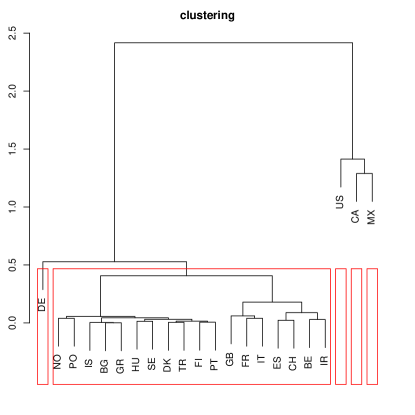
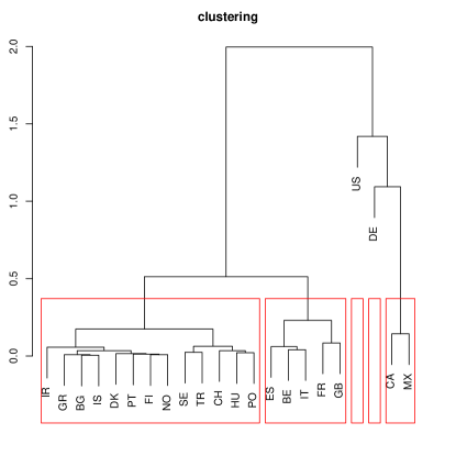
Figure 8: Clustering of countries by their export (left) and import (right) loading coefficients

The left panel of Figure 9 shows the trade transport network for the condensed product group 1 (mainly Machinery and Electrical). Several interesting features emerge. Export hub E3 (European hub) has the largest trading volume, and the goods mainly go to import hub I3 (European hub) and hub I1 (US hub). This is understandable as trades among the many countries in Europe accumulate, and US is one of the largest importers. Mexico dominates export hub E4 and it mainly exports to import hub I1, used by US, confirming what is shown in the left panel of Figure 6. US is also a large exporter of machinery and electrical, occupying export hub E2, which mainly exports to import hub I2 used by Mexico and Canada.

On the other hand, for the network of condensed product group 2 (mainly mineral products) shown in right panel of Figure 9, the dynamic is quite different. Export hub E1, mainly used by Canada, is the largest hub for mineral products. The import hub I1 is the largest import hub, mainly used by US. Most of its volume come through export hubs E1 (used mainly by Canada) and E4 (used mainly by Mexico). The network plots of other product groups are shown in Appendix B.

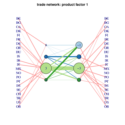
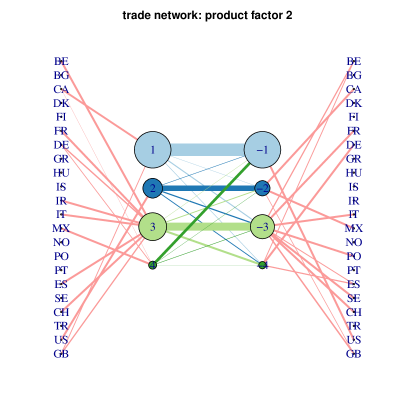
Figure 9: Trade network for condensed product group 1 (left) and group 2 (right). Export and import hubs are on the left and right of the center network respectively. Line width is proportional to the total volume of trade between the hubs for the last three years (2015 to 2017). Vertex size is proportional to total volume of trades through the hub. The line width between the countries and the hubs is proportional to the corresponding loading coefficients, for coefficients larger than 0.05 only.

Figure 10 shows the normalized trading volumes among the hubs (factors) to show the variation in trading through time. Note that the scales are very different among the figures.

Figure 10: Trading volumes among the hubs (factors) of condensed product group 1. Rows are for export and columns for import.

We remark that this analysis is just for illustration and showcasing the interpretation of the model. A more formal analysis would include the determination of the number of factors and model comparison procedures.

7.2 Taxi traffic in New York city

In this example we analyze taxi traffic pattern in New York city. The data includes all individual taxi rides operated by Yellow Taxi within New York City, maintained by the Taxi & Limousine Commission of New York City and published at

https://www1.nyc.gov/site/tlc/about/tlc-trip-record-data.page.

The dataset contains 1.4 billion trip records within the period of January 1, 2009 to December 31, 2017, among these 1.2 billion are for rides within Manhattan Island. Each trip record includes fields capturing pick-up and drop-off dates/times, pick-up and drop-off locations, trip distances, itemized fares, rate types, payment types, and driver-reported passenger counts. As we are interested in the movements of passengers using the taxi service, our study focuses on the pick-up and drop-off dates/times, and pick-up and drop-off locations of each ride. To simplify the discussion, we only consider rides within Manhattan Island.

The pick-up and drop-off location in Manhattan are coded according to 69 predefined zones in the dataset after 2016 and we will use them to classify the pick-up and drop-off locations. To account for time variation during the day, we divide each day into 24 hourly periods. The first hourly period is from 0am to 1am. The total number of rides moving among the zones within each hour is recorded, yielding a ${\cal X}_{t}\in\mathbb{R}^{69\times 69\times 24}$ tensor for each day. Here $x_{i_{1},i_{2},i_{3},t}$ is the number of trips from zone $i_{1}$ (the pick-up zone) to zone $i_{2}$ (the drop-off zone) and the pickup time within the $i_{3}$-th hourly period in day $t$. We consider business day and non-business day separately and ignore the gaps created by the separation. Hence we will analyze two tensor time series. The business-day series is 2,262 days long, and the non-business-day series is 1,025 day long, within the period of January 1, 2009 to December 31, 2017.

After some exploratory analysis, we decide to use the tensor factor model with a $4\times 4\times 4$ core factor tensor and estimate the model using the TIPUP estimator with $h_{0}=1$. The TOPUP estimator produces similar results.

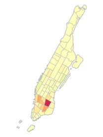
Figure 11: Loadings on four pickup factors for business day series

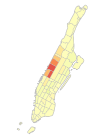
Figure 12: Loadings on four pickup factors for non-business day series

Figure 11 shows the heatmap of the loading matrix ${\mbox{\boldmath$A$}}_{1}$ (related to pick-up locations) of the 69 zones in Manhattan. It is seen that during business days, the midtown/Times square area is heavily loaded on Factor 1, upper east side on Factor 2, upper west side on Factor 3 and lower east side on Factor 4. For non-business days, the loading matrix is significantly different, as shown in Figure 12. The area on the lower west side near Chelsea (with many restaurants and bars) that heavily loads on the first factor is not active for pickups during the business day.

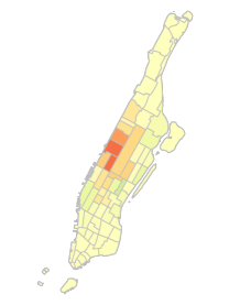
Figure 13: Loadings on four dropoff factors for business day series

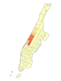
Figure 14: Loadings on four dropoff factors for non-business day series

Figures 13 and 14 show the loading matrices ${\mbox{\boldmath$A$}}_{2}$ (related to dropoff locations) for business days and non-business days, respectively. For dropoff during business days, the areas that load heavily on the factors are quite similar to that for pick-up, except the area that loads heavily on Factor 2. This area is around Union Square which is a big transportation hub servicing the surrounding tri-state area (New York, Connecticut and New Jersey), and a heavy shopping/restaurant area. For non-business days, the dropoff area that heavily loads on Factor 3 (Yorkvill/Lenox hill) is different from all the areas used for both pickup and dropoff and for both business days and non-business days. To simplify our presentation and to show comparable results in different settings, we will roughly match the pickup and dropoff factors by their corresponding heavily loaded areas, shown in Table 6 with brief area descriptions.

Area	source factor				description
	Business		non-Bus
	p	d	p	d
1 Upper east	2	1	3		affluent neighborhoods and museums
2 Midtown/Times square	1	3		1	tourism and office buildings
3 Upper west/Lincoln square	3	4	4	4	affluent neighborhoods and performing arts
4 East village/Lower east	4		2		historic district with art
5 Union square		2		2	transportation hub with shops and restaurants
6 Clinton east/Chelsea			1		lots of restaurants and bars
7 Yorkvill/Lenox hill				3	a few universities

Table 6: Label of representing areas identified under the tensor factor model with area description. “p” stands for pickup and “d” for dropoff.

Tables 7 and 8 show the loading matrix ${\mbox{\boldmath$A$}}_{3}$ (on the time of day dimension) for business day and non-business day, respectively, after varimax rotation. The shaded cells roughly show the dominating periods of each of the factors, though the change is more continuously and smooth. It is seen that, for business days, the morning rush-hours between 6am to 9am are heavy and almost exclusively loaded on factor 1 and we will name this factor the morning rush-hour factor. The business hours from 8am to 3pm heavily load on Factor 2 (the business hour factor), the evening rush-hours from 3pm to 8pm load heavily on Factor 3 (the evening rush-hour factor) and the night life hours from 8pm to 1am load on Factor 4 (the night life factor). On the other hand, for nonbusiness days, we have morning activities between 8am to 1pm (the morning factor), afternoon/evening activities between 12pm to 9pm (the afternoon/evening factor), and night activities between 9pm to 12am (the early night factor) and 12am to 4am (the late night factor).

0am		2		4		6		8		10		12pm		2		4		6		8		10		12am
1	-2	-1	-1	-1	1	10	47	72	42	14	2	-6	-11	-9	-8	-5	-1	5	5	4	1	2	0	-2
2	0	0	0	0	-1	-4	-13	-5	32	46	36	35	38	33	29	19	9	1	-2	-5	-3	-3	-1	1
3	-5	-4	-3	-2	-1	1	4	6	-15	-25	-6	4	7	9	19	31	32	43	47	39	22	14	4	-6
4	28	18	11	7	4	1	0	-8	2	14	4	-2	-3	-2	-7	-15	-13	-11	1	19	35	41	46	47

Table 7: Estimated loading matrix ${\mbox{\boldmath$A$}}_{3}$ for hour of day fiber. Business day. Matrix is rotated via varimax. Values are in percentage.

0am		2		4		6		8		10		12pm		2		4		6		8		10		12am
1	-20	-3	11	10	5	3	9	19	34	47	47	35	23	14	10	12	3	-4	-13	-16	-14	-13	-5	10
2	19	0	-13	-11	-3	0	0	-2	-3	-2	6	17	25	29	30	27	29	34	39	33	22	17	5	-17
3	-11	3	14	7	-2	-4	-4	-3	-2	2	-1	-5	-3	1	0	4	-3	-3	2	17	20	24	45	78
4	53	52	45	37	21	8	6	5	4	2	1	2	-2	-4	-4	-6	-2	0	0	-1	4	6	0	-10

Table 8: Estimated loading matrix ${\mbox{\boldmath$A$}}_{3}$ for hour of day fiber. Non-Business day. Matrix is rotated via varimax. Values are in percentage.

Figures 15 and 16 show the traffic network plots between the areas defined in Table 6 during different time factor periods. The width of the lines reflects total traffic volume between the major areas over the entire time series (the sum of the factors $f_{k_{1}k_{2}k_{3},t}$ over time $t$.) The size of the vertices reflects total number of pickups (left vertices) and dropoffs (right vertices) in the area during the time factor period.

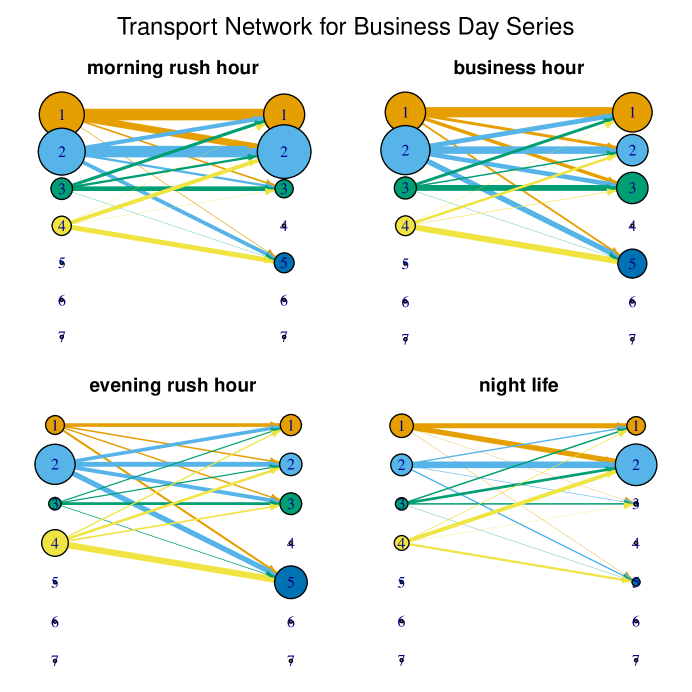
Figure 15: Network Plots during the four time factor periods for business day series

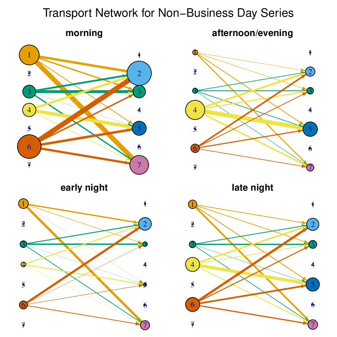
Figure 16: Network Plots during the four time factor periods for non-business day series

The figures reveal many interesting patterns. For example, during the morning rush-hours of business days, traffic mainly goes from Areas 1 and 2 (upper east and midtown) to Areas 2 (midtown). There is only a small amount of traffic to Area 5. During the business hours and early evening hours, traffic is mainly within Areas 1 and 2. During the evening rush-hour, the main pickup area is midtown and the main dropoff area is the Union square where many people take public transportation to the surrounding tri-state area. During the night life hours, main traffic is towards Area 2 (midtown), since Times square is popular among tourists and night-life goers.

For non-business days, the pattern is very different. During morning time from 8am to 12pm, most traffic takes place from Area 6 (Chelsea) to Area 2 (midtown) and from Area 1 (upper east side) to Area 7 (Yorkvill/Lenox hill); during afternoon/evening from 12pm to 9pm, many riders take taxi from Area 4 (lower east) to Area 5 (Union square); during early night (from 8pm to 12am), the traffic volume is much smaller, mainly from Areas 1 (upper east) and 6 (Chelsea) to Areas 7 (Yorkvill/Lenox hill) and 2 (midtown); during late night from 12am to 5am, the traffic is heavier than early night, mainly dominated by pickups from Areas 4 (lower east) and 6 (Chelsea) and dropoffs in Areas 5 (Union square) and 2 (midtown). The late night dropoff to Union square is very plausible since people need to go to transportation hub to go back home after a long night in New York city after midnight.

Again, this analysis is for demonstration of the tensor factor model only. More thorough and sophisticated analysis may be needed to fully understand the traffic pattern.

Appendix A: Proof of the theorems

We first prove Theorem 2 as the analysis is simpler and facilitates the proof of Theorem 1.

Proof of Theorem 2. It suffices to consider $k=1$ and $K=2$ as the TIPUP begins with mode-$k$ matrix unfolding in (17). We observe a matrix time series with ${\mbox{\boldmath$X$}}_{t}={\mbox{\boldmath$A$}}_{1}{\mbox{\boldmath$F$}}_{t}{\mbox{\boldmath$A$}}_{2}^{\top}+{\mbox{\boldmath$E$}}_{t}\in\mathbb{R}^{d_{1}\times d_{2}}$ and

$${\mbox{\boldmath$V$}}^{*}_{1,h}=\sum_{t=h+1}^{T}\frac{{\mbox{\boldmath$X$}}_{t-h}{\mbox{\boldmath$X$}}_{t}^{\top}}{T-h}\in\mathbb{R}^{d_{1}\times d_{1}},\quad{\mbox{\boldmath$\mathnormal{\Theta}$}}^{*}_{1,h}=\sum_{t=h+1}^{T}\frac{{\mbox{\boldmath$A$}}_{1}{\mbox{\boldmath$F$}}_{t-h}{\mbox{\boldmath$A$}}_{2}^{\top}{\mbox{\boldmath$A$}}_{2}{\mbox{\boldmath$F$}}_{t}^{\top}{\mbox{\boldmath$A$}}_{1}^{\top}}{T-h}\in\mathbb{R}^{d_{1}\times d_{1}}.$$

Let ${\mbox{\boldmath$\mathnormal{\Delta}$}}^{*}_{1}$, ${\mbox{\boldmath$\mathnormal{\Delta}$}}^{*}_{2}$ and ${\mbox{\boldmath$\mathnormal{\Delta}$}}^{*}_{3}$ be respectively the three terms on the right-hand side below:

$${\mbox{\boldmath$V$}}^{*}_{1,h}-{\mbox{\boldmath$\mathnormal{\Theta}$}}^{*}_{1,h}=\sum_{t=h+1}^{T}\frac{{\mbox{\boldmath$A$}}_{1}{\mbox{\boldmath$F$}}_{t-h}{\mbox{\boldmath$A$}}_{2}^{\top}{\mbox{\boldmath$E$}}_{t}^{\top}}{T-h}+\sum_{t=h+1}^{T}\frac{{\mbox{\boldmath$E$}}_{t-h}{\mbox{\boldmath$A$}}_{2}{\mbox{\boldmath$F$}}_{t}^{\top}{\mbox{\boldmath$A$}}_{1}^{\top}}{T-h}+\sum_{t=h+1}^{T}\frac{{\mbox{\boldmath$E$}}_{t-h}{\mbox{\boldmath$E$}}_{t}^{\top}}{T-h}.$$ (71)

Let $\sigma_{*}=\sigma\big{\|}{\mbox{\boldmath$\mathnormal{\Theta}$}}^{*}_{1,0}\big{\|}_{\rm S}^{1/2}$ with the norm in (32). By Condition A, for any $u$ and $v$ in $\mathbb{R}^{d_{1}}$ we have

$$\overline{\mathbb{E}}\bigg{\{}{\mbox{\boldmath$u$}}^{\top}\bigg{(}\sum_{t=h+1}^{T}\frac{{\mbox{\boldmath$A$}}_{1}{\mbox{\boldmath$F$}}_{t-h}{\mbox{\boldmath$A$}}_{2}^{\top}{\mbox{\boldmath$E$}}_{t}^{\top}}{T^{1/2}}\bigg{)}{\mbox{\boldmath$v$}}\bigg{\}}^{2}\leq\frac{\sigma^{2}\|{\mbox{\boldmath$v$}}\|_{2}^{2}}{T}\big{\|}\sum_{t=h+1}^{T}{\mbox{\boldmath$A$}}_{2}{\mbox{\boldmath$F$}}_{t}^{\top}{\mbox{\boldmath$A$}}_{1}^{\top}{\mbox{\boldmath$u$}}\big{\|}_{2}^{2}\leq\sigma^{2}\big{\|}{\mbox{\boldmath$\mathnormal{\Theta}$}}^{*}_{1,0}\big{\|}_{\rm S}\|{\mbox{\boldmath$u$}}\|_{2}^{2}\|{\mbox{\boldmath$v$}}\|_{2}^{2}.$$

Thus for vectors ${\mbox{\boldmath$u$}}_{i}$ and ${\mbox{\boldmath$v$}}_{i}$ with $\|{\mbox{\boldmath$u$}}_{i}\|_{2}=\|{\mbox{\boldmath$v$}}_{i}\|_{2}=1$,

$$\{(T-h)^{2}/(T\sigma_{*}^{2})\}\overline{\mathbb{E}}\big{(}{\mbox{\boldmath$u$}}_{1}^{\top}{\mbox{\boldmath$\mathnormal{\Delta}$}}^{*}_{1}{\mbox{\boldmath$v$}}_{1}-{\mbox{\boldmath$u$}}_{2}^{\top}{\mbox{\boldmath$\mathnormal{\Delta}$}}^{*}_{1}{\mbox{\boldmath$v$}}_{2}\big{)}^{2}$$

$$\leq \Big{(}\|{\mbox{\boldmath$u$}}_{1}-{\mbox{\boldmath$u$}}_{2}\|_{2}\|{\mbox{\boldmath$v$}}_{1}\|_{2}+\|{\mbox{\boldmath$u$}}_{2}\|_{2}\|{\mbox{\boldmath$v$}}_{1}-{\mbox{\boldmath$v$}}_{2}\|_{2}\Big{)}^{2}$$

$$\leq 2\Big{(}\|{\mbox{\boldmath$u$}}_{1}-{\mbox{\boldmath$u$}}_{2}\|_{2}^{2}+\|{\mbox{\boldmath$v$}}_{1}-{\mbox{\boldmath$v$}}_{2}\|_{2}^{2}\Big{)}$$

$$= 2\ \mathbb{E}\big{\{}({\mbox{\boldmath$u$}}_{1}-{\mbox{\boldmath$u$}}_{2})^{\top}{\mbox{\boldmath$\mathnormal{\xi}$}}+({\mbox{\boldmath$v$}}_{1}-{\mbox{\boldmath$v$}}_{2})^{\top}{\mbox{\boldmath$\mathnormal{\zeta}$}}\big{\}}^{2}$$

where $\mathnormal{\xi}$ and $\mathnormal{\zeta}$ are iid $N(0,{\mbox{\boldmath$I$}}_{d_{1}})$ vectors. As ${\mbox{\boldmath$\mathnormal{\Delta}$}}^{*}_{1}$ is a $d_{1}\times d_{1}$ Gaussian matrix under $\overline{\mathbb{E}}$, the Sudakov-Fernique inequality yields

$$\Big{(}\frac{T-h}{T^{1/2}\sigma_{*}}\Big{)}\overline{\mathbb{E}}\big{\|}{\mbox{\boldmath$\mathnormal{\Delta}$}}^{*}_{1}\big{\|}_{\rm S}\leq\sqrt{2}\mathbb{E}\sup_{\|{\mbox{\boldmath$u$}}\|_{2}=\|{\mbox{\boldmath$v$}}\|_{2}=1}\Big{|}{\mbox{\boldmath$u$}}^{\top}{\mbox{\boldmath$\mathnormal{\xi}$}}+{\mbox{\boldmath$v$}}^{\top}{\mbox{\boldmath$\mathnormal{\zeta}$}}\big{|}=\sqrt{2}\mathbb{E}\Big{(}\|{\mbox{\boldmath$\mathnormal{\xi}$}}\|_{2}+\|{\mbox{\boldmath$\mathnormal{\zeta}$}}\|_{2}\Big{)}.$$

As $\mathbb{E}\|{\mbox{\boldmath$\mathnormal{\xi}$}}\|_{2}=\mathbb{E}\|{\mbox{\boldmath$\mathnormal{\zeta}$}}\|_{2}\leq\sqrt{d_{1}}$, it follows that for the first term on the right-hand side of (71)

$$\overline{\mathbb{E}}\big{\|}{\mbox{\boldmath$\mathnormal{\Delta}$}}^{*}_{1}\big{\|}_{\rm S}\leq\frac{\sigma_{*}(8Td_{1})^{1/2}}{T-h}=\frac{\sigma(8Td_{1})^{1/2}}{T-h}\big{\|}{\mbox{\boldmath$\mathnormal{\Theta}$}}^{*}_{1,0}\big{\|}_{\rm S}^{1/2}.$$ (72)

Similarly, $\overline{\mathbb{E}}\big{\|}{\mbox{\boldmath$\mathnormal{\Delta}$}}^{*}_{2}\big{\|}_{\rm S}\leq\sigma(8Td_{1})^{1/2}(T-h)^{-1}\big{\|}{\mbox{\boldmath$\mathnormal{\Theta}$}}^{*}_{1,0}\big{\|}_{\rm S}^{1/2}$ for the second term.

Let $h\leq T/4$. For the third term ${\mbox{\boldmath$\mathnormal{\Delta}$}}^{*}_{3}$ on the right-hand side of (71), we split the sum into two terms over the index sets, $S_{1}=\{(h,2h]\cup(3h,4h]\cup\ldots\}\cap(h,T]$ and its complement $S_{2}$ in $(h,T]$, so that $({\mbox{\boldmath$E$}}_{t-h},t\in S_{a})$ and $({\mbox{\boldmath$E$}}_{t},t\in S_{a})$ are two independent $d_{1}\times n_{a}$ centered Gaussian matrices for each $a=1,2$, with $n_{1}+n_{2}=(T-h)d_{2}$. Thus, by Lemma 1 (i),

$$\frac{\overline{\mathbb{E}}\big{\|}{\mbox{\boldmath$\mathnormal{\Delta}$}}^{*}_{3}\big{\|}_{\rm S}}{\sigma^{2}}\leq\sum_{a=1}^{2}\overline{\mathbb{E}}\bigg{\|}\sum_{t\in S_{a}}\frac{{\mbox{\boldmath$E$}}_{t-h}{\mbox{\boldmath$E$}}_{t}^{\top}}{\sigma^{2}(T-h)}\bigg{\|}_{\rm S}\leq\sum_{a=1}^{2}\frac{2\sqrt{d_{1}n_{a}}+d_{1}}{T-h}\leq\frac{\sqrt{8d_{1}d_{2}}}{\sqrt{T-h}}+\frac{2d_{1}}{T-h}.$$ (73)

We obtain the first inequality in (57) by applying (72) and (73) to (71), and the second by Cauchy-Schwarz, ${\|({\mbox{\boldmath$\mathnormal{\Delta}$}}_{1},\ldots,{\mbox{\boldmath$\mathnormal{\Delta}$}}_{h_{0}})\|_{\rm S}^{2}}\leq h_{0}\sum_{h=1}^{h_{0}}\|{\mbox{\boldmath$\mathnormal{\Delta}$}}_{h}\|_{\rm S}^{2}$. Finally, by Wedin (1972),

$$\overline{\mathbb{E}}\Big{\|}\widehat{{\mbox{\boldmath$P$}}_{1,r_{1}}}-{\mbox{\boldmath$P$}}_{1}\Big{\|}_{\rm S} \leq \frac{2}{\big{(}{\lambda}^{*}_{1}\big{)}^{2}}\bigg{\{}\frac{2\sigma(8Td_{1})^{1/2}}{T-h_{0}}\big{\|}{\mbox{\boldmath$\mathnormal{\Theta}$}}^{*}_{1,0}\big{\|}_{\rm S}^{1/2}+\frac{\sigma^{2}\sqrt{8d_{1}d_{2}}}{\sqrt{T-h_{0}}}+\frac{2\sigma^{2}d_{1}}{T-h_{0}}\bigg{\}}$$

As $\sqrt{T}\big{\|}{\mbox{\boldmath$\mathnormal{\Theta}$}}^{*}_{1,0}\big{\|}_{\rm S}^{1/2}\geq\sqrt{T-h}{\lambda}^{*}_{1}$ by (43) and $\overline{\mathbb{E}}\big{\|}\widehat{{\mbox{\boldmath$P$}}_{1,r_{1}}}-{\mbox{\boldmath$P$}}_{1}\big{\|}_{\rm S}\leq 1$, (58) holds automatically when $4\sigma\sqrt{8d_{1}}\geq{\lambda}^{*}_{1}\sqrt{T-h_{0}}$, whereas (58) follows from

$$\frac{2\sigma^{2}d_{1}}{T-h_{0}}\leq\frac{{\lambda}^{*}_{1}\sigma\sqrt{d_{1}}}{2\sqrt{8(T-h_{0})}}\leq\frac{\sigma\sqrt{8Td_{1}}}{16(T-h_{0})}\big{\|}{\mbox{\boldmath$\mathnormal{\Theta}$}}^{*}_{1,0}\big{\|}_{\rm S}^{1/2}$$

otherwise. Thus, (58) holds either ways. $\hfill\square$

Lemma 1.

(i) Let $G\in\mathbb{R}^{d_{1}\times n}$ and $H\in\mathbb{R}^{d_{2}\times n}$ be two centered independent Gaussian matrices such that $\mathbb{E}(u^{\top}\text{vec}(G))^{2}\leq\sigma^{2}\ \forall\ u\in\mathbb{R}^{d_{1}n}$ and $\mathbb{E}(v^{\top}\text{vec}(H))^{2}\leq\sigma^{2}\ \forall\ v\in\mathbb{R}^{d_{2}n}$. Then,

$$\mathbb{E}\big{[}\|GH^{\top}\|_{\rm S}\big{]}\leq\sigma^{2}\big{(}\sqrt{d_{1}d_{2}}+\sqrt{d_{1}n}+\sqrt{d_{2}n}\big{)}.$$

(ii) Let $G_{i}\in\mathbb{R}^{d_{1}\times d_{2}},H_{i}\in\mathbb{R}^{d_{3}\times d_{4}},i=1,\ldots,n$, be independent centered Gaussian matrices such that $\mathbb{E}(u^{\top}\text{vec}(G_{i}))^{2}\leq\sigma^{2}\ \forall\ u\in\mathbb{R}^{d_{1}d_{2}}$ and $\mathbb{E}(v^{\top}\text{vec}(H_{i}))^{2}\leq\sigma^{2}\ \forall\ v\in\mathbb{R}^{d_{3}d_{4}}$. Then,

$$\mathbb{E}\bigg{[}\bigg{\|}\hbox{\rm mat}_{1}\bigg{(}\sum_{i=1}^{n}G_{i}\otimes H_{i}\bigg{)}\bigg{\|}_{\rm S}\bigg{]}\leq\sigma^{2}\big{(}\sqrt{d_{1}n}+\sqrt{d_{1}d_{3}d_{4}}+\sqrt{nd_{2}d_{3}d_{4}}\big{)}.$$

Proof. Assume $\sigma=1$ without loss of generality.
(i) Independent of $G$ and $H$, let $\xi_{j}\in\mathbb{R}^{d_{j}}$ and $\zeta_{j}\in\mathbb{R}^{n}$, $j=1,2$, be independent standard Gaussian vectors. For $\|v_{1}\|_{2}=\|v_{2}\|_{2}=1$ and $\|w_{1}\|_{2}\vee\|w_{2}\|_{2}\leq 1$, $\mathbb{E}(v_{1}^{\top}Hw_{1}-v_{2}^{\top}Hw_{2})^{2}\leq\mathbb{E}((v_{1}-v_{2})^{\top}\xi_{2}+(w_{1}-w_{2})^{\top}\zeta_{2})^{2}$. Thus, by the Sudakov-Fernique inequality

$$\mathbb{E}\Big{[}\|GH^{\top}\|_{\rm S}\Big{|}G\Big{]} \leq \|G\|_{\rm S}\mathbb{E}\Big{[}\max_{\|u\|_{2}=\|v\|_{2}=1}(\|G\|_{\rm S}^{-1}u^{\top}G)H^{\top}v\Big{|}G\Big{]}$$

$$\leq \|G\|_{\rm S}\mathbb{E}\Big{[}\max_{\|u\|_{2}=\|v\|_{2}=1}(\|G\|_{\rm S}^{-1}u^{\top}G\zeta_{2}+\xi_{2}^{\top}v)\Big{|}G\Big{]}$$

$$= \mathbb{E}\Big{[}\max_{\|u\|_{2}=1}u^{\top}G\zeta_{2}\Big{|}G\Big{]}+\|G\|_{\rm S}\sqrt{d_{2}}.$$

Applying the same argument to $G$, we have

$$\mathbb{E}\Big{[}\|GH^{\top}\|_{\rm S}\Big{|}G\Big{]} \leq \mathbb{E}\Big{[}\max_{\|u\|_{2}=1}u^{\top}G\zeta_{2}+\|G\|_{\rm S}\sqrt{d_{2}}\Big{]}$$

$$\leq \mathbb{E}\Big{[}\|\zeta_{2}\|_{2}\max_{\|u\|_{2}=1}(u^{\top}\xi_{1}+\zeta_{1}^{\top}\zeta_{2}/\|\zeta_{2}\|_{2})+(\sqrt{d_{1}}+\sqrt{n})\sqrt{d_{2}}\Big{]}$$

$$\leq \sqrt{d_{1}n}+(\sqrt{d_{1}}+\sqrt{n})\sqrt{d_{2}}.$$

(ii) We treat $(G_{1},\ldots,G_{n})\in\mathbb{R}^{d_{1}\times d_{2}\times n}$ and $(H_{1},\ldots,H_{n})\in\mathbb{R}^{d_{3}\times d_{4}\times n}$ as tensors. Let $\xi_{i}\in\mathbb{R}^{d_{2}}$ be additional independent standard Gaussian vectors. For $u\in\mathbb{R}^{d_{1}}$ and $V\in\mathbb{R}^{d_{2}\times(d_{3}d_{4})}$,

$$\mathbb{E}\bigg{[}\bigg{\|}\hbox{\rm mat}_{1}\bigg{(}\sum_{i=1}^{n}G_{i}\otimes H_{i}\bigg{)}\bigg{\|}_{\rm S}\bigg{]}$$

$$= \mathbb{E}\bigg{[}\sup_{\|u\|_{2}=1,\|V\|_{F}=1}u^{\top}\hbox{\rm mat}_{1}(G_{1},\ldots,G_{n})\mathrm{vec}\big{(}\hbox{\rm mat}_{3}(H_{1},\ldots,H_{n})V^{\top}\big{)}\bigg{]}$$

$$\leq \sqrt{d_{1}}\mathbb{E}\bigg{[}\sup_{\|V\|_{F}=1}\|\hbox{\rm mat}_{3}(H_{1},\ldots,H_{n})V^{\top}\|_{\rm F}\bigg{]}$$

$$+\mathbb{E}\bigg{[}\sup_{\|V\|_{F}=1}(\mathrm{vec}(\xi_{1},\ldots,\xi_{n}))^{\top}\mathrm{vec}\big{(}\hbox{\rm mat}_{3}(H_{1},\ldots,H_{n})V^{\top}\big{)}\bigg{]}$$

$$= \sqrt{d_{1}}\mathbb{E}\bigg{[}\|\hbox{\rm mat}_{3}(H_{1},\ldots,H_{n})\|_{\rm S}\bigg{]}+\mathbb{E}\bigg{[}\bigg{(}\sum_{j=1}^{d_{2}}\sum_{k=1}^{d_{3}d_{4}}\bigg{(}\sum_{i=1}^{n}\xi_{i,j}\mathrm{vec}(H_{i})_{k}\bigg{)}^{2}\bigg{)}^{1/2}\bigg{]}$$

$$\leq \sqrt{d_{1}}\big{(}\sqrt{n}+\sqrt{d_{3}d_{4}}\big{)}+\sqrt{nd_{2}d_{3}d_{4}}.$$

Again, we apply the Sudakov-Fernique inequality twice above. $\hfill\square$

Proof of Theorem 1. It suffices to consider $k=1$ and $K=2$ as the TOPUP begins with mode-$k$ matrix unfolding in (8). In this case, ${\mbox{\boldmath$X$}}_{t}={\mbox{\boldmath$M$}}_{t}+{\mbox{\boldmath$E$}}_{t}\in\mathbb{R}^{d_{1}\times d_{2}}$ with ${\mbox{\boldmath$M$}}_{t}={\mbox{\boldmath$A$}}_{1}{\mbox{\boldmath$F$}}_{t}{\mbox{\boldmath$A$}}_{2}^{\top}$,

$${\mbox{\boldmath$V$}}_{1,h}=\sum_{t=h+1}^{T}\frac{{\mbox{\boldmath$X$}}_{t-h}\otimes{\mbox{\boldmath$X$}}_{t}}{T-h},\quad{\mbox{\boldmath$\mathnormal{\Theta}$}}_{1,h}=\sum_{t=h+1}^{T}\frac{{\mbox{\boldmath$M$}}_{t-h}\otimes{\mbox{\boldmath$M$}}_{t}}{T-h}.$$

Let ${\mbox{\boldmath$\mathnormal{\Delta}$}}_{1}$, ${\mbox{\boldmath$\mathnormal{\Delta}$}}_{2}$ and ${\mbox{\boldmath$\mathnormal{\Delta}$}}_{3}$ be respectively the three terms on the right-hand side below:

$$\hbox{\rm mat}_{1}\big{(}{\mbox{\boldmath$V$}}_{1,h}\big{)}-\hbox{\rm mat}_{1}\big{(}{\mbox{\boldmath$\mathnormal{\Theta}$}}_{1,h}\big{)}$$ (74)

$$= \sum_{t=h+1}^{T}\frac{\hbox{\rm mat}_{1}({\mbox{\boldmath$M$}}_{t-h}\otimes{\mbox{\boldmath$E$}}_{t})}{T-h}+\sum_{t=h+1}^{T}\frac{\hbox{\rm mat}_{1}({\mbox{\boldmath$E$}}_{t-h}\otimes{\mbox{\boldmath$M$}}_{t})}{T-h}+\sum_{t=h+1}^{T}\frac{\hbox{\rm mat}_{1}({\mbox{\boldmath$E$}}_{t-h}\otimes{\mbox{\boldmath$E$}}_{t})}{T-h}.$$

For the first term ${\mbox{\boldmath$\mathnormal{\Delta}$}}_{1}$, we notice that ${\mbox{\boldmath$M$}}_{t-h}={\mbox{\boldmath$M$}}_{t-h}{\mbox{\boldmath$P$}}_{2}$ for a fixed orthogonal projection of rank $r_{2}$. Let ${\mbox{\boldmath$U$}}_{2}\in\mathbb{R}^{d_{2}\times r_{2}}$ with orthonormal columns and ${\mbox{\boldmath$U$}}_{2}{\mbox{\boldmath$U$}}_{2}^{\top}={\mbox{\boldmath$P$}}_{2}$. For ${\cal V}\in\mathbb{R}^{d_{2}\times d_{1}\times d_{2}}$, $\hbox{\rm mat}_{1}({\mbox{\boldmath$M$}}_{t-h}\otimes{\mbox{\boldmath$E$}}_{t})\mathrm{vec}({\cal V})=\hbox{\rm mat}_{1}(({\mbox{\boldmath$M$}}_{t-h}{\mbox{\boldmath$U$}}_{2})\otimes{\mbox{\boldmath$E$}}_{t})\mathrm{vec}({\cal W})$ with ${\cal W}={\cal V}\times_{1}{\mbox{\boldmath$U$}}_{2}^{\top}\in\mathbb{R}^{r_{2}\times d_{1}\times d_{2}}$ satisfying $\|\mathrm{vec}({\cal W})\|_{2}=\|\mathrm{vec}({\cal V})\|_{2}$, so that $\|{\mbox{\boldmath$\mathnormal{\Delta}$}}_{1}\|_{\rm S}=\|{\overline{\mbox{\boldmath$\mathnormal{\Delta}$}}}_{1}\|_{\rm S}$ with

$${\overline{\mbox{\boldmath$\mathnormal{\Delta}$}}}_{1}=\sum_{t=h+1}^{T}\frac{\hbox{\rm mat}_{1}(({\mbox{\boldmath$M$}}_{t-h}{\mbox{\boldmath$U$}}_{2})\otimes{\mbox{\boldmath$E$}}_{t})}{T-h}.$$

By Condition A, for any ${\mbox{\boldmath$u$}}\in\mathbb{R}^{d_{1}}$ and ${\cal W}\in\mathbb{R}^{r_{2}\times d_{1}\times d_{2}}$

$$\overline{\mathbb{E}}\bigg{(}T^{-1/2}\sum_{t}{\mbox{\boldmath$u$}}^{T}\hbox{\rm mat}_{1}(({\mbox{\boldmath$M$}}_{t-h}{\mbox{\boldmath$U$}}_{2})\otimes{\mbox{\boldmath$E$}}_{t})\mathrm{vec}({\cal W})\bigg{)}^{2}$$

$$= T^{-1}\sum_{t}\overline{\mathbb{E}}\bigg{(}\sum_{i_{1},j_{1},i_{2},j_{2}}u_{i_{1}}({\mbox{\boldmath$M$}}_{t-h}{\mbox{\boldmath$U$}}_{2})_{i_{1},j_{1}}\big{(}{\mbox{\boldmath$E$}}_{t}\big{)}_{i_{2},j_{2}}w_{j_{1},i_{2},j_{2}}\bigg{)}^{2}$$

$$\leq T^{-1}\sum_{t}\sigma^{2}\sum_{i_{2},j_{2}}\bigg{(}\sum_{i_{1},j_{1}}u_{i_{1}}({\mbox{\boldmath$M$}}_{t-h}{\mbox{\boldmath$U$}}_{2})_{i_{1},j_{1}}w_{j_{1},i_{2},j_{2}}\bigg{)}^{2}$$

$$\leq \sigma^{2}T^{-1}\sum_{t}\sum_{i_{2},j_{2}}\sum_{j_{1}}\bigg{(}\sum_{i_{1}}u_{i_{1}}({\mbox{\boldmath$M$}}_{t-h}{\mbox{\boldmath$U$}}_{2})_{i_{1},j_{1}}\bigg{)}^{2}\sum_{j_{1}}w_{j_{1},i_{2},j_{2}}^{2}$$

$$= \sigma^{2}T^{-1}\sum_{t}\|{\mbox{\boldmath$M$}}_{t-h}^{\top}{\mbox{\boldmath$u$}}\|_{2}^{2}\big{\|}\mathrm{vec}({\cal W})\big{\|}_{2}^{2}.$$

$$\leq \sigma^{2}\big{\|}{\mbox{\boldmath$\mathnormal{\Theta}$}}^{*}_{1,0}\big{\|}_{\rm S}\|{\mbox{\boldmath$u$}}\|_{2}^{2}\big{\|}\mathrm{vec}({\cal W})\big{\|}_{2}^{2}.$$

As in the derivation of (72), it follows that for $\|{\mbox{\boldmath$u$}}_{i}\|_{2}=\|\mathrm{vec}({\cal W}_{i})\|_{2}=1$

$$\{(T-h)^{2}/(T\sigma_{*}^{2})\}\overline{\mathbb{E}}\big{\{}{\mbox{\boldmath$u$}}_{1}^{\top}{\overline{\mbox{\boldmath$\mathnormal{\Delta}$}}}_{1}\mathrm{vec}({\cal W}_{1})-{\mbox{\boldmath$u$}}_{2}^{\top}{\overline{\mbox{\boldmath$\mathnormal{\Delta}$}}}_{1}\mathrm{vec}({\cal W}_{2})\big{\}}^{2}$$

$$\leq 2\big{\{}\|{\mbox{\boldmath$u$}}_{1}-{\mbox{\boldmath$u$}}_{2}\|_{2}^{2}+\big{\|}\mathrm{vec}({\cal W}_{1}-{\cal W}_{2})\big{\|}_{2}^{2}\big{\}}.$$

As ${\overline{\mbox{\boldmath$\mathnormal{\Delta}$}}}_{1}$ is a Gaussian matrix under $\overline{\mathbb{E}}$, the Sudakov-Fernique inequality yields

$$\overline{\mathbb{E}}\big{\|}{\mbox{\boldmath$\mathnormal{\Delta}$}}_{1}\big{\|}_{\rm S}=\overline{\mathbb{E}}\big{\|}{\overline{\mbox{\boldmath$\mathnormal{\Delta}$}}}_{1}\big{\|}_{\rm S}\leq\frac{\sigma(2T)^{1/2}(\sqrt{d_{1}}+\sqrt{r_{2}d_{1}d_{2}})}{T-h}\big{\|}{\mbox{\boldmath$\mathnormal{\Theta}$}}^{*}_{1,0}\big{\|}_{\rm S}^{1/2}.$$ (75)

For the second term ${\mbox{\boldmath$\mathnormal{\Delta}$}}_{2}$, $\hbox{\rm mat}_{1}({\mbox{\boldmath$E$}}_{t-h}\otimes{\mbox{\boldmath$M$}}_{t})\mathrm{vec}({\cal V})=\hbox{\rm mat}_{1}({\mbox{\boldmath$E$}}_{t-h}\otimes({\mbox{\boldmath$U$}}_{1}^{\top}{\mbox{\boldmath$M$}}_{t}{\mbox{\boldmath$U$}}_{2}))\mathrm{vec}({\cal W})$ with ${\mbox{\boldmath$U$}}_{j}{\mbox{\boldmath$U$}}_{j}^{\top}={\mbox{\boldmath$P$}}_{j}$ and ${\cal W}={\cal V}\times_{2}{\mbox{\boldmath$U$}}_{1}^{\top}\times_{3}{\mbox{\boldmath$U$}}_{2}^{\top}\in\mathbb{R}^{d_{2}\times r_{1}\times r_{2}}$, so that $\|{\mbox{\boldmath$\mathnormal{\Delta}$}}_{2}\|_{\rm S}=\|{\overline{\mbox{\boldmath$\mathnormal{\Delta}$}}}_{2}\|_{\rm S}$ with

$${\overline{\mbox{\boldmath$\mathnormal{\Delta}$}}}_{2}=\sum_{t=h+1}^{T}\frac{\hbox{\rm mat}_{1}({\mbox{\boldmath$E$}}_{t-h}\otimes({\mbox{\boldmath$U$}}_{1}^{\top}{\mbox{\boldmath$M$}}_{t}{\mbox{\boldmath$U$}}_{2}))}{T-h}\in\mathbb{R}^{d_{1}\times d_{2}r_{1}r_{2}}.$$

Moreover, for ${\mbox{\boldmath$u$}}\in\mathbb{R}^{d_{1}}$ and ${\cal W}\in\mathbb{R}^{d_{2}\times r_{1}\times r_{2}}$,

$$\overline{\mathbb{E}}\bigg{(}T^{-1/2}\sum_{t}{\mbox{\boldmath$u$}}^{T}\hbox{\rm mat}_{1}({\mbox{\boldmath$E$}}_{t-h}\otimes({\mbox{\boldmath$U$}}_{1}^{\top}{\mbox{\boldmath$M$}}_{t}{\mbox{\boldmath$U$}}_{2}))\mathrm{vec}({\cal W})\bigg{)}^{2}$$

$$= T^{-1}\sum_{t}\overline{\mathbb{E}}\bigg{(}\sum_{i_{1},j_{1},i_{2},j_{2}}u_{i_{1}}({\mbox{\boldmath$E$}}_{t-h})_{i_{1}.j_{2}}({\mbox{\boldmath$U$}}_{1}^{\top}{\mbox{\boldmath$M$}}_{t}{\mbox{\boldmath$U$}}_{2})_{i_{2}.j_{2}}w_{j_{1},i_{2},j_{2}}\bigg{)}^{2}$$

$$\leq \sigma^{2}T^{-1}\sum_{t}\sum_{i_{1},j_{1}}\bigg{(}\sum_{i_{2},j_{2}}u_{i_{1}}({\mbox{\boldmath$U$}}_{1}^{\top}{\mbox{\boldmath$M$}}_{t}{\mbox{\boldmath$U$}}_{2})_{i_{2}.j_{2}}w_{j_{1},i_{2},j_{2}}\bigg{)}^{2}$$

$$= \sigma^{2}\|{\mbox{\boldmath$u$}}\|_{2}^{2}\sum_{j_{1}}T^{-1}\sum_{t}{\rm trace}\Big{(}({\mbox{\boldmath$U$}}_{1}^{\top}{\mbox{\boldmath$M$}}_{t}{\mbox{\boldmath$U$}}_{2}){\cal W}^{(2,3)}_{j_{1}}\Big{)}^{2}$$

$$\leq \sigma^{2}\|{\mbox{\boldmath$u$}}\|_{2}^{2}\sum_{j_{1}}\big{\|}{\mbox{\boldmath$\mathnormal{\Theta}$}}_{1,0}\big{\|}_{\rm op}\big{\|}{\cal W}^{(2,3)}_{j_{1}}\big{\|}_{\rm F}^{2}$$

$$= \sigma^{2}\big{\|}{\mbox{\boldmath$\mathnormal{\Theta}$}}_{1,0}\big{\|}_{\rm op}\|{\mbox{\boldmath$u$}}\|_{2}^{2}\big{\|}\mathrm{vec}({\cal W})\big{\|}_{2}^{2}.$$

Thus, as ${\cal W}$ is of dimension $d_{2}\times r_{1}\times r_{2}$, the derivation of (75) yields

$$\overline{\mathbb{E}}\big{\|}{\mbox{\boldmath$\mathnormal{\Delta}$}}_{2}\big{\|}_{\rm S}=\overline{\mathbb{E}}\big{\|}{\overline{\mbox{\boldmath$\mathnormal{\Delta}$}}}_{2}\big{\|}_{\rm S}\leq\frac{\sigma(2T)^{1/2}(\sqrt{d_{1}}+\sqrt{d_{2}r_{1}r_{2}})}{T-h}\big{\|}{\mbox{\boldmath$\mathnormal{\Theta}$}}_{1,0}\big{\|}_{\rm op}^{1/2}.$$ (76)

For the third term ${\mbox{\boldmath$\mathnormal{\Delta}$}}_{3}$, we partition $(h,T]$ as $S_{1}\cup S_{2}$ as in the derivation of (73), so that by Lemma 1 (ii)

$$\overline{\mathbb{E}}\big{\|}{\mbox{\boldmath$\mathnormal{\Delta}$}}_{3}\big{\|}_{\rm S} \leq \sum_{a=1}^{2}\mathbb{E}\bigg{\|}\hbox{\rm mat}_{1}\bigg{(}\sum_{t\in S_{a}}\frac{{\mbox{\boldmath$E$}}_{t-h}\otimes{\mbox{\boldmath$E$}}_{t}}{T-h}\bigg{)}\bigg{\|}_{\rm S}$$ (77)

$$\leq \sum_{a=1}^{2}\frac{\sigma^{2}\big{(}\sqrt{d_{1}|S_{a}|}+d_{1}\sqrt{d_{2}}+d_{2}\sqrt{|S_{a}|d_{1}}\big{)}}{T-h}$$ (78)

$$\leq \frac{\sigma^{2}(1+d_{2})\sqrt{2d_{1}}}{\sqrt{T-h}}+\frac{2\sigma^{2}d_{1}\sqrt{d_{2}}}{T-h}.$$ (79)

We obtain (44) by applying (75), (76) and (77) to the three terms in (74) and Cauchy-Schwarz. Finally (45) follows from (44) via Wedin (1972). $\hfill\square$

Appendix B: Import-Export network example

In this appendix we provide the detailed data description of the import export data used in the example, as well as some additional figures.

The data is obtained from UN Comtrade Database at https://comtrade.un.org. In this study we use the monthly observations of 22 large economies in North America and Europe from January 2010 to December 2016. The countries used are Belgium (BE), Bulgaria (BU), Canada (CA), Denmark (DK), Finland (FI), France (FR), Germany (DE), Greece (GR), Hungary (HU), Iceland (IS), Ireland (IR), Italy (IT), Mexico (MX), Norway (NO), Poland (PO), Portugal (PT), Spain (ES), Sweden (SE), Switzerland (CH), Turkey (TR), United States (US) and United Kingdom (UK).

The trade data includes commodity classifier (2 digit Hamonized System codes). Following the classification shown at https://www.foreign-trade.com/reference/hscode.htm, we divide all products into 15 categories, including Animal & Animal Products (HS code 01-05), Vegetable Products (06-15), Foodstuffs (16-24), Mineral Products (25-27), Chemicals & Allied Industries (28-38), Plastics & Rubbers (39-40), Raw Hides, Skins, Leather & Furs (41-43), Wood & Wood Products (44-49), Textiles (50-63), Footwear & Headgear (64-67), Stone & Glass (68-71), Metals (72-83), Machinery & Electrical (84-85), Transportation (86-89), and Miscellaneous (90-97).

The following two figures are the network figures for condensed product groups 3 to 6.

Figure 17: Trade network for condensed product group 3 (left) and group 4 (right). Export and import hubs on the left and right of the center network. Line width is proportional to total volume of trade between the hubs for the last three years (2015 to 2017). Vertex size is proportional to total volume of trades through the vertex. The line width between the countries and the hubs is proportional to the corresponding loading coefficients, for coefficients larger than 0.05 only.

Figure 18: Trade network for condensed product group 5 (left) and group 6 (right). Export and import hubs on the left and right of the center network. Line width is proportional to total volume of trade between the hubs for the last three years (2015 to 2017). Vertex size is proportional to total volume of trades through the vertex. The line width between the countries and the hubs is proportional to the corresponding loading coefficients, for coefficients larger than 0.05 only.

References

- Aggarwal and Subbian, (2014) Aggarwal, C. and Subbian, K. (2014). Evolutionary network analysis: A survey. ACM Computing Surveys (CSUR), 47(1):10.
- Anandkumar et al., (2014) Anandkumar, A., Ge, R., and Janzamin, M. (2014). Guaranteed non-orthogonal tensor decomposition via alternating rank-1 updates.
- Auffinger et al., (2013) Auffinger, A., Arous, G. B., and Černý, J. (2013). Random matrices and complexity of spin glasses. Communications on Pure and Applied Mathematics, 66(2):165–201.
- Bai, (2003) Bai, J. (2003). Inferential theory for factor models of large dimensions. Econometrica, 71:135–171.
- Bai and Li, (2012) Bai, J. and Li, K. (2012). Statistical analysis of factor models of high dimension. Ann. Statist, 40:436–465.
- Bai and Ng, (2002) Bai, J. and Ng, S. (2002). Determining the number of factors in approximate factor models. Econometrica, 70:191–221.
- Bai and Ng, (2008) Bai, J. and Ng, S. (2008). Large dimensional factor analysis. Foundations and Trends in Econometrics, 3(2):89–163.
- Baltagi, (2005) Baltagi, B. (2005). Econometric analysis of panel data. Wiley, 3rd edition.
- Barak and Moitra, (2016) Barak, B. and Moitra, A. (2016). Noisy tensor completion via the sum-of-squares hierarchy. In Conference on Learning Theory, pages 417–445.
- Bennett, (1979) Bennett, R. (1979). Spatial Time Series. Pion, London.
- Box and Jenkins, (1976) Box, G. and Jenkins, G. (1976). Time Series Analysis, Forecasting and Control. Holden Day: San Francisco.
- Brockwell and Davis, (1991) Brockwell, P. and Davis, R. A. (1991). Time Series: Theory and Methods. Springer.
- Carroll and Chang, (1970) Carroll, J. and Chang, J. J. (1970). Analysis of individual differences in multidimensional scaling via an n-way generalization of ‘Eckart-Young’ decomposition. Psychometrika, 35(3):283–319.
- Chamberlain, (1983) Chamberlain, G. (1983). Funds, Factors, and Diversification in Arbitrage Pricing Models. Econometrica, 51(5):1305–23.
- Chamberlain and Rothschild, (1983) Chamberlain, G. and Rothschild, M. (1983). Arbitrage, Factor Structure, and Mean-Variance Analysis on Large Asset Markets. Econometrica, 51(5):1281–304.
- Chang et al., (2018) Chang, J., Guo, B., and Yao, Q. (2018). Principal component analysis for second-order stationary vector time series. The Annals of Statistics, 46:2094–2124.
- Chen and Chen, (2019) Chen, Y. and Chen, R. (2019). Modeling dynamic transport network with matrix factor models: with an application to international trade flow. arxiv, 1901.00769.
- Chen et al., (2019) Chen, Y., Tsay, R., and Chen, R. (2019). Constrained factor models for high-dimentional matrix-variate time series. Journal of the American Statistical Association, in press.
- Connor et al., (2012) Connor, G., Hagmann, M., and Linton, O. (2012). Efficient semiparametric estimation of the Fama-French model and extensions. Econometrica, 80(2):713–754.
- Connor and Linton, (2007) Connor, G. and Linton, O. (2007). Semiparametric estimation of a characteristic-based factor model of stock returns. Journal of Empirical Finance, 14:694–717.
- Cressie, (1993) Cressie, N. (1993). Statistics for Spatial Data. Wiley, New York, 2nd edition.
- de Silva and Lim, (2008) de Silva, V. and Lim, L. (2008). Tensor Rank and the Ill-Posedness of the Best Low-Rank Approximation Problem. SIAM Journal on Matrix Analysis and Applications, 30(3):1084–1127.
- Doz et al., (2011) Doz, C., Giannone, D., and Reichlin, L. (2011). A two-step estimator for large approximate dynamic factor models based on Kalman filtering. Journal of Econometrics, 164:188–205.
- Fan et al., (2016) Fan, J., Liao, Y., and Wang, W. (2016). Projected principal component analysis in factor models. Ann. Statist., 44(1):219–254.
- Fan et al., (2019) Fan, J., Wang, W., and Zhong, Y. (2019). Robust covariance estimation for approximate factor models. J. Econometrics, 208:5–22.
- Fan and Yao, (2003) Fan, J. and Yao, Q. (2003). Nonlinear Time Series: Nonparametric and Parametric Methods. Springer.
- Forni et al., (2000) Forni, M., Hallin, M., Lippi, M., and Reichlin, L. (2000). The Generalized Dynamic-Factor Model: Identification And Estimation. The Review of Economics and Statistics, 82(4):540–554.
- Geweke, (1977) Geweke, J. (1977). The dynamic factor analysis of economic time series. In Aigner, D. J. and Goldberger, A. S., editors, Latent Variables in Socio-Economic Models. Amsterdam: North-Holland.
- Goldenberg et al., (2010) Goldenberg, A., Zheng, A. X., Fienberg, S. E., and Airoldi, E. M. (2010). A survey of statistical network models. Foundations and Trends® in Machine Learning, 2:129–233.
- Golub and Van Loan, (1996) Golub, G. H. and Van Loan, C. F. (1996). Matrix Computations (3rd Ed.). Johns Hopkins University Press, Baltimore, MD, USA.
- Hallin and Liška, (2007) Hallin, M. and Liška, R. (2007). Determining the number of factors in the general dynamic factor model. Journal of the American Statistical Association, 102:603–617.
- Handcock and Wallis, (1994) Handcock, M. and Wallis, J. (1994). An approach to statistical spatial-temporal modeling of meteorological fields (with discussion). Journal of the American Statistical Association, 89:368–390.
- Hannan, (1970) Hannan, E. (1970). Multiple Time Series. New York: Wiley.
- Hanneke et al., (2010) Hanneke, S., Fu, W., and Xing, E. P. (2010). Discrete temporal models of social networks. Electronic Journal of Statistics, 4:585–605.
- Härdle et al., (1997) Härdle, W., Chen, R., and Luetkepohl, H. (1997). A review of nonparametric time series analysis. International Statistical Review, 65:49–72.
- Harshman, (1970) Harshman, R. A. (1970). Foundations of the PARAFAC procedure: Models and conditions for an explanatory multi-modal factor analysis. UCLA Working Papers in Phonetics, 16(1):84.
- Harshman, (1978) Harshman, R. A. (1978). Models for analysis of asymmetrical relationships among n objects or stimuli. In First Joint Meeting of the Psychometric Society and the Society for Mathematical Psychology, McMaster University, Hamilton, Ontario, volume 5.
- Hillar and Lim, (2013) Hillar, C. J. and Lim, L. (2013). Most tensor problems are np-hard. J. ACM, 60(6):45:1–45:39.
- Hopkins et al., (2015) Hopkins, S. B., Shi, J., and Steurer, D. (2015). Tensor principal component analysis via sum-of-squares proofs. JMLR, 40:xxx.
- Hsiao, (2003) Hsiao, C. (2003). Analysis of panel data. Cambridge University Press, 2nd edition.
- Irwin et al., (2000) Irwin, M., Cressie, N., and Johannesson, G. (2000). Spatial-temporal nonlinear filtering based on hierarchical statistical models. Test, 11:249–302.
- Ji and Jin, (2016) Ji, P. and Jin, J. (2016). Coauthorship and citation networks for statisticians. Ann. Appl. Stat., 10:1779–1812.
- Kolaczyk and Csárdi, (2014) Kolaczyk, E. D. and Csárdi, G. (2014). Statistical analysis of network data with R, volume 65. Springer.
- Kolda and Bader, (2006) Kolda, T. and Bader, B. (2006). The tophits model for higher-order web link analysis. In Workshop on link analysis, counterterrorism and security, volume 7, pages 26–29.
- Kolda and Bader, (2009) Kolda, T. G. and Bader, B. W. (2009). Tensor decompositions and applications. SIAM Review, 51(3):455–500.
- Kolda et al., (2005) Kolda, T. G., Bader, B. W., and Kenny, J. P. (2005). Higher-order web link analysis using multilinear algebra. In Data Mining, Fifth IEEE International Conference on, pages 8–pp. IEEE.
- Koltchinskii et al., (2011) Koltchinskii, V., Lounici, K., and Tsybakov, A. B. (2011). Nuclear-norm penalization and optimal rates for noisy low-rank matrix completion. Ann. Statist., 39(5):2302–2329.
- Lam and Yao, (2012) Lam, C. and Yao, Q. (2012). Factor modeling for high-dimensional time series: Inference for the number of factors. The Annals of Statistics, 40(2):694–726.
- Lam et al., (2011) Lam, C., Yao, Q., and Bathia, N. (2011). Estimation of latent factors for high-dimensional time series. Biometrika, 98(4):901–918.
- Linnemann, (1966) Linnemann, H. (1966). An econometric study of international trade flows, volume 234. North-Holland Publishing Company Amsterdam.
- Lütkepohl, (1993) Lütkepohl, H. (1993). Introduction to Multiple Time Series Analysis. Berlin: Springer-Verlag.
- Mardia et al., (1998) Mardia, K., Goodall, C., Redfern, E., and Alonso, F. (1998). The kriged kalman filter (with discussion). Test, 7:217–285.
- Negahban and Wainwright, (2011) Negahban, S. and Wainwright, M. J. (2011). Estimation of (near) low-rank matrices with noise and high-dimensional scaling. Ann. Statist., 39(2):1069–1097.
- Pan and Yao, (2008) Pan, J. and Yao, Q. (2008). Modelling multiple time series via common factors. Biometrika, 95(2):365–379.
- Peña and Poncela, (2006) Peña, D. and Poncela, P. (2006). Nonstationary dynamic factor analysis. J. Statistical Planning and Inference, 136:1237–1257.
- Peña and Box, (1987) Peña, D. and Box, G. E. P. (1987). Identifying a simplifying structure in time series. Journal of the American statistical Association, 82:836–843.
- Phan and Airoldi, (2015) Phan, T. Q. and Airoldi, E. M. (2015). A natural experiment of social network formation and dynamics. Proceedings of the National Academy of Sciences, 112:6595–6600.
- Richard and Montanari, (2014) Richard, E. and Montanari, A. (2014). A statistical model for tensor pca. In Ghahramani, Z., Welling, M., Cortes, C., Lawrence, N. D., and Weinberger, K. Q., editors, Advances in Neural Information Processing Systems 27, pages 2897–2905.
- Sargent and Sims, (1977) Sargent, T. J. and Sims, C. A. (1977). Business cycle modeling without pretending to have too much a priori economic theory. In Sims, C. A., editor, New Methods in Business Research.
- Shumway and Stoffer, (2002) Shumway, R. and Stoffer, D. (2002). Time Series Analysis and Its Applications. Springer.
- Snijders, (2006) Snijders, T. A. (2006). Statistical methods for network dynamics. In Proceedings of the XLIII Scientific Meeting, Italian Statistical Society, number 1994, pages 281–296. Padova: CLEUP, Italy.
- Stein, (1999) Stein, M. L. (1999). Interpolation of Spatial Data: Some Theory for Kriging. New York: Springer.
- Stock and Watson, (2006) Stock, J. H. and Watson, M. W. (2006). Forecasting with many predictors. In Elliott, G., Granger, C., and Timmermann, A., editors, Handbook of Economic Forecasting, pages 515–554. North Holland.
- Stock and Watson, (2012) Stock, J. H. and Watson, M. W. (2012). Dynamic factor models. In Clements, M. P. and Hendry, D. F., editors, The Oxford Handbook of Economic Forecasting. Oxford University Press.
- Stroud et al., (2001) Stroud, J. R., Muller, P., and Sanso, B. (2001). Dynamic models for spatiotemporal data. Journal of the Royal Statistical Society: Series B, 63:673–689.
- Sun et al., (2016) Sun, W. W., Lu, J., Liu, H., and Cheng, G. (2016). Provable sparse tensor decomposition. Journal of the Royal Statistical Society: Series B (Statistical Methodology).
- Tong, (1990) Tong, H. (1990). Nonlinear Time Series Analysis: A Dynamical System Approach. London: Oxford University Press.
- Tsay, (2005) Tsay, R. (2005). Analysis of Financial Time Series. New York: Wiley.
- Tsay and Chen, (2018) Tsay, R. and Chen, R. (2018). Nonlinear Time Series Analysis. Wiley.
- Tucker, (1963) Tucker, L. R. (1963). Implications of factor analysis of three-way matrices for measurement of change. In Problems in measuring change., pages 122–137. University of Wisconsin Press.
- Tucker, (1964) Tucker, L. R. (1964). The extension of factor analysis to three-dimensional matrices. In Contributions to mathematical psychology, pages 110–127. Holt, Rinehart and Winston, New York.
- Tucker, (1966) Tucker, L. R. (1966). Some mathematical notes on three-mode factor analysis. Psychometrika, 31:279–311.
- Wang et al., (2019) Wang, D., Liu, X., and Chen, R. (2019). Factor models for matrix-valued high-dimensional time series. J. of Econometrics, 208:231–248.
- Wikle et al., (1998) Wikle, C., Berliner, L., and Cressie, N. (1998). Hierarchical bayesian space-time models. Environmental and Ecological Statistics, 5:117–154.
- Wikle and Cressie, (1999) Wikle, C. and Cressie, N. (1999). A dimension-reduced approach to space-time kalman filtering. Biometrika, 86:815–829.
- Woolrich et al., (2004) Woolrich, M., Jenkinson, M., Brady, J., and Smith, S. (2004). Fully Bayesian spatio-temporal modeling of fMRI data. IEEE Transactions on Medical Imaging, 23:213–231.
- Xia and Yuan, (2017) Xia, D. and Yuan, M. (2017). On polynomial time methods for exact low-rank tensor completion. Foundations of Computational Mathematics, pages 1–49.
- Yuan and Zhang, (2016) Yuan, M. and Zhang, C.-H. (2016). On tensor completion via nuclear norm minimization. Foundations of Computational Mathematics, 16(4):1031–1068.
- Yuan and Zhang, (2017) Yuan, M. and Zhang, C.-H. (2017). Incoherent tensor norms and their applications in higher order tensor completion. IEEE Transactions on Information Theory, 63(10):6753–6766.
- Zhang et al., (2019) Zhang, A. et al. (2019). Cross: Efficient low-rank tensor completion. The Annals of Statistics, 47(2):936–964.
- Zhao et al., (2012) Zhao, Y., Levina, E., and Zhu, J. (2012). Consistency of community detection in networks under degree-corrected stochastic block models. Ann. Appl. Stat., 40:2266–2290.