An Adaptive Global-Local Approach for Phase-Field Modeling

of Anisotropic Brittle Fracture

Nima Noii^a, Fadi Aldakheel^b, Thomas Wick^a,c, Peter Wriggers^b,c

^a Institute of Applied Mathematics

Leibniz Universität Hannover, Welfengarten 1, 30167 Hannover, Germany

^b Institute of Continuum Mechanics

Leibniz Universität Hannover, Appelstrasse 11, 30167 Hannover, Germany

^c Cluster of Excellence PhoenixD (Photonics, Optics, and Engineering - Innovation

Across Disciplines) Leibniz Universität Hannover, Germany

Abstract

This work addresses an efficient Global-Local approach supplemented with predictor-corrector adaptivity applied to anisotropic phase-field brittle fracture. The phase-field formulation is used to resolve the sharp crack surface topology on the anisotropic/non-uniform local state in the regularized concept. To resolve the crack phase-field by a given single preferred direction, second-order structural tensors are imposed to both the bulk and crack surface density functions. Accordingly, a split in tension and compression modes in anisotropic materials is considered. A Global-Local formulation is proposed, in which the full displacement/phase-field problem is solved on a lower (local) scale, while dealing with a purely linear elastic problem on an upper (global) scale. Robin-type boundary conditions are introduced to relax the stiff local response at the global scale and enhancing its stabilization. Another important aspect of this contribution is the development of an adaptive Global-Local approach, where a predictor-corrector scheme is designed in which the local domains are dynamically updated during the computation. To cope with different finite element discretizations at the interface between the two nested scales, a non-matching dual mortar method is formulated. Hence, more regularity is achieved on the interface. Several numerical results substantiate our developments.

Keywords: Anisotropic brittle fracture, phase-field modeling, Global-Local formulation, Predictor-Corrector adaptivity, Robin-type boundary condition, Non-matching dual mortar method.

1 .Introduction

Heterogeneous materials such as wood, composites and bones are composed of complicated constituents on different scales. Most of these anisotropic materials, even with similar constituents properties at the upper scale, can behave differently on the lower scale. Such heterogeneous responses of solid materials are related to non-uniform and anisotropic behavior on the lower scale.

The multi-scale family can be classified in two distinct classes denoted as hierarchical and concurrent multi-scale techniques. These are defined by differentiation of the global characteristic length scale $\mathfrak{L}_{global}$ with its local domain counterpart $\mathfrak{L}_{local}$. In the hierarchical multi-scale method, the average size of the heterogeneous local domain is much smaller than its global specimen size, i.e. $\mathfrak{L}_{local}\ll\mathfrak{L}_{global}$, see [65, 29]. This is often denoted as scale separation law, see computational homogenization approaches based on the Hill-Mandel principal; outlined for instance in [45, 65] among others. On the other hand, the concurrent multi-scale method implies $\mathfrak{L}_{local}\equiv\mathfrak{L}_{global}$, as classified in [56, 29]. Herein, the local periodicity (which is the underlying assumption of classical computational homogenization) is not applicable. Then, the full resolution of the non-linear response on the local scale must be taken into account, due to the strain localization effect, as outlined in [28]. These type of materials require a different multi-scale framework in which the non-linear response is consistently projected to the global scale; see for example [66, 62, 100, 39].

In the present contribution, we develop a multi-scale approach [48, 33, 57, 32, 34] when the characteristic length of the local scale is of the same order as its global counterpart. This is accomplished by introducing a Global-Local approach based on the idea of a history-dependent algorithm at the nodal level, see [66] and references cited therein. This algorithm refers to the procedure in which the boundary value problem of one scale is solved based on the given information from another scale (as a history variable). Accordingly, the history-dependent algorithm contains both the upscaling and downscaling steps. In the upscaling step, the global response is achieved, whereas the lower scale information is retained, representing a local-global-transition procedure. However in the downscaling step, a re-localization/re-meshing of the coarse domain is performed at the local level, see [46, 20], thereafter solving a non-linear boundary value problem, based on the information passed from the global scale, representing global-local-transition procedure.

In this work, the Global-Local approach is employed as a computational framework for solving fracture mechanics problems as it was first formulated in [34]. Therein, the following assumptions were made [29, 40]: (i) The nonlinear phenomenological constitutive law (e.g. the failure mechanism) is embedded on the local scale and linear behavior is assumed on the global scale. (ii) The global level is free from geometrical imperfections and hence heterogeneities exist only on the local level. (iii) On the local level, we consider a divergence-free assumption for the stress state, such that it is free from any external imposed load. Accordingly, an interface energy functional based on the Localized Lagrange Multiplier method [81, 82] is desired for the coupling of different domains and scales.

Global-Local approaches easily allow for different spatial discretizations for the global and local domains. This enables computations and couplings with legacy codes for industrial applications in more efficient settings. In this regard, a flexible choice of the discretization scheme can be employed on each domain independently; e.g. the Finite Element Method (FEM) [98], Isogeometric Analysis (IGA) [49] and the Virtual Element Method (VEM) [99]. A typical application using a simplified Glocal-Local model was done in [95]. Therein, a (phase-field) fracture model (computed with deal.II [11] in C++) was employed as local problem using finite elements. The local setting was then coupled to a reservoir simulator (IPARS [91] based on Fortran) for computing the global problem. For this global problem, different discretization schemes, the mainly based on finite differences for subsurface fluid flow, were adopted.

In the following, we describe in more detail our main goals. First, we focus on the development of a new Global-Local formulation based on Robin-type boundary conditions [33, 59, 58]. These conditions relax the stiff local response transferred to the global scale and thus enhance the stabilization of the Global-Local approach. We briefly recall that Robin-type boundary conditions contain both Dirichlet and Neumann conditions. The formulation is based on an optimized Schwarz method in a multiplicative manner (see for instance [59] or [58]).

The second goal of this contribution is to use the Global-Local scheme for the analysis of anisotropic fracture processes. Specifically, the continuum phase-field approach to brittle fracture is employed [30, 17, 16, 38, 9, 68, 53]. Due to its capability of capturing complex crack patterns in various engineering applications, this methodology has attracted a considerable attention in recent years. Using such a variational approach, discontinuities in the displacement field are approximated across the lower-dimensional crack surface by an auxiliary phase-field function. The latter can be viewed as an indicator function, which introduces a diffusive transition zone between the broken and the unbroken material. The essential aspects of a phase-field fracture propagation formulation are techniques that must include resolution of the length-scale parameter with respect to spatial discretization, efficient and robust numerical solution procedures, and the enforcement of the irreversibility of crack growth. Recent studies on phase-field modeling of isotropic brittle fracture have been devoted to the multiplicative decomposition of the deformation gradient into compressive-tensile parts in [44], coupled thermo-mechanical and multi-physics problems [70], dynamic cases in [14], a new fast hybrid formulation in [6], different choices of degradation functions in [85], and cohesive fracture in [90]. Further applications include hydraulic fracture [72, 41, 71], nonlinear solvers [92, 42], linear solvers [27, 43], crack penetration or deflection at an interface in [80] and the virtual element method in [2].

A considerable number of materials exhibits anisotropic behavior. There span a wide spectrum of applications such as failure in rocks [24, 77], tearing experiments in thin sheets [87] and biomechanics [47, 10]. Numerical formulations for anisotropic phase-field modeling of brittle fracture are investigated, for instance, in [88, 78, 37, 55, 13]. Anisotropic materials exhibit heterogeneous behavior on the local domain through a fiber reinforced structure allowing for a homogeneous resolution on the global level. Therefore, heterogeneous materials often require distinct multi-scale treatments such that the full resolution on the local scale must be taken into account. In this paper, we therefore propose a phase-field approach to brittle fracture in anisotropic solids based on the previously described Global-Local scheme.

Our third main goal is the adaptive assignment of the local domain(s) during a computation. This is achieved with adaptivity. The adaptive procedure has two goals: (i) to adjust dynamically the local domain when fractures are propagating; (ii) to reduce the total computational cost because the local domains are tailored to the a priori unknown fracture path. This procedure is much cheaper than using a large local domain from the beginning. Our approach is inspired by [42] in which a dynamic update in form of a predictor-corrector scheme of crack-oriented mesh refinement was developed. We now apply this idea to the Global-Local approach. In the predictor step, mesh edges are identified below a given threshold value for the phase-field variable on the local level. On the global level, neighboring elements are subsequently found, then re-meshed. Afterwards, the old solution is interpolated. In the corrector step, we take the old solution and compute the problem again, but now on the newly determined local domain. Specifically, the predictor-corrector approach is now capable to deal with brutal fracture growth; i.e. when a complete failure happens in one load increment.

The key requirement for realizing this adaptive Global-Local scheme is a non-matching discretization method on the interface. To this end, a dual mortar method [96, 83] is implemented, thus providing sufficient regularity of the underlying meshes. Consequently, different meshes for the global and local domains can be employed that allow for a very flexible discretization and mesh generation.

In a final step, in addition to the local crack phase-field, we determine the coarse representation of the crack phase-field at the global level. This is a post-processing step and is computed based on either (a) solving the crack phase-field on the global level, denoted as global crack phase-field solution. Or, (b) by means of a homogeneous crack phase-field solution, which is an extension of the isotropic formulation given in [70, 69] to our proposed anisotropic phase-field setting.

In summary, this work contains:

• A modular framework for a phase-field formulation of fracture in anisotropic solids;

• A Global-Local approach in order to capture the full local resolution at the global level;

• Robin-type boundary conditions between the local and the global domains;

• A non-matching finite element discretization for achieving sufficient regularity along the coupling interface;

• A predictor-corrector adaptive scheme in which the local domains are dynamically updated during the computation;

• A coarse representation of the crack phase-field at the global level.

The paper is structured as follows: In Section 2, we outline the variational anisotropic phase-field formulation of brittle fracture. Section 3 presents the Global-Local approach to capture the local heterogeneities and constitutive non-linearities at the global level. This is augmented by introducing a Robin-type boundary conditions. Then in Section 4, a robust and efficient predictor-corrector Global-Local adaptive approach is developed. Section 5 contains numerical results that demonstrate the modeling capabilities of the proposed approach. Qualitative and quantitative comparisons with a single scale phase-field solution are provided, as well. Finally, the last section concludes the paper with some remarks.

2 .Variational Anisotropic Phase-Field Brittle Fracture

2.1 .The primary fields of anisotropic brittle solids

In the following, let ${\mathcal{B}}\subset\mathbb{R}^{\delta}$, $\delta=2$ be a smooth open and bounded set with $\partial{\mathcal{B}}$ denoted as its boundary. We assume a Dirichlet boundaries conditions $\partial_{D}{\mathcal{B}}$ and Neumann condition on $\partial_{N}{\mathcal{B}}:=\Gamma_{N}\cup\mathcal{C}$, where $\Gamma_{N}$ denotes the outer domain boundary and the lower dimensional fracture $\mathcal{C}\in\mathbb{R}^{\delta-1}$ is the crack boundary, as illustrated in Fig. 1. Let $I:=(0,t)$ denote the loading/time interval with $t>0$ being the end time value. Using a phase-field approach, the fracture surface $\mathcal{C}$ is approximated in ${\mathcal{B}}_{L}\subset{\mathcal{B}}\in\mathbb{R}^{\delta}$ so-called local domain. The intact region with no fracture is denoted as complementary domain ${\mathcal{B}}_{C}:={\mathcal{B}}\backslash{\mathcal{B}}_{L}\subset{\mathcal{B}}\in\mathbb{R}^{\delta}$, such that $\bar{{\mathcal{B}}}_{C}\cup\bar{{\mathcal{B}}}_{L}=:{\mathcal{B}}$ and $\bar{{\mathcal{B}}_{C}}\cap\bar{{\mathcal{B}}_{L}}=\varnothing$. We note that ${\mathcal{B}}_{L}$, i.e. the domain in which the smeared crack phase-field is approximated, and its boundary $\partial{\mathcal{B}}_{L}$ depend on the choice of the phase-field regularization parameter $l>0$. This fracture length scale parameter $l$ is related to the discretization of a domain. This means in particular that $h=o(l)$ (see e.g., [15] for the related problem of image segmentation) where $h$ denotes the usual spatial discretization parameter. A simplified numerical analysis on $h=o(l)$ is provided in [61]. A detailed computational analysis was performed in [93, 43]. Moreover, the loading interval ${\mathcal{T}}:=(t_{0},T)$ is discretized using the discrete time (loading) points

$$0=t_{0}<t_{1}<\ldots<t_{n}<\ldots<t_{N}=T,$$

with the end time value $T>0$. The parameter $t\in{\mathcal{T}}$ denotes for rate-dependent problems the time, for rate-independent problems an incremental loading parameter.

A phase-field approach to fracture leads to a multi-field problem that depends on the deformation field and the crack phase-field

$${\bm{\mathnormal{u}}}:\left\{\begin{array}[]{ll}{\mathcal{B}}\times{\mathcal{T}}\rightarrow\mathbb{R}^{\delta}\\ ({\bm{\mathnormal{x}}},t)\mapsto{\bm{\mathnormal{u}}}({\bm{\mathnormal{x}}},t)\end{array}\right.\quad\mathchoice{\hbox{{and}}}{\hbox{{and}}}{\hbox{{and}}}{\hbox{{and}}}\quad d:\left\{\,\vbox{\halign{\strut@$\m@th\displaystyle#$\hfil&\quad\strut@{#}\hfil\cr\hbox{\vrule height=0.0pt,depth=0.0pt,width=0.0pt}$\displaystyle\begin{array}[]{l}{\mathcal{B}}\times{\mathcal{T}}\rightarrow[0,1]\\ ({\bm{\mathnormal{x}}},t)\mapsto d({\bm{\mathnormal{x}}},t),\end{array}\crcr}}\right.$$ (1)

of a material point ${\bm{\mathnormal{x}}}\in{\mathcal{B}}$ at time $t\in{\mathcal{T}}$.

Specifically, we deal with a diffusive formulation that interpolates between the intact (unbroken) region with $d=1$ and the fully fractured state of the material with $d=0$ at ${\bm{\mathnormal{x}}}\in{\mathcal{B}}$. The Neumann boundary condition $\nabla d.{\mbox{\boldmath$n$}}=0$ is imposed on $\partial{\mathcal{B}}$ with ${\bm{\mathnormal{n}}}$ being the outward normal to the surface. The strain is assumed to be small, i.e. the norm of the displacement gradient $||\nabla{\bm{\mathnormal{u}}}||<\epsilon$ is bounded by a small number $\epsilon$.

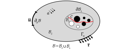
Figure 1: Setup of the notation: the unbroken domain is denoted by ${\mathcal{B}}_{C}$ and $\mathcal{C}$ is the crack phase-field. The smeared crack phase-field is approximated by the domain ${\mathcal{B}}_{L}$. The whole domain is defined as a close subset as ${{\mathcal{B}}:=\bar{{\mathcal{B}}}_{C}\cup\bar{{\mathcal{B}}}_{L}}$. The fracture boundary is $\partial{\mathcal{B}}_{L}$ and the outer boundary of the domain is $\partial{\mathcal{B}}$.

2.2 .Variational formulation for the multi-field problem

In this section, we recapitulate a variational approach to brittle fracture in elastic solids at small strains. The energy stored in a bulk strain density for isotropic materials is characterized by the three invariants,

$$I_{1}(\bm{\varepsilon})=tr(\bm{\varepsilon})\quad,\quad I_{2}(\bm{\varepsilon})=tr(\bm{\varepsilon}^{2})\quad,\quad I_{3}(\bm{\varepsilon})=tr(\bm{\varepsilon}^{3}).$$ (2)

Additionally, it is assumed that the solid material is reinforced by only one family of fibers which is denoted as transversely isotropic material. A single preferred direction at point ${\bm{\mathnormal{x}}}$ is defined by the normal vector $\bm{a}(\bm{x})$ with $\|{\bm{\mathnormal{a}}}\|=1$ that is called structural director. This type of material has the highest strength in the direction of the fiber and depicts isotropic response along its orthogonal direction. Hence, the stress state at a material point $\bm{x}$ depends on the deformation and the given single preferred direction. Thus it results to a deformation-direction-dependent problem. To do so, a penalty-like parameter $\chi>0$ is defined to restrict a deformation on the normal plane to ${\bm{\mathnormal{a}}}$. The effective bulk free energy now depends on two second-order tensorial quantities, namely the strain $\bm{\varepsilon}$ and structural ${\bm{\mathnormal{M}}}$ tensor, defined as

$${\bm{\varepsilon}}=\nabla_{s}{\bm{\mathnormal{u}}}=\mathop{\operator@font sym}[\nabla{\bm{\mathnormal{u}}}]\quad\mathchoice{\hbox{{and}}}{\hbox{{and}}}{\hbox{{and}}}{\hbox{{and}}}\quad{\bm{\mathnormal{M}}}:={\bm{\mathnormal{a}}}\otimes{\bm{\mathnormal{a}}},$$ (3)

they can be represented by additional two deformation-direction-dependent invariants

$$I_{4}(\bm{\varepsilon};{\bm{\mathnormal{M}}})=tr(\bm{\varepsilon.M})=\|{\bm{\mathnormal{a}}}\|_{\bm{\varepsilon}}^{2}=\lambda_{a_{0}}^{2}\quad,\quad I_{5}(\bm{\varepsilon};{\bm{\mathnormal{M}}})=tr(\bm{\varepsilon}^{2}.\bm{M}).$$ (4)

Note, that $I_{4}$ is nothing else than the quadratic stretch in the direction ${\bm{\mathnormal{a}}}$ of the fiber. Let the effective strain density function, ${\Psi}(\bm{\varepsilon};{\bm{\mathnormal{M}}})$ possesses the property of the transversely isotropic material which has the coordinate-free representation for both matrix and fiber materials. Thus the following holds

$${\Psi}(\bm{\varepsilon};{\bm{\mathnormal{M}}})=:{\Psi}({\bm{\mathnormal{Q}}}\bm{\varepsilon}{\bm{\mathnormal{Q}}}^{T};{\bm{\mathnormal{Q}}}{\bm{\mathnormal{M}}}{\bm{\mathnormal{Q}}}^{T})\quad\forall{\bm{\mathnormal{Q}}}\in{\mathcal{G}}\subset{\mathcal{O}}(3),$$ (5)

that holds for all orthogonal tensor ${\bm{\mathnormal{Q}}}$, i.e. ${\bm{\mathnormal{Q}}}^{T}{\bm{\mathnormal{Q}}}={\bm{\mathnormal{Q}}}{\bm{\mathnormal{Q}}}^{T}={\bm{\mathnormal{I}}}$, that is a subset of the symmetry group ${\mathcal{G}}$ of the anisotropic material. ${\bm{\mathnormal{I}}}=\delta_{ij}$ is the second order identity tensor. We denote that ${\Psi}(\bm{\varepsilon};{\bm{\mathnormal{M}}})$ is a scalar-valued isotropic tensor function of the symmetric strain tensor $\bm{\varepsilon}$ and the structural tensor ${\bm{\mathnormal{M}}}$. Hence, the scalar-valued effective strain density function is an invariant in space and time between two pairs of point in the given domain under rotation. Thus ${\Psi}(\bm{\varepsilon};{\bm{\mathnormal{M}}})$ can be represented by the principal invariants of $\bm{\varepsilon}$ and ${\bm{\mathnormal{M}}}$ as

$${\Psi}(\bm{\varepsilon};{\bm{\mathnormal{M}}}) ={\Psi}\big{(}I_{1}(\bm{\varepsilon}),I_{2}(\bm{\varepsilon}),I_{4}(\bm{\varepsilon};{\bm{\mathnormal{M}}}),I_{5}(\bm{\varepsilon};{\bm{\mathnormal{M}}})\big{)}$$ (6)

$$=\widetilde{\Psi}^{iso}\big{(}I_{1}(\bm{\varepsilon}),I_{2}(\bm{\varepsilon})\big{)}+\widetilde{\Psi}^{aniso}\big{(}I_{4}(\bm{\varepsilon};{\bm{\mathnormal{M}}}),I_{5}(\bm{\varepsilon};{\bm{\mathnormal{M}}})\big{)}.$$

Herein, the isotropic free-energy function corresponds to

$$\widetilde{\Psi}^{iso}\big{(}I_{1}(\bm{\varepsilon}),I_{2}(\bm{\varepsilon})\big{)}:=\frac{\lambda}{2}I^{2}_{1}+\mu I_{2},$$ (7)

with $\lambda>0$ and $\mu>0$ being the elastic Lamé constants. The anisotropic free-energy function is defined as

$$\widetilde{\Psi}^{aniso}\big{(}I_{4}(\bm{\varepsilon};{\bm{\mathnormal{M}}}),I_{5}(\bm{\varepsilon};{\bm{\mathnormal{M}}})\big{)}:=\frac{1}{2}\chi I^{2}_{4}+2\,{\Xi}\,I_{5},$$ (8)

with the anisotropic material parameters $\chi$ and $\Xi$. A stress-free condition, i.e. $\bm{\varepsilon}=0$, is required $\widetilde{\Psi}^{iso}\big{(}I_{1}(\bm{0}),I_{2}(\bm{0})\big{)}=0$. Moreover, $\widetilde{\Psi}^{aniso}\big{(}I_{4}(\bm{0};{\bm{\mathnormal{M}}}),I_{5}(\bm{0};{\bm{\mathnormal{M}}})\big{)}=0$ must hold true.

Using these definitions, to establish variational based anisotropic phase-field approach to brittle fractures, we define the bulk free energy functional which represents the stored energy in bulk as

$$\mathcal{E}_{bulk}({\bm{\mathnormal{u}}};{\bm{\mathnormal{M}}})=\int_{{\mathcal{B}}_{C}}{\Psi}(\bm{\varepsilon};{\bm{\mathnormal{M}}})\mathrm{d}{\bm{x}}-\int_{{\partial_{N}{\mathcal{B}}_{C}}}{\bm{\bar{\tau}}}\cdot\bm{u}\,\mathrm{d}s.$$ (9)

Herein, $\bm{\bar{\tau}}$ denotes the traction forces on the complementary boundaries ${\partial_{N}{\mathcal{B}}_{C}:=\Gamma_{N}\cup\mathcal{C}}$.

The total energetic functional is based on both the stored bulk energy as well as the fracture dissipation, defined in the work of [30],

$$\mathcal{E}({\bm{\mathnormal{u}}},\mathcal{C};{\bm{\mathnormal{M}}})=\mathcal{E}_{bulk}({\bm{\mathnormal{u}}};{\bm{\mathnormal{M}}})+G_{c}\mathcal{H}^{\delta-1}(\mathcal{C})\,,$$ (10)

where $G_{c}$ is the Griffith’s critical elastic energy release rate and $\mathcal{H}^{\delta-1}$ is a $\delta-1$ dimensional Hausdorff measure. For the numerical treatment we regularize Eq. 10 following [17]. Specifically, the crack energy is approximated through a sequence of elliptic problems, so-called Ambrosio-Tortorelli functionals, see [7, 8]. Therein, $\mathcal{H}^{\delta-1}$ is regularized by the crack phase-field $d$. Finally, we account for the crack irreversibility constraint meaning the crack can only grow:

$$\dot{d}\leq 0.$$ (11)

In the incremental version, this condition reads:

$$d\leq d^{old},$$

where $d:=d(t_{n})$ and $d^{old}:=d(t_{n-1})$. For stating the variational formulations, we now introduce:

$$\bm{V} :=\{{\bf H}^{1}({\mathcal{B}})^{\delta}:\bm{u}=\bar{\bm{u}}\;\mathrm{on}\;\partial_{D}{\mathcal{B}}\},\quad W:=\text{H}^{1}({\mathcal{B}}),$$ (12)

$$W_{in} :=\{d\in\text{H}^{1}({\mathcal{B}})^{\delta-1}|\;0\leq d\leq d^{old}\}.$$

As typical in problems with inequality constraints (see e.g., [51, 52]), $W_{in}$ is a nonempty, closed, convex, subset of the linear function space $W$. Due to the inequality constraint in Eq. 11, $W_{in}$ is no longer a linear space.

2.3 .Phase-field approximation of anisotropic crack topologies

The variational approach of [18] is widely used for fracture failure phenomena in isotropic elastic solids. As a point of departure, in line with [67, 23], let a regularized macro crack topology of a sharp crack be represented by the exponential function $1-\exp^{[-|x|/l]}$ satisfying $d(0)=0$. We define a regularized isotropic crack surface energy functional of the solid by,

$$G_{c}\mathcal{H}^{\delta-1}_{iso}(\mathcal{C}):=G_{c}\int_{\mathcal{B}}\gamma^{iso}_{l}(d,\nabla d)\,\mathrm{d}{{\bm{\mathnormal{x}}}}\quad\mathchoice{\hbox{{with}}}{\hbox{{with}}}{\hbox{{with}}}{\hbox{{with}}}\quad\gamma^{iso}_{l}(d,\nabla d):=\frac{1}{2l}{(1-d)^{2}}+\frac{l}{2}\nabla d.\nabla d,$$ (13)

in terms of the isotropic crack surface density function per unit volume of the solid $\gamma^{iso}_{l}$.

The above representation of a crack surface density function is extended for the class of anisotropic responses; as for instance outlined in [78, 88, 76]. Similarly to the deformation field, we define a total crack surface density function. It is additively decomposed into an isotropic and anisotropic crack surface density function, respectively, as follows

$$\gamma_{l}(d,{\bm{\mathnormal{Q}}}\nabla d):=\gamma^{iso}_{l}(d,\nabla d)+\gamma^{aniso}_{l}(\nabla d)\quad\mbox{for all}\quad{\bm{\mathnormal{Q}}}\in{\mathcal{G}}\subset{\mathcal{O}}(3),$$ (14)

where ${\mathcal{G}}$ is a given symmetry group of the anisotropic material, i.e. the set of rotation and reflection vectors, and $\gamma^{aniso}_{l}(d,\nabla d)$ represents an augmented crack surface density for the anisotropic response. Let this function posses the property of the transversely isotropic material which has the coordinate-free representation for both matrix and fibers materials. This leads to

$$\gamma_{l}(d,\nabla d;{\bm{\mathnormal{M}}})=\gamma_{l}(d^{2},\nabla d\cdot\nabla d,\nabla d\cdot{\bm{\mathnormal{M}}}\cdot\nabla d)\;.$$ (15)

Using this definition, an anisotropic crack surface density response can be defined as

$$\gamma^{aniso}_{l}(\nabla d;{\bm{\mathnormal{M}}}):=\alpha\frac{l}{2}\nabla d.{\bm{\mathnormal{M}}}.\nabla d.$$ (16)

This type of fracture function has the highest geometric resistance in the fiber direction and has an isotropic response along its orthogonal direction. Hence, the geometric resistance state at a material point $\bm{x}$ depends on crack phase-field and the given single preferred direction $\bm{a}$. This results in a crack-direction-dependent problem.

The anisotropic term $\alpha$ in Eq. 16 behaves as a penalty-like parameter and hence for $\alpha\rightarrow\infty$ one obtains $\nabla d\cdot{\bm{\mathnormal{a}}}=0$, which means that the crack lies parallel to the preferred orientation. For $\alpha\rightarrow 0$ the isotropic response will be recovered.

Formulation 2.1 (Energy functional for the anisotropic crack topology).

Let ${\bm{\mathnormal{M}}}$, $\chi$, $\Xi$ and $\alpha$ be given with the initial conditions $\bm{u}_{0}=\bm{u}(\bm{x},0)$ and $d_{0}=d(\bm{x},0)$. For the loading increments $n=1,2,\ldots,N$, find $\bm{u}:=\bm{u}^{n}\in V$ and $d:=d^{n}\in W_{in}$ such that the functional

$$\mathcal{E}({\bm{u}},d;{\bm{\mathnormal{M}}}) :=\mathcal{E}_{bulk}(\bm{u},d_{+};{\bm{\mathnormal{M}}})+\;\mathcal{E}_{frac}(d;{\bm{\mathnormal{M}}})+\;\mathcal{E}_{ext}(\bm{u})$$

$$\>=\int_{{\mathcal{B}}}w_{bulk}(\bm{\varepsilon},d;{\bm{\mathnormal{M}}})\mathrm{d}{\bm{x}}+\int_{\mathcal{B}}w_{frac}(d,\nabla d;{\bm{\mathnormal{M}}})\,\mathrm{d}{\bm{x}}-\int_{\partial_{N}{\mathcal{B}}}{\bm{\bar{\tau}}}\cdot\bm{u}\,\mathrm{d}s,$$

is minimized. The elastic bulk density $w_{bulk}$ along with the fracture contribution $w_{frac}$ both define the so-called total pseudo-energy density function as

$$w({\bm{\varepsilon}},d,\nabla d;{\bm{\mathnormal{M}}})=w_{bulk}({\bm{\varepsilon}},d;{\bm{\mathnormal{M}}})+w_{frac}(d,\nabla d;{\bm{\mathnormal{M}}}),$$

$$w_{bulk}({\bm{\varepsilon}},d;{\bm{\mathnormal{M}}})=g(d_{+}){\Psi}(\bm{\varepsilon};{\bm{\mathnormal{M}}}),$$

$$w_{frac}(d,\nabla d;{\bm{\mathnormal{M}}})=G_{c}\gamma_{l}(d,\nabla d;{\bm{\mathnormal{M}}}).$$

Remark 2.1.

In the case of elastic cracks, it can be shown that the phase field satisfies $0\leq d\leq 1$. When additional physics are included for instance a fluid inside the fracture [74] or non-isothermal effects [79], the energy functional must be modified to cope with negative values of $d$. Hence in order to allow for future extensions, we work in the remainder of this paper with $d_{+}$ rather than $d$. A detailed discussion is provided in [74][Section 3].

Remark 2.2.

The comparison of the bulk energy functional in Eq. 10 and Formulation 2.1 is tow-fold. First, the integration is changed from ${\mathcal{B}}_{C}$ to the entire domain ${\mathcal{B}}$ due to the presence of the phase-field function $d$. Second, the presence of $d$ in the bulk energy through the degradation function $g(d)$ defines the transition state from the unbroken to fracture state hence results in the degradation of the solid material as well as the crack propagation.

2.4 .Strain-energy decomposition

Since the fracturing material behaves quite differently in tension and compression, a consistent split for the strain energy density function is employed, where we apply the decomposition only to the isotropic strain energy function, i.e. ${\Psi}^{iso}\big{(}I_{1}(\bm{\varepsilon}),I_{2}(\bm{\varepsilon})\big{)}$. Hence, instead of dealing directly with $\bm{\varepsilon}(\bm{u})$, we perform additive decomposition of the strain tensor as

$$\bm{\varepsilon}(\bm{u})=\bm{\varepsilon}^{+}(\bm{u})+\bm{\varepsilon}^{-}(\bm{u})\quad\mathchoice{\hbox{{with}}}{\hbox{{with}}}{\hbox{{with}}}{\hbox{{with}}}\quad\bm{\varepsilon}^{\pm}(\bm{u}):=\sum_{i=1}^{\delta}\langle\varepsilon_{i}\rangle^{\pm}{\textbf{N}_{i}}\otimes{\textbf{N}_{i}}\ ,$$

with the tension $\bm{\varepsilon}^{+}$ and compression $\bm{\varepsilon}^{-}$ strains. Here, $\langle x\rangle_{\pm}:=\frac{x{\pm}|x|}{2}$ is a ramp function of $\mathbb{R}_{\pm}$ expressed by the Macauley bracket. $\{\varepsilon_{i}\}$ are the principal strains and $\{\textbf{N}_{i}\}$ are the principal strain directions. The tension/compression fourth-order projection tensor is defined as

$$\mathbb{P}^{\pm}_{\bm{\varepsilon}}:=\frac{\partial\bm{\varepsilon}^{\pm}}{\partial\bm{\varepsilon}}=\frac{\partial\big{(}\sum_{i=1}^{\delta}\langle\varepsilon_{i}\rangle^{\pm}{\textbf{N}_{i}}\otimes{\textbf{N}_{i}}\big{)}}{\partial\bm{\varepsilon}}\ .$$ (17)

It turns out that, $\mathbb{P}^{\pm}_{\bm{\varepsilon}}$ projects the total strain into its positive and negative parts accordingly, i.e $\bm{\varepsilon}^{\pm}=\mathbb{P}^{\pm}_{\bm{\varepsilon}}:\bm{\varepsilon}$. So, a decoupled representation of the strain-energy function into a so-called tension and compression contribution is given as follows,

$${\Psi}^{iso}\big{(}I_{1}(\bm{\varepsilon}),I_{2}(\bm{\varepsilon})\big{)}:=\underbrace{\widetilde{\Psi}^{iso,+}\big{(}I^{+}_{1}(\bm{\varepsilon}),I^{+}_{2}(\bm{\varepsilon})\big{)}}_{\text{tension term}}+\underbrace{\widetilde{\Psi}^{iso,-}\big{(}I^{-}_{1}(\bm{\varepsilon}),I^{-}_{2}(\bm{\varepsilon})\big{)}}_{\text{compression term}}.$$ (18)

Herein, the positive and negative principal invariants are

$$I_{1}^{\pm}(\bm{\varepsilon}):=\langle{I_{1}(\bm{\varepsilon})}\rangle_{\pm},\quad I^{\pm}_{2}(\bm{\varepsilon}):=I_{2}(\bm{\varepsilon}^{\pm}).$$ (19)

Remark 2.3.

An alternative definition to $I_{1}^{\pm}(\bm{\varepsilon}):=\langle{I_{1}(\bm{\varepsilon})}\rangle_{\pm}$, can be defined by using the same description introduced in $I_{2}^{\pm}(\bm{\varepsilon})$ for the first principal invariant which results in $I^{\pm}_{1}(\bm{\varepsilon}):=I_{1}(\bm{\varepsilon}^{\pm})$. This provides a new description for the strain-energy function represented in Eq. 18. However, that is beyond the scope of present paper and will investigated in future work.

Physically, it is trivial to assume that the degradation induced by the phase field acts only on the tensile and shear counterpart of the elastic strain density function. Hence, it is that assumed there is no degradation in compression, which also prevents interpenetration of the crack lips during crack closure, see [67]. It turns out that the bulk work density function for the fracturing material becomes,

$$w_{bulk}({\bm{\varepsilon}},d;{\bm{\mathnormal{M}}}):=g(d_{+})\Big{[}\widetilde{\Psi}^{iso,+}(I^{+}_{1},I^{+}_{2})+\widetilde{\Psi}^{aniso}(I_{4},I_{5})\Big{]}+\widetilde{\Psi}^{iso,-}(I^{-}_{1},I^{-}_{2}).$$ (20)

Here a monotonically decreasing quadrature degradation function, i.e.

$$g(d_{+}):=(1-\kappa)d_{+}^{2}+\kappa,$$ (21)

describes the degradation of the solid with the evolving crack phase-field parameter $d$. The small residual stiffness $\kappa$ is introduced to prevent numerical problems. The constitutive stress response corresponding to Eq. 20 reads

$${\bm{\sigma}}(\bm{\varepsilon},d;{\bm{\mathnormal{M}}}):=\frac{\partial w_{bulk}({\bm{\varepsilon}},d;{\bm{\mathnormal{M}}})}{\partial{\bm{\varepsilon}}}=\bm{\sigma}_{\bm{\varepsilon}}^{iso}+\bm{\sigma}_{\bm{\varepsilon}}^{aniso},$$ (22)

$$\bm{\sigma}_{\bm{\varepsilon}}^{iso}=g(d_{+})\frac{\partial\widetilde{\Psi}^{iso,+}}{\partial\bm{\varepsilon}}+\frac{\partial\widetilde{\Psi}^{iso,-}}{\partial\bm{\varepsilon}}=g(d_{+}){\bm{\widetilde{\sigma}}^{iso,+}_{\bm{\varepsilon}}}+{\bm{\widetilde{\sigma}}^{iso,-}_{\bm{\varepsilon}}},$$

$$\bm{\sigma}_{\bm{\varepsilon}}^{aniso}=g(d_{+})\frac{\partial\widetilde{\Psi}^{aniso}}{\partial\bm{\varepsilon}}=g(d_{+}){\bm{\widetilde{\sigma}}^{aniso}_{\bm{\varepsilon}}},$$

with,

$$\bm{\widetilde{\sigma}}_{\bm{\varepsilon}}^{iso,\pm}:=\lambda I_{1}^{\pm}(\bm{\varepsilon}){\textbf{I}}+2\mu\bm{\varepsilon}_{\pm}\quad\mathchoice{\hbox{{and}}}{\hbox{{and}}}{\hbox{{and}}}{\hbox{{and}}}\quad{\bm{\widetilde{\sigma}}^{aniso}_{\bm{\varepsilon}}}=\chi I_{4}{\bm{\mathnormal{M}}}+2\,\Xi\,({\bm{\varepsilon}}\cdot{\bm{\mathnormal{M}}}+{\bm{\mathnormal{M}}}\cdot{\bm{\varepsilon}})$$ (23)

Formulation 2.2 (Energy functional for the anisotropic crack topology).

Let ${\bm{\mathnormal{M}}}$, $\chi$, $\Xi$ and $\alpha$ be given with the initial conditions $\bm{u}_{0}=\bm{u}(\bm{x},0)$ and $d_{0}=d(\bm{x},0)$. For the loading increments $n=1,2,\ldots,N$, find $\bm{u}:=\bm{u}^{n}\in V$ and $d:=d^{n}\in W_{in}$ such that the functional

$$\mathcal{E}({\bm{u}},d;{\bm{\mathnormal{M}}}) =\underbrace{\int_{\mathcal{B}}\big{[}g(d_{+})\widetilde{\Psi}^{iso,+}+\widetilde{\Psi}^{iso,-}\big{]}\mathrm{d}{\textbf{x}}}_{\text{matrix deformation term}}+\underbrace{\int_{\mathcal{B}}g(d_{+})\widetilde{\Psi}^{aniso}\mathrm{d}{\textbf{x}}}_{\text{fiber deformtion term}}$$

$$+G_{c}\underbrace{\int_{\mathcal{B}}\gamma^{iso}_{l}\mathrm{d}{\textbf{x}}}_{\text{matrix fracture term}}+G_{c}\underbrace{\int_{\mathcal{B}}\gamma^{aniso}_{l}\mathrm{d}{\textbf{x}}}_{\text{fiber fracture term}}-\underbrace{\int_{\partial_{N}{\mathcal{B}}}{\bm{\bar{\tau}}}\cdot\bm{u}\,\mathrm{d}s}_{\text{external load}},$$

is minimized.

The minimization problem for the given energy functional of the anisotropic crack topology in Formulation 2.2 takes the following compact form:

$$\framebox{$\displaystyle\{\bm{u},d\}=\mbox{arg}\{\;\mathop{\operator@font\mbox{min}}\limits_{\vbox{\halign{\ifx cc\hfil\fi\ifx rc\hfil\fi$\m@th\scriptstyle#$\ifx cc\hfil\fi\ifx lc\hfil\fi\cr\bm{u}\in\bf{V}\crcr}}}\mathop{\operator@font\mbox{min}}\limits_{\vbox{\halign{\ifx cc\hfil\fi\ifx rc\hfil\fi$\m@th\scriptstyle#$\ifx cc\hfil\fi\ifx lc\hfil\fi\cr d\in W_{in}\crcr}}}\,[\;\mathcal{E}(\bm{u},d;{\bm{\mathnormal{M}}})\;]\;\}.$}$$ (24)

The stationary points of the energy functional in Formulation 2.2 are characterized by the first-order necessary conditions, namely the so-called Euler-Lagrange equations, which are obtained by differentiation with respect to ${\bm{u}}$ and $d$.

Formulation 2.3 (Euler-Lagrange equations).

Let ${\bm{\mathnormal{M}}}$, $\chi$, $\Xi$ and $\alpha$ be given with the initial conditions $\bm{u}_{0}=\bm{u}(\bm{x},0)$ and $d_{0}=d(\bm{x},0)$. For the loading increments $n=1,2,\ldots,N$, find $\bm{u}:=\bm{u}^{n}\in V$ and $d:=d^{n}\in W_{in}:$

$${\mathcal{E}}_{\bm{u}}(\bm{u},d;\delta\bm{u})=\int_{\mathcal{B}}g(d_{+}){\bm{\widetilde{\sigma}}^{iso,+}_{\bm{\varepsilon}}}(\bm{u}):{\bm{\varepsilon}}(\delta\bm{u})\mathrm{d}{\textbf{x}}+\int_{\mathcal{B}}{\bm{\widetilde{\sigma}}^{iso,-}_{\bm{\varepsilon}}(\bm{u})}:{\bm{\varepsilon}}(\delta\bm{u})\mathrm{d}{\textbf{x}}$$ (25)

$$\qquad\qquad\;\;+\int_{\mathcal{B}}g(d_{+}){\bm{\widetilde{\sigma}}^{aniso}_{\bm{\varepsilon}}}(\bm{u}):{\bm{\varepsilon}}(\delta\bm{u})\mathrm{d}{\textbf{x}}-\int_{\partial_{N}{\mathcal{B}}}{\bm{\bar{\tau}}}\cdot{\delta\bm{u}}\,\mathrm{d}s=0\quad\forall{\delta\bm{u}}\in V,$$

$${\mathcal{E}}_{d}(\bm{u},d;\delta d-d)=(1-\kappa)\int_{\mathcal{B}}d_{+}\big{[}{\bm{\widetilde{\sigma}}^{iso,+}_{\bm{\varepsilon}}}(\bm{u})+{\bm{\widetilde{\sigma}}^{aniso}_{\bm{\varepsilon}}}(\bm{u})\big{]}:{\bm{\varepsilon}}(\bm{u}).(\delta d-d)\mathrm{d}{\textbf{x}}$$

$$\qquad\qquad\qquad\qquad+G_{c}\int_{\mathcal{B}}\left(\frac{1}{l}(d-1).(\delta d-d)+l\nabla d.\nabla(\delta d-d)\right)\mathrm{d}{\textbf{x}}$$

$$\qquad\qquad\qquad\qquad+G_{c}\int_{\mathcal{B}}\alpha l\nabla d.{\bm{\mathnormal{M}}}.\nabla(\delta d-d)\,\mathrm{d}{{\bm{\mathnormal{x}}}}\geq 0\quad\forall\delta d\in W\cap L^{\infty}.$$

${\mathcal{E}}_{\bm{u}}$ and ${\mathcal{E}}_{d}$ are the directional derivatives of the energy functional with respect to $\bm{u}$ and $d$, respectively. Furthermore, $\delta\bm{u}\in\{{\bf H}^{1}({\mathcal{B}})^{\delta}:\delta\bm{u}=\bm{0}\;\mathrm{on}\;\partial_{D}{\mathcal{B}}\}$ is the deformation test function and $\delta d\in H^{1}({\mathcal{B}})$ is the phase-field test function.

2.5 .The Euler-Lagrange equations in a strong form

In order to complete our derivations, the strong form of Formulation 2.3 will be derived in this section. Using integration by parts, we obtain a quasi-stationary elliptic system for the displacements and the phase-field variable, where the latter one is subject to an inequality constraint in time and therefore needs to be complemented with a complementary condition:

Formulation 2.4 (Strong form of the Euler-Lagrange equations).

Let ${\bm{\mathnormal{M}}}$, $\chi$, $\Xi$ and $\alpha$ be given with the initial conditions $\bm{u}_{0}=\bm{u}(\bm{x},0)$ and $d_{0}=d(\bm{x},0)$. For the loading increments $n=1,2,\ldots,N$, we solve a displacement equation where we seek $\bm{u}:=\bm{u}^{n}:{\mathcal{B}}\rightarrow\mathbb{R}^{d}$ such that

$$-\mathop{\operator@font div}({\bm{\sigma}})={\bm{\mathit{0}}}\quad in\;{\mathcal{B}},$$

$${\bm{u}}=\bar{}{\bm{\mathnormal{u}}}\quad on\;\partial_{D}{\mathcal{B}},$$

$${\bm{\sigma}}\cdot{\bm{\mathnormal{n}}}=\bar{{\bm{\tau}}}\quad on\;\partial_{N}{\mathcal{B}},$$

in terms of the stress tensor ${\bm{\sigma}}$ defined in Eq. 22 and the given displacement field $\bar{}{\bm{\mathnormal{u}}}$. The phase-field system consists of four parts: the PDE, the inequality constraint and a compatibility condition (in fracture mechanics called Rice condition [84]) along with the Neumann-type boundary conditions. Find $d:=d^{n}:{\mathcal{B}}\rightarrow[0,1]$ such that

$$-\Big{(}2(1-\kappa)d_{+}\big{[}\widetilde{\Psi}^{iso,+}+\widetilde{\Psi}^{aniso}\big{]}-\frac{G_{c}}{l}(1-d)-G_{c}l\Delta d-G_{c}\alpha l\mathop{\operator@font div}(\nabla d.{\bm{\mathnormal{M}}})\Big{)}\geq\;0\quad in\;{\mathcal{B}},$$

$$\dot{d}\leqslant 0\quad in\;{\mathcal{B}},$$

$$-\Big{(}2(1-\kappa)d_{+}\widetilde{\Psi}^{iso,+}(\bm{\varepsilon}(\bm{u}))-\frac{G_{c}}{l}(1-d)-G_{c}l\Delta d-G_{c}\alpha l\mathop{\operator@font div}(\nabla d.{\bm{\mathnormal{M}}})\Big{)}\;\dot{d}=0\quad in\;{\mathcal{B}},$$

$$\;({\textbf{I}}+\alpha{\bm{\mathnormal{M}}}){\nabla d\cdot{\bm{\mathnormal{n}}}}=0\quad on\;\partial{\mathcal{B}}.$$

The mentioned inequality minimization problem for the phase-field equation can be resolved through: (a) fixing the fracture with Dirichlet conditions [17], (b) Penalty method, see [73] (including a mathematical analysis), (c) an Augumented Lagragian penalization see [92], (d) Primal-dual active set method; see [42, 54], (e) Maximum crack driving state function, see [67, 70]. In the present work, we consider the maximum crack driving state function to prevent the crack healing by having a positive crack dissipation known as irreversibility criteria and given in details in next section.

2.6 .Crack driving force

In this section, a formulation for the crack phase-field PDE equation in Formulation 2.4 is reformulated based on the crack driving force. A thermodynamical consistency for the preservation of the energy balance due to the fracture dissipation results to the Karush-Kuhn-Tucker form, see [69]. As a point of departure, the modular structure of the anisotropic phase-field fracture equation assumes the following form

$$\underbrace{\eta\dot{d}}_{{crack\,\,update}}=\underbrace{-g^{\prime}(d_{+})\widetilde{D}}_{crack\,\,driving\,\,force}-\underbrace{l\delta_{d}\gamma_{l}}_{resistance}\leq 0,$$ (26)

as outlined in the works of Miehe and coworkers [70, 69, 4, 5]. Here, $\widetilde{D}$ is a crack driving state function which depends on a $state$ array of strain- or stress like quantities. To get rid of the above inequality evolution problem, we maximize the inequality equation given in (26) for the full process history $s\in[0,t_{n}]$,

$$-g^{\prime}(d_{+})\displaystyle\max\limits_{\vbox{\halign{\ifx cc\hfil\fi\ifx rc\hfil\fi$\m@th\scriptstyle#$\ifx cc\hfil\fi\ifx lc\hfil\fi\cr s\in[0,t_{n}]\crcr}}}\widetilde{D}=l\delta_{d}\gamma_{l}\;.$$ (27)

We introduce maximum positive crack driving force ${\mathcal{H}}$ in $t\in[0,t_{n}]$ denoted as,

$${\mathcal{H}}({\bm{\mathnormal{x}}},t):=\displaystyle\max\limits_{\vbox{\halign{\ifx cc\hfil\fi\ifx rc\hfil\fi$\m@th\scriptstyle#$\ifx cc\hfil\fi\ifx lc\hfil\fi\cr{s}\in[0,t_{n}]\crcr}}}\widetilde{D}\big{(}state({\bm{\mathnormal{x}}},{\bm{\varepsilon}}(s))\big{)},$$ (28)

and hence (26) can be restated as,

$$\framebox{$\displaystyle\underbrace{\eta\dot{d}}_{{crack\,\,update}}=\underbrace{-g^{\prime}(d_{+}){\mathcal{H}}}_{max\,\,crack\,\,driving\,\,force}-\underbrace{l\delta_{d}.\gamma_{l}}_{resistance}.$}$$ (29)

Depending on the type of the crack driving state function which can be either without or with threshold, $\widetilde{D}$ can take different description, see [1, 2, 3]. The crack phase-field evolution in (29) is defined in the domain ${\mathcal{B}}$ that is augmented with an imposed Neumann homogeneous boundary condition as

$${({\textbf{I}}+\alpha{\bm{\mathnormal{M}}}){\nabla d\cdot{\bm{\mathnormal{n}}}}=0}\quad on\;\partial{\mathcal{B}}.$$ (30)

Note, that in Eq. 26 the rate-independent case is recovered for $\eta\rightarrow 0$, where the crack topology is then simply determined by an equilibrium between the crack driving force and the geometric crack resistance. These equations are interpreted as generalized Ginzburg-Landau-type evolution equations for the crack phase-field $d$. Equation 29 restated for the rate-independent limit $\eta\rightarrow 0$ to the so-called Karush-Kuhn-Tucker form:

$$\framebox{$\displaystyle\dot{d}\leqslant 0;\quad-\delta_{d}w\;\geq\;0,\quad\dot{d}\,[-\delta_{d}w]=0.$}$$ (31)

This condition provides a natural assumption due to the positive fracture dissipation know as crack irreversibility condition. The latter constraint is ensured by a specific constitutive assumption that relates the functional derivative to a positive energetic driving force. The last condition in (31) is the balance law for the evolution of the crack phase-field which ensures the principal of maximum dissipation during the crack phase-field evolution (see e.g. [67]). It is known as compatibility condition.

Remark 2.4.

Karush-Kuhn-Tucker stated in (31) along with (30) are the modular structure of the Euler-Lagrange equations in a strong form which are given in Formulation 2.4.

By defining the maximum positive crack driving force ${\mathcal{H}}$ in terms of the the crack driving state function $\widetilde{D}$ at hand, Formulation 2.3 can be stated as an equality minimization. Thus ${\mathcal{H}}$ substitutes the corresponding $\big{[}\widetilde{\Psi}^{iso,+}+\widetilde{\Psi}^{aniso}\big{]}$ term in the original $\mathcal{E}_{d}$. To derive the crack driving state function we recall the irreversibly inequality condition, i.e. $\dot{d}\leq 0$. It follows that the left hand side of (26) has to be always positive to avoid the crack healing process

$$-\delta_{d}w=(\kappa-1)2d_{+}\big{[}\widetilde{\Psi}^{iso,+}+\widetilde{\Psi}^{aniso}\big{]}-G_{c}\delta_{d}\gamma_{l}(d,\nabla d;{\bm{\mathnormal{M}}})\leqslant 0.$$ (32)

Maximization of this inequality in the full process history $s\in[0,t_{n}]$, yields

$$(\kappa-1)2d_{+}\displaystyle\max\limits_{\vbox{\halign{\ifx cc\hfil\fi\ifx rc\hfil\fi$\m@th\scriptstyle#$\ifx cc\hfil\fi\ifx lc\hfil\fi\cr s\in[0,t_{n}]\crcr}}}\big{[}\widetilde{\Psi}^{iso,+}+\widetilde{\Psi}^{aniso}\big{]}=G_{c}\delta_{d}\gamma_{l}(d,\nabla d;{\bm{\mathnormal{M}}}).$$ (33)

To follow the modular structure of the phase-field fracture equation defined in Eq. 26, we multiply (33) by $\frac{l}{G_{c}}$. With the definition of a positive crack driving force and shown by ${\mathcal{H}}$, hence (33) is restated as

$$(\kappa-1)2d_{+}{\mathcal{H}}=l\delta_{d}\gamma_{l}\;\;\mbox{if}\;{\mathcal{H}}:=\displaystyle\max\limits_{\vbox{\halign{\ifx cc\hfil\fi\ifx rc\hfil\fi$\m@th\scriptstyle#$\ifx cc\hfil\fi\ifx lc\hfil\fi\cr s\in[0,t_{n}]\crcr}}}\widetilde{D}\;\;\mbox{with}\;\;\widetilde{D}:=\frac{l\big{[}\widetilde{\Psi}^{iso,+}+\widetilde{\Psi}^{aniso}\big{]}}{G_{c}}.$$ (34)

It is evident that the crack driving state function given by (34) is directly effected by the regularization parameter $l$. Hence the crack driving state function has the property of length-scale dependency. The functional derivative of $\gamma_{l}$ with respect to $d$ is obtained as follows,

$$\int_{\mathcal{B}}\delta_{d}\gamma_{l}(d,\nabla d;{\bm{\mathnormal{M}}})\mathrm{d}{\bm{x}}:=\int_{\mathcal{B}}\bigg{(}\frac{\partial\gamma_{l}}{\partial d}+\frac{\partial\gamma_{l}}{\partial\nabla d}\bigg{)}\mathrm{d}{\bm{x}}=\int_{\mathcal{B}}\bigg{(}\frac{\partial\gamma_{l}}{\partial d}-\nabla.[\frac{\partial\gamma_{l}}{\partial\nabla d}]\bigg{)}\mathrm{d}{\bm{x}},$$ (35)

which leads to,

$$\int_{\mathcal{B}}\delta_{d}\gamma_{l}(d,\nabla d;{\bm{\mathnormal{M}}})\mathrm{d}{\bm{x}}=\int_{\mathcal{B}}\frac{1}{l}[(d-1)-l^{2}\Delta d-\alpha l^{2}\mathop{\operator@font div}(\nabla d.{\bm{\mathnormal{M}}})]\mathrm{d}{\bm{x}}.$$ (36)

Furthermore $\frac{\partial\gamma_{l}(d,\nabla d;{\bm{\mathnormal{M}}})}{\partial{\nabla d}}\cdot\bm{n}=({\textbf{I}}+\alpha{\bm{\mathnormal{M}}})l\nabla d\cdot\bm{n}=0$ refers to (30).

Formulation 2.5 (Final Euler-Lagrange equations).

Let ${\bm{\mathnormal{M}}}$, $\chi$, $\Xi$ and $\alpha$ be given with the initial conditions $\bm{u}_{0}=\bm{u}(\bm{x},0)$ and $d_{0}=d(\bm{x},0)$. For the loading increments $n=1,2,\ldots,N$, find $\bm{u}:=\bm{u}^{n}\in V$ and $d:=d^{n}\in W:$

$${\mathcal{E}}_{\bm{u}}(\bm{u},d_{+};\delta\bm{u})=\int_{\mathcal{B}}g(d_{+}){\bm{\widetilde{\sigma}}^{iso,+}_{\bm{\varepsilon}}}(\bm{u}):{\bm{\varepsilon}}(\delta\bm{u})\mathrm{d}{\textbf{x}}+\int_{\mathcal{B}}{\bm{\widetilde{\sigma}}^{iso,-}_{\bm{\varepsilon}}(\bm{u})}:{\bm{\varepsilon}}(\delta\bm{u})\mathrm{d}{\textbf{x}}$$ (37)

$$\qquad\qquad\;\;+\int_{\mathcal{B}}g(d_{+}){\bm{\widetilde{\sigma}}^{aniso}_{\bm{\varepsilon}}}(\bm{u}):{\bm{\varepsilon}}(\delta\bm{u})\mathrm{d}{\textbf{x}}-\int_{\partial_{N}{\mathcal{B}}}{\bm{\bar{\tau}}}\cdot{\delta\bm{u}}\,\mathrm{d}s=0\quad\forall{\delta\bm{u}}\in V,$$

$${\mathcal{E}}_{d}(\bm{u},d;\delta d)=(1-\kappa)\int_{\mathcal{B}}2d_{+}{\mathcal{H}}\delta d\mathrm{d}{\textbf{x}}$$

$$\qquad\qquad\qquad+\int_{\mathcal{B}}\Big{(}(d-1)\delta d+l^{2}\nabla d.\nabla\delta d\Big{)}\mathrm{d}{\textbf{x}}$$

$$\qquad\qquad\qquad+\int_{\mathcal{B}}\alpha l^{2}\nabla d.{\bm{\mathnormal{M}}}.\nabla\delta d\,\mathrm{d}{{\bm{\mathnormal{x}}}}=0\quad\forall\delta d\in W.$$

3 .Global-Local Formulation Applied to the Anisotropic Phase-Field Fracture

Departing point towards a Global-Local approach applied to the anisotropic phase-field formulation is the domain decomposition method [35]. We split the single-scale energy functional $\mathcal{E}$ indicated in Formulation 2.2 to the intact and fractured region, i.e. ${\mathcal{B}}_{C}$ and ${\mathcal{B}}_{L}$, respectively.

Accordingly, by introduction of the Fictitious domain ${\mathcal{B}}_{F}$, i.e. a coarse projection of the local domain into the global domain (later ${\mathcal{B}}_{G}$ refers to the global domain in Section 3.2), we extend the resulting non-overlapping domain decomposition formulation toward a Global-Local formulation applied to the anisotropic phase-field fracture. The Global-Local formulation applied to isotropic phase-field was first proposed by Gerasimov et al. [34]. The main objective was to introduce an adoption of the phase-field formulation within legacy codes, specifically for industrial applications.

An important definition for the subsequent treatment is the energy functional. We recall that the energy functional for the single-scale problem denoted as $\mathcal{E}$. We further define the energy functional for the domain decomposition by $\widehat{\mathcal{E}}$ and the Global-Local formulations as $\widetilde{\mathcal{E}}$.

3.1 .Non-overlapping domain decomposition formulation

Recall, the complementary domain ${\mathcal{B}}_{C}:={\mathcal{B}}\backslash{\mathcal{B}}_{L}\subset{\mathcal{B}}\in\mathbb{R}^{d}$ corresponds to the intact region and let ${\mathcal{B}}_{L}$ is an open domain, where the fracture surface is approximated in this region, see Fig. 2(a). It is assumed the fracture surface in ${\mathcal{B}}_{L}$ represents a reasonably small ’fraction’ of ${\mathcal{B}}$ such that $|{\mathcal{B}}_{L}|\ll|{\mathcal{B}}_{C}|$. We further define an interface between an unfractured domain ${\mathcal{B}}_{C}$ and fractured domain ${\mathcal{B}}_{L}$ by $\Gamma\in\mathbb{R}^{\delta-1}\subset{\mathcal{B}}$ in the continuum setting to be the interface between ${\mathcal{B}}_{L}$ and ${\mathcal{B}}_{C}$, such that ${\mathcal{B}}\equiv{\mathcal{B}}_{L}\cup\Gamma\cup{\mathcal{B}}_{C}$. We further assume that ${\mathcal{B}}_{L}$ is free from any externally imposed load and hence we have prescribed loads only in ${\mathcal{B}}_{C}$. Such an assumption is standard for the multi-scale setting, see [29].

Figure 2: Domain decomposition scheme. $(a)$ Geometry and loading setup of the single-scale boundary value problem. $(b)$ Non-overlapping domain decomposition setting whereas ${\mathcal{B}}$ is decomposed into the intact and fracture region denoted as complementary and local domains ${\mathcal{B}}_{L}$ and ${\mathcal{B}}_{C}$, respectively.

Consider a domain decomposition with geometric sketch in Fig. 2(b) applied to the single-scale domain plotted in Fig. 2(a). Two functions on ${\mathcal{B}}_{L}$ and ${\mathcal{B}}_{C}$ are considered, namely $\bm{u}_{L}\in{\bf{V}_{L}}$ and $\bm{u}_{C}\in{\bf{V}_{C}}$, where we introduce additional three sets:

$$\bm{V}_{L}:=\textbf{H}^{1}_{0}({\mathcal{B}}_{L})^{\delta},\quad{\bm{V}_{C}:={\bf{V}}({\mathcal{B}}_{C})},\quad\text{and}\;\;W_{L}:=W_{in}({\mathcal{B}}_{L})\;,$$

referring to the spaces defined in Eq. 12.

A descriptive motivation of the domain decomposition approach applied to the variational anisotropic phase-field modeling is related to two restriction in the model: (i) the strong coupling scheme that is the strong displacement continuity condition that holds along with (ii) the predefined interface. To this end, one needs to assume that the discrete interfaces for both complementary and local domain do exactly coincide in the strong sense, yielding

$$\bm{u}_{L}\overset{!}{=}\bm{u}_{C}\quad\mbox{at}\quad{\bm{x}}\in\Gamma=\Gamma_{C}=\Gamma_{L}.$$ (38)

This displacement continuity is often called primal approach in the literature, see e.g. [60].

Let the single-scale displacement field $\bm{u}\in{\bf V}$ be the solution of the multi-field variational problem in (24). It is decomposed as

$$\bm{u}(\bm{x},t):=\left\{\begin{tabular}[]{ll}$\bm{u}_{L}$&for ${{\bm{\mathnormal{x}}}}\in{\mathcal{B}}_{L}$,\\[2.84544pt] $\bm{u}_{C}$&for ${{\bm{\mathnormal{x}}}}\in{\mathcal{B}}_{C}$.\end{tabular}\right.$$ (39)

Since the fracture surface lives only in ${\mathcal{B}}_{L}$ we introduce scalar-valued function $d_{L}:{\mathcal{B}}_{L}\rightarrow[0,1]\in W_{L}$. The single-scale phase-field $d$ is then decomposed in the following form

$$d(\bm{x},t):=\left\{\begin{tabular}[]{ll}$d_{L}$&for ${{\bm{\mathnormal{x}}}}\in{\mathcal{B}}_{L}$,\\[2.84544pt] $1$&for ${{\bm{\mathnormal{x}}}}\in{\mathcal{B}}_{C}$.\end{tabular}\right.$$ (40)

By imposing (39) and (40) to the energy functional, indicated in Formulation 2.2, energy functionals corresponding to ${\mathcal{B}}_{C}$ and ${\mathcal{B}}_{L}$ reads

$$\widehat{\mathcal{E}}_{C}(\bm{u}_{C};{\bm{\mathnormal{M}}}):=\int_{{\mathcal{B}}_{C}}w({\bm{\varepsilon}}_{C},1,1;{\bm{\mathnormal{M}}})\,\mathrm{d}{{\bm{\mathnormal{x}}}}-\int_{\partial_{N}{\mathcal{B}}_{C}}{\bm{\bar{\tau}}}\cdot\bm{u}_{C}\,\mathrm{d}s,$$ (41)

and

$$\widehat{\mathcal{E}}_{L}(\bm{u}_{L},d_{L};{\bm{\mathnormal{M}}}):=\int_{{\mathcal{B}}_{L}}w({\bm{\varepsilon}}_{L},d_{L},\nabla d_{L};{\bm{\mathnormal{M}}})\,\mathrm{d}{{\bm{\mathnormal{x}}}},$$ (42)

for the total energy density defined in Formulation 2.1. With the strong displacement continuity in (38)we obtain

$${\mathcal{E}}(\bm{u},d;{\bm{\mathnormal{M}}})\equiv\widehat{\mathcal{E}}(\bm{u}_{C},\bm{u}_{L},d_{L};{\bm{\mathnormal{M}}}):=\widehat{\mathcal{E}}_{C}(\bm{u}_{C};{\bm{\mathnormal{M}}})+\widehat{\mathcal{E}}_{L}(\bm{u}_{L},d_{L};{\bm{\mathnormal{M}}}),$$ (43)

where ${\mathcal{E}}$ is the original single-scale functional in Formulation 2.2. As a result, the domain decomposition variational formulation is equivalent to the single-scale formulation Eq. 24

$$\{\bm{u}_{C},\bm{u}_{L},d_{L}\}=\mbox{arg}\{\;\mathop{\operator@font\mbox{min}}\limits_{\vbox{\halign{\ifx cc\hfil\fi\ifx rc\hfil\fi$\m@th\scriptstyle#$\ifx cc\hfil\fi\ifx lc\hfil\fi\cr\bm{u}_{C}\in{\bf{V}_{C}},\bm{u}_{L}\in\bf{V}_{L}\crcr}}}\mathop{\operator@font\mbox{min}}\limits_{\vbox{\halign{\ifx cc\hfil\fi\ifx rc\hfil\fi$\m@th\scriptstyle#$\ifx cc\hfil\fi\ifx lc\hfil\fi\cr d_{L}\in W_{L}\crcr}}}\,[\;\widehat{\mathcal{E}}(\bm{u}_{C},\bm{u}_{L},d_{L};{\bm{\mathnormal{M}}})\;]\;\}\ .$$ (44)

Note, the major advantage of using this minimization problem instead of the one in (24) is the reduction of the nonlinearity order of the complementary domain (which is free from the fracture state), and more specifically in small deformation setting that is a linear minimization problem.

Remark 3.1.

The strong displacement continuity requirement given in Eq. 38 is too restrictive from the computational standpoint [25]. To resolve the phase field problem, one requires $h_{L}\ll h_{G}$. However, if we assume $\bm{u}_{L}\overset{!}{=}\bm{u}_{C}$ on $\Gamma$, this yields $\Gamma_{L}=\Gamma_{C}$ in a discretized setting hence $h_{L}=h_{G}$ on $\Gamma$ which has the contradiction with $h_{L}\ll h_{G}$.

Following Remark 3.1, we relax Eq. 38 in a weak sense by introducing traction-like terms in the corresponding energy functionals (21) and (24). This results in

$$\widehat{\mathcal{E}}_{C}(\bm{u}_{C},\bm{\lambda}_{C};{\bm{\mathnormal{M}}}):=\int_{{\mathcal{B}}_{C}}w({\bm{\varepsilon}}_{C},1,1;{\bm{\mathnormal{M}}})\,\mathrm{d}{{\bm{\mathnormal{x}}}}-\int_{\Gamma_{C}}\bm{\lambda}_{C}\cdot\bm{u}_{C}\,\mathrm{d}s-\int_{\Gamma_{N,C}}{\bm{\bar{\tau}}}\cdot\bm{u}_{C}\,\mathrm{d}s,$$ (45)

and

$$\widehat{\mathcal{E}}_{L}(\bm{u}_{L},d_{L},\bm{\lambda}_{L};{\bm{\mathnormal{M}}}):=\int_{{\mathcal{B}}_{L}}w({\bm{\varepsilon}}_{L},d_{L},\nabla d_{L};{\bm{\mathnormal{M}}})\,\mathrm{d}{{\bm{\mathnormal{x}}}}-\int_{\Gamma_{L}}\bm{\lambda}_{L}\cdot\bm{u}_{L}\,\mathrm{d}s,$$ (46)

with $\bm{\lambda}_{C},\bm{\lambda}_{L}\in{\bf L}^{2}(\Gamma)$ being the unknown Lagrange multipliers, which represent traction forces on the interface. The saddle point problem including complementary and local domains assumes the form

$$\widehat{\mathcal{E}}(\bm{u}_{C},\bm{u}_{L},d_{L},\bm{\lambda}_{L},\bm{\lambda}_{C};{\bm{\mathnormal{M}}}):=\widehat{\mathcal{E}}_{C}(\bm{u}_{C},\bm{\lambda}_{C};{\bm{\mathnormal{M}}})+\widehat{\mathcal{E}}_{L}(\bm{u}_{L},d_{L},\bm{\lambda}_{L};{\bm{\mathnormal{M}}}),$$

which is under-determined, since no relation is yet specified between $\bm{u}_{L}$ and $\bm{u}_{C}$, nor between $\bm{\lambda}_{L}$ and $\bm{\lambda}_{C}$. The latter is achieved by introducing the functional

$$\widehat{\mathcal{E}}_{\Gamma}(\bm{u}_{\Gamma},\bm{\lambda}_{C},\bm{\lambda}_{L}):=\int_{\Gamma}\bm{u}_{\Gamma}\cdot(\bm{\lambda}_{L}+\bm{\lambda}_{C})\,\mathrm{d}s,$$ (47)

with $\bm{u}_{\Gamma}\in{\bf H}^{1}(\Gamma)$ representing the (unknown) Lagrange multiplier, which has the dimension of a displacement, called also displacement interface. Summing ${\mathcal{E}}_{C}$ and ${\mathcal{E}}_{L}$ with ${\mathcal{E}}_{\Gamma}$, we get

$$\widehat{\mathcal{E}}(\bm{u}_{C},\bm{u}_{L}, d_{L},\bm{u}_{\Gamma},\bm{\lambda}_{C},\bm{\lambda}_{L};{\bm{\mathnormal{M}}}):=\int_{{\mathcal{B}}_{C}}w({\bm{\varepsilon}}_{C},1,1;{\bm{\mathnormal{M}}})\,\mathrm{d}{{\bm{\mathnormal{x}}}}+\int_{{\mathcal{B}}_{L}}w({\bm{\varepsilon}}_{L},d_{L},\nabla d_{L};{\bm{\mathnormal{M}}})\,\mathrm{d}{{\bm{\mathnormal{x}}}}$$ (48)

$$+\int_{\Gamma}\left\{\bm{\lambda}_{C}\cdot(\bm{u}_{\Gamma}-\bm{u}_{C})+\bm{\lambda}_{L}\cdot(\bm{u}_{\Gamma}-\bm{u}_{L})\right\}\mathrm{d}s-\int_{\Gamma_{N,C}}{\bm{\bar{\tau}}}\cdot\bm{u}_{C}\,\mathrm{d}s.$$

Here the introduction of the intermediate displacement $\bm{u}_{\Gamma}$ satisfies the weak traction continuity between $\bm{\lambda}_{L}$ and $\bm{\lambda}_{C}$ along $\Gamma$. This is in addition to the weak displacement continuity between $\bm{u}_{L}$ and $\bm{u}_{C}$ across $\Gamma$. Hence, both displacement and traction continuity are imposed implicitly in the weak sense to the energy functional [81]. The coupling interface energy functional used in Eq. 48 (i.e. third term) is called Localized Lagrange Multipliers, see e.g. [82, 86].

The variational formulation of Eq. 48 is equivalent to the single-scale minimization problem in Eq. 24, such that ${\mathcal{E}}\approx\widehat{\mathcal{E}}$, yields

$$\bm{s}=\mbox{arg}\{\;\mathop{\operator@font\mbox{min}}\limits_{\vbox{\halign{\ifx cc\hfil\fi\ifx rc\hfil\fi$\m@th\scriptstyle#$\ifx cc\hfil\fi\ifx lc\hfil\fi\cr\bm{u}_{C}\in{\bm{V}_{C}},\bm{u}_{L}\in{\bm{V}_{L}},\bm{u}_{\Gamma}\in{\bm{H}}^{1}(\Gamma),{d_{L}\in W_{L}}\;\;\crcr}}}\mathop{\operator@font\mbox{max}}\limits_{\vbox{\halign{\ifx cc\hfil\fi\ifx rc\hfil\fi$\m@th\scriptstyle#$\ifx cc\hfil\fi\ifx lc\hfil\fi\cr\bm{\lambda}_{C},\bm{\lambda}_{L}\in{\bf L}^{2}(\Gamma)\crcr}}}\,[\;\widehat{\mathcal{E}}(\bm{u}_{C},\bm{u}_{L},d_{L},\bm{u}_{\Gamma},\bm{\lambda}_{C},\bm{\lambda}_{L};{\bm{\mathnormal{M}}})\;]\},$$ (49)

where $\bm{s}:=(\bm{u}_{C},\bm{u}_{L},d_{L},\bm{u}_{\Gamma},\bm{\lambda}_{C},\bm{\lambda}_{L})$. Accordingly, the displacement field $\bm{u}$, is decomposed as

$$\bm{u}=\left\{\begin{tabular}[]{ll}$\bm{u}_{L}$&for ${{\bm{\mathnormal{x}}}}\in{\mathcal{B}}_{L}$,\\[2.84544pt] $\bm{u}_{C}$&for ${{\bm{\mathnormal{x}}}}\in{\mathcal{B}}_{C}$,\\[2.84544pt] $\bm{u}_{\Gamma}$&for ${{\bm{\mathnormal{x}}}}\in\Gamma$,\end{tabular}\right.$$ (50)

which is based on the solution triple $(\bm{u}_{C},\bm{u}_{L},\bm{u}_{\Gamma})$ as a minimizer of the (48). Note, the representation for $d$ in terms of $d_{L}$ defined by (40) remains same.

3.2 .Global-Local formulation

In this section, the formulation is extended to a Global-Local approach in line with [34]. Specifically in this paper, we extend the Global-Local formulation to the anisotropic crack phase-field which is augmented by Robin-type boundary conditions [26, 59, 58, 31]. The latter relaxes the stiff local response observed at the global level which is due to the local non-linearity projected to the global level and leads to further reductions of the computational time. Additionally, to have more regularity along the coupling interface, a non-matching finite element discretization is used on the interface.

Let us define open and bounded fictitious domain ${\mathcal{B}}_{F}$ to recover the space of ${\mathcal{B}}$ that is obtained by removing ${\mathcal{B}}_{L}$ from its continuum domain, see Fig. 3. Indeed, the fictitious domain is prolongation of the ${\mathcal{B}}_{C}$ towards ${\mathcal{B}}$. This gives the same constitutive modeling used in ${\mathcal{B}}_{C}$ for ${\mathcal{B}}_{F}$. Thus, the energy functional of the complementary and fictitious domain is the same. We also use the identical discretization space for both ${\mathcal{B}}_{F}$ and ${\mathcal{B}}_{C}$, which results $h_{F}:=h_{C}$. We further define, an open and bounded global domain ${\mathcal{B}}_{G}$ such that ${\mathcal{B}}_{G}={\mathcal{B}}_{F}\cup\Gamma\cup{\mathcal{B}}_{C}$. It yields the same energy functional for ${\mathcal{B}}_{C}$, ${\mathcal{B}}_{F}$ and ${\mathcal{B}}_{G}$. Hence, the material parameters are identical for ${\mathcal{B}}_{C}$, ${\mathcal{B}}_{F}$ and ${\mathcal{B}}_{G}$. Additionally, this unification yields on identical discretization space for the global domains ${\mathcal{B}}_{F}$ and ${\mathcal{B}}_{C}$, and results in $h_{G}\approx h_{F}\approx h_{C}$ referring to the element size.

Note that, the fictitious domain ${\mathcal{B}}_{F}$ is assumed to be free from geometrical imperfections which may be present in ${\mathcal{B}}_{L}$, see Fig. 3(b). Thus, the global domain is assumed to be free from any given imperfection. Let us also define, global and local interfaces denoted as $\Gamma_{G}\subset{\mathcal{B}}_{G}$ and $\Gamma_{L}\subset{\mathcal{B}}_{L}$, such that in the continuum setting we have $\Gamma=\Gamma_{G}=\Gamma_{L}$. However in a discrete setting we might have $\Gamma\neq\Gamma_{G}\neq\Gamma_{L}$ due to the presence of different meshing schemes (i.e. different element size/type used in ${\mathcal{B}}_{G}$ and ${\mathcal{B}}_{L}$ such that $h\neq h_{L}\neq h_{G}$ on $\Gamma$).

It is assumed that there exists a continuous prolongation of $\bm{u}_{C}$ into ${\mathcal{B}}_{F}$. Hence, we introduce a function $\bm{u}_{G}\in{\bf V}({\mathcal{B}}_{G})$ such that $\bm{u}_{G}|_{{\mathcal{B}}_{C}}\equiv\bm{u}_{C}$ and $\bm{u}_{G}=\bm{u}_{C}$ on $\Gamma$ in the sense of a trace. Thus, the boundary conditions for ${\mathcal{B}}_{G}$ is same as the ${\mathcal{B}}_{C}$, therefore it holds $\bm{u}_{G}=\bar{\bm{u}}$ on $\partial_{D}{\mathcal{B}}$ and $\bm{t}=\bar{\bm{t}}$ on $\Gamma_{N,G}$.

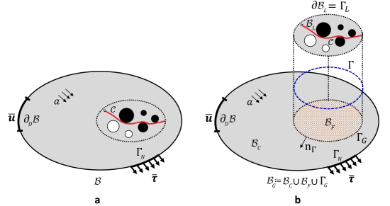
Figure 3: Illustration of the Global-Local formulation. $(a)$ Geometry and loading setup of the single-scale boundary value problem. $(b)$ Global-Local setting, by introduction of the fictitious domain ${\mathcal{B}}_{F}$ through prolongation of ${\mathcal{B}}_{C}$ to the entire domain whereas its unification is so-called global domain ${\mathcal{B}}_{G}:={\mathcal{B}}_{C}\cup\Gamma\cup{\mathcal{B}}_{F}$.

By means of the fictitious domain, the first term in Eq. 48 is recast as follows

$$\int_{{\mathcal{B}}_{C}}w(\bm{\varepsilon}(\bm{u}_{C}),1,1;{\bm{\mathnormal{M}}})\,\mathrm{d}{{\bm{\mathnormal{x}}}} =\int_{{\mathcal{B}}_{C}}w(\bm{\varepsilon}(\bm{u}_{G}),1,1;{\bm{\mathnormal{M}}})\,\mathrm{d}{{\bm{\mathnormal{x}}}}$$ (51)

$$=\int_{{\mathcal{B}}_{G}}w(\bm{\varepsilon}(\bm{u}_{G}),1,1;{\bm{\mathnormal{M}}})\,\mathrm{d}{{\bm{\mathnormal{x}}}}-\int_{{\mathcal{B}}_{F}}w(\bm{\varepsilon}(\bm{u}_{G}),1,1;{\bm{\mathnormal{M}}})\,\mathrm{d}{{\bm{\mathnormal{x}}}}.$$

Note, we substitute $\bm{u}_{G}$ for $\bm{u}_{C}$ in the second and fourth integrals in Eq. 51. That is trivial by means of the prolongation concept such that $\bm{u}_{G}|_{{\mathcal{B}}_{F}}\equiv\bm{u}_{F}$ and $\bm{u}_{G}=\bm{u}_{F}$ on $\Gamma$.

This provides the Global-Local approximation of the single-scale energy functional $\mathcal{E}$ indicated in Formulation 2.2 by

$$\widetilde{\mathcal{E}}(\bm{u}_{G},\bm{u}_{L},d_{L},\bm{u}_{\Gamma},\bm{\lambda}_{C},\bm{\lambda}_{L};{\bm{\mathnormal{M}}}): =\underbrace{\int_{{\mathcal{B}}_{G}}w({\bm{\varepsilon}}_{G},1,1;{\bm{\mathnormal{M}}})\,\mathrm{d}{{\bm{\mathnormal{x}}}}-\int_{{\mathcal{B}}_{F}}w({\bm{\varepsilon}}_{F},1,1;{\bm{\mathnormal{M}}})\,\mathrm{d}{{\bm{\mathnormal{x}}}}-\int_{\Gamma_{N,G}}{\bm{\bar{\tau}}}\cdot\bm{u}_{G}\,\mathrm{d}s}_{\text{global terms}}\,$$ (52)

$$+\underbrace{\int_{{\mathcal{B}}_{L}}w({\bm{\varepsilon}}_{L},d_{L},\nabla d_{L};{\bm{\mathnormal{M}}})\,\mathrm{d}{{\bm{\mathnormal{x}}}}}_{\text{local term}}$$

$$+\underbrace{\int_{\Gamma}\left\{\bm{\lambda}_{C}\cdot(\bm{u}_{\Gamma}-\bm{u}_{G})+\bm{\lambda}_{L}\cdot(\bm{u}_{\Gamma}-\bm{u}_{L})\right\}\mathrm{d}s}_{\text{coupling terms}}.$$

where the approximation ${\mathcal{E}}\equiv\widetilde{\mathcal{E}}$ holds.

Formulation 3.1 (Global-Local energy functional applied to the anisotropic crack topology).

Let ${\bm{\mathnormal{M}}}$, $\chi$, $\Xi$ and $\alpha$ be given with initial conditions $\bm{u}_{0}=\bm{u}(\bm{x},0)$ and $d_{0}=d(\bm{x},0)$. For the loading increments $n=1,2,\ldots,N$, find $\bm{u}_{G}:=\bm{u}_{G}^{n}\in{\bf V_{G}}$, $\bm{u}_{L}:=\bm{u}_{L}^{n}\in{\bf V_{L}}$, $\bm{u}_{\Gamma}:=\bm{u}_{\Gamma}^{n}\in{\bf H}^{1}(\Gamma)$, $d_{L}:=d_{L}^{n}\in W_{L}$, $\bm{\lambda}_{C}:=\bm{\lambda}_{C}^{n}\in{\bf L}^{2}(\Gamma)$ and $\bm{\lambda}_{L}:=\bm{\lambda}_{L}^{n}\in{\bf L}^{2}(\Gamma)$, such that the functional

$$\widetilde{\mathcal{E}}(\bm{u}_{G},\bm{u}_{L},d_{L},\bm{u}_{\Gamma},\bm{\lambda}_{C},\bm{\lambda}_{L};{\bm{\mathnormal{M}}})=$$

$$\underbrace{\int_{{\mathcal{B}}_{G}}({\frac{\lambda}{2}I^{2}_{1}+\mu I_{2}})\mathrm{d}{\textbf{x}}}_{\text{global matrix deformation term}}+\underbrace{\int_{{\mathcal{B}}_{G}}({\frac{1}{2}\chi I^{2}_{4}+2\Xi I_{5}})\mathrm{d}{\textbf{x}}}_{\text{global fiber deformtion term}}-\underbrace{\int_{\Gamma_{N,G}}{\bm{\bar{\tau}}}\cdot\bm{u}_{G}\,\mathrm{d}s}_{\text{global external load}}$$

$$-\underbrace{\int_{{\mathcal{B}}_{F}}({\frac{\lambda}{2}I^{2}_{1}+\mu I_{2}})\mathrm{d}{\textbf{x}}}_{\text{fictitious matrix deformation term}}-\underbrace{\int_{{\mathcal{B}}_{F}}({\frac{1}{2}\chi I^{2}_{4}+2\Xi I_{5}})\mathrm{d}{\textbf{x}}}_{\text{fictitious fiber deformtion term}}$$

$$+\underbrace{\int_{{\mathcal{B}}_{L}}g(d_{L+})\big{(}{\frac{\lambda}{2}I^{+2}_{1}+\mu I^{+}_{2}}\big{)}\mathrm{d}{\textbf{x}}+\int_{{\mathcal{B}}_{L}}({\frac{\lambda}{2}I^{-2}_{1}+\mu I^{-}_{2}})\mathrm{d}{\textbf{x}}}_{\text{local matrix deformation term}}+\underbrace{\int_{{\mathcal{B}}_{L}}g(d_{L+})\big{(}{\frac{1}{2}\chi I^{2}_{4}+2\Xi I_{5}}\big{)}\mathrm{d}{\textbf{x}}}_{\text{local fiber deformtion term}}$$

$$+G_{c}\underbrace{\int_{{\mathcal{B}}_{L}}\{\frac{1}{2l}(1-d_{L})^{2}+\frac{l}{2}\nabla d_{L}.\nabla d_{L}\}\mathrm{d}{\textbf{x}}}_{\text{local matrix fracture term}}+G_{c}\underbrace{\int_{{\mathcal{B}}_{L}}(\alpha\frac{l}{2}\nabla d_{L}.{\bm{\mathnormal{M}}}.\nabla d_{L})\mathrm{d}{\textbf{x}}}_{\text{local fiber fracture term}}$$

$$+\underbrace{\int_{\Gamma}\left\{\bm{\lambda}_{C}\cdot(\bm{u}_{\Gamma}-\bm{u}_{G})+\bm{\lambda}_{L}\cdot(\bm{u}_{\Gamma}-\bm{u}_{L})\right\}\mathrm{d}s}_{\text{interface coupling term}},$$

is minimized.

Note, we are not any more using $\partial_{N}{\mathcal{B}}$ for the applied surface load and hence $\Gamma_{N,G}$ is considered. This is because the global domain is free from any fracture state. The minimization problem for the Global-Local energy functional given in Formulation 3.1 that is applied to the anisotropic crack topology takes the following compact form,

$$\bm{s}=\begin{aligned} \mbox{arg}\{\mathop{\operator@font\mbox{min}}\limits_{\vbox{\halign{\ifx cc\hfil\fi\ifx rc\hfil\fi$\m@th\scriptstyle#$\ifx cc\hfil\fi\ifx lc\hfil\fi\cr\bm{u}_{G}\in{\bm{V}_{G}},\bm{u}_{L}\in{\bm{V}_{L}},\bm{u}_{\Gamma}\in{\textbf{ H}}^{1}(\Gamma),{d_{L}\in W_{L}}\;\;\crcr}}}\mathop{\operator@font\mbox{max}}\limits_{\vbox{\halign{\ifx cc\hfil\fi\ifx rc\hfil\fi$\m@th\scriptstyle#$\ifx cc\hfil\fi\ifx lc\hfil\fi\cr\bm{\lambda}_{C},\bm{\lambda}_{L}\in{\bf L}^{2}(\Gamma)\crcr}}}\,[\;\widetilde{\mathcal{E}}(\bm{u}_{G},\bm{u}_{L},d_{L},\bm{u}_{\Gamma},\bm{\lambda}_{C},\bm{\lambda}_{L};{\bm{\mathnormal{M}}})]\}\end{aligned}$$ (53)

where $\bm{s}:=(\bm{u}_{G},\bm{u}_{L},d_{L},\bm{u}_{\Gamma},\bm{\lambda}_{C},\bm{\lambda}_{L})$.

The relation between the solution $\bm{u}$ of the minimization problem in Eq. 24 and the solution triple $(\bm{u}_{G},\bm{u}_{L},\bm{u}_{\Gamma})$ of Eq. 53 reads

$$\bm{u}=\left\{\begin{tabular}[]{ll}$\bm{u}_{L},$&for ${{\bm{\mathnormal{x}}}}\in{\mathcal{B}}_{L}$,\\[2.84544pt] $\bm{u}_{G},$&for ${{\bm{\mathnormal{x}}}}\in{\mathcal{B}}_{G}$,\\[2.84544pt] $\bm{u}_{\Gamma},$&for ${{\bm{\mathnormal{x}}}}\in\Gamma$.\end{tabular}\right.$$

Remark 3.2.

When using standard single scale phase-field modeling, we are most of the time not dealing with a uniform mesh and hence the domain is divided into coarser and finer mesh elements. To resolve the crack phase-field, we need to have $l\geq h$ must hold at every point of the domain such that $l\geq h_{c}\geq h_{f}$ ($c$ and $f$ refers to the coarse and fine region in domain, respectively) satisfied. This typically leads to a finer mesh even for the area which is sufficiently far from the fracture zone, and therefore increases the computational time considerably. However, this is not the case for the Global-Local approach where the phase-field formulation is only embedded within the local domain and not the entire domain. Hence the computational time is reduced drastically.

3.3 .Variational formulation for the Global-Local coupling system

Now we consider the weak formulation of Eq. 53. The directional derivatives of the functional $\widetilde{\mathcal{E}}$ yield for the global weak form

$$\widetilde{\mathcal{E}}_{\bm{u}_{G}}(\bm{s};\delta{\bm{u}}_{G}) :=\int_{{\mathcal{B}}_{G}}\bm{\sigma}(\bm{u}_{G};{\bm{\mathnormal{M}}}):\bm{\varepsilon}(\delta{\bm{u}}_{G})\,\mathrm{d}{{\bm{\mathnormal{x}}}}-\int_{{\mathcal{B}}_{F}}\bm{\sigma}(\bm{u}_{G};{\bm{\mathnormal{M}}}):\bm{\varepsilon}(\delta{\bm{u}}_{G})\,\mathrm{d}{{\bm{\mathnormal{x}}}}$$

$$-\int_{\Gamma_{G}}\bm{\lambda}_{C}\cdot\delta{\bm{u}}_{G}\,\mathrm{d}s-\int_{\Gamma_{N,G}}{\bm{\bar{\tau}}}\cdot\delta{\bm{u}}_{G}\,\mathrm{d}s=0,$$ (G)

where $\bm{\sigma}(\bm{u}_{G}):=\partial_{\bm{\varepsilon}}w(\bm{\varepsilon}(\bm{u}_{G}),1,1;{\bm{\mathnormal{M}}})$ and $\delta{\bm{u}}_{G}\in\{{\bf H}^{1}({\mathcal{B}}_{G}):\delta{\bm{u}}_{G}=\bm{0}\;\mathrm{on}\;\partial_{D}{\mathcal{B}}\}$ is the test function. The local weak formulations assumes the form

$$\left\{\begin{tabular}[]{l}$\widetilde{\mathcal{E}}_{\bm{u}_{L}}(\bm{s};\delta{\bm{u}}_{L}):=\displaystyle\int_{{\mathcal{B}}_{L}}\bm{\sigma}(\bm{u}_{L},d_{L};{\bm{\mathnormal{M}}}):\bm{\varepsilon}(\delta{\bm{u}}_{L})\,\mathrm{d}{{\bm{\mathnormal{x}}}}-\int_{\Gamma_{L}}\bm{\lambda}_{L}\cdot\delta{\bm{u}}_{L}\,\mathrm{d}s=0$,\\[2.84544pt] $\displaystyle\widetilde{\mathcal{E}}_{d_{L}}(\bm{s};\delta d_{L}):=(1-\kappa)\int_{{\mathcal{B}}_{L}}2d_{L+}{\mathcal{H}}(\bm{\varepsilon}(\bm{u}_{L});{\bm{\mathnormal{M}}}).\delta d_{L}\mathrm{d}{{\bm{\mathnormal{x}}}}+\int_{{\mathcal{B}}_{L}}(d_{L}-1).\delta d_{L}\mathrm{d}{{\bm{\mathnormal{x}}}}$\\[2.84544pt] \qquad\qquad\; \> $\displaystyle+\int_{{\mathcal{B}}_{L}}l^{2}\nabla d_{L}.\nabla(\delta d_{L})\,\mathrm{d}{{\bm{\mathnormal{x}}}}+\int_{{\mathcal{B}}_{L}}\alpha l^{2}\nabla d_{L}.{\bm{\mathnormal{M}}}.\nabla(\delta d_{L})\,\mathrm{d}{{\bm{\mathnormal{x}}}}=0$,\\[2.84544pt] \end{tabular}\right.$$ (L)

where $\bm{\sigma}(\bm{u}_{L},d_{L};{\bm{\mathnormal{M}}})=\partial_{\bm{\varepsilon}}w({\bm{\varepsilon}}_{L},d_{L},\nabla d_{L};{\bm{\mathnormal{M}}})={{\bm{\sigma}}}_{\bm{\varepsilon}}^{iso}({\bm{\varepsilon}}_{L},d_{L})+{{\bm{\sigma}}}_{\bm{\varepsilon}}^{aniso}({\bm{\varepsilon}}_{L},d_{L},{\bm{\mathnormal{M}}})$ is defined in Eq. 22, $\delta{\bm{u}}_{L}\in{\bf H}^{1}({\mathcal{B}}_{L})$ is the local test function and $\delta d_{L}\in\text{H}^{1}({\mathcal{B}}_{L})$ is the local phase-field test function.

The variational derivatives of $\widetilde{\mathcal{E}}$ with respect to $(\bm{u}_{\Gamma},\bm{\lambda}_{C},\bm{\lambda}_{L})$ provide kinematic equations due to weak coupling between global and local form

$$\widetilde{\mathcal{E}}_{\bm{u}_{\Gamma}}(\bm{s};\delta{\bm{u}}_{\Gamma}):=\int_{\Gamma}(\bm{\lambda}_{C}+\bm{\lambda}_{L})\cdot\delta{\bm{u}}_{\Gamma}\,\mathrm{d}s=0,$$ (C₁)

$$\widetilde{\mathcal{E}}_{\bm{\lambda}_{C}}(\bm{s};\delta{\bm{\lambda}}_{C}):=\int_{\Gamma}(\bm{u}_{\Gamma}-\bm{u}_{G})\cdot\delta{\bm{\lambda}}_{C}\,\mathrm{d}s=0,$$ (C₂)

$$\widetilde{\mathcal{E}}_{\bm{\lambda}_{L}}(\bm{s};\delta{\bm{\lambda}}_{L}):=\int_{\Gamma}(\bm{u}_{\Gamma}-\bm{u}_{L})\cdot\delta{\bm{\lambda}}_{L}\,\mathrm{d}s=0.$$ (C₃)

Herein $\delta{\bm{u}}_{\Gamma}\in{\bf H}^{1}(\Gamma)$ and $\delta{\bm{\lambda}}_{C},\delta{\bm{\lambda}}_{L}\in{\bf L}^{2}(\Gamma)$ are the corresponding test functions.

Let us now focus on the global variational in (G). The presence of the two domain integrals over ${\mathcal{B}}_{G}$ and ${\mathcal{B}}_{F}$ would imply in this case the need to simultaneously access the corresponding stiffness matrices. Avoiding this can be done as follows: We focus on the domain integral over ${\mathcal{B}}_{F}$ in (G). The idea is to transform the domain integral in ${\mathcal{B}}_{F}$ to the global interface $\Gamma_{G}$. The divergence theorem leads to

$$\int_{{\mathcal{B}}_{F}}\bm{\sigma}(\bm{u}_{G}):\bm{\varepsilon}(\delta{\bm{u}}_{G})\,\mathrm{d}{{\bm{\mathnormal{x}}}}=-\int_{{\mathcal{B}}_{F}}\mathrm{div}(\bm{\sigma}(\bm{u}_{G}))\cdot\delta{\bm{u}}_{G}\,\mathrm{d}{{\bm{\mathnormal{x}}}}+\int_{\partial{\mathcal{B}}_{F}}\bm{\sigma}(\bm{u}_{G})\cdot\bm{n}_{\partial{\mathcal{B}}_{F}}\cdot\delta{\bm{u}}_{G}\,\mathrm{d}s,$$ (54)

where $\bm{n}_{\partial{\mathcal{B}}_{F}}$ is the unit outward normal vector to $\partial{\mathcal{B}}_{F}$.

The first term in the right-hand side of in Eq. 54 can be canceled by using the divergence-free assumption for the stress (no body forces in ${\mathcal{B}}_{F}$). Following a detailed argument in Gerasimov et al. [34], the second term can be further simplified

$$\int_{\partial{\mathcal{B}}_{F}}\bm{\sigma}(\bm{u}_{G})\cdot\bm{n}_{\partial{\mathcal{B}}_{F}}\cdot\delta{\bm{u}}_{G}\,\mathrm{d}s=\int_{\Gamma_{G}}\bm{\sigma}(\bm{u}_{G})\cdot\bm{n}_{\Gamma}\cdot\delta{\bm{u}}_{G}\,\mathrm{d}s+\int_{\partial{\mathcal{B}}_{F}\cap\Gamma_{N,G}}{\bm{\bar{\tau}}}\cdot\delta{\bm{u}}_{G}\,\mathrm{d}s.$$

Here, $\bm{n}_{\Gamma}:=\bm{n}_{\partial{\mathcal{B}}_{F}}$ denotes the normal vector on $\Gamma_{G}$, outward of ${\mathcal{B}}_{F}$, as illustrated in Fig. 3. Furthermore, it is possible to choose ${\mathcal{B}}_{L}$ and its coarse representation into the global level as ${\mathcal{B}}_{F}$ such that $\partial{\mathcal{B}}_{F}\cap\Gamma_{N,G}=\emptyset$. This is in line with the assumption introduced in section 3.1 that the local domain ${\mathcal{B}}_{L}$ and additionally ${\mathcal{B}}_{F}$ is free from any applied external load. Thus, the last surface integral cancels and (54) can be restated as,

$$\int_{{\mathcal{B}}_{F}}\bm{\sigma}(\bm{u}_{G}):\bm{\varepsilon}(\delta{\bm{u}}_{G})\,\mathrm{d}{{\bm{\mathnormal{x}}}}=\int_{\Gamma_{G}}\bm{\sigma}(\bm{u}_{G})\cdot\bm{n}_{\Gamma}\cdot\delta{\bm{u}}_{G}\,\mathrm{d}s,$$ (55)

such that there exists a fictitious Lagrange multiplier $\bm{\lambda}_{F}\in{\bf L}^{2}(\Gamma)$ with

$$\int_{\Gamma_{G}}\bm{\sigma}(\bm{u}_{G})\cdot\bm{n}_{\Gamma}\cdot\delta{\bm{u}}_{G}\,\mathrm{d}s=:\int_{\Gamma_{G}}\bm{\lambda}_{F}\cdot\delta{\bm{u}}_{G}\,\mathrm{d}s.$$ (56)

Here, ${\bm{\lambda}_{F}}$ is a traction-like quantity on ${\Gamma_{G}}$. Due to (55)$-$(56), the partitioned representation of equation (G) takes the following form

$$\int_{{\mathcal{B}}_{G}}\bm{\sigma}(\bm{u}_{G}):\bm{\varepsilon}(\delta{\bm{u}}_{G})\,\mathrm{d}{{\bm{\mathnormal{x}}}}-\int_{\Gamma_{G}}\bm{\lambda}_{F}\cdot\delta{\bm{u}}_{G}\,\mathrm{d}s-\int_{\Gamma_{G}}\bm{\lambda}_{C}\cdot\delta{\bm{u}}_{G}\,\mathrm{d}s-\int_{\Gamma_{N,G}}{\bm{\bar{\tau}}}\cdot\delta{\bm{u}}_{G}\,\mathrm{d}s=0,$$ (G₁)

with $\bm{\lambda}_{F}$ satisfying

$$\int_{\Gamma_{G}}\bm{\lambda}_{F}\cdot\delta{\bm{u}}_{G}\,\mathrm{d}s=\int_{{\mathcal{B}}_{F}}\bm{\sigma}(\bm{u}_{G}):\bm{\varepsilon}(\delta{\bm{u}}_{G})\,\mathrm{d}{{\bm{\mathnormal{x}}}}.$$ (G₂)

Equations (G₁), (G₂) refer to the global system of equations. The system of equations (L) is called a local variational equation and additionally (C₁), (C₂), (C₃) refer to the coupling terms. The entire system is the basis for the Global-Local approach.

3.4 .Dirichlet-Neumann type boundary conditions

To accommodate a Global-Local computational scheme, instead of finding the stationary solution of the (G₁), (G₂), (L) along with (C₁), (C₂), (C₃) in the monolithic sense, an alternate minimization is used. This is in line with [34], which leads to the Global-Local formulation through the concept of non-intrusiveness. Here the global and local level are solved in a multiplicative manner according to the idea of Schwarz’ alternating method [75].

Let $k\geq 0$ be the Global-Local iteration index at a fixed loading step $n$. The iterative solution procedure for Global-Local computational scheme is as follows:

• Dirichlet local problem: solution of local problem (L) coupled with (C₃),

• Pre-processing global level: recovery phase using (C₁) and (G₂),

• Neumann global problem: solution of global problem (G₁),

• Post-processing global level: recovery phase using (C₂).

The detailed scheme for applying the Dirichlet-Neumann type boundary conditions to the isotropic phase-field fracture modeling is described in [34].

Despite of its strong non-intrusiveness implementation point of view [32], there are two shortcomings embedded in the system which have to be resolved. (a) Due to the extreme difference in stiffness between the local domain and its projection to the global level, i.e. fictitious domain, the relaxation/acceleration techniques has to be used, see [34]. (b) Additionally, it turns out that if the solution vector $(\bm{u}_{G}^{k},\bm{u}_{L}^{k},d_{L}^{k},\bm{u}_{\Gamma}^{k},\bm{\lambda}_{C}^{k},\bm{\lambda}_{L}^{k})$ is plugged into equations (G₁), (G₂), (L), (C₁), (C₂), (C₃), the imbalanced quantities follow

$$\int_{\Gamma}(\bm{u}_{\Gamma}^{k}-\bm{u}_{L}^{k})\cdot\delta{\bm{\lambda}}_{L}\,\mathrm{d}{s}\neq 0\quad\texttt{and}\quad\int_{\Gamma}\bm{\lambda}_{F}^{k}\cdot\delta{\bm{u}}_{G}\,\mathrm{d}{s}\neq\int_{{\mathcal{B}}_{F}}\bm{\sigma}(\bm{u}_{G}^{k}):\bm{\varepsilon}(\delta{\bm{u}}_{G})\,\mathrm{d}{{\bm{\mathnormal{x}}}},$$ (57)

resulting in the iterative Global-Local computation scheme. Figure 4a depicts one iteration of the Global-Local approach by means of the Dirichlet-Neumann type boundary conditions. The aforementioned difficulties motivate us to provide an alternative coupling conditions that overcome these challenges, which are explained in the following section.

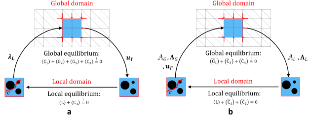
Figure 4: Global-Local iterative scheme with $(a)$ Dirichlet-Neumann type boundary conditions; $(b)$ Robin-type boundary conditions.

3.5 .Robin-type boundary conditions

In this section, the Global-Local formulation is enhanced using Robin-type boundary conditions to relax the stiff local response that is observed at the global level (due to the local non-linearity). Furthermore the computational time is reduced. This improves the resolution of the imbalanced quantities in (57) and it accelerates the Global-Local computational iterations.

Recall, the coupling equations denoted in (C₁), (C₂) and (C₃) arise from the stationary of the interface energy functional. That provides the boundary conditions which have to be imposed on the global and local levels. At that level the Robin-type boundary conditions are formulated.

• Robin-type boundary conditions at the local level

At the local level the new coupling term is introduced as a combination of (C₁) and (C₂)

$$\widetilde{\mathcal{E}}_{\bm{u}_{\Gamma}}(\bm{s};\delta{\bm{u}}_{\Gamma})+{\IKbb A}_{L}\widetilde{\mathcal{E}}_{\bm{\lambda}_{C}}(\bm{s};\delta{\bm{\lambda}}_{C})=\int_{\Gamma}(\bm{\lambda}_{C}+\bm{\lambda}_{L})\cdot\delta{\bm{u}}_{\Gamma}\,\mathrm{d}s+{\IKbb A}_{L}\int_{\Gamma}(\bm{u}_{\Gamma}-\bm{u}_{G})\cdot\delta{\bm{\lambda}}_{C}\,\mathrm{d}s=0.$$ (58)

This leads for iteration $k$ to

$$\int_{\Gamma}(\bm{\lambda}^{k-1}_{C}+\bm{\lambda}^{k}_{L})\cdot\delta{\bm{u}}_{\Gamma}\,\mathrm{d}s+{\IKbb A}_{L}\int_{\Gamma}(\bm{u}_{\Gamma}^{k,\frac{1}{2}}-\bm{u}^{k-1}_{G})\cdot\delta{\bm{\lambda}}_{C}\,\mathrm{d}s=0.$$ (59)

Herein, ${\IKbb A}_{L}$ is a local augmented stiffness matrix applied on the interface which serves as regularization of the local Jacobian matrix. By means of (59) at iteration $k$, the local system of equations results in the following boundary conditions

$$\int_{\Gamma}\bm{\lambda}^{k}_{L}\cdot\delta{\bm{u}}_{\Gamma}\,\mathrm{d}s+{\IKbb A}_{L}\int_{\Gamma}\bm{u}_{\Gamma}^{k,\frac{1}{2}}\cdot\delta{\bm{\lambda}}_{C}\,\mathrm{d}s={\bf\Lambda}^{k-1}_{L}, \widetilde{\text{C}}_{1}$$ ()

$$\int_{\Gamma}(\bm{u}_{\Gamma}^{k,\frac{1}{2}}-\bm{u}^{k}_{L})\cdot\delta{\bm{\lambda}}_{L}\,\mathrm{d}s=0, \widetilde{\text{C}}_{2}$$ ()

with

$${\bf\Lambda}^{k-1}_{L}:=\Lambda_{L}(\bm{\lambda}^{k-1}_{C},\bm{u}_{G}^{k-1};{\IKbb A}_{L})={\IKbb A}_{L}\int_{\Gamma}\bm{u}_{G}^{k-1}\cdot\delta{\bm{\lambda}}_{C}\,\mathrm{d}s-\int_{\Gamma}\bm{\lambda}^{k-1}_{C}\cdot\delta{\bm{u}}_{\Gamma}\,\mathrm{d}s.$$ (60)

Along with (L), the local system of equations has to be solved for $(\bm{u}^{k}_{L},\bm{\lambda}^{k}_{L},\bm{u}_{\Gamma}^{k,\frac{1}{2}})$ for given local Robin-type parameters $({\bf\Lambda}^{k-1}_{L},{\IKbb A}_{L})$.

• Robin-type boundary conditions at the global level

Accordingly, at the global level, the new coupling term is stated as a combination of (C₁) and (C₃)

$$\widetilde{\mathcal{E}}_{\bm{u}_{\Gamma}}(\bm{s};\delta{\bm{u}}_{\Gamma})+{\IKbb A}_{G}\widetilde{\mathcal{E}}_{\bm{\lambda}_{L}}(\bm{s};\delta{\bm{\lambda}}_{L})=\int_{\Gamma}(\bm{\lambda}_{C}+\bm{\lambda}_{L})\cdot\delta{\bm{u}}_{\Gamma}\,\mathrm{d}s+{\IKbb A}_{G}\int_{\Gamma}(\bm{u}_{\Gamma}-\bm{u}_{L})\cdot\delta{\bm{\lambda}}_{L}\,\mathrm{d}s=0.$$ (61)

This leads for iteration $k$ to

$$\int_{\Gamma}(\bm{\lambda}^{k}_{C}+\bm{\lambda}^{k}_{L})\cdot\delta{\bm{u}}_{\Gamma}\,\mathrm{d}s+{\IKbb A}_{G}\int_{\Gamma}(\bm{u}_{\Gamma}^{k}-\bm{u}^{k}_{L})\cdot\delta{\bm{\lambda}}_{L}\,\mathrm{d}s=0,$$

where, ${\IKbb A}_{G}$ is a global augmented stiffness matrix applied on the interface.

Through (61) at the iteration $k$, the Robin-type boundary condition at the global level follows

$$\int_{\Gamma}\bm{\lambda}^{k}_{C}\cdot\delta{\bm{u}}_{\Gamma}\,\mathrm{d}s+{\IKbb A}_{G}\int_{\Gamma}\bm{u}_{\Gamma}^{k}\cdot\delta{\bm{\lambda}}_{L}\,\mathrm{d}s={\bf\Lambda}^{k}_{G}, \widetilde{\text{C}}_{3}$$ ()

$$\int_{\Gamma}(\bm{u}_{\Gamma}^{k,\frac{1}{2}}-\bm{u}^{k}_{G})\cdot\delta{\bm{\lambda}}_{C}\,\mathrm{d}s=0, \widetilde{\text{C}}_{4}$$ ()

with

$${\bf\Lambda}^{k}_{G}:=\Lambda_{L}(\bm{\lambda}^{k}_{G},\bm{u}_{L}^{k};{\IKbb A}_{G})={\IKbb A}_{G}\int_{\Gamma}\bm{u}_{L}^{k}\cdot\delta{\bm{\lambda}}_{L}\,\mathrm{d}s-\int_{\Gamma}\bm{\lambda}^{k}_{L}\cdot\delta{\bm{u}}_{\Gamma}\,\mathrm{d}s.$$ (62)

Together with (G₁) and (G₂), the global system of equations has to be solved for $(\bm{u}^{k}_{G},\bm{\lambda}^{k}_{C},\bm{u}_{\Gamma}^{k})$ for a given $({\bf\Lambda}^{k}_{G},{\IKbb A}_{G},\bm{u}_{\Gamma}^{k,\frac{1}{2}})$. Here, ${\IKbb A}_{G}$ and ${\bf\Lambda}^{k}_{G}$ stand for global Robin-type parameters.

Based on the new boundary conditions provided in ($\widetilde{\text{C}}_{1}$), ($\widetilde{\text{C}}_{2}$), ($\widetilde{\text{C}}_{3}$) and ($\widetilde{\text{C}}_{4}$) the imbalanced quantities in the Global-Local iterations read

$$\int_{\Gamma}(\bm{u}_{\Gamma}^{k}-\bm{u}_{\Gamma}^{k,\frac{1}{2}})\cdot\delta{\bm{\lambda}}_{L}\,\mathrm{d}{s}\neq 0\quad\texttt{and}\quad\int_{\Gamma}\bm{\lambda}_{F}^{k}\cdot\delta{\bm{u}}_{G}\,\mathrm{d}{s}\neq\int_{{\mathcal{B}}_{F}}\bm{\sigma}(\bm{u}_{G}^{k}):\bm{\varepsilon}(\delta{\bm{u}}_{G})\,\mathrm{d}{{\bm{\mathnormal{x}}}},$$ (63)

For the specific Robin-type boundary conditions, we can resolve Eq. 63₁ such that this term does not produce any error in the iterative procedure. To do so, following Appendix B, the global and local augmented stiffness matrices within the Robin-type boundary conditions are given by

$$\framebox{$\displaystyle{\IKbb A}_{G}={\bm{L}^{T}_{L}}{\bm{T}^{-T}_{L}}{\bm{\mathcal{S}}}_{L}\quad\mbox{and}\quad{\IKbb A}_{L}:={\bm{\mathcal{S}}}_{C}.$}$$ (64)

${\IKbb A}_{G}$ and ${\IKbb A}_{L}$ can be seen as augmented stiffness matrices regularize the Jacobian stiffness matrix at the global and local levels, respectively.

Remark 3.3.

In the Robin-type boundary condition given in ($\widetilde{\text{C}}_{1}$) and ($\widetilde{\text{C}}_{3}$), we can extract different criteria, e.g.

• ${\IKbb A}_{L}\rightarrow\infty$: Dirichlet boundary conditions and ${\IKbb A}_{G}\rightarrow 0$: Neumann boundary conditions;

• ${\IKbb A}_{L}\rightarrow 0$: Neumann boundary conditions and ${\IKbb A}_{G}\rightarrow\infty$: Dirichlet boundary conditions;

• ${\IKbb A}_{L}={\bm{\mathcal{S}}}_{C}$: Robin-type boundary conditions and ${\IKbb A}_{G}\rightarrow\infty$: Dirichlet boundary conditions;

Hence, depending on the Robin-type parameters, a family of boundary conditions can be formulated.

Additionally to achieve a balance state of Eq. 63₂, the following partitioned representation of equation (G)

$$\int_{{\mathcal{B}}_{G}}\bm{\sigma}(\bm{u}_{G}):\bm{\varepsilon}(\delta{\bm{u}}_{G})\,\mathrm{d}{{\bm{\mathnormal{x}}}}-\int_{\Gamma}\bm{\lambda}_{F}\cdot\delta{\bm{u}}_{G}\,\mathrm{d}s-\int_{\Gamma}\bm{\lambda}_{C}\cdot\delta{\bm{u}}_{G}\,\mathrm{d}s-\int_{\Gamma_{N,G}}{\bm{\bar{\tau}}}\cdot\delta{\bm{u}}_{G}\,\mathrm{d}s=0, \widetilde{\text{G}}_{1}$$ ()

is equipped with a linearized $\Delta\bm{\lambda}_{F}$ satisfying

$$\int_{\Gamma}\Delta\bm{\lambda}_{F}\cdot\delta{\bm{u}}_{G}\,\mathrm{d}s=\int_{\Gamma}{\bm{\mathcal{S}}_{F}}{\Delta{{\bm{u}}}}_{G}\cdot{\delta{{\bm{u}}}}_{G}\,\mathrm{d}{{\bm{\mathnormal{x}}}}, \widetilde{\text{G}}_{2}$$ ()

where (B.6) in Appendix B is used with ${{{\bm{u}}}_{F}}={{{\bm{u}}}_{G}}$. Note that now the second imbalance quantity shown in (63) does not anymore produce an error. We are not solving for $\bm{\lambda}_{F}$ and in the linearized equation of ($\widetilde{\text{G}}_{1}$) this term is replaced by ($\widetilde{\text{G}}_{2}$). The linearized equation of ($\widetilde{\text{G}}_{1}$) is solved within a single iteration, because we are dealing with a linear elastic constitutive equations.

The detailed Global-Local formulation using Robin-type boundary conditions is depicted in Algorithm 1. Accordingly, Fig. 4b depicts one iteration of the Global-Local coupling scheme by means of the Robin-type boundary conditions. The Global-Local setting provides a generic two-scale finite element algorithms that enables capturing local non-linearities.

3.6 .Spatial discretization

The computational domain is subdivided into bilinear quadrilateral elements denoted as ${Q}_{1}$. Both subproblems are discretized with a Galerkin finite element method using $H^{1}$-conforming bilinear (2D) elements, i.e., the ansatz and test space uses $Q_{1}^{c}$–finite elements, e.g., for details, we refer readers to the [21]. Consequently, the discrete spaces have the property $V_{h}\subset V$ and $W_{h}\subset W$. Here, $h$ refers to the finite element size. Accordingly, a finite element discretization is illustrated in Appendix A for the primal fields refers to the $(\bm{u}_{G},\bm{u}_{L},d_{L},\bm{u}_{\Gamma},\bm{\lambda}_{C},\bm{\lambda}_{L})$ and its constitutive state variables represented by $({\bm{\varepsilon}}_{G},{\bm{\varepsilon}}_{L},d_{L},\nabla d_{L})$.

Algorithm 1 Global-Local iterative scheme combined with Robin-type boundary conditions.

Input: loading data $(\bar{\bm{u}}_{n},\bar{\bm{\tau}}_{n})$ on $\partial_{D}{\mathcal{B}}$ and $\Gamma_{N}$, respectively;

solution $(\bm{u}_{G,n-1},\bm{u}_{L,n-1},d_{L,n-1},\bm{u}_{\Gamma,n-1},\bm{\lambda}_{C,n-1},\bm{\lambda}_{L,n-1})$ and ${\mathcal{H}}_{L,n-1}$ from step $n-1$.

Global-Local iteration $k\geq 1$:

Local boundary value problem:

•  given ${\IKbb A}_{L},{\bf\Lambda}^{k-1}_{L},{\mathcal{H}}_{L,n-1}$; solve

phase-field part:

$\displaystyle(1-\kappa)\int_{{\mathcal{B}}_{L}}d_{L+}{\mathcal{H}}(\bm{\varepsilon}(\bm{u}_{L})).\delta d_{L}\mathrm{d}{\bm{x}}+G_{c}\int_{{\mathcal{B}}_{L}}\frac{1}{l}(d_{L}-1).\delta d_{L}\mathrm{d}{\bm{x}}$

$\displaystyle+G_{c}\int_{{\mathcal{B}}_{L}}l\nabla d_{L}.\nabla(\delta d_{L})\mathrm{d}{\bm{x}}+G_{c}\int_{{\mathcal{B}}_{L}}\alpha l\nabla d_{L}.{\bm{\mathnormal{M}}}.\nabla(\delta d_{L})\mathrm{d}{\bm{x}}=0$,

mechanical part:

$\left\{\,\vbox{\halign{\strut@$\m@th\displaystyle#$\hfil&\quad\strut@{#}\hfil\cr\hbox{\vrule height=0.0pt,depth=0.0pt,width=0.0pt}$\displaystyle\displaystyle\int_{\Omega_{L}}\bm{\sigma}(\bm{u}_{L},d_{L}):\bm{\varepsilon}(\delta{\bm{u}}_{L})\,\mathrm{d}{{\bm{\mathnormal{x}}}}-\int_{\Gamma}\bm{\lambda}_{L}\cdot\delta{\bm{u}}_{L}\,\mathrm{d}{s}=0,\\\displaystyle\int_{\Gamma}\bm{\lambda}_{L}\cdot\delta{\bm{u}}_{\Gamma}\,\mathrm{d}s+{\IKbb A}_{L}\int_{\Gamma}\bm{u}_{\Gamma}\cdot\delta{\bm{\lambda}}_{C}\,\mathrm{d}s={\bf\Lambda}^{k-1}_{L},\\\displaystyle\int_{\Gamma}(\bm{u}_{\Gamma}-\bm{u}_{L})\cdot\delta{\bm{\lambda}}_{L}\,\mathrm{d}s=0,\crcr}}\right.$      •   set $(\bm{u}_{L},d_{L},\bm{u}_{\Gamma},\bm{\lambda}_{L})=:(\bm{u}_{L}^{k},d_{L}^{k},\bm{u}_{\Gamma}^{k,\frac{1}{2}},\bm{\lambda}_{L}^{k})$,     •  given $({\bm{u}_{L}^{k}},{\bm{\lambda}^{k}_{L}};{\IKbb A}_{G})$, set                            $\displaystyle{\bf\Lambda}^{k}_{G}={\IKbb A}_{G}\int_{\Gamma}\bm{u}_{L}^{k}\cdot\delta{\bm{\lambda}}_{C}\,\mathrm{d}s-\int_{\Gamma}\bm{\lambda}^{k}_{L}\cdot\delta{\bm{u}}_{\Gamma}\,\mathrm{d}s$. [0.5cm]   Global boundary value problem:       •  given ${\IKbb A}_{G},{\bf\Lambda}^{k}_{G},\bm{u}_{\Gamma}^{k,\frac{1}{2}}$, solve                         $\left\{\,\vbox{\halign{\strut@$\m@th\displaystyle#$\hfil&\quad\strut@{#}\hfil\cr\hbox{\vrule height=0.0pt,depth=0.0pt,width=0.0pt}$\displaystyle\displaystyle\int_{\Omega_{G}}\bm{\sigma}(\bm{u}_{G}):\bm{\varepsilon}(\delta{\bm{u}}_{G})\,\mathrm{d}{{\bm{\mathnormal{x}}}}-\int_{\Gamma}\bm{\lambda}_{F}\cdot\delta{\bm{u}}_{G}\,\mathrm{d}{s}-\int_{\Gamma}\bm{\lambda}_{C}\cdot\delta{\bm{u}}_{G}\,\mathrm{d}{s}-\int_{\Gamma_{N}}\bar{\bm{\tau}}\cdot\delta{\bm{u}}_{G}\,\mathrm{d}{s}=0,\\\displaystyle\int_{\Gamma}\bm{\lambda}_{C}\cdot\delta{\bm{u}}_{\Gamma}\,\mathrm{d}s+{\IKbb A}_{G}\int_{\Gamma}\bm{u}_{\Gamma}\cdot\delta{\bm{\lambda}}_{C}\,\mathrm{d}s={\bf\Lambda}^{k}_{G},\\\displaystyle\int_{\Gamma}(\bm{u}_{\Gamma}^{k,\frac{1}{2}}-\bm{u}_{G})\cdot\delta{\bm{\lambda}}_{C}\,\mathrm{d}s=0,\crcr}}\right.$       •  set $(\bm{u}_{G},\bm{u}_{\Gamma},\bm{\lambda}_{C})=:(\bm{u}_{G}^{k},\bm{u}_{\Gamma}^{k},\bm{\lambda}_{C}^{k})$,     •  given $({\bm{u}_{G}^{k}},{\bm{\lambda}^{k}_{C}};{\IKbb A}_{L})$, set                            $\displaystyle{\bf\Lambda}^{k}_{L}={\IKbb A}_{L}\int_{\Gamma}\bm{u}_{G}^{k}\cdot\delta{\bm{\lambda}}_{C}\,\mathrm{d}s-\int_{\Gamma}\bm{\lambda}^{k}_{C}\cdot\delta{\bm{u}}_{\Gamma}\,\mathrm{d}s$.       •  if fulfilled, set $(\bm{u}_{G}^{k},\bm{u}_{L}^{k},d_{L}^{k},\bm{u}_{\Gamma}^{k},\bm{\lambda}_{C}^{k},\bm{\lambda}_{L}^{k})=:(\bm{u}_{G,n},\bm{u}_{L,n},d_{L,n},\bm{u}_{\Gamma,n},\bm{\lambda}_{C,n},\bm{\lambda}_{L,n})$ and stop;       •  else $k+1\rightarrow k$. [0.5cm] Output: solution $(\bm{u}_{G,n},\bm{u}_{L,n},d_{L,n},\bm{u}_{\Gamma,n},\bm{\lambda}_{C,n},\bm{\lambda}_{L,n})$ and ${\mathcal{H}}_{L,n}$.

4 .Predictor-Corrector Adaptivity Applied to the Global-Local Formulation

We assume the Global-Local formulation is at the converged state, which is denoted as $(\bm{u}_{G,n},\bm{u}_{L,n},d_{L,n}$ $,\bm{u}_{\Gamma,n},\bm{\lambda}_{C,n},\bm{\lambda}_{L,n})$. The Global-Local approach is augmented by a dynamic allocation of a local state using an adaptive scheme which has to be performed at time step $t_{n}$. By the adaptivity procedure, we mean: (a) to determine which global elements need to be refined and identified by ${\mathcal{B}}^{\;adapt}_{G}\subset{\mathcal{B}}_{G}$; (b) to create the new fictitious domain ${\mathcal{B}}^{\;new}_{F}:={\mathcal{B}}^{\;old}_{F}\cup{\mathcal{B}}^{\;adapt}_{F}$ with ${\mathcal{B}}^{\;adapt}_{F}:={\mathcal{B}}^{\;adapt}_{G}$ and as a result a new local domain is defined as ${\mathcal{B}}^{\;new}_{L}:={\mathcal{B}}^{\;old}_{L}\cup{\mathcal{B}}^{\;adapt}_{L}$, see Fig. 5; (c) to determine a new local interface denoted as $\Gamma_{L}$; (d) to interpolate the old global solution in ${\mathcal{B}}^{\;adapt}_{L}$. All these steps refer to predictor steps. The corrector step is explained in Section 4.2. We briefly notice that the principal idea of this adaptive scheme is inspired from [42] in which a predictor-corrector scheme for mesh refinement in the crack zone was proposed.

4.1 .Predictor step

In this section, we start explaining the predictor step.

• Determining global elements which have to be refined

Recall that the interfaces at the global, fictitious and local domains are denoted by $\Gamma_{G}\subset{\mathcal{B}}_{G}$, $\Gamma_{F}\subset{\mathcal{B}}_{F}$ and $\Gamma_{L}\subset{\mathcal{B}}_{L}$. We denote $e_{G}\in{\mathcal{B}}_{G}$, $e_{F}\in{\mathcal{B}}_{F}$ and $e_{L}\in{\mathcal{B}}_{L}$ as the elements in the global, fictitious and local domain. Let $E^{1}_{G,i},E^{2}_{G,i},E^{3}_{G,i}$ and $E^{4}_{G,i}$ refer to the left, top, right and bottom global edges for the $i^{th}$ element $e_{G,i}$, respectively (because, it is quadrilateral hence it has four edges). Accordingly, $E^{q}_{F,i}\in e_{F,i}$ and $E^{q}_{L,i}\in e_{L,i}$ with $\;q=(1,2,3,4)$ refer to the fictitious and local edges, see Fig. 5.

We now develop a procedure, to determine the global elements $e_{G,i}$ which have at least one edge $E^{q}_{G,i}$ such that their fine resolution at the local level, i.e. $E^{q}_{L,i}$, reaches to the crack phase-field threshold value. Thus $e_{G,i}$ has to be refined. The predictor step for the adaptive scheme of the Global-Local formulation is explained in Algorithm 2.

Algorithm 2 Predictor step for the adaptive procedure.

Let $0<\texttt{TOL}_{d}<1$ be given. For the $d_{L}:=d_{L,n}\;\in{\mathcal{B}}_{L}$, find corresponding $e_{G}\in{\mathcal{B}}_{G}$ which must be refined using the following steps:

1. Find $\bm{x}_{L}\in\Gamma_{L}$ such that $d_{L}({\bm{x}}_{L})<\texttt{TOL}_{d}$ on $\Gamma_{L}$:[2mm] Checking criterion: If ”Yes” proceed to step 2. If ”No” stop,

2. find $E^{q}_{L,i}\in\Gamma_{L}$ such that ${\bm{x}_{L}}\in E^{q}_{L,i}$,

3. find $E^{q}_{G,i}={\mathcal{P}}^{-1}E^{q}_{L,i}$ (corresponding edge in ${\mathcal{B}}_{G}$),

4. find $e_{G}\in{\mathcal{B}}_{G}$ and $e_{G}\not\in{\mathcal{B}}_{F}$ such that $E^{q}_{G,i}\in e_{G}$.

Here, ${\mathcal{P}}:\Gamma_{G}\rightarrow\Gamma_{L}$ is denoted as a projection/geometrical operator which maps the global to the local interface by $E^{q}_{L,i}:={\mathcal{P}}E^{q}_{G,i}$.

• Creating new fictitious and local domains: $({\mathcal{B}}^{\;new}_{F},{\mathcal{B}}^{\;new}_{L})$

We are now able to determine a new fictitious and local domains. Knowing $e_{G}$ from the previous step, the new fictitious domain is ${\mathcal{B}}^{\;new}_{F}:={\mathcal{B}}^{\;old}_{F}\cup{\mathcal{B}}^{\;adapt}_{F}$ such that ${\mathcal{B}}^{\;adapt}_{F}:=e_{G}$. As a result, a new local domain is ${\mathcal{B}}^{\;new}_{L}:={\mathcal{B}}^{\;old}_{L}\cup{\mathcal{B}}^{\;adapt}_{L}$ such that ${\mathcal{B}}^{\;adapt}_{L}$ is a fine discretization (including heterogeneity as well) of ${\mathcal{B}}^{\;adapt}_{F}$, see Fig. 5.

• Determining the coupling interface: $(\Gamma_{G},\;\Gamma_{F},\;\Gamma_{L})$

So far, we have identified new fictitious and local domains. Next, we determine $\Gamma_{F}\subset{\mathcal{B}}_{F}$, due to its coarse discretization. Afterwards, we find the local interface $\Gamma_{L}\subset{\mathcal{B}}_{L}$ by projecting $\Gamma_{F}$ to ${\mathcal{B}}_{L}$. Finally, it is trivial that $\Gamma_{G}:=\Gamma_{F}$, because ${\mathcal{B}}_{F}$ and ${\mathcal{B}}_{G}$ are in the same discretization space.

The edge $E^{q}_{F,i}\in\Gamma_{F}$ is on the interface if

$$E^{q}_{F,i}\in\Gamma_{F}\;\;\mbox{if}\;\;\nexists\;\;i,j\;:E^{q}_{F,i}=E^{r}_{F,j},\quad\mbox{for}\;q,r=(1,2,3,4),$$ (65)

which means if an edge $E^{q}_{F,i}$ is shared between two elements in ${\mathcal{B}}_{F}$, it is not on the interface (inner edge) and if it belongs only to one element, then it must also belong to interface (outer edge). As a result, we define the fictitious interface as $\Gamma_{F}=\mathop{\operator@font{\huge\texttt{A}}}\limits_{\vbox{\halign{\ifx cc\hfil\fi\ifx rc\hfil\fi$\m@th\scriptstyle#$\ifx cc\hfil\fi\ifx lc\hfil\fi\cr i,q\crcr}}}\,E^{q}_{F,i}$, hence $\Gamma_{L}=\mathop{\operator@font{\huge\texttt{A}}}\limits_{\vbox{\halign{\ifx cc\hfil\fi\ifx rc\hfil\fi$\m@th\scriptstyle#$\ifx cc\hfil\fi\ifx lc\hfil\fi\cr i,k\crcr}}}\,E^{q}_{L,i}$ with $E^{q}_{L,i}:={\mathcal{P}}E^{q}_{F,i}$.

• Interpolating the old solution at $t^{n}$ from the global to the local mesh

Given a continuous function $\bm{u}^{adapt}_{G}$ that is $\bm{u}_{G}$ in ${\mathcal{B}}^{\;adapt}_{G}$, we define the linear interpolation operator $\mathcal{\pi}:{\mathcal{B}}^{\;adapt}_{G}\rightarrow{\mathcal{B}}^{\;adapt}_{L}$ to $\bm{u}^{adapt}_{G}$ by

$${\bm{u}^{adapt}_{L,n}}(\bm{x}):=\mathcal{\pi}{\bm{u}^{adapt}_{G,n}}=\bm{N}_{u}^{G}(\bm{x}){\hat{\bm{u}}^{adapt}_{G,n}}\quad\mbox{for}\;\;{\bm{x}}\in{\mathcal{B}}^{\;adapt}_{L}.$$ (66)

where $\bm{N}_{u}^{G}(x)$ is defined in Appendix A. Hence, ${\bm{u}^{new}_{L,n}}:={\bm{u}_{L,n}}\cup{\bm{u}^{adapt}_{L,n}}$.

4.2 .Corrector step

We introduce a corrector step in which the computation is rerun on the newly determined local mesh. To this end, we compute Global-Local solutions until the checking criterion in Algorithm 2 is not satisfied (No). That means we could not find additional local edges on the interface such that $d_{L}({\bm{x}}_{L})<\texttt{TOL}_{d}$ on $\Gamma_{L}$ holds.

Let us write Algorithm 1 in the following abstract form

$${\bm{s}_{n}}=\texttt{GL}({\bm{s}_{n-1}}),$$ (67)

with ${\bm{s}}=(\bm{u}_{G},\bm{u}_{L},d_{L},\bm{u}_{\Gamma},\bm{\lambda}_{C},\bm{\lambda}_{L})$. We define an intermediate solution ${\bm{s}^{j}_{n-1}}$ at fixed $t^{n}$ such that the corrector step for adaptive scheme reads,

$${\bm{s}^{j}_{n-1}}=\texttt{GL}({\bm{s}_{n-1}}).$$ (68)

Perform Algorithm 2, if the checking criterion in step 1 is satisfied. But, if this is not the case, then the corrector step is fulfilled, thus set ${\bm{s}^{j}_{n-1}}=:{\bm{s}_{n}}$ and stop; else $j+1\rightarrow j$.

4.3 .The final predictor-corrector scheme

The aforementioned predictor-corrector adaptivity procedure is summarized in Algorithm 3 as follows,

Algorithm 3 Predictor-corrector steps for the adaptive procedure.

Let $0<\texttt{TOL}_{d}<1$ be given. For the $d_{L}:=d_{L,n}\;\in{\mathcal{B}}_{L}$, find corresponding $e_{G}\in{\mathcal{B}}_{G}$ which have to be refined using the following steps:

1. Compute the intermediate solution by ${\bm{s}^{j}_{n-1}}=\texttt{GL}({\bm{s}_{n-1}})$,

2. perform Algorithm 2 if Checking criterion is satisfied (Yes),

3. if checking criterion in Algorithm 2 is not satisfied, then the corrector step is fulfilled, thus set ${\bm{s}^{j}_{n-1}}=:{\bm{s}_{n}}$ and stop; else $j+1\rightarrow j$.

Fig. 5 depicts one iteration of the predictor-corrector steps for the adaptive procedure which is illustrated in Algorithm 3.

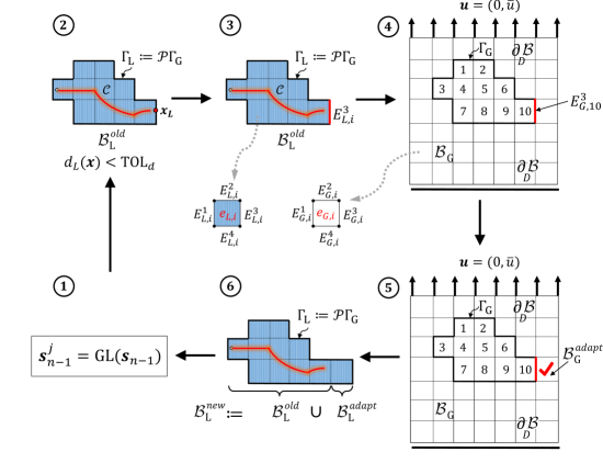
Figure 5: Explanation of the predictor-corrector adaptive scheme.

We notice that for the brutal fracture behavior, where a complete failure happens in one load increment, Algorithm 3 has an important effect. This is mainly because the corrector step is performed until there is no nodal point on the interface such that $d_{L}({\bm{x}}_{L})<\texttt{TOL}_{d}$ holds. If this is fulfilled, the adaptivity procedure stops and goes to the next load increment. Thus brutal fracture can be observed in the next time step. This is illustrated in the numerical example of the Section 5.4.2.

The performance of Algorithm 2 and Algorithm 3 is depicted in Fig. 6 and Fig. 7. This example refers to the isotropic single-edge notch under tension. The numerical setup is given in [67]. By applying predictor-corrector steps, we will have a more regularized fracture surface. This is observed for instance in Fig. 7 step 58, step 60 and step 62 (right figures). But that is not the case, if we only apply predictor step. For instance in Fig. 6, at step 58, after the predictor step (in the absence of the corrector stage). Here we do not have a regularized fracture surface. It will be regularized in the next load increment which is shown in step 59 . That is also observed in steps 60 and 63 in Fig. 6, as well. To compare these effects on the global level, we refer to the load-displacement curve in Fig. 10a. It was observed that the corrector procedure applied to the predictor step improved the Global-Local results.

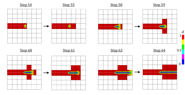
Figure 6: Global-Local approach augmented with the predictor adaptive scheme given in Algorithm 2; Fracture of isotropic single-edge-notched plate under tension per loading steps.

Figure 7: Global-Local approach augmented with the predictor-corrector adaptive scheme indicated in Algorithm 3; Fracture of isotropic single-edge-notched plate under tension per loading steps.

4.4 .Homogenized phase-field solution on the global level

We determine the coarse representation of the crack phase-field. Here we denote $(\bm{u}_{G,n},\bm{u}_{L,n},d_{L,n}$ $,\bm{u}_{\Gamma,n},\bm{\lambda}_{C,n},\bm{\lambda}_{L,n})$ to be the converged solution of the Global-Local approach. We emphasis that the computation of the global phase-field $d_{G}$ is a post-processing step. The homogenized global crack phase-field solution can be determine based on the following ways.

(a) Global crack phase-field solution. We solve the crack phase-field given in (29) after having obtained the converged global solution by

$$d_{G}=\mathop{\operator@font\mbox{argmin}}\limits_{\vbox{\halign{\ifx cc\hfil\fi\ifx rc\hfil\fi$\m@th\scriptstyle#$\ifx cc\hfil\fi\ifx lc\hfil\fi\cr d_{G}\in W\crcr}}}\,[-g^{\prime}({d_{G+}){\mathcal{H}}(\bm{u}_{G,n};{\bm{\mathnormal{M}}}_{G})-l_{G}\delta_{d}.\gamma_{l}}],$$ (69)

with,

$$l_{G}:=l_{L}\frac{h_{G}}{h_{L}}\quad\mbox{and}\quad{\bm{\mathnormal{M}}}_{G}:={\bm{\mathnormal{M}}}_{L}.$$ (70)

where ${\mathcal{H}}$ is described by (34) and formulated on the global level. The last condition in (70)₂ holds because we assumed the structural tensor at the global level inclined with identical angle as the local level. This holds in the case of the transverse isotropic setting.

(b) Homogeneous crack phase-field solution. Assume that at the global level the transition zone of the crack phase-field vanishes. That results in a free isotropic and anisotropic Laplacian operator $\Delta(\bullet)=0$ in (29). Hence, the second and third terms in (36) become zero. Following that Eq. 29 at the quasi-static stationery state is restated by

$$d_{G}=\frac{1}{1+2(1-\kappa){\mathcal{H}}(\bm{u}_{G,n};{\bm{\mathnormal{M}}}_{G})}\;\in[0,1],$$ (71)

such that if ${\mathcal{H}}\rightarrow\infty\;\mbox{then}\;d_{G}=0$ and for ${\mathcal{H}}\rightarrow 0\;\mbox{then}\;d_{G}=1$ holds. The homogeneous crack phase-field solution $d_{G}$ in (71) is independent of the $l_{G}$ but the global crack phase-field solution in (69) depends on $l_{G}$. At the global level we do not have any given imperfection (e.g. notch shaped). That is located only at the local level. However, (69) or (71) still provides the desired crack direction because of ${\mathcal{H}}(\bm{u}_{G,n};{\bm{\mathnormal{M}}}_{G})$. This is due to the fact that $\bm{u}_{G,n}$ is determined based on the given $\bm{u}_{\Gamma}^{k,\frac{1}{2}}$ which is upscaled from local level, see ($\widetilde{\text{C}}_{4}$). As a result, the crack driving force at the global level is the true projection of the constitutive non-linearity at the local level. That is varitionally consistent and resulting from the upscaling procedure (i.e. information which is transformed from the local level to the global scale).

5 .Numerical Examples

The section presents the performance of the proposed adaptive Global-Local approach applied to the phase-field modeling of anisotropic brittle fracture. We consider four numerical model problems. The first example deals with an isotropic single-edge-notched shear test in which we set the directional tensor to be zero. The next three examples deal with transverse isotropic setting with different directional tensors.

5.1 .Goals of the computations

For comparison purposes, we compute quantitative and qualitative single scale and Global-Local resolutions. In detail, we investigate:

• Crack patterns on the local scale at the complete fracture state in order to evaluate the down-scaling procedure (i.e. transition of external loading increments from the global scale to the local level);

• Load-displacement curves to evaluate the up-scaling procedure during the Global-Local coupling approach (i.e. transition of local non-linearity and heterogeneity responses to the global level);

• Investigations of the thermodynamically consistency between the single scale strain-energy and its Global-Local energy functional;

• Efficiency of the overall response resulting from the predictor-corrector adaptive scheme;

• Effect of the given threshold phase-field value in the adaptive process for the derivation of the fracture zone;

• Evaluating the homogenized phase-field solution at the global level, when the Global-Local scheme is in the converged state.

The outlined constitutive formulation is considered to be a canonically consistent and robust scheme for capturing the non-linearities on the lower level and its projection on to the global level.

5.2 .Geometry, data and solution procedures

As a setup for the numerical investigations, we use:

• Geometries and parameters: In the first two examples, a boundary value problem applied to the square plate is shown in Fig. 8. We set $A=0.5\;mm$ hence ${\mathcal{B}}=(0,1)^{2}$ $mm^{2}$ that includes a predefined single notch from the left edge to the body center, as depicted in Fig. 8. The predefined crack is in the $y=A$ plane and is restricted in $0\leq|\mathcal{C}|\leq l_{0}$ and we set $l_{0}=A=0.5$. As a loading setup, we set the initial values for displacement and phase-field as $\bm{u}_{0}:=0\in{\mathcal{B}}$ and $d_{0}:=1\in{\mathcal{B}}_{C}$ and ${\mathcal{B}}_{L}$. The finite element discretization is explained in Section 3.6. Details of the last two examples are accordingly given.

• Material parameters: In the first two examples, the constitutive parameters for the isotropic and transversely isotropic material are the same as in [68] and given as $\lambda=121.15$ kN/mm², $\mu=80.77$ kN/mm². Griffith’s critical elastic energy release rate is set as $G_{c}=2.7\times 10^{-3}$ kN/mm. In the first example, the preferred fiber direction is set to zero ${\bm{a}}=0$ which represents the standard isotropic setting. Whereas, the three other examples represent transversely isotropic behavior that is characterized by the symmetric second-order structural tensor ${\bm{\mathnormal{M}}}={\bm{a}}\otimes{\bm{a}}$. For a given angle $\phi$ of the preferred fiber direction, the normal vector is defined as ${\bm{a}}:=~{}\big{[}cos(\phi)\quad sin(\phi)\big{]}^{T}$. For the second example, the preferred fiber direction is given by the structural director ${\bm{\mathnormal{a}}}$ which is inclined by $\theta=+30^{\circ}$ and $\theta=-30^{\circ}$ with respect to the $x$-axis of a fixed Cartesian coordinate system in the Sections 5.4.1 and 5.4.2, respectively. Additionally, the anisotropy penalty-like parameters for the deformation part and fracture contribution are set to $\alpha=\chi=50$ and $\Xi=0$. All material properties are fixed for the following numerical examples, unless indicated otherwise.

• Model parameters: The phase-field parameters are chosen as $\kappa=10^{-10}$ and $l=2h$. The threshold value for the Global-Local predictor-corrector mesh refinement scheme is $\texttt{TOL}_{d}=0.85$. This threshold value $\texttt{TOL}_{d}$ is a fixed value except for the compression cases in which we use a different $\texttt{TOL}_{d}$.

• Solution of the nonlinear problems:

  An alternate minimzation scheme is used for solving the local boundary value problem indicated in Algorithm 1. Thus, we alternately solve for $d_{L}$ by fixing ${\bm{u}}_{L}$ and then solving for $({\bm{u}}_{L},{\bm{u}}_{\Gamma},{\bm{\lambda}_{L}})$ by fixing $d_{L}$ until convergence is reached. An iterative Newton solver is used in which the linear equation systems are solved with a generalized minimal residual method. The stopping criterion of the single scale and local Newton methods is $\texttt{Tol}_{\texttt{N-R}}=10^{-10}$. Specifically, the relative residual norm is given by $\texttt{Residual}:\|\bm{F}(\bm{x}_{k+1})\|\leq\texttt{Tol}_{\texttt{N-R}}\|\bm{F}(\bm{x}_{k})\|$. Here, $\bm{F}$ refers to the residual of the equilibrium equation of the nonlinear single scale and local boundary value problems.

• Software:

  The implementation is based on MATLAB R2018b [63] and Fortran 90 [19]. The user elements including the constitutive modeling at each Gaussian quadrature points are written in Fortran 90. The general framework for the Global-Local approach is implemented in MATLAB as a parent/main program such that all subprograms in Fortran 90 are called as a Mex-file.

Figure 8: Geometry and loading setup for the single-edge-notched shear test in (a) and tensile test with the structural director $\bm{a}$ inclined under an angle $\phi=+30$ in (b) and $\phi=-30$ in (c) with respect to the $x$-axis.

5.3 .Example 1: Isotropic single-edge-notched shear test

In this example, attention is restricted to pure isotropic crack-propagation by letting ${\bm{a}}=0$. In this setting, we consider a shear test such that fracture response exhibits a curved surface. The numerical computation is performed by applying a monotonic displacement $\bar{{\bm{\mathnormal{u}}}}=5\times 10^{-5}$ in horizontal direction at the top boundary of the specimen.

An important aspect that has to be verified at the local level is the fracture state. Thus, we look at the crack phase field pattern at the local scale to investigate the transition of external loading increments (i.e. the down-scaling procedure) from the global domain to the local level. The Global-Local adaptive scheme to capture the curved surface is evaluated for different $\texttt{TOL}_{d}$. Hereby, $\texttt{TOL}_{d}$ leads to different fracture zones and hence different local domains. Four different values of $\texttt{TOL}_{d}:=(0.9,0.85,0.80,0.70)$ are considered. Fig. 9 shows the evolution of the local domains for different $\texttt{TOL}_{d}$. The global mesh is only used to show a clear representation for the evolution of the local domain. Since global and local domains are performed independently, and therefore we deal with a two-scale finite element algorithm.

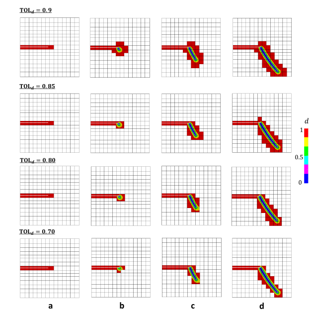
Figure 9: Example 1. Evolution of the local domain for different threshold values of $\texttt{TOL}_{d}$ and four deformation states up to final failure, (a) $\bar{\bm{u}}=0.0058\;mm$ (b) $\bar{\bm{u}}=0.0103\;mm$ (c) $\bar{\bm{u}}=0.0117\;mm$ (d) $\bar{\bm{u}}=0.0180\;mm$.

By comparing e.g. the first and fourth row in Fig. 9, it is trivial that a smaller value of the $\texttt{TOL}_{d}$ yields a narrow fracture zone. Hence, if $\texttt{TOL}_{d_{1}}<\texttt{TOL}_{d_{2}}$ then $|{\mathcal{B}}_{L,1}|<|{\mathcal{B}}_{L,2}|$. The resultant narrow local domain due to the adaptivity approach in Fig. 9 demonstrates the great efficiency of the proposed method.

The above observation plays an important role by constraining the diffusivity zone of the crack phase-field in a narrow fracture region. Whereas in the standard single scale phase field modeling, the fracture zone is spread over more areas and hence a wider diffusive zone. Thus, by the Global-Local approach we limit the effect of diffusivity on the local level and not in the entire domain.

The influence of local effects (non-linear constitutive responses) on the global scale are described based on the load-displacement response, depicted in Fig. 10b.

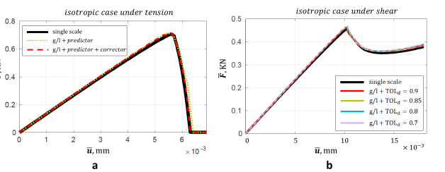
Figure 10: Load-displacement curves for the isotropic single-edge-notched test, (a) Example in Section 4, specimen under tension test and (b) Example 1, shear test based on Global-Local approach with different $\texttt{TOL}_{d}$ verses single scale.

These curves are in a good agreement with the single scale solution. As it is excepted the Global-Local approach with a higher value of the $\texttt{TOL}_{d}=0.90$ is in very good agreement with the single scale solution. That is mainly because within single scale phase-field modeling, we deal with a wider diffusivity zone and hence more elements with fracture state are involved.

The use of adaptivity leads to a narrow fracture zone and hence to a reduction of degrees of freedom. That is shown in Fig. 11a for different values of $\texttt{TOL}_{d}$. It turns out that a smaller values of $\texttt{TOL}_{d}$ lead to a reduction of the active degrees of freedom and the computational time. At every jump which appears in Fig. 11a the predictor-corrector adaptive scheme is applied to the Global-Local scheme hence the number of degrees of freedom is increased.

More specifically, we show that the adaptive scheme applied to the Global-Local approach considerably reduces the computational cost in comparison with the single scale solution, as indicated in Fig. 11b. Note that, at load step $\bar{\bm{u}}=10\times 10^{-3}$ (the loading point where the fracture initiates) a higher computational time is observed, see Fig. 11. That is due to the alternate minimization approach used for solving the variational phase-field formulation which needs more iteration at cracking to reach the equilibrium state.

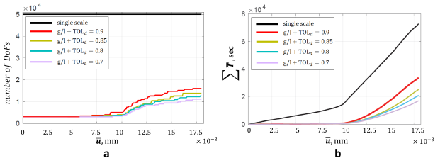
Figure 11: Example 1. Isotropic single-edge-notched shear test. (a) Number of degrees of freedom which have to solved for and (b) Time-displacement curves in terms of the accumulated time.

We now aim to investigate the energy response when solving a problem as single scale problem and as Global-Local. Recall, the consistency of the energy functional (departing point of the Global-Local approximation)

$${\mathcal{E}}(\bm{u},d;{\bm{\mathnormal{M}}})\equiv\widetilde{\mathcal{E}}(\bm{u}_{G},\bm{u}_{L},d_{L},\bm{u}_{\Gamma},\bm{\lambda}_{C},\bm{\lambda}_{L};{\bm{\mathnormal{M}}}),$$

between the single scale and the Global-Local functional indicated in Formulation 2.2 and (52), respectively. We investigate this approximation by means of the evolution of the total stored elastic strain energy plotted in Fig. 12a and the dissipated fracture energy shown in Fig. 12b during load increments. These Global-Local simulation results show very good agreement with the single scale scheme yet with its efficiency in time shown in Fig. 11b.

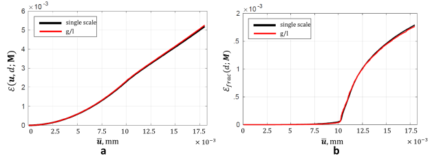
Figure 12: Example 1. Comparison of the energy response between the single scale domain and the Global-Local scheme for (a) the total free-energy functional and (b) the dissipated fracture energy.

At the converged Global-Local state, we obtain the following updated fields: $(\bm{u}_{G,n},\bm{u}_{L,n}$ $,d_{L,n},\bm{u}_{\Gamma,n},\bm{\lambda}_{C,n},\bm{\lambda}_{L,n})$. Based on that, the homogenized global phase-field solution at the complete failure state is illustrated in Fig. 13 for different values of $\texttt{TOL}_{d}$. We emphasis that in the global level there is no pre-defined crack (i.e. globally there is no notch). However, it is interesting to note that the homogenized global phase-field solution is able to capture the crack direction which is indeed a consistent projection of the local response. Figure 13a provides the global phase-field solution by means of (69) at the converged Global-Local state. Accordingly, Fig. 13b provides the homogeneous phase-field solution based on (71). Note that, the homogenized global phase-field is slightly affected by $\texttt{TOL}_{d}$.

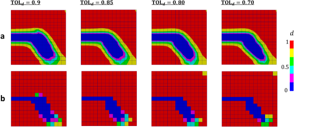
Figure 13: Example 1. Homogenized global crack phase-field solution for the isotropic single-edge-notched shear test (a) Global crack phase-field (b) Homogeneous crack phase-field solution at $\bar{\bm{u}}=0.0180\;mm$ for different $\texttt{TOL}_{d}$.

5.4 .Example 2: Analysis of transversely isotropic single-edge-notched tension test

The second example deals with transversely isotropic material responses under tension. It is based on different fiber directions given by the structural director $\bm{a}$ which is inclined under an angle $\phi$ with respect to the $x$-axis of a fixed Cartesian coordinate system. The numerical simulation is performed by applying a monotonic displacement $\bar{{\bm{\mathnormal{u}}}}=5\times 10^{-5}$ in vertical direction at the top of the specimen with a linearly increasing displacement. This loading setting is applied to the rest of numerical examples.

5.4.1 .Fiber direction of $\phi=+30^{\circ}$.

Here we investigate the transversely isotropic single-edge-notched tension test based on the fiber direction angle $\phi=+30^{\circ}$. We apply the Global-Local approach as follows:

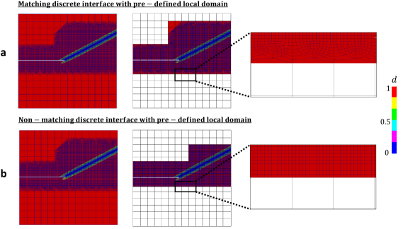
Figure 14: Example 2 (5.4.1). Transversely isotropic single-edge-notched tension with $\phi=+30^{\circ}$. Complete fracture state at $\bar{\bm{u}}=0.010\;mm$ for (a) matching discrete interface (Case a) $\Gamma_{G}=\Gamma_{L}$ and (b) non-matching discrete interface $\Gamma_{G}\neq\Gamma_{L}$ with predefined local domain (Case b).

• Case a. Without non-matching discrete interface and without adaptive scheme (a pre-defined local domain),

In this case, see Fig. 14a, we aim to evaluate the Proposition 1 such that ${\mathcal{B}}={\mathcal{B}}_{C}\cup\Gamma\cup{\mathcal{B}}_{L}$. Here, the local domain is predefined and no adaptivity is applied. Also, the discrete interface between the global and local domains are one to one such that $\Gamma_{G}=\Gamma_{L}$ (see Fig. 14a last column). It is clear that the two finite element meshes used for Global-Local approach represent ”precisely” the same as a single scale domain. Hence, we expect an identical Global-Local response compared with the single scale solutions (see Remark 1 in Appendix B). The complete fracture state is shown in Fig. 14a. Accordingly, a comparison of the load-displacement curves of the proposed formulation is demonstrated in Fig. 15a and shows a very good agreement compared with the single scale problem.

Remark 5.1.

Note that this case is similar to the work of Gerasimov et al. [34] if Robin-type boundary conditions are not taken into account (i.e. Global-Local approach based on Dirichlet-Neumann type boundary conditions), as sketched in Fig. 4a. Therein, the corresponding cumulative computational time is higher compared with the reference single scale solution (see Figure 10 in [34]), due to the slow convergence of the Global-Local procedure. That motivated the introduction of the Robin-type boundary conditions, resulting in a reduction of the computational cost, see Fig. 11b.

• Case b. With non-matching discrete interface and without adaptive scheme (a pre-defined local domain).

In the second case, we assume ${\mathcal{B}}\neq{\mathcal{B}}_{C}\cup\Gamma\cup{\mathcal{B}}_{L}$ and that the local domain is pre-defined hence no adaptivity is applied. Furthermore, the discrete interface between global and local domains are non-matching such that $\Gamma_{G}\neq\Gamma_{L}$ (see Fig. 14b last column). This removes one restriction applied in Case a, that is the matching discrete interface criteria.

The complete fracture state is shown in Fig. 14b. Compared with the first case, by the non-matching discrete interface, we are able to have an arbitrary mesh at the local domain (including interface) without any given interface conditions (and to avoid having distorted mesh between fine and coarse discretizations). The interface conditions refer to the identical discretization space for $\Gamma_{L}$ and $\Gamma_{G}$, see Remark 3.1. The importance can be observed when the fracture reaches the interface, see e.g. Fig. 9.

The resulting load-displacement curve in Fig. 15b has a very good agreement when compared with the single scale problem.

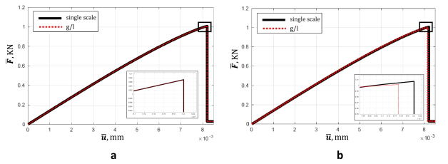
Figure 15: Example 2 (5.4.1). Transversely isotropic single-edge-notched tension with $\phi=+30^{\circ}$. Comparison of the load-displacement curve between single scale problem and Global-Local formulation. (a) Matching discrete interface with ${\mathcal{B}}={\mathcal{B}}_{C}\cup\Gamma\cup{\mathcal{B}}_{L}$ (Case a) and (b) non-matching discrete interface with ${\mathcal{B}}\neq{\mathcal{B}}_{C}\cup\Gamma\cup{\mathcal{B}}_{L}$ (Case b).

• Case c. With non-matching discrete interface and with adaptive scheme.

In the third case, we consider a non-matching discrete interface along with an adaptive scheme. This case removes all restrictions applied in Case a (matching interface and predefined local domain).

Fig. 16 illustrates the evolution of the crack phase-field along with the local domain and the corresponding Global-Local interface. The local domain and its coupling interface must be computed at each stage. The second row of Fig. 16 presents the local mesh evolution such that the non-matching discrete interface between global and local mesh is examined.

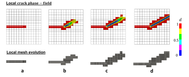
Figure 16: Example 2 (5.4.1 – Case c). Transversely isotropic single-edge-notched tension with $\phi=+30^{\circ}$. First row indicates the local crack phase-field resolution and second row represents the evolution of the local domain per time for different deformation states as follows: (a) $\bar{\bm{u}}=0.0030\;mm$ (b) $\bar{\bm{u}}=0.0088\;mm$ (c) $\bar{\bm{u}}=0.0092\;mm$ and (d) $\bar{\bm{u}}=0.010\;mm$.

To evaluate the solution related to the local to global transition, the load-displacement curve is shown in Fig. 17a. Since the single scale problem produces a very diffusive transition zone for the phase-field, more elements are involved (this is not the case in the sharp crack limit). This results in a small difference in the load-displacement curves between the Global-Local formulations and the reference single scale. Fig. 17b illustrates a reduction of the number of degrees of freedom.

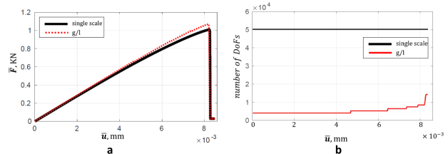
Figure 17: Example 2 (5.4.1 – Case c). Transversely isotropic single-edge-notched tension with $\phi=+30^{\circ}$. (a) Comparison of the load-displacement curve; (b) Number of degrees of freedom.

The Global-Local approach, besides its feasibility for having two ad-hoc finite element models for the global and local domain, enables computations with legacy codes. Additionally, the reduction of unknowns leads to a reduction of the computational time. To illustrate the time efficiency, the simulation time ratio between single scale and the Global-Local approach are shown in Fig. 18a. It can be observed that in average, the Global-Local formulations perform $12$ times faster. Furthermore, Fig. 18b demonstrates the corresponding accumulative computational time, which underlines the efficiency of the predictor-corrector adaptive scheme.

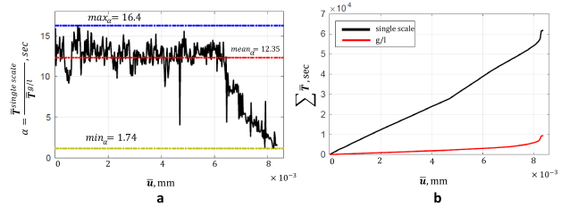
Figure 18: Example 2 (5.4.1 – Case c). Transversely isotropic single-edge-notched tension with $\phi=+30^{\circ}$. (a) Time ratio between the computed single scale and the Global-Local time per loading steps and (b) accumulated time-displacement curves.

Fig. 19a presents the total elastic strain energy per load increments. The resulting Global-Local curve is in a very good agreement with the single scale approach.

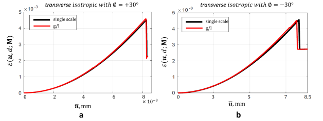
Figure 19: Example 2 (5.4.1 – Case c). Transversely isotropic single-edge-notched tension test. Comparison of the total energy functional between single scale domain and Global-Local scheme for fiber direction with $\phi=+30^{\circ}$ in (a) and fiber direction with $\phi=-30^{\circ}$ in (b).

Accordingly, the homogenized global phase-field solutions for different fracture states are depicted in Fig. 20. First and second row of Fig. 20 are based on approach (a) and (b) outlined in section 4.4. For comparison purposes, the single scale resolution is also plotted in the third row of Fig. 20. It is observed that, the homogenized phase-field solution in the case of the anisotropic setting, is able to capture the crack direction. The global phase-field solution is affected by the global element size and also $\texttt{TOL}_{d}$ (local scale).

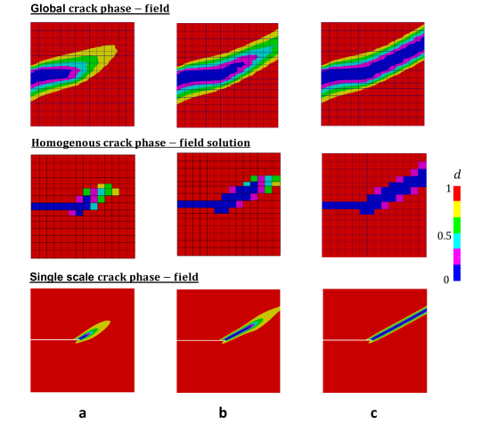
Figure 20: Example 2 (5.4.1 – Case c). Homogenized global crack phase-field solution for $\phi=+30$. First row: the global crack phase-field; Second row: the homogeneous solution; Third row: single scale phase field solution per loading step for different deformations states as: (a) $\bar{\bm{u}}=0.0088\;mm$ (b) $\bar{\bm{u}}=0.0092\;mm$ and (c) $\bar{\bm{u}}=0.010\;mm$.

5.4.2 .Fiber direction of $\phi=-30^{\circ}$.

This numerical example illustrates the transversely isotropic single-edge-notched tension test with $\phi=-30^{\circ}$. The crack phase-field resolution has a brutal fracture response in which a complete failure happens in one load increment. Thus the post-peak behavior is almost vertical, see Fig. 22. The aim of this numerical example is to show the capability of the Global-Local approach to capture such a brutal fracture behavior. This is mainly possible due to the introduction of the corrector step in the adaptive scheme described in Section 4.

Next, we investigate the effect of the $\texttt{TOL}_{d}$ in the case of the brutal fracture behavior, by setting $\texttt{TOL}_{d}=(0.90,0.80)$, as illustrated in Fig. 21. Similar as before, different $\texttt{TOL}_{d}$ lead to different fracture zones and hence different local domains. The crack paths for both $\texttt{TOL}_{d}=0.90$ and $\texttt{TOL}_{d}=0.80$ are identical, yet with $\texttt{TOL}_{d}=0.80$ a more narrow fracture zone is observed (hence a reduction of computational time).

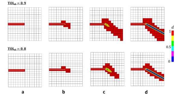
Figure 21: Example 2 (5.4.2). Fracture of transversely isotropic single-edge-notched plate under tension for $\phi=-30^{\circ}$. Resulting, local crack phase-field by Global-Local adaptive scheme indicated in; First row with $\texttt{TOL}_{d}=0.90$; Second row with $\texttt{TOL}_{d}=0.80$ per loading steps at (a) $\bar{\bm{u}}=0.0030\;mm$ (b) $\bar{\bm{u}}=0.0062\;mm$ (c) $\bar{\bm{u}}=0.0078\;mm$ (d) $\bar{\bm{u}}=0.0085\;mm$.

A comparison of the load-displacement curves are shown in Fig. 22a. The effect of $\texttt{TOL}_{d}$ on the load-displacement curve with zoom-in to the framed region of the left plot is shown in Fig. 22b. Despite of its brutal fracture behavior, the load-displacement curve with the higher value of $\texttt{TOL}_{d}=0.90$ has a good agreement when compared with a single scale solution.

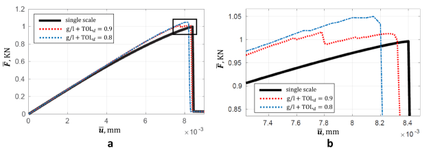
Figure 22: Example 2 (5.4.2). Effect of different $\texttt{TOL}_{d}$ on Global-Local approach by (a) Comparison of the load-displacement curve; (b) Zooming into the framed region of the left plot.

Following the approximation between the single scale and the Global-Local modeling, Fig. 19b presents a very good agreement in the total elastic strain energy of both schemes during the load increments.

Figure 23 describes the efficiency of the proposed Global-Local approach. Here the accumulative computational time is plotted in Fig. 23a and the number of unknowns are plotted in Fig. 23b versus the displacement and compared with the single scale domain. At each jump in Fig. 23b, the predictor-corrector adaptive scheme is active and applied on the Global-Local scheme which increases the number of degrees of freedoms.

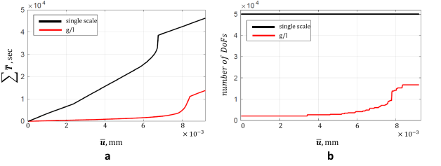
Figure 23: Example 2 (5.4.2). Time efficiency for the transversely isotropic single-edge-notched tension test (a) Time-displacement curves in terms of the accumulated time; (b) Number of degrees of freedom.

The homogenized global phase-field solution for this numerical setting is indicated in Fig. 24a at the complete fracture state. The single scale resolution is indicated in third row of Fig. 24b. It is evident that the homogenized phase-field solution is able to (i) capture the initial crack of the notch plate located at the local level and accordingly, (ii) the evolution of the fracture state which follows the preferred fiber direction.

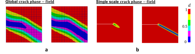
Figure 24: Example 2 (5.4.2). Homogenized global crack phase-field solution for $\phi=-30^{\circ}$. (a) Global crack phase-field and (b) single scale solution for two deformation states: $\bar{\bm{u}}=0.0078\;mm$ and $\bar{\bm{u}}=0.0085\;mm$.

5.5 .Example 3: Investigation of transversely isotropic heterogeneous L-shaped panel test

The third model problem is concerned with anisotropic brittle fracture of a heterogeneous L-shaped panel test. The homogeneous isotropic counterpart setting for this benchmark problem has been reported by many authors, see e.g. [64, 89, 6, 94]. We demonstrate the performance of the Global-Local approach to predict crack propagation without any given initial crack region. In this case the initial local domain needs to be determined based on the critical stress state at the global level as outlined in Fig 25c. To increase the order of complexity, a heterogeneous structure is considered by means of randomly distributed hard inclusions as plotted in Fig 25b. Furthermore transversely isotropic material behavior is assumed. The structural director $\bm{a}$ is inclined under $\phi=-15^{\circ}$.

Geometry and loading conditions are depicted in Fig. 25a. The size of the specimen is chosen to be: $A=B=250\;mm$ and $H=30\;mm$. The bottom edge of the specimen is fixed in both directions and a vertical displacement is applied until final failure, see Fig. 25a. One third of the specimen is covered by hard inclusions, as shown in Fig. 25b. Here, crack propagation is expected. The remaining parts of the domain are supposed to be homogeneous, but affected by the transversely isotropic behavior.

The material parameters used in the simulation are the same as in [89] and set as: $\lambda=6.16$ kN/mm², $\mu=10.95$ kN/mm², $G_{c}=9\times 10^{-5}$ kN/mm, $\alpha=\chi=50$ and $\Xi=0$. The dimensionless mismatch ratio is denoted by $m=E_{inclusion}/E_{matrix}$ (here, $E$ refers to Young’s modulus) and set as $m=10$. Thus, we deal with $E_{matrix}=25.85$ kN/mm² and $E_{inclusion}=258.5$ kN/mm².

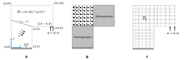
Figure 25: Example 3. Heterogeneous L-shaped panel test. (a) Geometry and loading setup with a structural director $\bm{a}$ inclined under an angle $\phi=-15$ (b) partitioning of domain into the heterogeneity and homogeneity counterparts and (c) global finite element mesh without potential fictitious zones.

In order to determine an initial fictitious domain, which has to be used for the Global-Local approach, an idea of the phase-field formulation with threshold state is considered. Here, a critical stress state on the global level is employed by extending the critical stress value of the isotropic phase-field formulation in [14] to an anisotropic heterogeneous setting. Hence, the critical values for the stress and corresponding strain, are obtained as

$${\bm{\varepsilon}}_{c}=\frac{\sqrt{3}}{3\,}\sqrt{\frac{G_{c}}{l\left(\mathrm{\chi}\,a^{4}+\bar{E}\right)}}\quad\mbox{and}\quad\bm{\sigma}_{c}=\frac{3\,\sqrt{3}}{16}{\sqrt{\frac{G_{c}\,\left(\mathrm{\chi}\,a^{4}+\bar{E}\right)}{l}}}.$$ (72)

This result is based on (34) and (71) where $a=\sin(\phi)$, see [88]. The effective Young’s modulus $\bar{E}$ for the heterogeneous domain is defined as

$$\bar{E}:=\frac{{E}_{Voigt}+{E}_{Reuss}}{2}$$

with

$${E}_{Voigt}:=\frac{1}{V}\int_{{\mathcal{B}}}E\,\mathrm{d}{{\bm{\mathnormal{x}}}},\;\;\mbox{and}\;\;{E}^{-1}_{Reuss}:=\frac{1}{V}\int_{{\mathcal{B}}}E^{-1}\,\mathrm{d}{{\bm{\mathnormal{x}}}}.$$

For $\chi=0$ in (72) the isotropic case of [14] is recovered. The critical stress state increases as $l$ decreases. Additionally, if the length scale $l$ goes to 0 in the limit, the crack nucleation stress tends to infinity. This is in agreement with Griffith’s theory, which allows to have crack nucleation in stress singularities. Then, the critical stresses based on the effective Young’s modulus $\bar{E}=36.136$ kN/mm² yields $\bm{\sigma}_{c}=9.2603$ N/mm² with the Voigt average ${E}_{Voigt}=44.423$ kN/mm² and the Reuss average ${E}_{Reuss}=27.850$ kN/mm².

Figure 26 shows the maximum stress state distribution of the heterogeneous L-shaped panel test. Here, the maximum stress is observed in the corner point of the specimen where the singularities are located. Hence, this is the potential candidate for the local domain. The Global-Local approach is then started after the stress state on the global domain reaches $75\%$ of $\bm{\sigma}_{c}$. This percentage of the critical stress is chosen to be on the safe side when starting the Global-Local formulations.

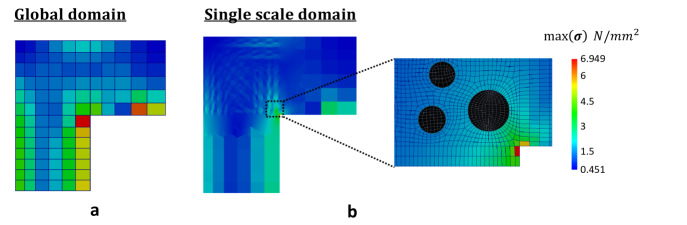
Figure 26: Example 3. Maximum stress state in the heterogeneous L-shaped panel test. (a) Global stress state and (b) single scale stress state.

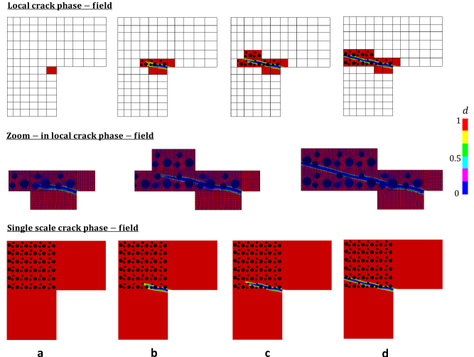
Figure 27: Example 3. Crack phase-field pattern for the transversely isotropic heterogeneous L-shaped panel test with fiber direction angle of $\phi=-15^{\circ}$. First row: local crack phase-field based on the adaptive scheme; Second row: mesh evolution for local domain by considering the influence of inclusions; Third row: resulting single scale phase-field solution at (a) $\bar{\bm{u}}=0.15\;mm$, (b) $\bar{\bm{u}}=0.324\;mm$, (c) $\bar{\bm{u}}=0.333\;mm$ and (d) $\bar{\bm{u}}=0.58\;mm$.

The evolution of the local crack phase-field with the corresponding mesh is depicted in Fig. 27 for different deformation stages. Specifically, the second row in Fig. 27 corresponds to the deformations $\bar{\bm{u}}=0.324\;mm$, $\bar{\bm{u}}=0.333\;mm$ and $\bar{\bm{u}}=0.58\;mm$, respectively. Due to the existing hard/stiff inclusions, the crack phase-field propagates around the inclusions. The resulting crack pattern indicated in Fig. 27 demonstrates an excellent agreement with the single scale simulation, with the advantage that the Global-Local approach requires significantly less degrees of freedom.

A comparison of the load-displacement curves is shown in Fig. 28a. Therein, a good agreement of the Global-Local approach with the single scale solution was observed for the heterogeneous L-shaped panel test. Figure 28b illustrates the efficiency of the Global-Local approach. Here the accumulative computational time is reduced by a factor of eight.

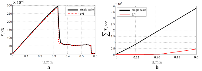
Figure 28: Example 3. Heterogeneous L-shaped panel test. (a) Comparison of the load-displacement curves and (b) accumulated time-displacement curves.

5.6 .Example 4: Investigation of transversely isotropic double-edge-notched tension

The last example is concerned with the capability of the proposed Global-Local approach for handling coalescence and merging of crack paths in the local domains. Specifically, the following numerical test aims to illustrate the effects of the double notch shaped specimen. Here crack-initiation and curved-crack-propagation, representing a mixed-mode fracture, are predicted with a Global-Local formulation. Additionally a transversely isotropic material behavior given by the structural director $\bm{a}$ that is inclined under $\phi=-15^{\circ}$ is assumed.

The geometrical setup and the loading conditions of the notched specimen is depicted in Fig. 29a. The bottom edge of the plate is fixed in the $x$ and $y$ directions. A vertical displacement is applied at the top edge until final failure. We set $A=20\;mm$ and $B=10\;mm$ hence ${\mathcal{B}}=(20,10)^{2}$ $mm^{2}$. For the double-edge-notches, let $H_{1}=5.5\;mm$ and $H_{2}=3.5\;mm$ with the predefined crack length of $l_{0}=5\;mm$, see Fig. 29a. The material parameters used in the simulation are the same as in [2] and set as: $\lambda=12$ kN/mm², $\mu=8$ kN/mm², $G_{c}=1\times 10^{-3}$ kN/mm, $\alpha=\chi=50$ and $\Xi=0$.

The global finite element mesh includes two potential fictitious zones ${\mathcal{B}}_{F,1}$ and ${\mathcal{B}}_{F,2}$ with the interfaces $\Gamma_{1}$ and $\Gamma_{2}$ shown in Fig, 29b.

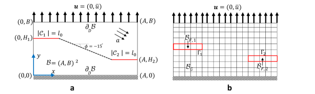
Figure 29: Example 4. Double-edge-notched tensile test. (a) Geometry and loading setup with a structural director $\bm{a}$ inclined under an angle $\phi=-15$ and (b) global finite element mesh with two potential fictitious zone ${\mathcal{B}}_{F,1}$ and ${\mathcal{B}}_{F,2}$.

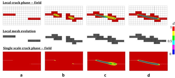
Figure 30: Example 4. Crack phase-field pattern for transversely isotropic double-edge-notched plate under tension with fiber direction angle of $\phi=-15^{\circ}$. First row: local crack phase-field based on the adaptive scheme; Second row: mesh evolution for local domain; Third row: resulting single scale phase-field solution at (a) $\bar{\bm{u}}=0.01\;mm$, (b) $\bar{\bm{u}}=0.0122\;mm$, (c) $\bar{\bm{u}}=0.0143\;mm$ and (d) $\bar{\bm{u}}=0.0145\;mm$.

The evolution of the crack phase-field resulting from the local domain along with its mesh evolution are indicted in Fig. 30 for different deformation stages up to final failure. The single scale crack phase-field simulation is shown in Fig. 30 in the third row. At the loading step $\bar{\bm{u}}=0.0143\;mm$ the coalescence and merging of the two local domains are observed. Furthermore, a considerable reduction of the unknowns versus the single scale problem, can be clearly noticed due to the very narrow ${\mathcal{B}}_{L}$ in Fig. 30.

These results demonstrate the feasibility/efficiency of using the proposed adaptive Global-Local approach for different local domains and more complicated structures.

6 .Conclusion

In this work, we developed a robust and efficient Global-Local approach for treating phase-field fracture problems. Anisotropic heterogeneous materials, due to the highly oscillating response on the local level, often require multi-scale treatments such that the full resolution on the local scale must be taken into account. Multi-scale approaches are advantageous when large-scale problems are considered in which the fracture state only develops in smaller, localized, regions. Our first aim was to extend the phase-field model to anisotropic constitutive laws. Next, we developed an adaptive scheme in which the local domains are advanced dynamically during a computation. This approach is realized in terms of a predictor-corrector scheme. First, the new local domains are predicted and then the solution is again computed considering the new local regions. An important challenge are interface conditions for the coupling of the two-nested models denoted by the local and global domains in a variational consistent way. For that purpose Robin-type boundary conditions were formulated. Moreover, non-matching grids are allowed such that the local and global domains can be updated independently of any additional conditions on the mesh. Several numerical examples are presented to substantiate our algorithmic developments. Here, we considered isotropic and anisotropic constitutive materials equations. The focus was on crack patterns, load-displacement curves and investigations of the thermodynamic consistency in terms of the energy functional, the efficiency of the adaptive schemes and the choice of different threshold values for detecting the local domain. The overall response of the Global-Local approach in terms of accuracy, robustness and efficiency for the two nested finite element models was verified using single scale problems. In all examples, an excellent performance of the proposed framework was observed.

Acknowledgment

NN was partially supported by the Priority Program DFG - SPP 1748 under the project WI 4367/2-1. FA was founded by the Priority Program DFG - SPP 2020 under the project WR 19/58-1. TW and PW were funded by the Deutsche Forschungsgemeinschaft (DFG, German Research Foundation) under Germany’s Excellence Strategy within the Cluster of Excellence PhoenixD (EXC 2122), project ID 390833453.

Appendix A. Finite Element Discretization

Let $\mathcal{P}$ be a finite element partition of ${\mathcal{B}}$ into quadrilaterals, and $N_{i}$ denotes the nodal shape function associated with the node $i$. The scalar-valued quantity $\hat{\bullet}_{i}$ represents the nodal value. For the global-local formulation, we assume the existence of the partitions $\mathcal{P}_{G}$ and $\mathcal{P}_{L}$. The solution discretization are given by

$$\bm{u}_{G}=\bm{N}_{u}^{G}\hat{\bm{u}}_{G},\quad\bm{u}_{L}=\bm{N}_{u}^{L}\hat{\bm{u}}_{L},\quad d_{L}=\bm{N}_{d}^{L}\hat{\bm{d}}_{L},$$ (A.1)

and its derivative

$$\bm{\varepsilon}(\bm{u}_{G})=\bm{B}_{u}^{G}\hat{\bm{u}}_{G},\quad\bm{\varepsilon}(\bm{u}_{L})=\bm{B}_{u}^{L}\hat{\bm{u}}_{L},\quad\nabla d_{L}=\bm{B}_{d}^{L}\hat{\bm{d}}_{L}.$$ (A.2)

To construct the discretization of the Lagrange multipliers $\bm{\lambda}_{C}$, $\bm{\lambda}_{L}$, $\bm{u}_{\Gamma}$ and the supplementary quantity $\bm{\lambda}_{F}$ on $\Gamma$, we write

$$\bm{\lambda}_{C}=\bm{N}_{\lambda}^{G}\hat{\bm{\lambda}}_{C},\quad\bm{\lambda}_{L}=\bm{N}_{\lambda}^{L}\hat{\bm{\lambda}}_{L},\quad\bm{u}_{\Gamma}=\bm{N}_{u}^{\Gamma}\hat{\bm{u}}_{\Gamma},\quad\bm{\lambda}_{F}=\bm{N}_{\lambda}^{G}\hat{\bm{\lambda}}_{F}.$$ (A.3)

We assume that $\bm{N}_{\lambda}^{G}=\bm{N}_{u}^{G}=\bm{N}_{u}^{\Gamma}$ and $\bm{N}_{\lambda}^{L}:=\bm{N}_{u}^{L}$. This discretization for the Lagrange multipliers satisfies the inf-sup condition, see e.g. [96, 97].

Thus, coupling terms are discretized by

$${{\bf{J}}_{G}=\int_{{\mathit{{\mathcal{B}}}}_{G}}({{\bm{N}_{\lambda}^{G}})^{T}{\bm{N}_{u}^{G}}\ \mathrm{d}{{\bm{\mathnormal{x}}}}},\ \ \;\;\;\;{\bf{J}}_{L}=\int_{{\mathit{{\mathcal{B}}}}_{L}}({{\bm{N}_{\lambda}^{L}})^{T}{\bm{N}_{u}^{L}}\ {\,\mathrm{d}{{\bm{\mathnormal{x}}}}}}},$$ (A.4)

$${{\bf{L}}_{G}=\int_{{\Gamma}_{G}}({\bm{N}_{\lambda}^{G}})^{T}{\bm{N}_{u}^{\Gamma}}\ {\mathrm{d}s}},\ \ \;\;\;\;{{\bf{L}}_{L}=\int_{{\Gamma}_{L}}({\bm{N}_{\lambda}^{L}})^{T}{\bm{N}_{u}^{\Gamma}}\ {\mathrm{d}s}}.$$

Following our discretization, ${\bf{J}}_{G}:{\mathcal{B}}_{G}\rightarrow\Gamma_{G}$ and ${\bf{J}}_{L}:{\mathcal{B}}_{L}\rightarrow\Gamma_{L}$ become signed Boolean mappings [12] which are used to project the entire domain to interface contributions, such that

$${\hat{\bm{u}}_{G,b}}:={\bf{J}}_{G}{\hat{\bm{u}}_{G}}\quad\mathchoice{\hbox{{and}}}{\hbox{{and}}}{\hbox{{and}}}{\hbox{{and}}}\quad{\hat{\bm{u}}_{L,b}}:={\bf{J}}_{L}{\hat{\bm{u}}_{L}}.$$ (A.5)

Here, $b$ are denoted as interface nodes. In order to handle a non-matching finite element discretization on the interface, more specifically to compute ${\bf L}_{L}$ and ${\bf L}_{G}$, a dual mortar method [96] is implemented. This provides sufficient regularity of the underlying FE meshes.

Appendix B. Derivation of Robin-Type Boundary conditions

In this section, we investigate the relationship between ${\Delta{\hat{\bm{u}}}}$ and $\Delta{\hat{\bm{\lambda}}}$ (in the incremental sense) for the complementary, fictitious and local domain at the converged solution state. Doing that, Robin-type boundary conditions can be derived such that all coupling terms given in (C₁), (C₂) and (C₃) satisfied, simultaneously, at a Global-Local iteration $k$.

Recall the complementary term used in Eq. 48 and let $\bm{u}_{C}$ and $\bm{\lambda}_{C}$ be the stationary of the following functional,

$${\mathcal{L}}={\mathcal{L}}({\bm{u}}_{C},\bm{\lambda}_{C};{\bm{\mathnormal{M}}}):=\int_{{\mathcal{B}}_{C}}w({\bm{\varepsilon}}_{C},1,1;{\bm{\mathnormal{M}}})\,\mathrm{d}{\bm{x}}+\int_{\Gamma}\bm{\lambda}_{C}\cdot({{\bm{u}}_{\Gamma}}-{\bm{u}}_{C})\,\mathrm{d}s-\int_{\Gamma_{N,C}}{\bm{\bar{\tau}}}\cdot\bm{u}_{C}\,\mathrm{d}s.$$ (B.1)

Here, $\Gamma\in\mathbb{R}^{\delta-1}\subset{\mathcal{B}}_{C}$ is denoted as an interface and $\;{{\bm{u}}_{\Gamma}}:=\mbox{tr}\;{\bm{u}}_{C}\in{\bf H}^{1/2}(\Gamma)$ can be given implicitly, i.e. ($\widetilde{\text{C}}_{1}$)$+$($\widetilde{\text{C}}_{2}$) or explicitly, i.e. ($\widetilde{\text{C}}_{4}$). Recall Eq. B.1 lives in ${\mathcal{B}}_{C}$ (the following description holds true for ${\mathcal{B}}_{F}$ except ${\bm{\bar{\tau}}}={\bm{0}}$). The stationary points of the energy functional for the ${\mathcal{L}}$ is characterized by the first-order necessary conditions through ${\bf{\mathcal{L}}_{1}}={{\mathcal{L}}_{\bm{u}}({\bm{u}}_{C},\bm{\lambda}_{C};{\bm{w}})=\bm{0}}\;\mbox{and}\;{{\bf{\mathcal{L}}_{2}}={\mathcal{L}}_{\bm{\lambda}}({\bm{u}}_{C},\bm{\lambda}_{C};{\bm{\kappa}})=\bm{0}}$. We split ${\bf{\mathcal{L}}_{1}}$ into inner nodes and interface nodes denoted as, $\{a,\;b\}$, respectively, by

$${{{\bf{\mathcal{L}}}^{a}_{1}}({\bm{u}})={\bm{\texttt{f}}^{\>a}}-{\bar{\bf F}}\overset{!}{=}{\bm{0}}}\quad\;\quad\;\;{\bm{x}\in{\mathcal{B}}\backslash\Gamma},$$ (B.2)

$${{{\bf{\mathcal{L}}}^{b}_{1}}({\bm{u}}){=}{\bm{\texttt{f}}^{\>b}-{{\bf{L}}^{T}_{G}}{\hat{\bm{\lambda}}}_{C}}\overset{!}{=}{\bm{0}}}\quad\;\;{\bm{x}\in\Gamma},$$

$${\bf{\mathcal{L}}_{2}}={{\bf{L}}_{G}}\hat{\bm{u}}_{\Gamma}-{{\bf{J}}_{G}}{\hat{\bm{u}}_{C}}\overset{!}{=}{\bm{0}}\;\;\;\;{\bm{x}\in\Gamma}.$$

Here, ${\bm{\texttt{f}}}=\displaystyle\int_{{\mathcal{B}}}{(\bm{B}_{u}^{G})^{T}}{\bm{\sigma}}({{\bm{u}}_{C}})\,\mathrm{d}{\bm{x}}$ is an internal nodal force vector and $\bar{{\bf F}}=\displaystyle\int_{\Gamma_{N}}{(\bm{N}_{u}^{G})^{T}}{\bm{\bar{\tau}}}\,\mathrm{d}{s}$ stands for the external force vector. It is trivial that the Lagrange multiplier acts as an external force on the interface. A Newton-type solution for the residual based system of equations for $({\bm{u}}_{C},\bm{\lambda}_{C})$ is provided by the linearization

$${({\bm{\texttt{f}}^{\>a}}-{\bar{\bf F}})+{{\bf K}_{aa}}{\Delta{\hat{\bm{u}}}_{C,a}}+{{\bf K}_{ab}}{\Delta{\hat{\bm{u}}}_{C,b}}={\bm{0}}},$$ (B.3)

$${({\bm{\texttt{f}}^{\>b}-{{\bf{L}}^{T}_{G}}{\hat{\bm{\lambda}}_{C}}})+{{\bf K}_{ba}}{\Delta{\hat{\bm{u}}}_{C,a}}+{{\bf K}_{bb}}{\Delta{{\hat{\bm{u}}}}_{C,b}}-{{\bf{L}}^{T}_{G}}{\Delta\hat{\bm{\lambda}}_{C}}={\bm{0}}},$$

$$({{\bf{L}}_{G}}{{\hat{\bm{u}}}}_{\Gamma}-{{\bf{L}}_{G}}{\Delta{{\hat{\bm{u}}}}_{b}})+{{\bf{L}}_{G}}{\Delta{\hat{\bm{u}}}}_{\Gamma}-{{\bf{L}}_{G}}{\Delta{{\hat{\bm{u}}}}_{C,b}}=0.$$

where ${\bf K}:={\partial{\bm{\texttt{f}}}}/{\partial{\hat{\bm{u}}_{C}}}$ is the standard tangent stiffness matrix. Here, we have the following iterative update

$${{\hat{\bm{u}}}}_{C,a}\leftarrow{{\hat{\bm{u}}}}_{C,a}+{\Delta{{\hat{\bm{u}}}}_{C,a}},\;\;{{\hat{\bm{u}}}}_{C,b}\leftarrow{{\hat{\bm{u}}}}_{C,b}+{\Delta{{\hat{\bm{u}}}}_{C,b}},\;\;\mbox{and}\;\;{\hat{\bm{\lambda}}_{C}}\leftarrow{\hat{\bm{\lambda}}_{C}}+{\Delta{\hat{\bm{\lambda}}}_{C}}.$$ (B.4)

Let us assume that the equilibrium state is achieved such that ${{\bf{\mathcal{L}}}^{a}_{1}}={\bm{0}},{{\bf{\mathcal{L}}}^{b}_{1}}={\bm{0}}$ and ${\bf{\mathcal{L}}_{2}}={\bm{0}}$. Thus, Eq. B.3 takes the form

$${\bm{\mathcal{S}}_{C}}{\Delta{\hat{\bm{u}}}}_{C,b}={\bm{\mathcal{S}}_{C}}{\Delta{\hat{\bm{u}}}}_{\Gamma}=:{{\bf{L}}^{T}_{G}}{\Delta{\hat{\bm{\lambda}}}_{C}}\quad\mbox{with}\quad{\bm{\mathcal{S}}}_{C}:={\bm{\mathcal{S}}}({\bf K}_{C})={\bf K}_{bb}-{\bf K}_{bba}{\bf K}^{-1}_{aa}{\bf K}_{ab},$$ (B.5)

where ${\bm{\mathcal{S}}}$ refers to the Steklov-Poincaré mapping [50]. By means of Eq. B.5, displacement ${\hat{\bm{u}}_{C}}$ is extracted from the interface $\Gamma$ and through the Poincaré-Steklov mapping ${\bm{\mathcal{S}}}$ returns the outward normal stress derivative with respect to the trace of the displacement. That is called Dirichlet-to-Neumann mapping [22, 36].

In a similar way, we have the following identity

$${\bm{\mathcal{S}}_{L}}{\Delta{\hat{\bm{u}}}}_{L,b}={{\bf{T}}^{T}_{L}}{\Delta{\hat{\bm{\lambda}}_{L}}}\quad\mbox{and}\quad{\bm{\mathcal{S}}_{F}}{\Delta{\hat{\bm{u}}}}_{F,b}={{\bf{L}}^{T}_{G}}{\Delta{\hat{\bm{\lambda}}}_{F}}.$$ (B.6)

Here, ${{\bf{T}}_{L}}:={\bf{J}}_{L}|_{\Gamma_{L}}$ is the restriction of ${\bf{J}}_{L}$ from ${\mathcal{B}}_{L}$ to $\Gamma_{L}$. Furthermore, we define ${\bm{\mathcal{S}}_{L}}:={\bm{\mathcal{S}}}({\bf K}_{L})$ and ${\bm{\mathcal{S}}_{F}}:={\bm{\mathcal{S}}}({\bf K}_{F})$ in Eq. B.6.

Proposition 1.

Let the global solutions be at the converged state and let the following identity holds true:

$$\bm{u}_{\Gamma}^{k,\frac{1}{2}}=\bm{u}_{\Gamma}^{k}\;\in\;\Gamma,$$ (B.7)

then the Global-Local formulation is converged. In addition, (B.7) holds true if and only if

$$\Delta{\bm{\Lambda}}_{L}={\bm{\Lambda}}^{k}_{L}-{\bm{\Lambda}}^{k-1}_{L}=0.$$ (B.8)

Proof. The proof constitutes of two parts. Note, the Global-Local procedure is in the convergence state if, all the coupling terms (C₁), (C₂) and (C₃) holds true at iteration $k$.

(a) Let condition $\bm{u}_{\Gamma}^{k,\frac{1}{2}}=\bm{u}_{\Gamma}^{k}$ hold, then it is evident (C₂) and (C₃) are satisfied in iteration $k$. Accordingly, replacing Eq. 62 in ($\widetilde{\text{C}}_{3}$) yields

$$\int_{\Gamma}(\bm{\lambda}^{k}_{C}+\bm{\lambda}^{k}_{L})\cdot\delta{\bm{u}}_{\Gamma}\,\mathrm{d}s+{\IKbb A}_{G}\int_{\Gamma}(\bm{u}_{\Gamma}^{k}-\bm{u}^{k}_{L})\cdot{\delta{\bm{\lambda}}_{L}}\,\mathrm{d}s=0,$$ (B.9)

where the second term due to ($\widetilde{\text{C}}_{2}$) and the identity of $\bm{u}_{\Gamma}^{k,\frac{1}{2}}=\bm{u}_{\Gamma}^{k}$ becomes zero. Hence this results in the continuity of tractions at iteration $k$, i.e. (C₁) is satisfied.

(b) Let $\Delta{\bm{\Lambda}}_{L}={\bm{\Lambda}}^{k}_{L}-{\bm{\Lambda}}^{k-1}_{L}=0$ hold, then (60) can be restated as

$${\bm{\Lambda}}^{k-1}_{L}={\bm{\Lambda}}^{k}_{L} ={\IKbb A}_{L}\int_{\Gamma}\bm{u}_{G}^{k}\cdot{\delta{\bm{\lambda}}_{C}}\,\mathrm{d}s-\int_{\Gamma}\bm{\lambda}^{k}_{C}\cdot\bm{v}_{\Gamma}\,\mathrm{d}s,$$ (B.10)

and therefore ($\widetilde{\text{C}}_{1}$) is restated as,

$$\int_{\Gamma}(\bm{\lambda}^{k}_{C}+\bm{\lambda}^{k}_{L})\cdot{\delta{\bm{u}}_{\Gamma}}\,\mathrm{d}s+{\IKbb A}_{L}\int_{\Gamma}(\bm{u}_{\Gamma}^{k,\frac{1}{2}}-\bm{u}^{k}_{G})\cdot{\delta{\bm{\lambda}}_{C}}\,\mathrm{d}s=\int_{\Gamma}(\bm{\lambda}^{k}_{C}+\bm{\lambda}^{k}_{L})\cdot{\delta{\bm{u}}_{\Gamma}}\,\mathrm{d}s=0,$$ (B.11)

where ($\widetilde{\text{C}}_{4}$) is used. Subtracting Eq. B.11 from ($\widetilde{\text{C}}_{3}$) yields

$${\IKbb A}_{G}\int_{\Gamma}(\bm{u}_{\Gamma}^{k}-\bm{u}^{k}_{L})\cdot{\delta{\bm{\lambda}}_{L}}\,\mathrm{d}s={\IKbb A}_{G}\int_{\Gamma}(\bm{u}_{\Gamma}^{k}-\bm{u}_{\Gamma}^{k,\frac{1}{2}})\cdot{\delta{\bm{\lambda}}_{L}}\,\mathrm{d}s=0,$$ (B.12)

which results in $\bm{u}_{\Gamma}^{k}=\bm{u}_{\Gamma}^{k,\frac{1}{2}}$ . Herein, Eq. $\widetilde{\text{C}}_{2}$ is used. Reciprocally, if $\bm{u}_{\Gamma}^{k,\frac{1}{2}}=\bm{u}_{\Gamma}^{k}\;\in\;\Gamma$ satisfied then $\Delta{\bm{\Lambda}}_{L}=0$ holds. The proof is left for the readers.  

Remark B.1. Let the Global-Local approach be in the converged state such that $\bm{u}_{\Gamma}^{k,\frac{1}{2}}=\bm{u}_{\Gamma}^{k}\;\in\;\Gamma$. We underline if ${\mathcal{B}}={\mathcal{B}}_{C}\cup\Gamma\cup{\mathcal{B}}_{L}$ holds, then the Global-Local mesh compared with a single scale mesh is one to one, and the resulting Global-Local solutions are identical with the single scale solutions. This is because the two finite element meshes which correspond to the complementary and local domains are ‘exactly’ identical to the single scale mesh; we refer the reader to Section 5.4.1 for case a.

We now determine specific Robin-type boundary conditions such that $\Delta{\bm{\Lambda}}_{L}=0$ holds which results in $\bm{u}_{\Gamma}^{k}=\bm{u}_{\Gamma}^{k,\frac{1}{2}}$ by means of Proposition 1 and that yields the Global-Local iterative process to be in the converged state.

Recall (60) and find ${\IKbb A}_{L}$ such that $\Delta{\bm{\Lambda}}_{L}={\bm{\Lambda}}^{k}_{L}-{\bm{\Lambda}}^{k-1}_{L}=0$. Hence we have,

$$\Delta{\bm{\Lambda}}_{L}={\IKbb A}_{L}\int_{\Gamma}\Delta\bm{u}_{G}\cdot{\delta{\bm{\lambda}}_{C}}\,\mathrm{d}s-\int_{\Gamma}\Delta\bm{\lambda}_{C}\cdot{\delta{\bm{u}}_{\Gamma}}\,\mathrm{d}s=0,$$ (B.13)

resulting to

$${\IKbb A}_{L}\int_{\Gamma}\Delta\bm{u}_{G}\cdot{\delta{\bm{\lambda}}_{C}}\,\mathrm{d}s=\int_{\Gamma}\Delta\bm{\lambda}_{C}\cdot{\delta{\bm{u}}_{\Gamma}}\,\mathrm{d}s\;\;\rightarrow\;\;{\IKbb A}_{L}{\bf{J}}_{G}{\Delta\hat{\bm{u}}_{G}}={{\bf{L}}^{T}_{G}}{\Delta\hat{\bm{\lambda}}_{C}},$$ (B.14)

By means of (B.5) and considering (A.5)₁, this equality holds if ${\IKbb A}_{L}:={\bm{\mathcal{S}}}_{C}$ which is the Dirichlet-to-Neumann operator assigned to $\Gamma_{G}\in{\mathcal{B}}_{C}$.

In a similar manner, let us find ${\IKbb A}_{G}$ such that $\Delta{\bm{\Lambda}}_{G}={\bm{\Lambda}}^{k}_{G}-{\bm{\Lambda}}^{k-1}_{G}=0$. This yields

$${\IKbb A}_{G}\int_{\Gamma}\Delta\bm{u}_{L}\cdot{\delta{\bm{\lambda}}_{L}}\,\mathrm{d}s=\int_{\Gamma}\Delta\bm{\lambda}_{L}\cdot{\delta{\bm{u}}_{\Gamma}}\,\mathrm{d}s\;\;\rightarrow\;\;{\IKbb A}_{G}{\bf{J}}_{L}{\Delta\hat{\bm{u}}_{L}}={{\bf{L}}^{T}_{L}}{\Delta\hat{\bm{\lambda}}_{L}}.$$ (B.15)

By means of (B.6)₁ and (A.5)₂, we have ${\IKbb A}_{G}={\bm{L}^{T}_{L}}{\bm{T}^{-T}_{L}}{\bm{\mathcal{S}}}_{L}$. Based on Proposition 1 the converged state of the Global-Local iteration is independent of the choice of ${\IKbb A}_{G}$ hence one can simply replace ${\bm{\mathcal{S}}}_{L}$ by the identity tensor. Hence, there is no need to access ${\bm{\mathcal{S}}}_{L}$ at the global level.

References

- Aldakheel et al. [2014] Aldakheel, F.; Mauthe, S.; Miehe, C. [2014]: Towards phase field modeling of ductile fracture in gradient-extended elastic-plastic solids. Proceedings in Applied Mathematics and Mechanics, 14: 411–412.
- Aldakheel et al. [2018a] Aldakheel, F.; Hudobivnik, B.; Hussein, A.; Wriggers, P. [2018]: Phase-field modeling of brittle fracture using an efficient virtual element scheme. Computer Methods in Applied Mechanics and Engineering, 341: 443–466.
- Aldakheel et al. [2018b] Aldakheel, F.; Hudobivnik, B.; Wriggers, P. [2018]: Virtual element formulation for phase-field modeling of ductile fracture. International Journal for Multiscale Computational Engineering. DOI: 10.1615/IntJMultCompEng.2018026804.
- Aldakheel [2016] Aldakheel, F. [2016]: Mechanics of Nonlocal Dissipative Solids: Gradient Plasticity and Phase Field Modeling of Ductile Fracture. Ph.D. Thesis, Institute of Applied Mechanics (CE), Chair I, University of Stuttgart. http://dx.doi.org/10.18419/opus-8803.
- Aldakheel et al. [2018c] Aldakheel, F.; Wriggers, P.; Miehe, C. [2018]: A modified gurson-type plasticity model at finite strains: Formulation, numerical analysis and phase-field coupling. Computational Mechanics, 62: 815–833.
- Ambati et al. [2015] Ambati, M.; Gerasimov, T.; De Lorenzis, L. [2015]: A review on phase-field models of brittle fracture and a new fast hybrid formulation. Computational Mechanics, 55(2): 383–405.
- Ambrosio & Tortorelli [1990] Ambrosio, L.; Tortorelli, V. [1990]: Approximation of functionals depending on jumps by elliptic functionals via -convergence. Communications on Pure and Applied Mathematics, 43: 999–1036.
- Ambrosio & Tortorelli [1992] Ambrosio, L.; Tortorelli, V. [1992]: On the approximation of free discontinuity problems. Bollettino dell’Unione Matematica Italiana, 6: 105–123.
- Amor et al. [2009] Amor, H.; Marigo, J.; Maurini, C. [2009]: Regularized formulation of the variational brittle fracture with unilateral contact: Numerical experiments. Journal of the Mechanics and Physics of Solids, 57: 1209–1229.
- Balzani et al. [2006] Balzani, D.; Neff, P.; Schröder, J.; Holzapfel, G. [2006]: A polyconvex framework for soft biological tissues. adjustment to experimental data. International Journal of Solids and Structures, 43: 6052–6070.
- Bangerth et al. [2007] Bangerth, W.; Hartmann, R.; Kanschat, G. [2007]: deal.II – a general purpose object oriented finite element library. ACM Transactions on Mathematical Software, 33(4): 24/1–24/27.
- Belytschko et al. [2014] Belytschko, T.; Liu, W. K.; Moran, B.; Elkhodary, K. [2014]: Nonlinear Finite Elements for Continua and Structure. John Wiley and Sons, Ltd., United Kingdom.
- Bleyer & Alessi [2018] Bleyer, J.; Alessi, R. [2018]: Phase-field modeling of anisotropic brittle fracture including several damage mechanisms. Computer Methods in Applied Mechanics and Engineering. https://doi.org/10.1016/j.cma.2018.03.012.
- Borden et al. [2012] Borden, M. J.; Verhoosel, C. V.; Scott, M. A.; Hughes, T. J. R.; Landis, C. M. [2012]: A phase-field description of dynamic brittle fracture. Computer Methods in Applied Mechanics and Engineering, 217-220: 77–95.
- Bourdin [1999] Bourdin, B. [1999]: Image segmentation with a finite element method. Mathematical Modelling and Numerical Analysis, 33(2): 229–244.
- Bourdin [2007] Bourdin, B. [2007]: Numerical implementation of the variational formulation for quasi-static brittle fracture. Interfaces and free boundaries, 9: 411–430.
- Bourdin et al. [2000] Bourdin, B.; Francfort, G.; Marigo, J.-J. [2000]: Numerical experiments in revisited brittle fracture. Journal of the Mechanics and Physics of Solids, 48(4): 797–826.
- Bourdin et al. [2008] Bourdin, B.; Francfort, G.; Marigo, J.-J. [2008]: The variational approach to fracture. Journal of Elasticity, 91: 5–148.
- Chapman [2003] Chapman, S. J. [2003]: Fortran 90/95 for Scientists and Engineers. McGraw-Hill, Inc., New York, NY, USA, 2 Edition.
- Chevreuil et al. [2013] Chevreuil, M.; Nouy, A.; Safatly, E. [2013]: A multiscale method with patch for the solution of stochastic partial differential equations with localized uncertainties. Computer Methods in Applied Mechanics and Engineering, 255: 255–274.
- Ciarlet [1987] Ciarlet, P. G. [1987]: The finite element method for elliptic problems. North-Holland, Amsterdam [u.a.], 2. pr. Edition.
- Deparis et al. [2007] Deparis, S.; Discacciati, M.; Fourestey, G.; Quarteroni, A. [2007]: Heterogeneous domain decomposition methods for fluid-structure interaction problems. Domain Decomposition Methods in Science and Engineering XVI. Lecture Notes in Computational Science and Engineering, 55: 41–52.
- Dittmann et al. [2018] Dittmann, M.; Aldakheel, F.; Schulte, J.; Wriggers, P.; Hesch, C. [2018]: Variational phase-field formulation of non-linear ductile fracture. Computer Methods in Applied Mechanics and Engineering, 342: 71–94.
- Donath [1961] Donath, F. A. [1961]: Experimental study of shear failure in anisotropic rocks. GSA Bulletin, 72(6): 985–989.
- Farhat & Roux [1991] Farhat, C.; Roux, F. [1991]: A method of finite element tearing and interconnecting and its parallel solution algorithm. International Journal for Numerical Methods in Engineering, 32: 1205–1227.
- Farhat et al. [2000] Farhat, C.; Macedo, A.; Lesoinne, M.; Roux, F.-X.; Magoulés, F.; Bourdonnaie, A. D. L. [2000]: Two-level domain decomposition methods with lagrange multipliers for the fast iterative solution of acoustic scattering problems. Computer Methods in Applied Mechanics and Engineering, 184: 213–239.
- Farrell & Maurini [2017] Farrell, P. E.; Maurini, C. [2017]: Linear and nonlinear solvers for variational phase-field models of brittle fracture. International Journal for Numerical Methods in Engineering, 109: 648–667.
- Fish & Wagiman [1993] Fish, J.; Wagiman, A. [1993]: Multiscale finite element method for a locally nonperiodic heterogeneous medium. Computational Mechanics, 12(3): 164–180.
- Fish [2014] Fish, J. [2014]: Practical Multiscaling. John Wiley and Sons, Ltd., United Kingdom.
- Francfort & Marigo [1998] Francfort, G.; Marigo, J.-J. [1998]: Revisiting brittle fracture as an energy minimization problem. Journal of the Mechanics and Physics of Solids, 46(8): 1319–1342.
- Gander et al. [2007] Gander, M.; Halpern, L.; Magoules, F. [2007]: An optimized schwarz method with two-sided robin transmission conditions for the helmholtz equation. International Journal for Numerical Methods in Fluids, 55: 163–175.
- Gendre et al. [2009] Gendre, L.; Allix, O.; Gosselet, P.; Comte, F. [2009]: Non-intrusive and exact global/local techniques for structural problems with local plasticity. Computational Mechanics, 44: 233–245.
- Gendre et al. [2011] Gendre, L.; Allix, O.; Gosselet, P. [2011]: A two-scale approximation of the schur complement and its use for non-intrusive coupling. International Journal for Numerical Methods in Engineering, 87: 889–905.
- Gerasimov et al. [2018] Gerasimov, T.; Noii, N.; Allix, O.; De Lorenzis, L. [2018]: A non-intrusive global/local approach applied to phase-field modeling of brittle fracture. Advanced Modeling and Simulation in Engineering Sciences. https://doi.org/10.1186/s40323-018-0105-8.
- Gosselet & Rey [2006] Gosselet, P.; Rey, C. [2006]: Non-overlapping domain decomposition methods in structural mechanics. Archives of Computational Methods in Engineering, 13: 515–572.
- Greer & Loisel [2015] Greer, N.; Loisel, S. [2015]: The optimised schwarz method and the two-lagrange multiplier method for heterogeneous problems in general domains with two general subdomains. Numerical Algorithms, 69: 737–762.
- Gültekin et al. [2016] Gültekin, O.; Dal, H.; Holzapfel, G. A. [2016]: A phase-field approach to model fracture of arterial walls: Theory and finite element analysis. Computer Methods in Applied Mechanics and Engineering, 312: 542 – 566. Phase Field Approaches to Fracture.
- Hakim & Karma [2009] Hakim, V.; Karma, A. [2009]: Laws of crack motion and phase-field models of fracture. Journal of the Mechanics and Physics of Solids, 57(2): 342 – 368.
- Hautefeuille et al. [2012] Hautefeuille, M.; Colliat, J.-B.; Ibrahimbegovic, A.; Matthies, H.; Villon, P. [2012]: A multi-scale approach to model localized failure with softening. Computers & Structures, 94-95: 83–95.
- Hecht et al. [2009] Hecht, F.; Lozinski, A.; Pironneau, O. [2009]: Numerical zoom and the schwarz algorithm. Domain Decomposition Methods in Science and Engineering XVIII, 70: 63–73.
- Heider & Markert [2017] Heider, Y.; Markert, B. [2017]: A phase-field modeling approach of hydraulic fracture in saturated porous media. Mechanics Research Communications, 80: 38–46.
- Heister et al. [2015] Heister, T.; Wheeler, M. F.; Wick, T. [2015]: A primal-dual active set method and predictor-corrector mesh adaptivity for computing fracture propagation using a phase-field approach. Computer Methods in Applied Mechanics and Engineering, 290: 466 – 495.
- Heister & Wick [2018] Heister, T.; Wick, T. [2018]: Parallel solution, adaptivity, computational convergence, and open-source code of 2d and 3d pressurized phase-field fracture problems. PAMM, 18(1): e201800353.
- Hesch & Weinberg [2014] Hesch, C.; Weinberg, K. [2014]: Thermodynamically consistent algorithms for a finite-deformation phase-field approach to fracture. International Journal for Numerical Methods in Engineering, 99: 906–924.
- Hill [1965] Hill, R. [1965]: A self-consistent mechanics of composite materials. Journal of the Mechanics and Physics of Solids, 13(4): 213–222.
- Hinojosa et al. [2014] Hinojosa, J.; Allix, O.; Guidault, P.-A.; Cresta, P. [2014]: Domain decomposition methods with nonlinear localization for the buckling and post-buckling analyses of large structures. Advances in Engineering Software, 70: 13–24.
- Holzapfel et al. [2000] Holzapfel, G. A.; Gasser, T., C.; Ogden, R., W. [2000]: A new constitutive framework for arterial wall mechanics and a comperative study of material models. Journal of Elasticity, 61: 1–48.
- Hughes et al. [1998] Hughes, T. J.; Feijóo, G. R.; Mazzei, L.; Quincy, J.-B. [1998]: The variational multiscale method-a paradigm for computational mechanics. Computer Methods in Applied Mechanics and Engineering, 166(1): 3–24. Advances in Stabilized Methods in Computational Mechanics.
- Hughes et al. [2005] Hughes, T.; Cottrell, J.; Bazilevs, Y. [2005]: Isogeometric analysis: Cad, finite elements, nurbs, exact geometry and mesh refinement. Computer Methods in Applied Mechanics and Engineering, 194(39): 4135 – 4195.
- Khoromskij & Wittum [1998] Khoromskij, B.; Wittum, G. [1998]: Robust Interface Reduction for Highly Anisotropic Elliptic Equations. Springer-Verlag Berlin Heidelberg.
- Kikuchi & Oden [1988] Kikuchi, N.; Oden, J. [1988]: Contact problems in elasticity. Studies in Applied Mathematics. Society for Industrial and Applied Mathematics (SIAM), Philadelphia, PA.
- Kinderlehrer & Stampacchia [2000] Kinderlehrer, D.; Stampacchia, G. [2000]: An Introduction to Variational Inequalities and Their Applications. Classics in Applied Mathematics. Society for Industrial and Applied Mathematics.
- Kuhn & Müller [2010] Kuhn, C.; Müller, R. [2010]: A continuum phase field model for fracture. Engineering Fracture Mechanics, 77(18): 3625 – 3634.
- Lee et al. [2016] Lee, S.; Wheeler, M. F.; Wick, T. [2016]: Pressure and fluid-driven fracture propagation in porous media using an adaptive finite element phase field model. Computer Methods in Applied Mechanics and Engineering, 305: 111 – 132.
- Li & Maurini [2019] Li, B.; Maurini, C. [2019]: Crack kinking in a variational phase-field model of brittle fracture with strongly anisotropic surface energy. Journal of the Mechanics and Physics of Solids, 125: 502 – 522.
- Lloberas-Valls et al. [2012] Lloberas-Valls, O.; Rixen, D. J.; Simone, A.; Sluys, L. J. [2012]: Multiscale domain decomposition analysis of quasi-brittle heterogeneous materials. International Journal for Numerical Methods in Engineering, 83: 1337–1366.
- Loehnert & Belytschko [2007] Loehnert, S.; Belytschko, T. [2007]: A multiscale projection method for macro/microcrack simulations. International Journal for Numerical Methods in Engineering, 71(12): 1466–1482.
- Maday & Magoulés [2006] Maday, Y.; Magoulés, F. [2006]: Absorbing interface conditions for domain decomposition methods: A general presentation. International Journal for Numerical Methods in Fluids, 195: 3880–3900.
- Magoules et al. [2006] Magoules, F.; Roux, F. X.; Series, L. [2006]: Algebraic approximation of dirichlet-to-neumann maps for the equations of linear elasticity. Computer Methods in Applied Mechanics and Engineering, 195: 3742–3759.
- Mandel [1993] Mandel, J. [1993]: Balancing domain decomposition. Communications in Applied Numerical Methods, 9(4): 233–241.
- Mang & Wick [2019] Mang, K.; Wick, T. [2019]: Numerical methods for variational phase-field fracture problems. Lecture notes at Leibniz University Hannover.
- Markovic & Ibrahimbegovic [2004] Markovic, D.; Ibrahimbegovic, A. [2004]: On micro-macro interface conditions for micro scale based fem for inelastic behavior of heterogeneous materials. Computer Methods in Applied Mechanics and Engineering, 193(48): 5503–5523. Advances in Computational Plasticity.
- MATLAB [2018] MATLAB [2018]: version 9.5.0.944444 (R2018b). The MathWorks Inc., Natick, Massachusetts.
- Mesgarnejad et al. [2015] Mesgarnejad, A.; Bourdin, B.; Khonsari, M. [2015]: Validation simulations for the variational approach to fracture. Computer Methods in Applied Mechanics and Engineering, 290: 420–437.
- Michel et al. [1999] Michel, J.; Moulinec, H.; Suquet, P. [1999]: Effective properties of composite materials with periodic microstructure: a computational approach. Computer Methods in Applied Mechanics and Engineering, 172(1): 109–143.
- Miehe & Bayreuther [2007] Miehe, C.; Bayreuther, C. [2007]: On multiscale fe analyses of heterogeneous structures: from homogenization to multigrid solvers. International Journal for Numerical Methods in Engineering, 71: 1135–1180.
- Miehe et al. [2010a] Miehe, C.; Hofacker, M.; Welschinger, F. [2010]: A phase field model for rate-independent crack propagation: Robust algorithmic implementation based on operator splits. Comput. Meth. Appl. Mech. Engrg., 199: 2765–2778.
- Miehe et al. [2010b] Miehe, C.; Welschinger, F.; Hofacker, M. [2010]: Thermodynamically consistent phase-field models of fracture: Variational principles and multi-field fe implementations. International Journal for Numerical Methods in Engineering, 83: 1273–1311.
- Miehe et al. [2015a] Miehe, C.; Hofacker, M.; Schänzel, L.-M.; Aldakheel, F. [2015]: Phase field modeling of fracture in multi-physics problems. Part II. brittle-to-ductile failure mode transition and crack propagation in thermo-elastic-plastic solids. Computer Methods in Applied Mechanics and Engineering, 294: 486–522.
- Miehe et al. [2015b] Miehe, C.; Schänzel, L.; Ulmer, H. [2015]: Phase field modeling of fracture in multi-physics problems. Part I. balance of crack surface and failure criteria for brittle crack propagation in thermo-elastic solids. Computer Methods in Applied Mechanics and Engineering, 294: 449–485.
- Miehe et al. [2015c] Miehe, C.; Mauthe, S.; Teichtmeister, S. [2015]: Minimization principles for the coupled problem of darcy-biot-type fluid transport in porous media linked to phase field modeling of fracture. Journal of the Mechanics and Physics of Solids, 82: 186 – 217.
- Mikelić et al. [2015a] Mikelić, A.; Wheeler, M. F.; Wick, T. [2015]: A phase-field method for propagating fluid-filled fractures coupled to a surrounding porous medium. SIAM Multiscale Model. Simul., 13(1): 367–398.
- Mikelić et al. [2015b] Mikelić, A.; Wheeler, M. F.; Wick, T. [2015]: A quasi-static phase-field approach to pressurized fractures. Nonlinearity, 28(5): 1371–1399.
- Mikelić et al. [2019] Mikelić, A.; Wheeler, M. F.; Wick, T. [2019]: Phase-field modeling through iterative splitting of hydraulic fractures in a poroelastic medium. GEM - International Journal on Geomathematics, 10(1). https://doi.org/10.1007/s13137-019-0113-y.
- Mota et al. [2017] Mota, A.; Tezaur, I.; Alleman, C. [2017]: The schwarz alternating method in solid mechanics. Computer Methods in Applied Mechanics and Engineering, 319: 19–51.
- Na & Sun [2018] Na, S.; Sun, W. [2018]: Computational thermomechanics of crystalline rock, part i: A combined multi-phase-field/crystal plasticity approach for single crystal simulations. Computer Methods in Applied Mechanics and Engineering, 338: 657 – 691.
- Nasseri & Mohanty [2008] Nasseri, M.; Mohanty, B. [2008]: Fracture toughness anisotropy in granitic rocks. International Journal of Rock Mechanics and Mining Sciences, 45(2): 167 – 193.
- Nguyen et al. [2017] Nguyen, T. T.; Réthoré, J.; Baietto, M.-C. [2017]: Phase field modelling of anisotropic crack propagation. European Journal of Mechanics - A/Solids, 65: 279 – 288.
- Noii & Wick [2019] Noii, N.; Wick, T. [2019]: A phase-field description for pressurized and non-isothermal propagating fractures. Computer Methods in Applied Mechanics and Engineering, 351: 860 – 890.
- Paggi & Reinoso [2017] Paggi, M.; Reinoso, J. [2017]: Revisiting the problem of a crack impinging on an interface:a modeling framework for the interaction between the phase field approach for brittle fracture and the interface cohesive zone model. Computer Methods in Applied Mechanics and Engineering, 321: 145 – 172.
- Park & Felippa [2000] Park, K.; Felippa, C. [2000]: A variational principle for the formulation of partitioned structural systems. International Journal for Numerical Methods in Engineering, 47: 395–418.
- Park & Felippa [2002] Park, K.; Felippa, C. [2002]: A simple algorithm for localized construction of non-matching structural interfaces. International Journal for Numerical Methods in Engineering, 53(9): 2117–2142.
- Reis & Pires [2014] Reis, F.; Pires, F. A. [2014]: A mortar based approach for the enforcement of periodic boundary conditions on arbitrarily generated meshes. Computer Methods in Applied Mechanics and Engineering, 274: 168–191.
- Rice [1968] Rice, J. [1968]: Mathematical analysis in the mechanics of fracture. Academic Press, New York, chapter 3 of fracture: An advanced treatise edition, 3: 191–311.
- Sargado et al. [2017] Sargado, J.; Keilegavlen, E.; Berre, I.; Nordbotten, J. [2017]: High-accuracy phase-field models for brittle fracture based on a new family of degradation functions. Journal of the Mechanics and Physics of Solids.
- Song et al. [2015] Song, Y.; Youn, S.; Park, K. [2015]: A gap element for treating non-matching discrete interfaces. International Journal for Numerical Methods in Engineering, 56(3): 551–563.
- Takei et al. [2013] Takei, A.; Roman, B.; Bico, J.; Hamm, E.; Melo, F. [2013]: Forbidden directions for the fracture of thin anisotropic sheets: An analogy with the wulff plot. Physical Review Letters, 110: 144301.
- Teichtmeister et al. [2017] Teichtmeister, S.; Kienle, D.; Aldakheel, F.; Keip, M.-A. [2017]: Phase field modeling of fracture in anisotropic brittle solids. International Journal of Non-Linear Mechanics, 97: 1–21.
- Unger et al. [2007] Unger, J. F.; Eckardt, S.; Könke, C. [2007]: Modelling of cohesive crack growth in concrete structures with the extended finite element method. Computer Methods in Applied Mechanics and Engineering, 196(41): 4087–4100.
- Verhoosel & De Borst [2013] Verhoosel, C. V.; De Borst, R. [2013]: A phase-field model for cohesive fracture. International Journal for Numerical Methods in Engineering, 96: 43–62.
- Wheeler & Wheeler [2019] Wheeler, J.; Wheeler, M. [2019]: IPARS, A New Generation Framework for Petroleum Reservoir Simulation, Technical Reference. http://csm.ices.utexas.edu/ipars/.
- Wheeler et al. [2014] Wheeler, M.; Wick, T.; Wollner, W. [2014]: An augmented-lagrangian method for the phase-field approach for pressurized fractures. Computer Methods in Applied Mechanics and Engineering, 271: 69–85.
- Wick [2016] Wick, T. [2016]: Goal functional evaluations for phase-field fracture using PU-based DWR mesh adaptivity. Computational Mechanics, 57(6): 1017–1035.
- Wick [2017] Wick, T. [2017]: An error-oriented Newton/inexact augmented Lagrangian approach for fully monolithic phase-field fracture propagation. SIAM Journal on Scientific Computing, 39(4): B589–B617.
- Wick et al. [2016] Wick, T.; Singh, G.; Wheeler, M. [2016]: Fluid-filled fracture propagation using a phase-field approach and coupling to a reservoir simulator. SPE Journal, 21(03): 981–999.
- Wohlmuth [2000] Wohlmuth, B. [2000]: A mortar finite element method using dual spaces for the lagrange multiplier. SIAM Journal on Numerical Analysis, 38(3): 989–1012.
- Wohlmuth [2002] Wohlmuth, B. [2002]: A comparison of dual lagrange multiplier spaces for mortar finite element discretizations. ESAIM: Mathematical Modelling and Numerical Analysis - Modélisation Mathématique et Analyse Numérique, 36(6): 995–1012.
- Wriggers [2008] Wriggers, P. [2008]: Nonlinear Finite Elements. Springer, Berlin, Heidelberg, New York.
- Wriggers et al. [2019] Wriggers, P.; Aldakheel, F.; Hudobivnik, B. [2019]: Application of the virtual element method in mechanics. GAMM-Rundbriefe, pp. 4–10. ISSN: 2196-3789.
- Zhang & Oskay [2015] Zhang, S.; Oskay, C. [2015]: Variational multiscale enrichment method with mixed boundary conditions for elasto-viscoplastic problems. Computational Mechanics, 55(4): 771–787.