Phase diagrams of spin-1 Ising model with bilinear and quadrupolar interactions under magnetic field. Two-particle cluster approximation

Abstract

The spin-1 Ising model with bilinear and quadrupolar short-range interactions under magnetic field is investigated within the two-particle cluster approximation. It is shown that for those values of the quadrupolar interaction when at zero magnetic field the system undergoes a temperature phase transition between quadrupolar and paramagnetic phases, a triple point may exist in the temperature vs magnetic field phase diagrams, necessarily along with a critical point. It is also shown that the critical points in the temperature vs magnetic field phase diagrams of the investigated model can be of three types.

1 Introduction

To obtain an adequate description of several magnetics it does not suffice to use spin models with bilinear exchange interaction only, since the exchange interactions of higher-degree spin operators (the physical origin of which are different for different magnetic materials) play in them an important role Nagaev ; Cizmar ; Strass . Hence, a considerable attention is paid to the effects induced by higher-degree spin terms of an exchange (e.g. biquadratic) as well as of a non-exchange (e.g. single-ion anisotropy) origin on the physical properties of the systems Chen ; Siv2 ; Siv ; On1 ; Brown ; Ru1 ; Ru2 ; beg4 ; Iw2 ; Iw3 .

One of the simplest model which admits higher-degree spin exchanges is the spin-1 Ising model ($S_{i}=S_{i}^{z}=0,\pm 1$) with bilinear $K$ and quadrupolar $K^{(q)}$ short-range interactions

$$H= - \sum_{i=1}^{N}\Gamma S_{i}$$

$$- \frac{1}{2}\sum_{i,\delta}\left[KS_{i}S_{i+\delta}+K^{(q)}(S_{i}^{2}-\frac{2}{3})(S_{i+\delta}^{2}-\frac{2}{3})\right]\;\;\;\;$$

Here $\Gamma$ is a magnetic field; summation $i,\delta$ is going over the nearest neighbor pairs.

On the basis of this model in the zero magnetic field case, the quadrupolar ordering in magnetic materials was studied Chen within the mean field approximation (MFA). Within this approximation the quadrupolar moment is the order parameter, whereas within the constant-coupling approximation or within the two-particle cluster approximation (TPCA) it is not Nagaev ; Takahashi1 ; UFG . It should be mentioned here, that the constant-coupling approximation, two-particle cluster approximation, as well as the Bethe approximation (see e.g. Ref. mc3 ) yield the same results, which follow, however, from different considerations.

The model (1) is the partial case of the Blume-Emery-Griffiths model which was originally introduced in Ref. beg0 to describe the phase separation and superfluid ordering in He³–He⁴ mixtures. Now it is one of the most extensively studied models in the condensed matter physics. That is so not only because of the relative simplicity with which approximate calculations for this model can be carried out and tested, but also because versions and extensions of the model can be applied for the description of a wide class of real objects. It proves to be efficient for simple and multicomponent fluids beg4 ; ri1 ; ri2 , dipolar and quadrupolar orderings in magnets Nagaev ; Chen ; beg4 , binary alloys of ferromagnetic and nonmagnetic components beg4 ; alloy1 , ordering in semiconducting alloys npd1 . Moreover, due to the richness of its phase diagrams mc3 ; Takahashi2 ; Hoston ; Netz ; Balcerzak ; Keskin ; my3 ; my4 the Blume-Emery-Griffiths model is also of a purely theoretical interest.

In this paper we investigate the magnetic field influence on thermodynamical characteristics of the model (1) on a simple cubic lattice at positive values of bilinear and quadrupolar interactions within the two-particle cluster approximation. It will be shown that magnetic field not simply induces a non-zero magnetization in “paramagnetic” and “quadrupolar” phases, but also may split a temperature phase transition into a cascade of transitions.

In construction of the phase diagrams of magnetic systems with spin-spin and quadrupolar-quadrupolar interactions Chen ; Siv2 ; Siv ; On1 the consideration is usually restricted to the MFA, or it is used as the first-order approximation. For the Blume-Emery-Griffiths model, the TPCA, in contrast to MFA, correctly responds to the competition not only between the ferromagnetic bilinear and negative single-ion anisotropy, but also between ferromagnetic bilinear and negative biquadratic interactions. The obtained within TPCA phase diagrams in the (biquadratic interaction, temperature) plane for the model on different lattice types in the zero single-ion anisotropy case UFG ; mc3 qualitatively agree with the Monte-Carlo simulation results mc1 ; mc2 . We would like to mention that the presented in Refs. UFG ; mc1 phase diagrams in the temperature vs biquadratic interaction plane at zero single-ion anisotropy are not complete: the line separating the quadrupole and staggered quadrupole phases is absent, since only a one-sublattice model was considered. Furthermore, the fact that TPCA predictions for the spin-1 Ising model coincide with the exact results (see Ref. Takahashi1 ) indicates a high accuracy of the cluster approximation.

2 Two-particle cluster approximation

The free energy of the spin-1 Ising model with bilinear and quadrupolar short-range interactions under magnetic field (1) within the TPCA reads UFG ; my3 ; my4 :

$$F=-k_{B}TN\left[(1-z)\ln Z_{1}+\frac{z}{2}\ln Z_{12}+\frac{2}{9}\beta zK^{(q)}\right],$$ (2)

$$Z_{1}=2{\rm e}^{\beta\tilde{\varkappa}^{\prime}}\cdot\cosh(\beta\tilde{\varkappa})+1,$$ (3)

$$Z_{12}=2{\rm e}^{\beta(2\tilde{\tilde{\varkappa}}^{\prime}+K^{(q)})}[{\rm e}^{\beta K}\cdot\cosh(2\beta\tilde{\tilde{\varkappa}})+{\rm e}^{-\beta K}]$$

$$\qquad\quad+4{\rm e}^{\beta\tilde{\tilde{\varkappa}}^{\prime}}\cdot\cosh(\beta\tilde{\tilde{\varkappa}})+1.\;\;\;\;$$

Here $z$ is the number of nearest neighbors, $\beta=(k_{B}T)^{-1}$, $\tilde{\varkappa}=\Gamma+z\varphi$, $\tilde{\varkappa}^{\prime}=-\frac{2}{3}zK^{(q)}+z\varphi^{\prime}$, $\tilde{\tilde{\varkappa}}=\Gamma+(z-1)\varphi$, $\tilde{\tilde{\varkappa}}^{\prime}=-\frac{2}{3}zK^{(q)}+(z-1)\varphi^{\prime}$.

For cluster fields $\varphi$ and $\varphi^{\prime}$ we have the system of equations UFG ; my3 ; my4 :

$$\frac{{\rm e}^{\beta\tilde{\varkappa}^{\prime}}{\cdot}\sinh(\beta\tilde{\varkappa})}{Z_{1}}=$$ (4)

$$\quad\!\!\!\!\!\frac{{\rm e}^{\beta(2\tilde{\tilde{\varkappa}}^{\prime}+K^{(q)}+K)}{\cdot}\sinh(2\beta\tilde{\tilde{\varkappa}})+{\rm e}^{\beta\tilde{\tilde{\varkappa}}^{\prime}}{\cdot}\sinh(\beta\tilde{\tilde{\varkappa}})}{Z_{12}},$$

$$\frac{{\rm e}^{\beta\tilde{\varkappa}^{\prime}}{\cdot}\cosh(\beta\tilde{\varkappa})}{Z_{1}}=$$

$$\quad\!\!\!\!\!\frac{{\rm e}^{\beta(2\tilde{\tilde{\varkappa}}^{\prime}+K^{(q)})}[{\rm e}^{\beta K}{\cdot}\cosh(2\beta\tilde{\tilde{\varkappa}})+{\rm e}^{-\beta K}]+{\rm e}^{\beta\tilde{\tilde{\varkappa}}^{\prime}}{\cdot}\cosh(\beta\tilde{\tilde{\varkappa}})}{Z_{12}}.$$

For magnetization $m=\langle S\rangle$ and quadrupolar moment $q=3(\langle{S^{2}}\rangle-\frac{2}{3})$ we have the expressions:

$$m=\frac{2{\rm e}^{\beta\tilde{\varkappa}^{\prime}}{\cdot}\sinh(\beta\tilde{\varkappa})}{Z_{1}},\qquad q=\frac{6{\rm e}^{\beta\tilde{\varkappa}^{\prime}}{\cdot}\cosh(\beta\tilde{\varkappa})}{Z_{1}}-2.$$ (5)

3 Numerical analysis results

Let us consider results of our numerical investigation of the model (1) on a simple cubic lattice ($z$=6) at positive values of interactions $K$ and $K^{(q)}$. Here we use the following notations for the relative quantities: $t\!=3k_{B}T/(2zK)$, $h=\Gamma/K$, $k^{(q)}\!=K^{(q)}/K$.

It will be easier to describe the effects produces by magnetic field, if we, at first, briefly consider and complete the previous Nagaev ; Chen ; Takahashi1 ; UFG results obtained for the case of zero external magnetic field. Within the TPCA Nagaev ; Takahashi1 ; UFG , similarly to the case of MFA Chen , we shall distinguish the three following phases:

$\bullet$ ferromagnetic phase ($m\neq 0$, $q\neq 0$; both $m$ and $q$ are convex upwards and decreasing functions of temperature);

$\bullet$ paramagnetic phase ($m=0$, $q\neq 0$, $q(t\rightarrow\infty)=0$; usually $q(t)$ is a convex downwards and decreasing or convex upwards and increasing function);

$\bullet$ quadrupolar phase ($m=0$, $q\neq 0$; $q(t)$ is a convex downwards and increasing function).

Hereinafter, we shall determine what temperature behavior of the thermodynamic characteristics is pertinent to a particular phase only at those values of $k^{(q)}$, when we can clearly determine the phase in which the system is, that is, when a phase transition (PT) takes place on changing temperature. It should be noted that within the mean field approximation, the criterion for phase discrimination is clearer than within the TPCA, since in the MFA not only the magnetization but also the quadrupolar moment (1) is the order parameter ($q=0$ in the paramagnetic phase) Chen ; UFG .

In figure 1 we show the obtained within the TPCA phase diagram in the $(k^{(q)},t)$ plane. At $k^{(q)}<k^{(q)}_{\rm TCP}$ (TCP is the tricritical point ; $k^{(q)}_{\rm TCP}=2.28$) the TPCA yields the second order temperature PT ferromagnetic $\rightarrow\;$paramagnetic phase. At $k^{(q)}_{\rm TCP}<k^{(q)}<k^{(q)}_{\rm TP}$ (TP is the triple point; $k^{(q)}_{\rm TP}=3.0$) the first order temperature phase transitions ferromagnetic $\rightarrow\;$paramagnetic phase take place. At $k^{(q)}_{\rm TP}<k^{(q)}<k^{(q)}_{\rm CP}$ (CP is the critical point; $k^{(q)}_{\rm CP}=3.2$) the first order temperature PT quadrupolar $\rightarrow\;$paramagnetic phase take place. At $k^{(q)}>k^{(q)}_{\rm CP}$ no temperature PT is expected by the TPCA. However, the behavior of $q(t)$ is characteristic of a quadrupolar phase at low temperatures and of a paramagnetic phase at high temperatures.

Figure 1 also contains the line corresponding to the maxima of the static magnetic susceptibility $\chi(t)$ and the line of the inflection points of the $q(t)$ curve. The line of the $\chi(t)$ maxima converges with the line of the quadrupolar phase $\rightarrow\;$paramagnetic phase transition at the left side of the critical point at $k^{(q)}=k^{(q)}_{\chi}$. At $k^{(q)}_{\chi}<k^{(q)}<k^{(q)}_{\rm CP}$ $\chi(t)$ is not a decreasing function in the paramagnetic phase, but has a maximum. The line of the $q(t)$ inflection points converges with the line of the quadrupolar phase $\rightarrow\;$paramagnetic phase transitions in the critical point at $k^{(q)}=k^{(q)}_{\rm CP}$.

The phase diagram obtained within mean field approximation is qualitatively different Chen ; UFG . At $k^{(q)}<1.5$ and $1.5~{}<~{}k^{(q)}~{}<~{}3.0$ the MFA (similarly to TPCA) predict the temperature ferromagnetic $\rightarrow\;$paramagnetic phase transitions of the second and first order, respectively ($k^{(q)}=1.5$ and $k^{(q)}=3.0$ are the coordinates of the tricritical and triple points). However, within the MFA the $(k^{(q)},t)$ phase diagram of model (1) in zero magnetic field case contains no critical point: the first order PT quadrupolar $\rightarrow\;$paramagnetic phase is predicted by MFA at any $k^{(q)}>3.0$.

It should be mentioned that such a critical point may appear within the MFA in a more general Blume-Emery-Griffiths model ri1 .

In the non-zero magnetic field case, similarly to the zero field case, we shall distinguish the three following phases: ferromagnetic, “paramagnetic”, and “quadrupolar”. The “paramagnetic” and “quadrupolar” phases differ from the paramagnetic and quadrupolar phases by non-zero field-induced magnetization only. The $m(t)$ is an increasing function in the “quadrupolar” phase and a decreasing convex downward function in the “paramagnetic” phase. In non-zero magnetic field the temperature PT can be of the first order only.

Figure 2 shows the obtained within the TPCA $(h,t)$ phase diagrams at different values of the quadrupolar interaction. The diagrams also contain the lines corresponding to the maxima of the static magnetic susceptibility and to the inflection points of the quadrupolar moment temperature curves. Figure 2 illustrates the major aspects of the changes in the topologies of the $(h,t)$ phase diagrams with changing $k^{(q)}$.

At those values of the quadrupolar interaction, when at $h=0$ the system undergoes the second order ferromagnetic $\rightarrow\;$paramagnetic phase transition on increasing temperature ($k^{(q)}<k^{(q)}_{\rm TCP}$), the magnetic field leads to “smearing out” (disappearance) of the temperature phase transition. Instead of vanishing magnetization and instead of the cusp in the quadrupolar moment temperature curve (as at the second order ferromagnetic $\rightarrow\;$paramagnetic phase transition), magnetic field induces inflection points in the temperature curves of magnetization and quadrupolar moment, whereas the $\chi(t)$ does not diverge but has a finite maximum. Topology of the $(h,t)$ phase diagrams at $k^{(q)}\in[0,k^{(q)}_{\rm TCP}[$ are illustrated in fig. 2a. These diagrams contain critical points. The points of the second order PT ferromagnetic $\rightarrow\;$paramagnetic phase at $h=0$ are the critical points in the $(h,t)$ diagrams ($h_{\rm CP}=0$, $t_{\rm CP}=t_{c}$, where $t_{c}$ is the transition temperature).

The typical $(h,t)$ phase diagrams for those values of quadrupolar interaction when at $h=0$ the system undergoes the first order ferromagnetic $\rightarrow\;$paramagnetic phase transition on increasing temperature ($k^{(q)}_{\rm TCP}<k^{(q)}<k^{(q)}_{\rm TP}$) are given in fig. 2b. At $h<h_{\rm CP}$ the system undergoes the first order transition ferromagnetic $\rightarrow\;$“paramagnetic” phase. The larger $h$, the lower are jumps of the thermodynamic characteristics at this transition. At $h=h_{\rm CP}$ the jumps vanish, and at $h>h_{\rm CP}$ no temperature PT takes place.

However, at those values of the quadrupolar interaction when the system at $h=0$ undergoes the first order transition quadrupolar $\rightarrow\;$paramagnetic phase ($k^{(q)}_{\rm TP}<k^{(q)}<k^{(q)}_{\rm CP}$), the changes taking place with the magnetic field are not as clear as in the two described above cases. The $(h,t)$ phase diagrams can be of three different topologies (see figs. 2c – 2e) in the three parts of the $k^{(q)}\in]k^{(q)}_{\rm TP},k^{(q)}_{\rm CP}[$ interval: $k^{(q)}\in]k^{(q)}_{\rm TP},3.048[$, $k^{(q)}\in]3.048,3.099[$, $k^{(q)}\in]3.099,k^{(q)}_{\rm CP}[$.

Topology of the $(h,t)$ phase diagram at $k^{(q)}\in]k^{(q)}_{\rm TP},3.048[$ is shown in the fig. 2c. The diagrams contain triple points at $h=h_{\rm TP}$, critical points at $h=h_{\rm CP}$, and the ground state phase boundary points (0P) at $h=h_{\rm 0P}=k^{(q)}-3$, where $h_{\rm 0P}<h_{\rm CP}$. At low fields, the system undergoes the temperature transition “quadrupolar” $\rightarrow\;$“paramagnetic” phase. Increasing field splits this PT at the triple point into the cascade of the transitions “quadrupolar” $\rightarrow\;$ferromagnetic $\rightarrow\;$“paramagnetic” phase. Further increasing of field decreases the temperature of the “quadrupolar” $\rightarrow\;$ferromagnetic phase transition down to its vanishing at zero temperature at $h=h_{\rm 0P}$ and decreases the jumps of the thermodynamic characteristics at the temperature transition ferromagnetic $\rightarrow\;$“paramagnetic” phase down to their vanishing and “smearing out” of the transition.

Topology of the $(h,t)$ phase diagram at $k^{(q)}\in]3.048,3.099[$ shown in fig. 2d differs from the described above ones by the fact that $h_{\rm CP}<h_{\rm 0P}$. The system undergoes the temperature PT “quadrupolar” $\rightarrow\;$“paramagnetic” phase at $h\in]0,h_{\rm TP}[$, a cascade of the transitions “quadrupolar” $\rightarrow\;$ferromagnetic $\rightarrow\;$“paramagnetic” phase at $h\in]h_{\rm TP},h_{\rm CP}[$, and the transition “quadrupolar” $\rightarrow\;$ferromagnetic phase at $h\in]h_{\rm CP},h_{\rm 0P}[$.

It should be also noted that the lines corresponding to the maxima of $\chi(t)$ and to the inflection points of $q(t)$ in all the described above cases (see figs. 2a – 2d) converge into the critical point.

At $k^{(q)}=3.099$ the triple and critical points at the $(h,t)$ phase diagram coalesce and disappear along with the line of the ferromagnetic $\rightarrow\;$“paramagnetic” phase transition; at $k^{(q)}>3.099$ there is no longer a boundary between the ferromagnetic and “paramagnetic” phases. At $k^{(q)}\in]3.099,k^{(q)}_{\rm CP}[$ the topology of the phase diagrams is the same as of the diagram given in figure 2e. Here the lines corresponding to the maxima of $\chi(t)$ converge with the line of the phase transitions at $h=h_{1\chi}$ and $h=h_{\chi}$, whereas the line of the inflection points of $q(t)$ converges with the PT line at $h=h_{q}$; here $h_{\chi}\neq h_{q}$. At $h\in[0,h_{\rm 0P}[$ the system undergoes a temperature PT; at small fields the temperature dependences of thermodynamic characteristics in the vicinity of $t_{c}$ are the same as at the “quadrupolar” $\rightarrow\;$“paramagnetic” phase transition, whereas at fields close to $h_{\rm 0P}$  they are as at the “quadrupolar” $\rightarrow\;$ferromagnetic phase transition. At fields close to $h_{q}$ in the high-temperature phase near $t_{c}$ the temperature dependences of some thermodynamic characteristics are as in the “paramagnetic” phase, whereas the dependences of the others are as in the ferromagnetic phase.

At $k^{(q)}>k^{(q)}_{\rm CP}$, when at zero magnetic field there is no temperature PT in the system, the topology of the $(h,t)$ phase diagrams are as shown in figs. 2f – 2h. Here the critical points at $h=h_{\rm CP}$ and the ground state phase boundary points at $h=h_{\rm 0P}$ are present. Increasing $k^{(q)}$ does not qualitatively change the phase diagram. However, the curve corresponding to the maxima of $\chi(t)$ at $h<h_{\rm CP}$ splits into two branches (see figs. 2f – 2h).

The critical points at $k^{(q)}>k^{(q)}_{\rm CP}$ are of a different type than those at the phase diagrams shown in fig. 2a and in figs. 2b – 2d. In these critical points the temperature phase transition arises on increasing field, not disappears. At rather small fields from the interval $]h_{\rm CP},h_{\rm 0P}[$, the behavior of the thermodynamic characteristics near $t_{c}$ is as at the “quadrupolar” $\rightarrow\;$“paramagnetic” phase transition; at sufficiently high fields the behavior is as at the “quadrupolar” $\rightarrow\;$ferromagnetic phase transition. It should be also noted that the lines corresponding to the maxima of $\chi(t)$ and inflection points of $q(t)$ at low fields converge with the line of the phase transition at the critical point (at $h=h_{\rm CP}$) and at high fields converge with the line of the PT at several points ($h_{\chi}<h_{q}$).

4 Conclusions

Within the two-particle cluster approximation, we study the spin-1 Ising model with bilinear and quadrupolar interactions in a magnetic field for the simple cubic lattice. It is shown that at those values of quadrupolar interactions when at zero field the system undergoes a first or second order temperature phase transition from the ferromagnetic to paramagnetic phase, the phase diagrams in the (temperature, magnetic field) plane contain a critical point. At those values of the quadrupolar interactions when at zero field the system undergoes a first order temperature phase transition from the quadrupolar to paramagnetic phase, the phase diagrams in the (temperature, magnetic field) plane may contain a triple point, a critical point, and a phase boundary point in the ground state or a phase boundary point in the ground state only. At those values of the quadrupolar interactions when at zero field there is no temperature phase transition, the phase diagrams in the (temperature, magnetic field) plane contain a critical point and a phase boundary point in the ground state.

It is also shown that the studied model has three types of the critical points in the (temperature, magnetic field) phase diagrams. At the critical points of the first type, there is a second order phase transition from the ferromagnetic to paramagnetic phase at zero field; application of field smears out this transition. At the critical points of the second type, the first order temperature phase transition from the ferromagnetic to “paramagnetic” phase disappears on increasing field. At the critical points of the third type, a transition arises on increasing field; in this case the behavior of the thermodynamic characteristics near the transition temperature is as at the first order phase transition from the “quadrupolar” to “paramagnetic” phase.

It is established that if the phase diagram in the (temperature, magnetic field) plane contains a critical point, then at this point the line of phase transition and the lines corresponding to the inflections and maxima of the temperature curves of the quadrupolar moment and static magnetic susceptibility, respectively, do converge.

Figure 1: The $k^{(q)}$ vs $t$ phase diagram at zero magnetic field. Thick dashed and solid lines indicate the PT ferromagnetic $\rightarrow\;$paramagnetic phase of the second and first order, respectively. Thin solid line indicates the first order PT quadrupolar $\rightarrow\;$paramagnetic phase. Thick dashed-dotted line indicates the first order PT ferromagnetic $\rightarrow\;$quadrupolar phase. Thin dashed and dotted lines correspond, respectively, to the inflections in the temperature dependences of a quadrupolar moment and to the maxima in the temperature dependences of static magnetic susceptibility. The special points are the tricritical (TCP), triple (TP) and critical (CP) points. $k^{(q)}_{\chi}$ is the coordinate of the intersection point between the temperature phase transition line and the line of the $\chi(t)$ maxima.

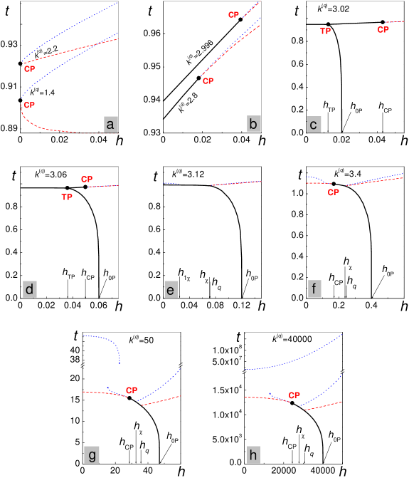
Figure 2: The $h$ vs $t$ phase diagrams at different values of quadrupolar interaction: a – $k^{(q)}=$1.4, 2.2; b – 2.8, 2.996; c – $k^{(q)}=3.02$; d – $k^{(q)}=3.06$; e – $k^{(q)}=3.12$; f – $k^{(q)}=3.4$; g – $k^{(q)}=50$; h – $k^{(q)}=40000$. Thick solid line indicates the first order temperature PT. Thin dashed and dotted lines correspond to the inflections in the temperature dependences of quadrupolar moment and to the maxima in the temperature dependences of static magnetic susceptibility, respectively. The special points are the triple point (TP), critical point (CP), and phase boundary point in the ground state (0P). $h_{1\chi}$, $h_{\chi}$ and $h_{q}$ are the coordinates of the intersection points of temperature PT line and of the lines, which correspond to maxima in $\chi(t)$ and to inflections in $q(t)$.

References

- (1) E.L. Nagaev, Magnetics with complicated exchange interaction, (Izd. Nauka, Moscow, 1988) (In Russian).
- (2) E. Čižmár, M. Kačmár, M. Orendáč, A. Orendáčová, J. Černák, A. Feher, J. Magn. Magn. Mater. 196-197, 433 (1999).
- (3) Th. Strässle, F. Juranyi, M. Schneider, S. Janssen, A. Furrer, K.W. Krämer, H.U. Güdel, Phys. Rev. Lett. 92, 257202 (2004).
- (4) H. Chen, P. Levy, Phys. Rev. B 7, 4267 (1973).
- (5) J. Sivardiere, M. Blume, Phys. Rev. B 5, 1126 (1972).
- (6) D.K. Ray, J. Sivardiere, Phys. Rev. B 18, 1401 (1978).
- (7) F.P. Onufrieva, I.P. Shapovalov, J. Moscow Phys. Soc. 1, 63 (1991).
- (8) H.A. Brown, Phys. Rev. B 31, 3118 (1985).
- (9) Yu.K. Rudavsky, O.Z. Vatamaniuk, V.P. Savenko, Condens. Matter Phys. (Lviv) iss. 5, 143 (1995).
- (10) O.Z. Vatamaniuk, Yu.K. Rudavsky, phys. stat. sol. (b) 197, 199 (1996).
- (11) J. Sivardiere, in Proc. Internat. Conf. Static critical phenomena in inhomogeneous systems, Karpacz 1984, Lecture notes in physics, 206 (Springer-Verlag, Berlin, 1984).
- (12) T. Iwashita, N. Uryû, phys. stat. sol. (b) 139, 597 (1987).
- (13) T. Iwashita, N. Uryû, phys. stat. sol. (b) 158, 347 (1990).
- (14) K. Takahashi, M. Tanaka, J. Phys. Soc. Japan 46, 1428 (1979).
- (15) S.I. Sorokov, R.R. Levitskii, O.R. Baran, Ukr. Fiz. Zhurn. 41, 490 (1996) (In Ukrainian).
- (16) K. Kasono, I. Ono, Z. Phys. B - Condensed Matter, 88, 205 (1992).
- (17) M. Blume, V.J. Emery, R.B. Griffiths, Phys. Rev. A 10, 1071 (1971).
- (18) D. Mukamel, M. Blume, Phys. Rev. A 10, 610 (1974).
- (19) D. Furman, S. Dattagupta, R.B. Griffiths, Phys. Rev. B 15, 441 (1977).
- (20) J. Bernasconi, F. Rys, Phys. Rev. B 4, 3045 (1971).
- (21) K.E. Newman, J.D. Dow, Phys. Rev. B 27, 7495 (1983).
- (22) K. Takahashi, M. Tanaka, J. Phys. Soc. Japan 48, 1423 (1980).
- (23) W. Hoston, A.N. Berker, Phys. Rev. Lett. 67, 1027 (1991).
- (24) R.R. Netz, A.N. Berker, Phys. Rev. B 47, 15019 (1993).
- (25) T. Balcerzak, M. Gzik-Szumiata, Phys. Rev. B 60, 9450 (1999).
- (26) M. Keskin, A. Erdinç, J. Magn. Magn. Mater. 283, 392 (2004).
- (27) O.R. Baran, R.R. Levitskii, phys. stat. sol. (b) 219, 357 (2000).
- (28) O.R. Baran, R.R. Levitskii, Phys. Rev. B 65, 172407 (2002).
- (29) O.F. de Alcantara Bonfim, C.H. Obcemea, Z. Phys. B - Condensed Matter 64, 469 (1986).
- (30) R.J.C. Booth, Lu Hua, J.W. Tucker, C.M. Care, I. Halliday, J. Magn. Magn. Mat. 128, 117 (1993).