Rethinking Atmospheric Turbulence Mitigation

Abstract

State-of-the-art atmospheric turbulence image restoration methods utilize standard image processing tools such as optical flow, lucky region and blind deconvolution to restore the images. While promising results have been reported over the past decade, many of the methods are agnostic to the physical model that generates the distortion. In this paper, we revisit the turbulence restoration problem by analyzing the reference frame generation and the blind deconvolution steps in a typical restoration pipeline. By leveraging tools in large deviation theory, we rigorously prove the minimum number of frames required to generate a reliable reference for both static and dynamic scenes. We discuss how a turbulence agnostic model can lead to potential flaws, and how to configure a simple spatial-temporal non-local weighted averaging method to generate references. For blind deconvolution, we present a new data-driven prior by analyzing the distributions of the point spread functions. We demonstrate how a simple prior can outperform state-of-the-art blind deconvolution methods.

I Introduction

I-A Motivation and Contributions

Atmospheric turbulence is one of the most devastating distortions in long-range imaging systems. Under anisoplanatic conditions, a scene viewed through turbulence is perturbed by random warping and blurring that are spatially and temporally varying. Their magnitudes and directions are influenced by temperature, distance and viewing angle [1]. Conventional turbulence restoration methods utilize standard image processing tools such as optical flow, lucky region fusion and blind deconvolution to recover images. While these methods are well-studied individually, they are agnostic to the physical model governing the turbulence. For example, the warping due to turbulence is not an arbitrary non-rigid deformation but the result of a wave propagating through layers of random phase screens.

The goal of this paper is to revisit the turbulence restoration pipeline by asking a question: If we rigorously follow the Kolmogorov’s model [2], how should each component in the turbulence restoration pipeline be configured so that the overall algorithm is grounded on physics. Our finding shows that when carefully designed, even very simple methods can perform better than sophisticated methods. See Figure 1 for a comparison between different turbulence image restoration methods applied to a static scene.

To elaborate on this main statement, in this paper we investigate two steps of the turbulence restoration pipeline:

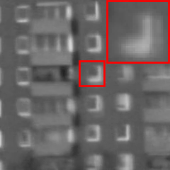
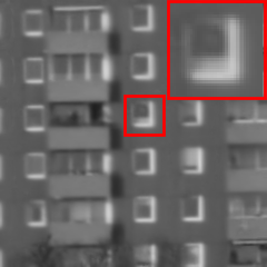
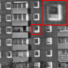
(a) Input	(b) Lucky Region	(c) Anan. et al. [3]
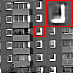
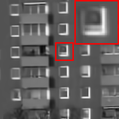
(d) Lou et al. [4]	(e) Zhu et al. [5]	(f) Ours

Figure 1: Comparison with state-of-the-arts on a real turbulence sequence Building. The proposed method is based on analyzing the physics of the turbulence.

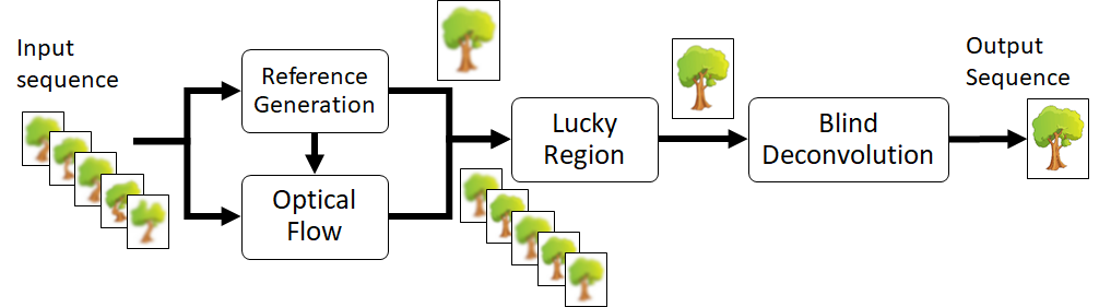
Figure 2: A typical turbulence restoration pipeline contains (i) reference frame generation, (ii) optical flow, (iii) lucky region fusion, and (iv) blind deconvolution. This paper focuses on the reference frame generation and the blind deconvolution steps.

• Reference Frame. Majority of the turbulence restoration pipelines involve optical flow and lucky region fusion. Both steps require a good reference, and typically the reference is computed from its neighboring frames. The number of frames plays a critical role here. If we use too few frames, then the turbulence pixels are not stabilized. However, if we use too many frames, then the image will be over-smoothed. Typically, the number of frames is unknown ahead of the restoration, and is tuned manually by the user. More sophisticated methods have built-in iterative mechanisms to update the reference while recovering the image, but these methods are time consuming.

  We study the reference frame generation problem from a physics point of view. Using a simplified Kolmogorov turbulence model, we assume that the turbulence point spread function is a kernel with random spatial offsets. By leveraging tools in high dimensional probability, in particular the large deviation theory, we rigorously analyze the number of adjacent frames required to produce a reasonable reference frame. Our theoretical results reveal potential flaws that could happen if we ignore the physics. (See Section 2.)

• Blind Deconvolution. Blind deconvolution is used to remove the diffraction limited blur after the lucky region fusion step. Normally, at this stage one would assume that the blur is spatially invariant and so any off-the-shelf blind deconvolution method can be applied (e.g., deep neural network). However, rather than treating the blur as a completely unknown quantity, we argue that the diffraction limited blur in turbulence has a unique prior which can offer a good solution. We articulate the problem by building an accurate turbulence simulator (via wave propagation equations) to generate short exposure point spread functions, and learn the basis functions as well as the prior distribution. We show that a very simple Bayesian estimation is sufficient to provide high quality results. (See Section 3.)

I-B Related Work

Turbulence image restoration is a well studied subject. The focus of this paper is the image processing approach. The underlying assumption is that the imaging system is passively acquiring images where the light source is incoherent. We do not use coherent light sources to illuminate the object and use adaptive optics to compensate for the phase shifts. Readers interested in active imaging approaches can consult, e.g., [6].

The image processing literature on turbulence is rich. In general, most of the methods follow a similar pattern: Reference frame, optical flow, lucky region, and deconvolution, as shown in Figure 2. In the followings we briefly describe a few better known methods.

• Methods for Static Scenes. Most of the turbulence image restoration methods in the literature are designed for static scenes, i.e., both the object and the background are not moving. Because the scene is static, all pixel movements are caused by turbulence. Therefore, one of the simplest approaches to generate a reliable reference frame is to take the temporal average. This has been used in many previous work, e.g., Lou et al. [4], Zhu and Milanfar [5], Gilles and Osher [7], and more recently Hardie et al. [8] and Lau et al. [9].

  Once the reference frame is generated, it will be sent to an optical flow to estimate the motion. Depending on the complexity of the scene and the computing budget, optical flow can be as simple as the traditional block matching by Hardie et al. [8] or more customized methods such as B-spline by Zhu and Milanfar [5], or feature matching by Anantrasirichai et al. [3].

  The output of the optical flow is a sequence of motion compensated frames. If the scene is static, these processed frames are aligned but the blur is spatially varying. The purpose of the lucky region fusion is to pick the sharp regions to form a so called “lucky frame”. The way to determine the lucky region is very similar to the reference frame. Instead of using the temporal average, there is a term measuring the magnitude of the gradient [4, 3]. Sharper frames typically have stronger gradients.

  The final step of the pipeline (Figure 2) is the blind deconvolution. In principle, the image sent to this stage should have been recovered except the diffraction limited blur. The goal of blind deconvolution is to remove the remaining blur. Since blind deconvolution is a generic problem, many methods can be used, e.g., Wiener filtering by Hardie et al. [8] or minimizing energy functions such as total variation as in [4, 7, 5].

• Methods for Dynamic Scenes. Methods for dynamic scenes (moving foreground and a static background) have more variations. For example, instead of using the lucky region fusion, Gilles and Osher [7] proposed to use wavelet burst accumulation to boost high frequency components. For large moving objects, Nieuwenhuizen et al. [10] proposed to use a super resolution fusion step to ensure spatial consistency, and Huebner [11] proposed a block matching algorithm and local image stacking.

  Because of the moving foreground, one alternative approach is to use advanced segmentation algorithms to extract the foreground. The background can then be recovered using the static scene methods. Several papers are based on this idea, e.g., Oreifej et al. [12], Halder et al. [13] and Anantrasirichai et al. [14]. However, a fundamental issue of segmentation-based methods is that in the presence of turbulence distortion, the object boundaries are very difficult to determine. Thus, artifacts are easily generated by these methods.

• Other Methods. Beyond the above “mainstream” methods, there are also customized approaches for specific context, e.g., underwater imaging using deep learning [15], among a few others, e.g., bispectral analysis [16], infra-red [17], face recognition in turbulence [18], and holographic systems [19].

In this paper, we focus on the pipeline shown in Figure 2 because it is the most common pipeline which can be applied to both static and dynamic scenes. Among the components of the pipeline, we are particularly interested in the reference generation and the blind deconvolution step. The optical flow and the lucky region fusion are based on existing implementations. For example, for optical flow we use [20], and for lucky region fusion we use a modified version of [21].

II Reference Frame

We first look at reference frame generation. The objective of this section is to present a simple and generic method. The idea is based on spatial-temporal non-local weighted averaging. After presenting the method, we will rigorously analyze the number of adjacent frames required for the averaging. We will show a few non-trivial results based on large deviation theory.

To keep our notation simple, we consider only one dimension in space. Extension to two dimensions is straight forward.

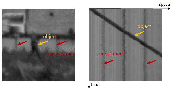
Figure 3: Space-time plot of a moving scene. The moving object will cause a significant displacement in the space-time plot. However, turbulence only perturbs a pixel by vibrating them around the center positions.

II-A Non-local Reference Generation Method

The motivation of our reference generation method is illustrated in Figure 3, where we show a space-time plot of a typical turbulence distorted sequence. The moving object and a static pattern demonstrate very different trajectories: The moving object shows clear movement across the space, whereas a static pattern only vibrates at its center location. This difference suggests that if we pick a local patch distorted by turbulence, we should be able to find a similar patch in a small spatial-temporal neighborhood. In contrast, it will be more difficult to find a match for a motion patch.

Let $\boldsymbol{y}_{t}\in\mathbb{R}^{N}$ be the $t$-th frame of the input video. Let $\boldsymbol{y}_{i,t}\in\mathbb{R}^{d}$ be a $d$-dimensional patch located at pixel $i$. We set up a spatial-temporal search window of size $L\times T$, and then compute the distance between the current patch $\boldsymbol{y}_{0,0}\in\mathbb{R}^{d}$ and all other patches $\{\boldsymbol{y}_{i,t}\;|\;i\in\Omega_{L},\;t\in\Omega_{T}\}$ within the search window. This gives us

$$\Delta_{i,t}=\|\boldsymbol{y}_{i,t}-\boldsymbol{y}_{0,0}\|^{2},$$ (1)

where $i\in\Omega_{L}\overset{\text{def}}{=}\{1,\ldots,L\}$ and $t\in\Omega_{T}\overset{\text{def}}{=}\{1,\ldots,T\}$. Intuitively, we can think of $\Delta_{i,t}$ as a measure of how similar $\boldsymbol{y}_{i,t}$ is to $\boldsymbol{y}_{0,0}$. If $\boldsymbol{y}_{0,0}$ is distorted by turbulence, then at least one of these $L$ patches in the adjacent frame should be similar to $\boldsymbol{y}_{0,0}$. If $\boldsymbol{y}_{0,0}$ is a moving object, then no patch in the window will be similar to $\boldsymbol{y}_{0,0}$. See Figure 4 for a pictorial illustration. Thus, for every frame, we can check the smallest residue among the spatial neighborhood, and define the temporal weight as

$$w_{t}=\exp\left\{-\beta\min_{i\in\Omega_{L}}\left\{\Delta_{i,t}\right\}\right\}.$$ (2)

Then, we use $w_{t}$ to compute the reference patch via

$$\boldsymbol{\widehat{y}}_{0,0}=\frac{\sum_{t\in\Omega_{T}}w_{t}\boldsymbol{y}_{0,t}}{\sum_{t\in\Omega_{T}}w_{t}}.$$ (3)

Note that $\boldsymbol{\widehat{y}}_{0,0}$ overlaps when we move to another patch of the image. The overlapping can be taken care of by averaging out the overlapping pixels.

We emphasize that (3) is an extremely simple operation. It does not require object segmentation such as [12, 13, 14], and yet it is applicable to both static and dynamic scenes.

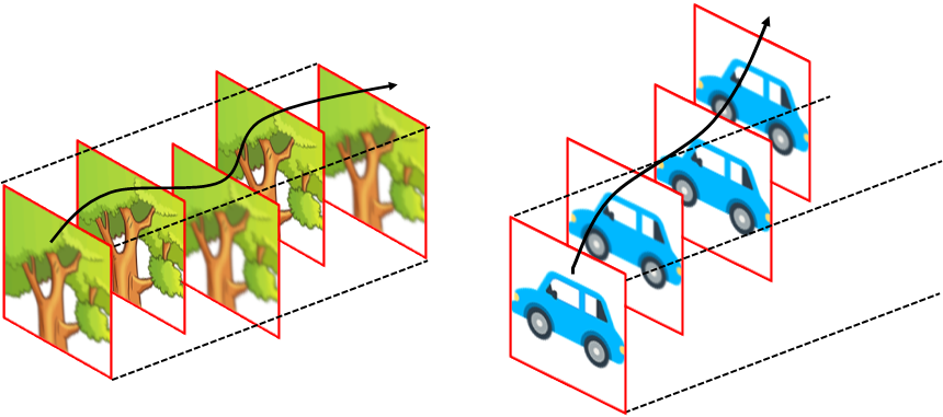
Figure 4: Given a current patch, the proposed reference frame generation method computes a weighted average across the adjacent frames. [Left] Turbulence: We average every patch along the time axis. [Right] Motion: We put small weights to patches that stays far from the center.

II-B Empirical Plot of $\beta$ for Static Scenes

Like any other non-local averaging method, the hyper-parameter $\beta$ in (2) plays a critical role: If $\beta$ is too large, then we are dropping most of the adjacent frames, hence the result is reliant on $\boldsymbol{y}_{0,0}$. If $\beta$ is too small, then we are being over-inclusive. In principle, $\beta$ should be chosen according to the turbulence. We now discuss how.

In Kolmogorov’s model, turbulence is characterized by the refractive-index structure parameter $C_{n}^{2}$. $C_{n}^{2}$ is a function of the temperature, wavelengths and distance [8]. Integrating $C_{n}^{2}$ over the wave propagation path will give us the Fried parameter $r_{0}$. The reciprocal of $r_{0}$ normalized by the aperture diameter $D$ is a quantity $D/r_{0}$ we typically see in the literature. Larger $D/r_{0}$ means stronger turbulence [1].

To initiate the discussion let us look at Figure 5. The figure shows an empirical plot of the best $\beta$ as a function of $D/r_{0}$ for a static point source. We generate this plot by simulating how the point source goes through the turbulence media for a specific $D/r_{0}$ ratio (see Appendix for details of our simulator). We then pick the largest $\beta$ that makes $\|\boldsymbol{z}_{0}-\widehat{\boldsymbol{y}}_{0}\|^{2}\leq\epsilon$ for some tolerance level $\epsilon$, where $\boldsymbol{z}_{0}$ is the ground truth and $\widehat{\boldsymbol{y}}_{0}$ is the estimated reference point source. The experiment is repeated 10 times to average out the randomness of the individual turbulence. We report the mean and the standard deviation.

Figure 5 matches with our intuitions: As turbulence becomes stronger (larger $D/r_{0}$), we require more frames to average out the randomness (hence $\beta$ drops). But what is the exact relationship between the turbulence strength and the number of frames? In addition, why does $\beta$ stay at a constant when $D/r_{0}<1$?

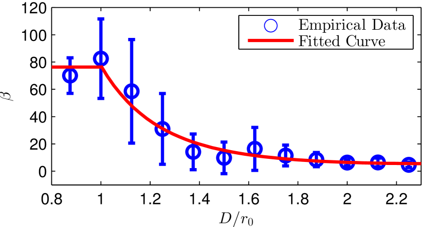
Figure 5: The optimal $\beta$ as a function of the turbulence strength $\frac{D}{r_{0}}$. The circles are the average of 10 independent trials and the error bar denotes one standard deviation.

II-C Short and Long Exposure PSFs

To understand the behavior of $\beta$, we recall an old result by Fried [22] showing that 90% of the disturbance due to turbulence is attributed to the random shifting of the points spread function (PSF). What this suggests is a simple model for the PSF by writing it as $h(x-\Theta)$, where $h(\cdot)$ is a fixed kernel and $\Theta$ is a random variable drawn from some distribution $p_{\Theta}(\theta)$. Therefore, given a fixed shape of the PSF $h(\cdot)$, we can shift it spatially to obtain an instantaneous PSF. The fluctuation of the shift is determined by $p_{\Theta}(\theta)$.

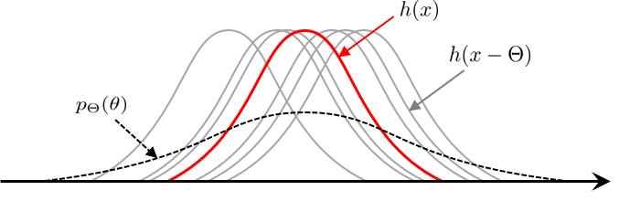
Figure 6: A simplified model of the PSF by shifting $h(x)$ using a random offset. The distribution of $\Theta$ is given by $p_{\Theta}(\theta)$.

In turbulence terminology, the un-perturbed PSF $h(\cdot)$ is called a short-exposure PSF (short-PSF) [1]. For mathematical analysis we assume that $h(\cdot)$ is a smoothing kernel with some parameter $\nu$.

Definition 1.

The point spread function (PSF) $h(\cdot)$ takes the form of

$$h_{\nu}(x)=\frac{1}{\nu}K\left(\frac{x}{\nu}\right)$$ (4)

for some smoothing kernel $K$, and some constant $\nu>0$.

In this definition, the number $\nu$ controls the “bandwidth” of $h_{\nu}$ without changing its “volume”. The expectation $\mathbb{E}_{\Theta}[h_{\nu}(x-\Theta)]$ is called the long-exposure PSF (long-PSF). The long-PSF can be shown as the convolution of the short-PSF and the distribution $p_{\Theta}(\theta)$:

$$\begin{split}\mathbb{E}_{\Theta}[h_{\nu}(x-\Theta)]&=\int h_{\nu}(x-\theta)p(\theta)d\theta\\ &=(h_{\nu}\circledast p_{\Theta})(x).\end{split}$$ (5)

To analyze the practical situation, we also define a finite sample estimate

$$\widetilde{h}_{\nu}(x)\overset{\text{def}}{=}\frac{1}{T}\sum_{t=1}^{T}h_{\nu}(x-\theta_{t}),$$ (6)

where $\{\theta_{t}\}$ are i.i.d. copies of $\Theta$. Our goal is to analyze how $T$ changes with $\mathrm{Var}[\Theta]$, as $T$ is a proxy for $\beta$ and $\mathrm{Var}[\Theta]$ is a proxy for $D/r_{0}$.

Remark: What is the distribution $p_{\Theta}(\theta)$? If we look at how the short exposure and the long exposure PSFs are derived in the literature, we can see that the distribution is in fact a Gaussian. See Roggemann [1] (Section 3.5). In particular, take the ratio of the long exposure PSF in Equation 3.125 and the short exposure PSF Equation 3.135. Because of this, we model the distribution $p_{\Theta}(\theta)$ as a Gaussian with zero mean and variance $\sigma^{2}$: $\Theta\sim\mathcal{N}(0,\sigma^{2})$.

II-D Concentration of Measure Results

We now present the main theoretical result. The following theorem shows that, as $T$ increases, the finite sample estimate $\widetilde{h}_{\nu}(x)$ will approach its expectation $(h_{\nu}\circledast p_{\Theta})(x)$ with high probability.

Theorem 1.

(Concentration of $\widetilde{h}_{\nu}(x)$). For any $\epsilon>0$,

$$\sup_{x\in\mathbb{R}}\;\mathbb{P}\left(\left|\widetilde{h}_{\nu}(x)-(h_{\nu}\circledast p_{\Theta})(x)\right|>\epsilon\right)\leq$$ (7)

$$\quad\quad 2\exp\left\{-\frac{\epsilon^{2}T}{2\sup\limits_{x\in\mathbb{R}}V_{\nu}(x,\sigma)+2\nu^{-1}M\epsilon/3}\right\}\overset{\text{def}}{=}\alpha,$$

where $M$ is an upper bound of $K(\cdot)$, i.e., $0\leq K(x)\leq M$ for all $x\in\mathbb{R}$, and $V_{\nu}(x,\sigma)\overset{\text{def}}{=}\mathrm{Var}[h_{\nu}(x-\Theta)]$.

Proof.

See Appendix for proof. ∎

There are several important implications of the theorem:

• Fix $\epsilon$. As number of frames $T$ increases, the probability of getting a large deviation is exponentially decaying. In terms of turbulence, it says that the finite sample PSF converges to the long-PSF, something we expect and something well-known.

• While $T$ can be arbitrarily large, in practice we always use the smallest $T$ such that the probability meets the tolerance upper bound $\alpha$. This is coherent with how $\beta$ is generated in Figure 5.

• The smallest $T$ is determined by $V_{\nu}(x,\sigma)$. As the turbulence becomes stronger, $V_{\nu}(x,\sigma)$ increases. The theorem then predicts that we need a large $T$ to achieve a tolerance $\alpha$. This is precisely what is happening in Figure 5 for $D/r_{0}\geq 1$: the stronger turbulence we have, the more frames we need.

• A big surprise comes when we compute the variance:

  $$V_{\nu}(x,\sigma)= \mathrm{Var}_{\Theta}[h_{\nu}(x-\Theta)]$$

  $$= \mathbb{E}_{\Theta}[h_{\nu}^{2}(x-\Theta)]-\mathbb{E}_{\Theta}[h_{\nu}(x-\Theta)]^{2}$$

  $$= (h_{\nu}^{2}\circledast p_{\Theta})(x)-(h_{\nu}\circledast p_{\Theta})^{2}(x).$$

  If we plot $\sup_{x\in\mathbb{R}}V_{\nu}(x,\sigma)$ as a function of $\sigma$ (i.e., $\sqrt{\mathrm{Var}[\Theta]}$), we obtain Figure 7. As the turbulence strength $\sigma$ increases, $\sup_{x\in\mathbb{R}}V_{\nu}(x,\sigma)$ rises and then drops! In other words, the theorem predicts that when turbulence is extremely strong, we actually need very few frames. This is counter intuitive.

• More problematically, the existence of a maximum of $\sup_{x\in\mathbb{R}}V_{\nu}(x,\sigma)$ is guaranteed for any PSF $h_{\nu}(\cdot)$. See Theorem 2 below. Therefore, the problem is universal.

Theorem 2.

If $h_{\nu}$ is Lipschitz continuous on $\mathbb{R}$, or continuous but with compact support on $\mathbb{R}$, then $\sup_{x\in\mathbb{R}}V_{\nu}(x,\sigma)$, as a function of $\sigma$, attains a global maximum on $(0,\infty)$.

Proof.

The proof requires setting up several preliminary results in real analysis. We outline a sketch of the proof in the Appendix. Readers interested in the complete proof can check the Supplementary material. ∎

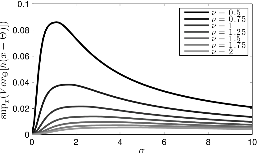
Figure 7: $\sup_{x\in\mathbb{R}}V_{\nu}(x,\sigma)$ vs. $\sigma$. The smoothing kernel $K$ is taken to be the standard Gaussian function here. The existence of a peak suggests that the blur and shift of a turbulence have to be increase simultaneously, or otherwise the result will be physically invalid.

So what causes the disparity between our intuition and the theorem? The theorem is perfectly fine. What is not correct is a false assumption we overlooked. In the real turbulence setting, $\mathrm{Var}[\Theta]$ (i.e., $\sigma$) cannot be arbitrarily large. More specifically, the allowable shift $\sigma$ for any real turbulence must be bounded by the bandwidth $\nu$ of the PSF. When $\sigma$ is bounded, we can show that $\sup_{x\in\mathbb{R}}V_{\nu}(x,\sigma)$ only operates in the increasing regime before reaching the maximum. Proposition 1 below shows a special case where $K$ is a boxcar kernel (so that we can derive analytic solution.)

Proposition 1.

If $K$ is the boxcar kernel, then for $\sigma\leq\left(\Phi^{-1}\left(\frac{3}{4}\right)\right)^{-1}\nu\approx 1.48\nu$, $V_{\nu}(x=0,\sigma)$ is an increasing function in $\sigma$, where $\Phi(\cdot)$ is the normal CDF.

Proof.

See the Appendix for proof. ∎

The implication of Proposition 1 is significant. It suggests that many warping models based on the ad-hoc non-rigid deformations could be flawed if not modeled properly. A realistic turbulence must have shift and blur happening at the same time. A crude approximation of the shift with respect to the blur is $\sigma\approx 1.48\nu$. An empirical plot of this result is shown in Figure 8.

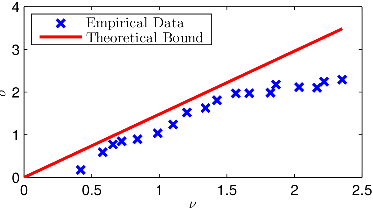
Figure 8: Verification of Proposition 1. The empirical data are generated by first simulating a PSF and measuring the bandwidth $\nu$ and the shift $\sigma$. The empirical data matches with the theory which predicts that $\sigma\leq 1.48\nu$.

Remark. The results in Proposition 1 can be improved by assuming a Gaussian kernel instead of the boxcar kernel. However, to do so we need to use numerical methods because the Gaussian kernel does not allow closed-form analysis.

II-E The Weak Turbulence Case

We now consider $\beta$ when $D/r_{0}<1$. In this regime, the random shifting caused by the turbulence is insignificant compared to the diffraction limit of the PSF. In the turbulence literature, this phenomenon is known as that the “seeing error” due to the turbulence effects being overridden by the Airy disc [6]. Putting in our terminology, we can say that $\mathrm{Var}[\Theta]\approx 0$ and so $h_{\nu}(x-\Theta)\approx h_{\nu}(x)$.

When $h_{\nu}(x-\Theta)\approx h_{\nu}(x)$, the random shifting is negligible. Thus, we can use any number of frames, including just one frame or many frames. The numerical result in Figure 5 shows that $\beta$ is at the maximum (i.e., as few frames as possible.) However, a different choice of $\beta$ will perform equally well.

II-F Moving Objects

In the presence of motion, the short-PSF changes from $h_{\nu}(x-\Theta)$ to $h_{\nu}(x(t)-\Theta)$, where $x$ is now a function of time. Assuming constant velocity so that $x^{\prime}(t)=c$ for some $c\in\mathbb{R}$, we can show that

$$\mathbb{E}\left[\frac{1}{T}\sum_{t=1}^{T}h(x+ct-\Theta)\right]$$

$$\approx\mathbb{E}\left[\frac{1}{T}\sum_{t=1}^{T}\Big{\{}h(x-\Theta)+h^{\prime}(x-\Theta)ct\Big{\}}\right]$$

$$=\underset{\mbox{turbulence}}{\underbrace{(h_{\nu}\circledast p_{\Theta})(x)}}+\underset{\mbox{motion}}{\underbrace{\frac{c(T+1)}{2}(h_{\nu}^{\prime}\circledast p_{\Theta})(x)}}.$$ (8)

Therefore, the perturbation caused by motion is captured by the bias $\frac{c(T+1)}{2}(h_{\nu}^{\prime}\circledast p_{\Theta})(x)$. If we assume that $|(h_{\nu}^{\prime}\circledast p_{\Theta})(x)|\leq R$ for all $x$, then

$$\begin{split}\frac{c(T+1)}{2}(h_{\nu}^{\prime}\circledast p_{\Theta})(x)&\leq B\\ \;\;\;\Longleftrightarrow\;\;\;T&\leq\frac{2B}{cR}-1.\end{split}$$ (9)

The right hand side of (9) provides an upper bound on $T$. Let us differentiate the $T$’s for static and dynamic case. We denote the number of frames for the static case as $T_{\mathrm{s}}$, and that for dynamic case as $T_{\mathrm{d}}$. The overall $T$ is the smaller of the two: $T=\min\{T_{\mathrm{s}},T_{\mathrm{d}}\}$.

Now we can comment on the implication of (9). When $c=0$, i.e., static scene, we have $T_{\mathrm{d}}<\infty$. In this case, the actual number of frames $T$ is determined by the turbulence $T_{\mathrm{s}}$. When the velocity $c$ grows, $T_{\mathrm{d}}$ drops. If $T_{\mathrm{d}}$ drops below $T_{\mathrm{s}}$, then $T=T_{\mathrm{d}}$. Thus for very fast moving objects, the number of frames is limited by $T_{\mathrm{d}}$.

In terms of our algorithm, the factor $\frac{2B}{R}$ serves the role of the spatial search window size $L$. If $L$ is small, then even patches with small motion will be skipped. This shows the two distinctive roles of $\beta$ and $L$. $\beta$ is used to measure the turbulence, whereas $L$ is used to measure the object velocity. The typical range of $\beta$ is given by Figure 5, and the typical value of $L$ is $11\times 11$ for a $500\times 500$ image.

III Blind Deconvolution

In this section we look at the blind deconvolution step. Our basic argument is that the blind deconvolution for a turbulence problem does not need to be very complicated because the turbulence PSF is well structured. Our goal is to exploit this structure and to propose a simple but effective blind deconvolution method.

III-A Blind Deconvolution Algorithm

Recall that the blind deconvolution is applied to the output of the lucky region fusion step. We need a blind deconvolution because we do not know the blur and the latent image.

The proposed algorithm begins with a standard alternating minimization:

$$\boldsymbol{z}^{k+1} =\mathop{\underset{\boldsymbol{z}}{\mbox{argmin}}}\;\|\boldsymbol{y}-\boldsymbol{h}^{k}\circledast\boldsymbol{z}\|^{2}+\lambda g(\boldsymbol{z})$$ (10)

$$\boldsymbol{h}^{k+1} =\mathop{\underset{\boldsymbol{h}}{\mbox{argmin}}}\;\|\boldsymbol{y}-\boldsymbol{h}\circledast\boldsymbol{z}^{k+1}\|^{2}+\gamma r(\boldsymbol{h}),$$ (11)

where $\boldsymbol{y}$ is the output of the lucky region fusion, $\boldsymbol{h}$ is the unknown PSF, and $\boldsymbol{z}$ is the latent clean image. The equation for $\boldsymbol{z}^{k+1}$ is to update the latent image $\boldsymbol{z}$ by using the currently estimated PSF $\boldsymbol{h}^{k}$. Similarly, the equation for $\boldsymbol{h}^{k+1}$ is to update the PSF by using the currently estimated $\boldsymbol{z}^{k+1}$. In these two equations, $g(\cdot)$ and $r(\cdot)$ are regularization functions for $\boldsymbol{z}$ and $\boldsymbol{h}$, respectively. For performance, $g(\cdot)$ is chosen as the Plug-and-Play prior [23] using BM3D as the denoiser.

At the output of the lucky region fusion step, only the sharpest frames are aggregated to form a diffraction limited image [5]. Thus, the PSF for the blind deconvolution step is a short-PSF plus minor distortions in phase and magnitude (due to uncertainty caused by finite sample averaging and optical flow). To encapsulate the features of these distorted short-PSFs, we adopt a simple linear model by writing $\boldsymbol{h}$ as a set of basis vectors $\boldsymbol{h}=\sum_{i=1}^{m}w_{i}\boldsymbol{u}_{i}$, where $\{\boldsymbol{u}_{i}\}_{i=1}^{m}$ are to be trained. By incorporating this into the algorithm, we replace (11) by two steps:

$$\boldsymbol{w}^{k+1} =\mathop{\underset{\boldsymbol{w}}{\mbox{argmin}}}\;\left\|\boldsymbol{y}-\left(\sum_{i=1}^{m}w_{i}\boldsymbol{u}_{i}\right)\circledast\boldsymbol{z}^{k}\right\|^{2}+\gamma r(\boldsymbol{w})$$ (12)

$$\boldsymbol{h}^{k+1} =\sum_{i=1}^{p}w_{i}^{k+1}\boldsymbol{u}_{i},$$ (13)

where $r(\boldsymbol{w})$ is a regularization function on $\boldsymbol{w}$. The overall blind deconvolution algorithm now consists of three steps: updating the image estimate (10), followed by estimating the weight (12) and constructing the PSF estimate (13). The algorithm repeats until convergence. Like the reference generation step, we emphasize that the proposed blind deconvolution method is extremely simple. However, we will show that by carefully choosing $\{\boldsymbol{u}_{i}\}_{i=1}^{m}$ and $r(\boldsymbol{w})$, this method is sufficient to produce good results.

III-B Basis Functions

Given that we are working on turbulence, one straight-forward approach to construct the basis functions is to simulate a large number of training PSFs and learn the principal components. To this end, we simulate 40,000 short-PSFs, each of size $15\times 15$. These 40K short-PSFs cover a wide range of $C_{n}^{2}$ from $5\times 10^{-17}$ to $5\times 10^{-16}$, which is sufficient to model mild to medium turbulence. After generating these training samples we learn the principal components using the standard PCA.

Figure 9 shows a few snapshots of the generated short-PSFs at $C_{n}^{2}=10^{-17}$. We see that in general the short-PSFs are highly structured. All PSF shown have a similar mean and small distortions around the center. If we look at the basis functions, we see that the basis functions are nothing but a set of directional filters. These directional filters are orthogonal.

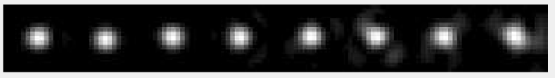
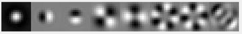
Figure 9: [Top] Simulated short-PSFs, displayed according to increasing turbulence level from left to right. [Bottom] The first 8 principle components.

III-C Prior Distribution of the Weights

Once the bases $\{\boldsymbol{u}_{1},\ldots,\boldsymbol{u}_{m}\}$ are defined, we can examine the weight $\boldsymbol{w}=[w_{1},\ldots,w_{m}]^{T}$. To this end, we conduct an experiment to approximate a simulated short-PSF using as few bases as possible. This leads to an $\ell_{0}$ optimization by minimizing the number of active bases while bounding the error by $\tau$:

$$\widehat{\boldsymbol{w}}=\mathop{\underset{\boldsymbol{w}}{\mbox{argmin}}}\;\;\|\boldsymbol{w}\|_{0}\;\;\mbox{s.t.}\;\;\left\|\boldsymbol{h}_{\mathrm{sim}}-\sum_{i=1}^{m}w_{i}\boldsymbol{u}_{i}\right\|^{2}\leq\tau.$$ (14)

Here, $\boldsymbol{h}_{\mathrm{sim}}$ denotes a simulated training short-PSF. We repeat the experiment for 100,000 different $\boldsymbol{h}_{\mathrm{sim}}$, and we plot the histogram of each weight $\widehat{w}_{i}$ over these 100,000 trials. The empirical histogram is shown in Figure 10.

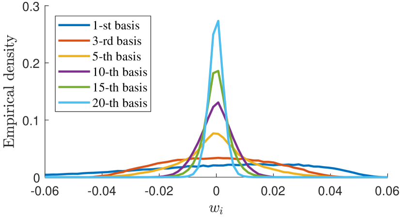
Figure 10: Empirical distributions of the weights by solving (14) with 100,000 different simulated PSF $\boldsymbol{h}_{\mathrm{sim}}$. The empirical distribution demonstrates a double-sided exponential distribution.

By inspecting the histograms in Figure 10, we notice a double-sided exponential distribution. This suggests a product of exponential distributions for $\boldsymbol{w}$:

$$p(\boldsymbol{w})=\exp\left\{-\sum_{i=1}^{m}\frac{|w_{i}|}{d_{i}}\right\},$$ (15)

where $d_{i}$ measures the standard deviation of the individual exponential. Consequently we can define the regularization by taking the negative log: $r(\boldsymbol{w})=\sum_{i=1}^{m}\frac{|w_{i}|}{d_{i}}$.

IV Experimental Results

IV-A Ablation Study of Reference Generation

We first consider an ablation study of the reference generation method. To allow quantitative comparison, we simulate a 100-frame static-scene turbulence-distorted sequence at several different $C_{n}^{2}$’s. We use two metrics in this experiment. The first metric is the PSNR between the generated reference and the ideal short-exposure image. The ideal short-exposure image is generated by filtering the image with a short-PSF. This short-PSF is obtained by centroiding and averaging the simulated PSFs. The second metric is the PSNR between the final restoration result and the ground truth. That is, we fix the components of the pipeline except the reference generation step. The goal is to test the influence of the reference image.

The results of this experiment are shown in Table I. The first half of the table shows that the proposed reference generation method produces a reference that is closer to the ideal short-exposure image than the conventional temporal averaging. Figure 11 shows a visual comparison. The second half of the table shows that the influence of the reference frame is significant especially for large $C_{n}^{2}$. One reason is that as $C_{n}^{2}$ grows, the turbulence distortion becomes stronger and so the reference is over-smoothed. Feeding this over-smoothed reference to optical flow and lucky frame will degrade the performance significantly.

$C_{n}^{2}$ ($\times 10^{-17}$)	$5$	$8$	$20$	$50$
(PSNR between reference and ideal short exposure)
Tmp Avg	39.82	38.67	33.48	28.57
Ours	40.23	39.60	35.85	31.26
(Overall PSNR by changing reference in the pipeline)
Tmp Avg	27.72	27.47	25.79	23.69
Ours	27.77	27.67	27.29	26.47

TABLE I: [Top] Comparing reference with respect to the ideal short exposure image. [Bottom] Ablation study by changing the reference in the pipeline.

In addition to the synthetic experiment, we also test on real moving sequences shown in Figure 12. As the person in the sequence moves, temporal averaging will blur out the person. In contrast, the proposed method can retain the person while stabilizing the background.

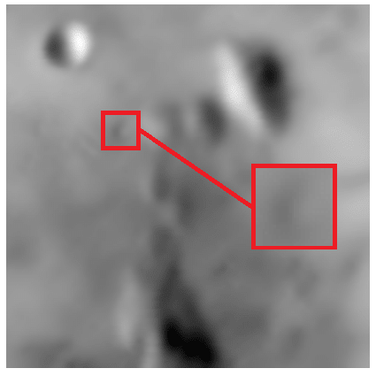
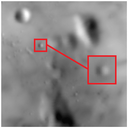
Ideal Short Exp.	Tmp Avg	Ours

Figure 11: Synthetic experiment by simulating turbulence distorted images. This figure compares the generated reference with respect to the ideal short exposure image.

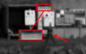
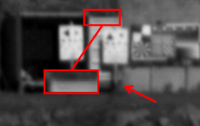
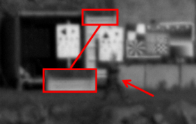
(a) Raw input	(b) Tmp Avg	(c) Ours

Figure 12: [Left] Raw input. [Middle] Temporal averaging: The man is blurred over 100 frames. [Right] Ours: The man remains in the image while the background is stabilized.

IV-B Ablation Study of Blind Deconvolution

The second experiment is an ablation study to test the effectiveness of the blind deconvolution algorithm. The competing methods we consider include a classical method by Shan et al. [24], and two very recent deep neural networks by Chakrabarti [26] and Xu et al. [25]. We downloaded the original implementations of these methods and used the pre-trained models. Internal parameters (for [24]) are fined tuned to maximize the performance. For our proposed method, we fix $\lambda=0.05$ and $\gamma=1\times 10^{-4}$ for all experiments reported in this paper.

We use the 24 images in the Kodak image dataset for experiment. Every image is blurred with 50 random short-PSFs under 5 different turbulence levels with $C_{n}^{2}$ from $5\times 10^{-17}$ to $5\times 10^{-16}$. Thus each method at every turbulence level consists of 1200 testing scenarios. Since this is a simulated experiment, we have access to the ground truths to compute the PSNR values. The average PSNR over the 50 random PSFs are shown in Table II.

For visual quality comparison, we demonstrate a result with the USAF resolution chart using turbulence at a level of $C_{n}^{2}=2.5\times 10^{-16}$. It can be seen in Figure 13 that the result using our method contains the least amount of artifacts. The estimated PSF is also more structured and interpretable than the deep neural networks [26, 25].

$C_{n}^{2}$ ($\times 10^{-17}$)	$5$	$15$	$25$	$35$	$45$
Shan et al. [24]	27.25	26.52	26.59	25.91	23.89
Chakrabarti [26]	27.32	26.69	26.31	24.80	24.49
Xu et al. [25]	26.68	26.08	26.04	24.45	24.21
Ours	27.69	27.02	27.00	26.24	24.58

TABLE II: Ablation study of blind deconvolution algorithms. The PSNRs are averaged over 24 images of the Kodak image dataset, and every image is tested 50 times for different random short-PSFs. Thus every data point reported in this table is an average over 1200 testing scenarios.

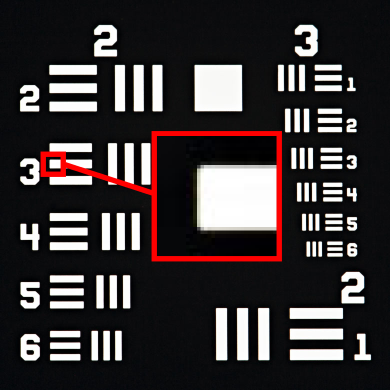
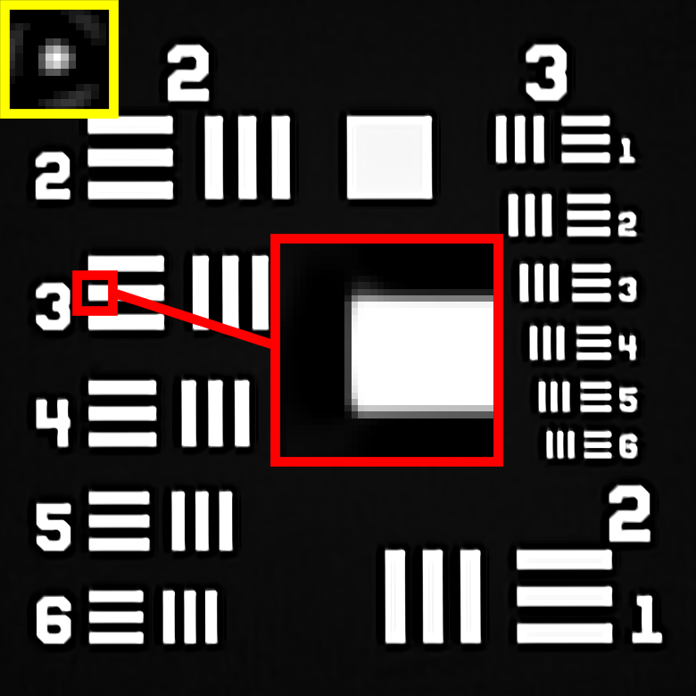
(a) Ground Truth	(b) Lucky Region	(c) Ours: 24.78 dB
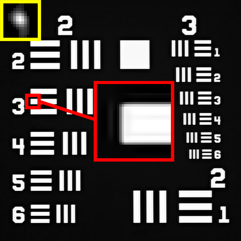
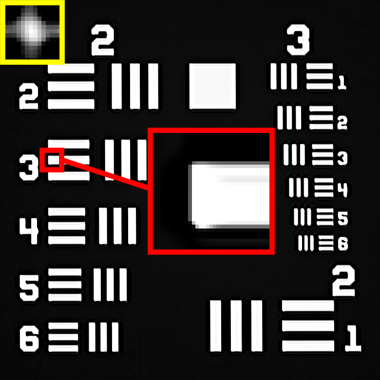
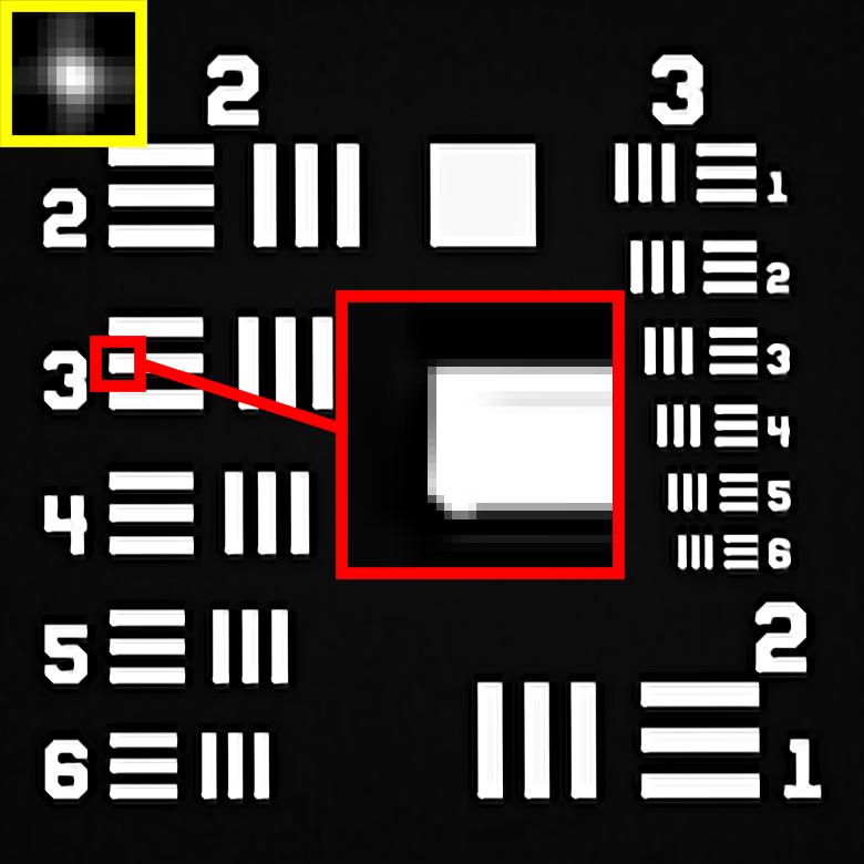
(d) [24]: 23.34 dB	(e) [26]: 22.99 dB	(f) [25]: 23.75 dB

Figure 13: Experiments with USAF resolution chart. Corresponding PSFs are shown in the uppper-left corner. Zoom in for better view.

IV-C Overall Algorithm on Real Data

The third experiment is to compare the proposed pipeline with other turbulence restoration methods. Since we have reported simulated results in the previous two subsections, here we report performance on real data.

The first two sets of comparisons are the Building in Figure 1 and the Chimney in Figure 14 [27]. We compare with three methods: Sobolev gradient flow by Lou et al. [4], B-spline + deblurring by Zhu and Milanfar [5], and a wavelet enhancement method by Anantrasirichai et al. [3]. The implementation of the methods are provided by the original authors, and the internal parameters are tuned according to the best of our knowledge. There are a few other methods discussed in the introduction, but we were not able to obtain the reproducible source codes.

The next two sets of comparison are the Man sequence as shown in Figure 14, and the Car sequence as shown in Figure 16. The walking man’s motion is highly horizontal, hence it is easily “washed out” by existing methods. In contrast, the proposed method is able to preserve the man and generate a reliable reference. The car sequence is a considerably harder problem, as the car is moving towards the viewer. The proposed method, however, is able to stabilize the background fences while sharpens the licence plate.

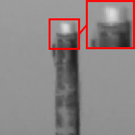
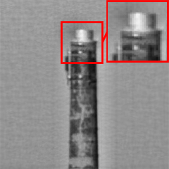
(a) Input	(b) Lucky Region	(c) Anan. et al. [3]
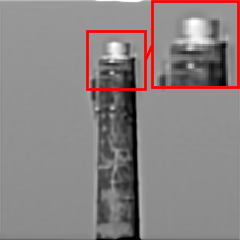
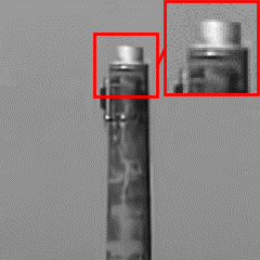
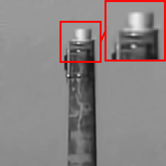
(d) Lou et al. [4]	(e) Zhu et al. [5]	(f) Ours

Figure 14: Chimney: A real static scene. The proposed method produces the sharpest recovery with minimal artifacts. Zoom-in for better visualization.

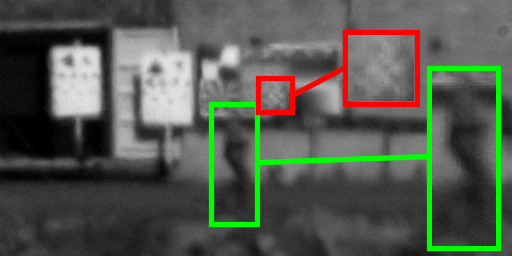
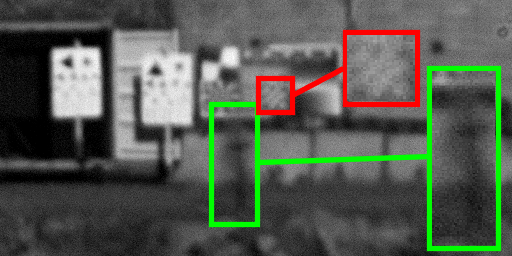
(a) Raw Input	(b) Lou et al. [4]
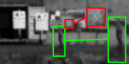
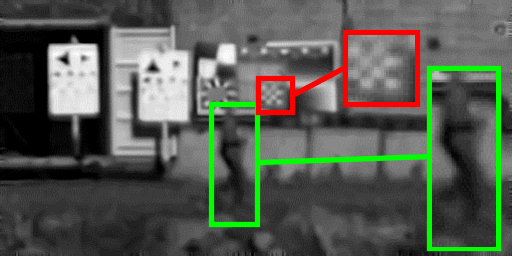
(c) Zhu et al. [5]	(d) Ours

Figure 15: Man: A real dynamic scene. The proposed method preserves the moving object while stabilizing the background turbulence. Zoom-in for better visualization.

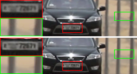
Figure 16: Car: A real dynamic scene. [Top] Raw input; Notice the blur and vibration of the background fences. [Bottom] Recovered by our proposed method. Zoom-in for better visualization.

V Conclusion

We studied the image restoration pipeline of an atmospheric turbulence problem by grounding the design parameters on the physics of the turbulence. We showed that the non-local weight parameter $\beta$ should scale with the turbulence strength $D/r_{0}$. We proved that the ratio between the shift of the PSF $\sigma$ and the PSF bandwidth $\boldsymbol{\nu}$ is upper bounded by a constant. We demonstrated how a simple prior can outperform state-of-the-art blind deconvolution algorithms in the turbulence pipeline.

Appendix A Proofs

In this section, we clarify some theoretical details in the main paper, and prove theorem 1 and proposition 1. We only provide a sketch of the proof of theorem 2 here due to space limitations, and leave the complete proof of it to the supplementary notes.

For convenience, we denote in what follows the PDF and CDF of a Normal distribution with zero mean and $\sigma^{2}$ variance as $p_{\Theta_{\sigma}}$ and $P_{\Theta_{\sigma}}$ respectively.

Recall in definition 1 we restrict the short-PSFs considered to be those defined with smoothing kernels. We provide the definition of the latter here.

Definition 2 (Smoothing Kernels).

We say a function $K:\mathbb{R}\to\mathbb{R}$ is a smoothing kernel if

1. $0\leq K(x)\leq M$ everywhere on $\mathbb{R}$;

2. $K$ is an even function;

3. $\int_{\mathbb{R}}K(x)dx<\infty$.

Remark. Our definition is inspired from, but more general than smoothing kernels studied in the theory of kernel density estimation from the probability and statistics literature, as this allows us to model more generic short-PSFs. For an introduction to the theory of kernel density estimation, see, for example, [28].

Proof of Theorem 1.

From Bernstein’s inequality stated in lemma 19 below, we have:

$$\mathbb{P}\left(\left|\widetilde{h}_{\nu}(x)-(h_{\nu}\circledast p_{\Theta})(x)\right|>\epsilon\right)$$ (16)

$$\quad\leq\,2\exp\left\{-\frac{\epsilon^{2}T}{2V_{\nu}(x,\sigma)+2\nu^{-1}M\epsilon/3}\right\}.$$

Now apply $\sup_{x\in\mathbb{R}}$ to both sides of the inequality, the left hand side is in the form we desire, and for the right hand side, based on the relationship between continuous increasing functions and the supremum operation, we have the desired expression:

$$\sup_{x\in\mathbb{R}}2\exp\left\{-\frac{T\epsilon^{2}}{2V_{\nu}(x,\sigma)+2M\nu^{-1}\epsilon/3}\right\}$$ (17)

$$\quad=\,2\exp\left\{-\frac{T\epsilon^{2}}{2\sup_{x\in\mathbb{R}}V_{\nu}(x,\sigma)+2M\nu^{-1}\epsilon/3}\right\}.$$

∎

Lemma 1.

(Bernstein’s Inequality [29])

Let $\{X_{j}\}_{j=1}^{n}$ be a collection of independent random variables. Assume $\mathbb{P}(|X_{j}|\leq M)=1$ for every $j$, and let $\mathrm{Var}[X_{j}]$ be finite for every $j$. Then for any $\epsilon>0$,

$$\mathbb{P}\left(\left|\frac{1}{n}\sum_{j=1}^{n}(X_{j}-\mathbb{E}[X_{j}])\right|>\epsilon\right)$$ (18)

$$\leq 2\exp\left\{-\frac{n\epsilon^{2}}{2\frac{1}{n}\sum_{j=1}^{n}\mathrm{Var}[X_{j}]+\frac{2}{3}M\epsilon}\right\}.$$

If the random variables are further assumed to be identically distributed, and denoting $\mathbb{E}[X_{j}]=\mu$ and $\mathrm{Var}[X_{j}]=\sigma^{2}$, then the above inequality simplifies to the following:

$$\mathbb{P}\left(\left|\frac{1}{n}\sum_{j=1}^{n}X_{j}-\mu\right|>\epsilon\right)\leq 2\exp\left\{-\frac{n\epsilon^{2}}{2\sigma^{2}+\frac{2}{3}M\epsilon}\right\}.$$ (19)

Proof of Proposition 1.

Recall by definition that $h_{\nu}(x)=\frac{1}{\nu}K(\frac{x}{\nu})$, so $h_{\nu}(x)=\frac{1}{2\nu}$ when $x\in[-\nu,\nu]$, and vanishes everywhere else. We examine $V_{\nu}(x=0,\sigma)$:

$$V_{\nu}(0,\sigma)= \int_{\mathbb{R}}h_{\nu}^{2}(0-\theta)p_{\Theta_{\sigma}}(\theta)d\theta-\left(\int_{\mathbb{R}}h_{\nu}(0-\theta)p_{\Theta_{\sigma}}(\theta)d\theta\right)^{2}$$

$$= \int_{-\nu}^{\nu}\frac{1}{4\nu^{2}}p_{\Theta_{\sigma}}(\theta)d\theta-\left(\int_{-\nu}^{\nu}\frac{1}{2\nu}p_{\Theta_{\sigma}}(\theta)d\theta\right)^{2}$$

$$= \frac{1}{4\nu^{2}}[P_{\Theta_{\sigma}}(\nu)-P_{\Theta_{\sigma}}(-\nu)]-$$

$$\quad\frac{1}{4\nu^{2}}[P_{\Theta_{\sigma}}(\nu)-P_{\Theta_{\sigma}}(-\nu)]^{2}$$

We use the common notation of $\Phi$ and $\phi$ as the cdf and pdf of the standard normal distribution respectively. Then the above expression can be rewritten as

$$V_{\nu}(0,\sigma)= \frac{1}{4\nu^{2}}\left[\Phi\left(\frac{\nu}{\sigma}\right)-\Phi\left(\frac{-\nu}{\sigma}\right)\right]-$$

$$\quad\frac{1}{4\nu^{2}}\left[\Phi\left(\frac{\nu}{\sigma}\right)-\Phi\left(\frac{-\nu}{\sigma}\right)\right]^{2}$$

$$= \frac{1}{4\nu^{2}}\left[2\Phi\left(\frac{\nu}{\sigma}\right)-1\right]-\frac{1}{4\nu^{2}}\left[2\Phi\left(\frac{\nu}{\sigma}\right)-1\right]^{2}.$$

We wish to find the interval of $\sigma$ inside $[0,\infty)$ on which $V_{\nu}$ is increasing. We note a preliminary fact that $V_{\nu}(x=0,\sigma=0)=0$, and nonnegative for $\sigma\in(0,\infty)$.

Take derivative of the above expression with respect to $\sigma$, and denoting $g_{\nu}(\sigma)=2\Phi\left(\frac{\nu}{\sigma}\right)-1$, we obtain:

$$\frac{\partial V_{\nu}}{\partial\sigma}(0,\sigma)=\frac{1}{4\nu^{2}}\frac{\partial g_{\nu}}{\partial\sigma}(\sigma)\left[1-2g_{\nu}(\sigma)\right]$$ (20)

More explicitly, using chain rule, we have

$$\frac{\partial g_{\nu}}{\partial\sigma}(\sigma)=-\frac{2\nu}{\sigma^{2}}\phi\left(\frac{\nu}{\sigma}\right)$$ (21)

Note that this expression is negative for every $\sigma\in(0,\infty)$. So to find the interval on which $V_{\nu}$ is increasing, we require the following to be true

$$1-2\left(2\Phi\left(\frac{\nu}{\sigma}\right)-1\right)=1-2g_{\nu}(\sigma)\leq 0$$ (22)

$$\iff\frac{1}{2}\leq 2\Phi\left(\frac{\nu}{\sigma}\right)-1$$

$$\iff\Phi^{-1}\left(\frac{3}{4}\right)\leq\frac{\nu}{\sigma}.$$

Since $\Phi^{-1}\left(\frac{3}{4}\right)\approx 0.67$, it holds that $\sigma\leq 1.48\nu$. Knowing that $V_{\nu}(0,\sigma)$ is continuous at $0$ (simple application of dominated convergence), it follows that on the interval $[0,1.48\nu]$, $V_{\nu}(0,\sigma)$ is increasing. ∎

Remark. The reason we only consider $V_{\nu}(0,\sigma)$ instead of $\sup_{x\in\mathbb{R}}V_{\nu}(x,\sigma)$ for the boxcar kernel case is that, from experiments we observed that for $\nu$ and $\sigma$ that is not very small, the maximizer of $V_{\nu}(x,\sigma)$ with respect to $x$ is very close to $x=0$, and for $\nu$ that is not small, $\sup_{x\in\mathbb{R}}V_{\nu}(x,\sigma)$ does not attain a global maximum at very small $\sigma$’s.

Sketch of proof of theorem 2.

There are essentially two things that we need to show:

1. The function $\sup_{x\in\mathbb{R}}V_{\nu}(x,\sigma)$ is continuous as a function of $\sigma$ on $[0,\infty)$;

2. $\sup_{x\in\mathbb{R}}V_{\nu}(x,\sigma)$ tends to $0$ when $\sigma\to\infty$

If the above two conditions hold, then with a standard argument using compact sets to exhaust $[0,\infty)$ and studying the behavior of $\sup_{x\in\mathbb{R}}V_{\nu}(x,\sigma)$ on these compact sets, the desired result follows.

Looking at the expression of $\sup_{x\in\mathbb{R}}V_{\nu}(x,\sigma)$:

$$\sup_{x\in\mathbb{R}}V_{\nu}(x,\sigma)= \sup_{x\in\mathbb{R}}\biggl{\{}\int_{\mathbb{R}}h_{\nu}^{2}(x-\theta)p_{\Theta_{\sigma}}(\theta)d\theta-$$ (23)

$$\left(\int_{\mathbb{R}}h_{\nu}(x-\theta)p_{\Theta_{\sigma}}(\theta)d\theta\right)^{2}\biggr{\}}$$

We note that, to study $\lim_{\sigma\to\sigma_{0}}\sup_{x\in\mathbb{R}}V_{\nu}(x,\sigma)$ for $\sigma_{0}\in[0,\infty]$, the basic argument of relying on the weak convergence of probability measures using the dominated convergence theorem does not really work here due to the presence of the $\sup_{x\in\mathbb{R}}$ term.

To resolve the above issue, we rely on the following classical analysis result:

Lemma 2.

Suppose we have a sequence of functions $\{g_{n}:\mathbb{R}\to\mathbb{R}\}_{n=1}^{\infty}$ that converges uniformly to a function $g:\mathbb{R}\to\mathbb{R}$, and $\sup_{x\in\mathbb{R}}g(x)<\infty$. Then the following is true:

$$\lim_{n\to\infty}\sup_{x\in\mathbb{R}}g_{n}(x)=\sup_{x\in\mathbb{R}}g(x)$$ (24)

It follows from the above lemma that, $\sup_{x\in\mathbb{R}}V_{\nu}(x,\sigma)$ is continuous at $\sigma_{0}\in[0,\infty)$ if for any sequence $\{\sigma_{n}\}_{n=1}^{\infty}$ satisfying $\sigma_{n}\to\sigma_{0}$, $V_{\nu}(x,\sigma_{n})$ tends uniformly to $V_{\nu}(x,\sigma_{0})$; similar arguments can be applied to showing $\lim_{\sigma\to\infty}\sup_{x\in\mathbb{R}}V_{\nu}(x,\sigma)=0$. However, showing uniform convergence does require more global assumptions on the function $h_{\nu}$ in addition to those stated in definition 2, namely Lipschitz continuity or continuity with compact support. We leave elaborations on these technical details to the supplementary notes. ∎

References

- [1] M. Roggemann, B. Welsh, and B. Hunt, Imaging Through Turbulence, ser. Laser & Optical Science & Technology. Taylor & Francis, 1996. [Online]. Available: https://books.google.com/books?id=nuIC-Mk0R4UC
- [2] A. Kolmogorov, “The Local Structure of Turbulence in Incompressible Viscous Fluid for Very Large Reynolds’ Numbers,” Akademiia Nauk SSSR Doklady, vol. 30, pp. 301–305, 1941.
- [3] N. Anantrasirichai, A. Achim, N. G. Kingsbury, and D. R. Bull, “Atmospheric turbulence mitigation using complex wavelet-based fusion,” IEEE Transactions on Image Processing, vol. 22, no. 6, pp. 2398–2408, June 2013.
- [4] Y. Lou, S. Ha Kang, S. Soatto, and A. Bertozzi, “Video stabilization of atmospheric turbulence distortion,” Inverse Problems and Imaging, vol. 7, no. 3, pp. 839–861, Aug. 2013.
- [5] X. Zhu and P. Milanfar, “Removing atmospheric turbulence via space-invariant deconvolution,” IEEE Transactions on Pattern Analysis and Machine Intelligence, vol. 35, no. 1, pp. 157–170, Jan. 2013.
- [6] R. Tyson, Principles of Adaptive Optics, ser. Series in Optics and Optoelectronics. CRC Press, 2010. [Online]. Available: https://books.google.com/books?id=x1PUYBvHHqcC
- [7] J. Gilles and S. Osher, “Wavelet burst accumulation for turbulence mitigation,” Journal of Electronic Imaging, vol. 25, p. 033003, May 2016.
- [8] R. C. Hardie, M. A. Rucci, A. J. Dapore, and B. K. Karch, “Block matching and wiener filtering approach to optical turbulence mitigation and its application to simulated and real imagery with quantitative error analysis,” Optical Engineering, vol. 56, no. 7, p. 071503, 2017. [Online]. Available: https://doi.org/10.1117/1.OE.56.7.071503
- [9] C. P. Lau, Y. H. Lai, and L. M. Lui, “Restoration of atmospheric turbulence-distorted images via RPCA and quasiconformal maps,” Inverse Problems, Mar. 2019.
- [10] R. P. J. Nieuwenhuizen, A. W. M. van Eekeren, J. Dijk, and K. Schutte, “Dynamic turbulence mitigation with large moving objects,” Proceedings of SPIE, vol. 10433, p. 104330S, Oct. 2017. [Online]. Available: https://doi.org/10.1117/12.2277840
- [11] C. S. Huebner, “Turbulence mitigation of short exposure image data using motion detection and background segmentation,” Proceedings of SPIE, vol. 8355, p. 83550I, May 2012. [Online]. Available: https://doi.org/10.1117/12.918255
- [12] O. Oreifej, X. Li, and M. Shah, “Simultaneous video stabilization and moving object detection in turbulence,” IEEE Transactions on Pattern Analysis and Machine Intelligence, vol. 35, no. 2, pp. 450–462, Feb. 2013.
- [13] K. K. Halder, M. Tahtali, and S. G. Anavatti, “Geometric correction of atmospheric turbulence-degraded video containing moving objects,” Optics Express, vol. 23, no. 4, pp. 5091–5101, Feb 2015. [Online]. Available: http://www.opticsexpress.org/abstract.cfm?URI=oe-23-4-5091
- [14] N. Anantrasirichai, A. Achim, and D. R. Bull, “Atmospheric turbulence mitigation for sequences with moving objects using recursive image fusion,” Aug. 2018, available online at: https://arxiv.org/abs/1808.03550.
- [15] Z. Li, Z. Murez, D. Kriegman, R. Ramamoorthi, and M. Chandraker, “Learning to see through turbulent water,” in 2018 IEEE Winter Conference on Applications of Computer Vision (WACV), Mar. 2018, pp. 512–520.
- [16] Z. Wen, A. Lambert, D. Fraser, and H. Li, “Bispectral analysis and recovery of images distorted by a moving water surface,” Applied Optics, vol. 49, no. 33, pp. 6376–6384, Nov. 2010.
- [17] D. R. Droege, R. C. Hardie, B. S. Allen, A. J. Dapore, and J. C. Blevins, “A real-time atmospheric turbulence mitigation and super-resolution solution for infrared imaging systems,” Proceedings of SPIE, vol. 8355, pp. 83 550R–1 – 83 550R–17, 2012.
- [18] D. Kamenetsky, S. Y. Yiu, and M. Hole, “Image enhancement for face recognition in adverse environments,” 2018 Digital Image Computing: Techniques and Applications (DICTA), pp. 1–6, 2018.
- [19] S. Zhao, B. Wang, L. Gong, Y. Sheng, W. Cheng, X. Dong, and B. Zheng, “Improving the atmosphere turbulence tolerance in holographic ghost imaging system by channel coding,” Journal of Lightwave Technology, vol. 31, no. 17, pp. 2823–2828, Sep. 2013.
- [20] C. Liu, “Beyond pixels: Exploring new representations and applications for motion analysis.” Ph.D. dissertation, Massachusetts Institute of Technology, Jan. 2009.
- [21] M. Aubailly, M. A. Vorontsov, G. W. Carhart, and M. T. Valley, “Automated video enhancement from a stream of atmospherically-distorted images: the lucky-region fusion approach,” Proceedings of SPIE, vol. 7463, p. 74630C, Aug. 2009. [Online]. Available: https://doi.org/10.1117/12.828332
- [22] D. L. Fried, “Statistics of a geometric representation of wavefront distortion,” Journal of the Optical Society of America, vol. 55, no. 11, pp. 1427–1435, Nov. 1965. [Online]. Available: http://www.osapublishing.org/abstract.cfm?URI=josa-55-11-1427
- [23] S. H. Chan, X. Wang, and O. A. Elgendy, “Plug-and-play ADMM for image restoration: Fixed-point convergence and applications,” IEEE Transactions on Computational Imaging, vol. 3, no. 1, pp. 84–98, 2017.
- [24] Q. Shan, J. Jia, and A. Agarwala, “High-quality motion deblurring from a single image,” ACM Transactions on Graphics (SIGGRAPH), vol. 27, no. 3, Aug. 2008.
- [25] X. Xu, J. Pan, Y. Zhang, and M. Yang, “Motion blur kernel estimation via deep learning,” IEEE Transactions on Image Processing, vol. 27, no. 1, pp. 194–205, Jan. 2018.
- [26] A. Chakrabarti, “A neural approach to blind motion deblurring,” in European Conference on Computer Vision, B. Leibe, J. Matas, N. Sebe, and M. Welling, Eds. Cham: Springer International Publishing, 2016, pp. 221–235.
- [27] M. Hirsch, S. Sra, B. Schölkopf, and S. Harmeling, “Efficient filter flow for space-variant multiframe blind deconvolution,” in The IEEE Conference on Computer Vision and Pattern Recognition (CVPR), June 2010, pp. 607–614.
- [28] L. Wasserman, All of Statistics: A Concise Course in Statistical Inference. New York, NY: Springer Science+Business Media, Inc., 2004.
- [29] S. N. Bernstein, The Theory of Probabilities. Moscow: Gastehizdat Publishing House, 1946.