Optimizing Sequential Medical Treatments with Auto-Encoding Heuristic Search in POMDPs

Abstract

Health-related data is noisy and stochastic in implying the true physiological states of patients, limiting information contained in single-moment observations for sequential clinical decision making. We model patient-clinician interactions as partially observable Markov decision processes (POMDPs) and optimize sequential treatment based on belief states inferred from history sequence. To facilitate inference, we build a variational generative model and boost state representation with a recurrent neural network (RNN), incorporating an auxiliary loss from sequence auto-encoding. Meanwhile, we optimize a continuous policy of drug levels with an actor-critic method where policy gradients are obtained from a stablized off-policy estimate of advantage function, with the value of belief state backed up by parallel best-first suffix trees. We exploit our methodology in optimizing dosages of vasopressor and intravenous fluid for sepsis patients using a retrospective intensive care dataset and evaluate the learned policy with off-policy policy evaluation (OPPE). The results demonstrate that modelling as POMDPs yields better performance than MDPs, and that incorporating heuristic search improves sample efficiency.

1 Introduction

Many recent examples Gulshan et al. (2016); Esteva et al. (2017); Litjens et al. (2017) have demonstrated above-human performance of machine learning in classification-based diagnostics. However, the investigation in sequential treatment has not been as mature due in large part to the lack of available patient-clinician interaction trajectories. Automatic treatment optimization based on reinforcement learning (RL) has been explored in simulated patients Ernst et al. (2006); Bothe et al. (2013); Lowery and Faisal (2013). Public-available electronic healthcare records allow medical sequential decisions to be learned from real-world experiences Shortreed et al. (2011); Asoh et al. (2013); Lizotte and Laber (2016); Prasad et al. (2017), even achieving human-comparable performance Komorowski et al. (2018).

Patient-clinician interactions in these works are all modelled as Markov decision processes (MDPs). Nevertheless, what we actually can observe are patient variables, without access to the relations between them and genuine physiological states, not to mention the noisiness and inherent limitations of the apparatus undertaking the measurements, the omission of relevant factors, the incongruity of the frequencies and of the time-lags among the considered measurements, etc. In contrast, POMDP Sondik (1978) agent circumvents assumptions on any of the aforementioned phenomena by optimizing actions based on information inferred over history observations, actions and feedback rewards. In addition, under POMDP there’s no necessity to interpolate for missing data, which could just be viewed as part of the intrinsic environmental obscurity, saving incidental inaccuracies incurred by data imputation. Moreover, as we may not want to involve too much manual effort in designing rewards signals, real-world problems are more often sparse-reward tasks, introducing learning lags that harm generalization efficiency.

Algorithms in POMDPs suffer notoriously from computational complexity because the history space grows exponentially in planning horizon. Alternatively, a more memory-efficient approach Cassandra et al. (1994) is to base action selection on a probability distribution in the latent state space given history trajectory, or the belief state $b_{t}=P(s|\big{\{}a_{0},o_{1},\dots,a_{t-1},o_{t}\big{\}},b_{0})$ , where $s,~{}a,~{}o,~{}b_{0}$ denote the latent environment state, action, observation and an initial belief, respectively. The belief state is a sufficient statistic for history, and can be inferred incrementally. Hauskrecht and Fraser (2000); Tsoukalas et al. (2015); Nemati et al. (2016) build POMDP frameworks in medical context but nevertheless assume discrete observation and/or action spaces and impute trivial structures on environment dynamics.

Neural networks are used in RL to either learn nontrivial dynamics or bypass environment modelling by approximating the action-value function $Q$ in $Q$-learning, or the state-value function $V$ and a parametric policy in actor-critic Mnih et al. (2015); Barth-Maron et al. (2018); Horgan et al. (2018). In addition to these function approximators, RNNs have been used in POMDPs to encode history Hausknecht and Stone (2015); Zhu et al. (2017) or belief transition Igl et al. (2018), as in POMDPs policies need to account for historical information. However, most deep RL approaches thrive on the idealistic context of large amounts of cheap training data, unlike many real-world settings such as medical ones.

We aim to develop data-efficient POMDP agents for medical applications, and stable in the potential confrontation of significantly off-policy learning from clinicians’ decisions. Specifically, each encountered belief state is evaluated through parallel suffix trees. We propose a look-ahead policy $\hat{\pi}$ to guide tree expansions that integrates the environment information embodied by a generative model into the RL agent. The belief values in the tree are subsequently back-propagated in a bottom-up fashion by Bellman update, with the values of the leaf nodes provided by current value function approximation. The value of a belief state estimated from the above simulations is closer to the true optimal value than from the value function approximation, and thus is used as the approximation target for the latter. The target policy $\pi$ is then updated through actor-critic, with policy gradient calculated from an advantage estimate. And we draw on recent literature Munos et al. (2016); Wang et al. (2016); Schulman et al. (2016) in gradient computation to not only assuage the bias-variance dilemma introduced by the discrepancy, i.e., off-policyness, between $\pi$ and clinicians’ behavior policy $\mu$ that actually generated the trajectories, but also enable more efficient gradient propagation despite reward sparsity.

We implement auto-encoding sequential Monte Carlo Le et al. (2018); Igl et al. (2018) to learn a generative model, with history dependencies regulated by an unrolled RNN. The inferred posterior distribution over the latent environment state space is represented by a particle filter. To pass an argument for policy learning, we aggregate information in the particle filter into a belief state. The evidence lower bound (ELBO) to the POMDP modelling and the RL loss within a mini batch are integrated to update all parameters simultaneously.

We evaluate our approach, auto-encoding heuristic search (AEHS), on a retrospective hospital database Medical Information Mart for Intensive Care Clinical Database (MIMIC-III) for optimizing sepsis treatment, learned from different numbers of observed patient variables that indicate levels of data obscurity. We demonstrate that including heuristics reduces the number of patient variables required to outperform clinicians’ behavior policy, and that the POMDP is a more appropriate framework than MDP for patient trajectories.

2 Related Work

Earlier POMDP algorithms are built upon known model dynamics and in discrete spaces, focusing on efficient $\alpha$-vectors representations of belief value functions Cassandra et al. (1994); Littman et al. (1995); Cassandra et al. (1997); Hauskrecht (2000); Pineau et al. (2003); Spaan and Vlassis (2004); Smith and Simmons (2004a); Ross and Chaib-Draa (2007); Kurniawati et al. (2008).

For unknown environments, Bayesian approaches Ross et al. (2007); Doshi-Velez et al. (2015), active learning Doshi-Velez et al. (2012) and spectral methods Azizzadenesheli et al. (2016) are explored for POMDPs to learn a model. Doshi-velez (2009) learns a set of infinite hidden Markov models and iteratively updates the weight of each. These approaches are however constrained to explicit structures of model dynamics, and are thus not scalable to larger spaces.

To handle large or continuous spaces, Coquelin et al. (2009) represents belief state with a weighted particle filter, and Silver and Veness (2010) with an unweighted one, both however built upon existing environment dynamics, and omission to state uncertainty after each transition by planning over a weighted average of the particles. Moreover, represented merely as a vector random variable, their environment state might be hard to infer from history.

Owing to its capacity for processing sequences, RNNs are utilized in POMDPs to encode histories to action advantages Bakker (2001), action probabilities Wierstra et al. (2007), features in addition to latest observation and action Zhang et al. (2015), or an intermediate layer in deep $Q$-networks (DQNs) Hausknecht and Stone (2015); Zhu et al. (2017).

However, back-propagation through time (BPTT) over long distances is notoriously susceptible to gradient vanishing/exploding. Recent works have also investigated appropriate initial states Kapturowski et al. (2019) or shortening BPTT length Trinh et al. (2018). Alternatively, RNNs can be involved merely in an auxiliary task. Unsupervised auxiliary losses have been demonstrated capable of finding meaningful signals from unknown environments conducive to learning the main task Jaderberg et al. (2016). For example, the DVRL in Igl et al. (2018) exploits auxiliary loss from sequence modelling to facilitate posterior inference, with state representation augmented by an RNN.

We propose a novel POMDP solution. Similarly to the DVRL, we conduct belief inference under a sequential variational model, and optimize actions in the inferred belief state. In the meantime, we formalize an efficient search mechanism in computing gradients for value function to improve data efficiency, and a stablized estimation of advantage function in computing those for policy to account for both policy discrepancy and reward-sparsity.

3 Preliminary

This section introduces recently-proposed elements that we employ to build a generative model for a sequential system and for RL online planning. For more detailed information, we refer readers to the original papers.

3.1 Sequential Monte Carlo & Auto-encoding

Sequential Monte Carlo (SMC) Doucet and Johansen (2009) is an efficient tool for performing posterior inference in structured probabilistic models of series data.

Consider a sequence of latent variables $s_{0:t}$, a sequence of observed variables $o_{1:t}$, a generative model that consists of a transition density $p_{\theta}(s_{t}|s_{0:t-1})$, an observation density $p_{\theta}(o_{t}|s_{0:t})$, an initial density $p_{\theta}(s_{0})$, characterized by parameters $\theta$, and an encoder parameterized by $\phi$, $q_{\phi}(s_{t}|o_{1:t},s_{0:t-1})$. The joint likelihood is

$$p_{\theta}(s_{0:t},o_{1:t})=p_{\theta}(s_{0})\prod_{\tau=1}^{t}p_{\theta}(s_{\tau}|s_{0:\tau-1})p_{\theta}(o_{\tau}|s_{0:\tau})$$ (1)

The target posterior distribution we want to perform inference over is

$$p_{\theta,\phi}(s_{0:t}|o_{1:t})=p_{\theta}(s_{0})\prod_{\tau=1}^{t}q_{\phi}(s_{\tau}|o_{1:\tau},s_{0:\tau-1})$$ (2)

Maintaining a set of $K$ weighted particles $\left\langle s_{0:t}^{k},w_{t}^{k}\right\rangle$ at each time step, an unbiased estimator of the marginal likelihood $p_{\theta,\phi}(o_{1:t})$ can be calculated from the weights $w^{1:K}_{1:t}$

$$\hat{p}_{\theta,\phi}^{\mathrm{SMC}}(o_{1:t};x_{0:t-1}^{1:K},s_{0:t}^{1:K})=\prod_{\tau=1}^{t}\big{(}\frac{1}{K}\sum_{k=1}^{K}w_{\tau}^{k}\big{)}$$ (3)

when the particle filter is updated by the following procedure, i.e. mutation-selection:

1) resample index $x^{k}_{t-1}$ from predecessor set $x^{k}_{t-1}\sim w^{x^{k}_{t-1}}_{t-1}/\sum_{i=1}^{K}w^{i}_{t-1}$ (selection)

$$\left.\begin{aligned} 2)&\mathrm{~{}sample~{}new~{}state~{}}s^{k}_{t}\sim q_{\phi}(\cdot|o_{1:t},s_{0:t-1}^{x^{k}_{t-1}})\\ 3)&\mathrm{~{}update~{}particle~{}}s^{k}_{0:t}\leftarrow(s_{0:t-1}^{x^{k}_{t-1}},s^{k}_{t})\\ 4)&\mathrm{~{}calculate~{}}w_{t}^{k}=\frac{p_{\theta}(s_{t}^{k}|s^{x^{k}_{t-1}}_{0:t-1})p_{\theta}(o_{t}|s^{k}_{0:t})}{q_{\phi}(s^{k}_{t}|o_{1:t},s^{x^{k}_{t-1}}_{0:t-1})}\end{aligned}\right\}\mathrm{mutation}~{}~{}~{}~{}~{}~{}~{}~{}~{}~{}~{}~{}~{}~{}~{}~{}~{}~{}~{}~{}~{}~{}~{}~{}~{}~{}~{}~{}~{}~{}~{}~{}~{}~{}~{}~{}~{}~{}~{}~{}~{}$$

until $K$ particles are updated. The posterior can be now approximated as $\sum_{k=1}^{K}w^{k}_{t}\delta_{s_{0:t}^{k}}(s_{0:t})/\sum_{k=1}^{K}w^{k}_{t}$, where $\delta_{s_{0:t}^{k}}$ is a Dirac delta distribution concentrated at $s_{0:t}^{k}$.

Given observation $o$, a generator $p_{\theta}(s,o)$ and an inference approximate $q_{\phi}(s|o)$, the Monte Carlo objective Mnih and Rezende (2016); Maddison et al. (2017) with $K$ particles is a lower bound to $\log p_{\theta}(o)$ according to Jensen’s inequality

$$\log p_{\theta}(o) \geq\mathbb{E}_{s\sim q_{\phi}}\Big{[}\log\frac{p_{\theta}(o|s)p_{\theta}(s)}{q_{\phi}(s|o)}\Big{]}$$

$$=\int\prod_{k=1}^{K}q_{\phi}(s^{k}|o)\log\frac{1}{K}\sum_{k=1}^{K}\frac{p_{\theta}(s^{k},o)}{q_{\phi}(s^{k}|o)}\textnormal{d}s^{1:K}$$ (4)

Auto-encoding SMC Le et al. (2018) formalizes the ELBO objective for $\log p_{\theta}(o_{1:t})$ developed based on the estimator Eq.(3) as

$$\mathrm{ELBO} =\int\int\prod_{k=1}^{K}p_{\theta}(s_{0}^{k})\prod_{\tau=1}^{t}\prod_{k=1}^{K}\frac{q_{\phi}(s_{\tau}^{k}|o_{1:\tau},s_{0:\tau-1}^{x^{k}_{\tau-1}})w_{\tau-1}^{x^{k}_{\tau-1}}}{\sum_{k=1}^{K}w_{\tau-1}^{k}}\log\hat{p}_{\theta,\phi}^{\mathrm{SMC}}(o_{1:t};x_{0:t-1}^{1:K},s_{0:t}^{1:K})\mathrm{d}x_{0:t-1}^{1:K}\mathrm{d}s_{0:t}^{1:K}$$

$$=\mathbb{E}_{x_{0:t-1}^{1:K},s_{0:t}^{1:K}\sim Q_{\mathrm{SMC}}}\Big{[}\sum_{\tau=1}^{t}\log\big{(}\frac{1}{K}\sum_{k=1}^{K}w_{\tau}^{k}\big{)}\Big{]}$$ (5)

where $Q_{\mathrm{SMC}}$ is the distribution of SMC. The goal of model learning at time $t,~{}t\geq 1$ is to maximize the lower bound to $\log p_{\theta}(o_{1:t})$, or minimize its negative

$$\mathcal{L}_{\mathrm{ELBO}}^{\theta,\phi}=-\frac{1}{t}\sum_{\tau=1}^{t}\log\big{(}\frac{1}{K}\sum_{k=1}^{K}w_{\tau}^{k}\big{)}$$ (6)

If stationary state distribution $Q_{\mathrm{SMC}}$ is assumed, $\sum_{\tau=1}^{t}$ in Eq.(3.1) can be taken outside of the expectation, Eq.(6) thus becomes an additive objective, allowing update using fractions of traces.

3.2 Policy Gradient

Under an MDP framework where environment state $s$ is fully observable, the goal of an RL agent is to maximize the expected long-term reward, or return $R_{t}=\sum_{\tau=t}\gamma^{\tau-t}r_{\tau}$, through optimizing a policy $\pi(a_{t}|s_{t})$ in each state. State value under $\pi$ is defined as $V^{\pi}(s)=\mathbb{E}_{\pi}\big{[}\sum_{\tau=t}\gamma^{\tau-t}r_{\tau}|s_{t}=s\big{]}$ and state-action value as $Q^{\pi}(s,a)=\mathbb{E}_{\pi}\big{[}\sum_{\tau=t}\gamma^{\tau-t}r_{\tau}|s_{t}=s,a_{t}=a\big{]}$. The subscript $\pi$ denotes the action at each step dictated by $a_{t}\sim\pi(\cdot|s_{t})$, and the stationary distribution over states implied accordingly.

Instead of learning $Q^{\pi}(s,a)$ which requires sufficient visits of all $a\in\mathcal{A}$ in each $s$, policy gradient methods explicitly represent $\pi$ with parameters $\omega$, and update them in the direction of $\mathbb{E}_{\pi}\big{[}\nabla_{\omega}V^{\pi}(s_{0})\big{]}=\mathbb{E}_{\pi}\big{[}\sum_{t=0}\gamma^{t}\nabla_{\omega}\log\pi(a_{t}|s_{t},\omega_{t})R_{t}\big{]}=\mathbb{E}_{\pi}\big{[}\sum_{t=0}\gamma^{t}\nabla_{\omega}\log\pi(a_{t}|s_{t},\omega_{t})Q^{\pi}(s_{t},a_{t})\big{]}$. Whereas $R_{t}$ based gradient estimator introduces lower bias but higher variance, function approximation based estimator incurs lower variance but higher bias Wang et al. (2016). The two can be combined for bias-variance trade-off by subtracting a state-dependent but action-independent baseline $v_{t}$ from the state-action value estimate $q_{t}$ s.t. $\mathbb{E}_{\pi}\big{[}q_{t}|s_{t},a_{t}\big{]}=Q^{\pi}(s_{t},a_{t})$, to assuage variance, and calculating $q_{t}$ from reward or trace of rewards, i.e., bootstrapping, to reduce bias.

Classically the baseline $v_{t}$ is chosen as a function approximator $V_{\kappa}(s_{t})$ that approximates $V^{\pi}(s_{t})$ Sutton and Barto (1998); Wang et al. (2016); Mnih et al. (2016); Espeholt et al. (2018). In this scenario, the difference is an estimate of the advantage function $A^{\pi}(s_{t},a_{t})=Q^{\pi}(s_{t},a_{t})-V^{\pi}(s_{t})$. The asynchronous advantage actor-critic (A3C) Mnih et al. (2016) proposes an on-policy estimate of the advantage function from a $k$-step forward-view temporal difference (TD) residual

$$\hat{A}^{\mathrm{A3C}}(s_{t},a_{t})=\sum_{i=0}^{k-1}\gamma^{i}r_{t+i}+\gamma^{k}V_{\kappa}(s_{t+k})-V_{\kappa}(s_{t})$$ (7)

The policy gradient at time $t$ can subsequently be calculated as $\nabla_{\omega}\log\pi(a_{t}|s_{t},\omega_{t})\hat{A}^{\mathrm{A3C}}(s_{t},a_{t})$.

4 Auto-Encoding Heuristic Search

This section introduces our method of sequential environment learning and heuristics in online planning. Pseudocode is provided in the supplementary material.

4.1 Belief Update

Generalization over belief states is more appropriate than over history trajectories as different histories may well result in more similar beliefs. Belief at each step is determined by the transition and observation functions of the environment from predecessor belief, latest action and current observation

$$b_{t}=\frac{p(o_{t}|s_{t},a_{t-1})\int p(s_{t}|s_{t-1},a_{t-1})b_{t-1}\mathrm{d}s_{t-1}}{\int p(o_{t}|s_{t},a_{t-1})\int p(s_{t}|s_{t-1},a_{t-1})b_{t-1}\mathrm{d}s_{t-1}\mathrm{d}s_{t}}$$

As with all posterior distributions, inference in non-trivial models require approximate approaches, among which SMC has shown remarkable performances Doucet and Johansen (2009); Coquelin et al. (2009); Silver and Veness (2010). Igl et al. (2018) adapted SMC to learning belief state by incarnating the mutation step in SMC as an RNN, with another latent random variable $z_{t}$ that adds stochasticity

$$h_{t}=\Upsilon_{\mathrm{RNN}}(h_{t-1},z_{t},a_{t-1},o_{t}|\theta)$$ (8)

where $(z_{t},a_{t-1},o_{t})$ is the input of the RNN at time $t$. The environment state is thereby the assembly of both latent variables $s_{t}=(h_{t},z_{t})$, associated with an importance weight $w_{t}^{k}$ that indicates how likely this particular sample is given historical trajectory.

Taking account of the RNN-boosted state representation, and the actions which are learned by the RL agent, the auto-encoding SMC becomes a generative model whose decoder, characterized by parameters $\theta$, consists of the transition function $p_{\theta}(z_{t}|h_{t-1},a_{t-1})$, observation function $p_{\theta}(o_{t}|z_{t},h_{t-1},a_{t-1})$, initial density in $h$ space $p_{\theta}(h_{0})$, and latent state transition $\Upsilon_{\mathrm{RNN}}(h_{t-1},z_{t},a_{t-1},o_{t}|\theta)$; and whose encoder characterized by parameters $\phi$ $q_{\phi}(z_{t}|h_{t-1},a_{t-1},o_{t})$ depends on history. The joint model likelihood conditional on actions $a_{0:t}$ is

$$p_{\theta}(h_{0:t},z_{1:t}, o_{1:t}|a_{0:t})=$$

$$p_{\theta}(h_{0})\cdot\prod_{\tau=1}^{t}p_{\theta}(z_{\tau}|h_{\tau-1},a_{\tau-1})p_{\theta}(o_{\tau}|z_{\tau},h_{\tau-1},a_{\tau-1})\delta_{\Upsilon_{\mathrm{RNN}}(h_{\tau-1},z_{\tau},a_{\tau-1},o_{\tau}|\theta)}(h_{\tau})$$ (9)

where $\delta_{\Upsilon_{\mathrm{RNN}}(h_{\tau-1},z_{\tau},a_{\tau-1},o_{\tau}|\theta)}$ represents RNN state transition density. The belief state $b_{t}$ is a posterior distribution of the above model in the space of $(h_{t},z_{t})$.

To update a particle $s_{t}^{k}=(h_{t}^{k},z_{t}^{k})$, we first resample a predecessor from previous set $h_{t-1}^{x_{t-1}^{k}}$ according to relative importance weights. A $z_{t}^{k}$ is then sampled from $q_{\phi}(\cdot|h_{t-1}^{x_{t-1}^{k}},a_{t-1},o_{t})$ using the reparameterization trick. Then we pass $(z_{t}^{k},a_{t-1},o_{t})$ into $\Upsilon_{\mathrm{RNN}}$ whose last state is $h_{t-1}^{x_{t-1}^{k}}$ and get the new state $h_{t}^{k}$, and compute corresponding $w_{t}^{k}$. The procedure $b_{t}=\mathrm{UPDATE}(b_{t-1},a_{t-1},o_{t})$ is encapsulated as follows:

1) resample index $x^{k}_{t-1}$ from predecessor set $x^{k}_{t-1}\sim w^{x^{k}_{t-1}}_{t-1}/\sum_{i=1}^{K}w^{i}_{t-1}$

2) sample latent variable $z^{k}_{t}\sim q_{\phi}(\cdot|h_{t-1}^{x^{k}_{t-1}},a_{t-1},o_{t})$

3) update RNN state $h^{k}_{t}\leftarrow\Upsilon_{\mathrm{RNN}}(h_{t-1}^{x^{k}_{t-1}},z_{t}^{k},a_{t-1},o_{t}|\theta)$

4) calculate $w_{t}^{k}=\frac{p_{\theta}(z_{t}^{k}|h^{x^{k}_{t-1}}_{t-1},a_{t-1})p_{\theta}(o_{t}|z^{k}_{t},h^{x^{k}_{t-1}}_{t-1},a_{t-1})}{q_{\phi}(z^{k}_{t}|h_{t-1}^{x^{k}_{t-1}},a_{t-1},o_{t})}$.

$\left\langle h^{k}_{t},z^{k}_{t},w^{k}_{t}\right\rangle^{1:K}$ is a particle assembly representation of $b_{t}$. To pass an argument to $V_{\kappa}$ or $\pi$ while maintaining uncertainty in $s_{t}$ after each transition, we need to aggregate information in the particle filter. The aggregation should be a permutation-invariant operation. Supported by the conviction from Murphy et al. (2019) that a permutation-sensitive function trained with permutation sampling retains tractability without notably compromising permutation invariability, we encode each $(h_{t}^{k},z_{t}^{k},w_{t}^{k})$ through the same mechanism, and use a single permutation of the encoded features to learn the belief state. Specifically, each particle value $(h_{t}^{k},z_{t}^{k})$ and feature of weight $\varphi(w_{t}^{k})$ are encoded into a belief feature with shared neural network parameters across particles, then the $K$ belief features are further encoded into a single belief state $b_{t}$. We will use the particle filter form $\mathcal{P}_{t}=\left\langle h^{k}_{t},z^{k}_{t},w^{k}_{t}\right\rangle^{1:K}$ and $b_{t}$ interchangeably as appropriate.

4.2 Heuristics in Online Planning

Policy gradient methods have stronger convergence guarantees than $Q$-learning variants Sutton and Barto (1998) since the target policy $\pi$ and value function $V_{\kappa}$ are updated smoothly via stochastic gradient descent with respect to their respective loss functions. However, the learning is potentially substantially off-policy as the target policy $\pi$ and behavior policy $\mu$ are probably disparate. In this circumstance, bootstrapping targets after taking into account the bias correction may account for scarce update information, detrimental to the asymptotic performance given limited patient trajectories. While we need to keep the target for $\pi$ bootstrapped based on previous discussion in subsection $3.2$, we compute the target for $V_{\kappa}$ from parallel heuristic search trees. Making additional use of the generative model, we evaluate each encountered belief state from model-reliant simulations to get an estimate closer to its true optimal value.

We learn a target policy via a policy gradient approach, actor-critic, representing the policy $\pi(a_{t}|b_{t},\omega_{t})$ (i.e. the actor) and belief value function $V_{\kappa}(b_{t})$ (i.e. the critic) as function approximators. We will omit $\omega$ in $\pi$ to avoid clutter.

We exploit a set of parallel best-first suffix trees, both rooted at the current belief $b_{t}$, to evaluate it through simulations. We will omit subscript $t$ in search trees because each one of them involves only one actual belief state from environment. The root has a depth of $0$, denoted as $b^{0}$.

In each tree, we expand $N_{s}$ leaf nodes, starting from $b^{0}$. $b^{d}$ is expanded by a look-ahead tree policy $a_{\mathcal{T}}$ that exploits the decoder of the current auto-encoding model: first sample a subspace of the action space $\mathcal{A}$, and resample $n_{z}$ ancestor indices $x^{i},~{}i=1,\dots,n_{z}$ from $\mathcal{P}^{d}$ (i.e. selection step), then for each $a\in\mathcal{A}$ and each $x^{i}$, sample a $z^{d+1}_{a,i}$ according to the transition $p_{\theta}(\cdot|h^{d,x^{i}},a)$, and for each $z^{d+1}_{a,i}$, simulate $n_{z,o}~{}o^{d+1}_{a,i,j}$’s from $p_{\theta}(\cdot|z^{d+1}_{a,i},h^{d,x^{i}},a)$, $j=1,\dots,n_{z,o}$. Consequently, $n_{z}\cdot n_{z,o}~{}o^{d+1}_{a,i,j}$’s will have been simulated for each $a$, each associated with a belief state $b^{d+1}_{a,i,j}=\mathrm{UPDATE}(b^{d},a,o^{d+1}_{a,i,j})$ (i.e. mutation step). Then select immediate action that conforms with

$$a_{\mathcal{T}}(b^{d})=\mathop{\mathrm{arg\,max}}_{a\in\mathcal{A}}~{}R(b^{d},a)+\frac{\gamma}{\eta^{d}(a)}\sum_{i=1}^{n_{z}}\sum_{j=1}^{n_{z,o}}\big{(}\frac{1}{K}\sum_{k=1}^{K}w^{d+1,k}_{a,i,j}\big{)}V_{\kappa}\big{(}b^{d+1}_{a,i,j}\big{)}$$

$$=\mathop{\mathrm{arg\,max}}_{a\in\mathcal{A}}~{}\Psi(b^{d},a)~{}~{}~{}~{}~{}~{}~{}~{}~{}~{}~{}~{}~{}~{}~{}~{}~{}~{}~{}~{}~{}~{}~{}~{}~{}~{}~{}~{}~{}~{}~{}~{}~{}~{}~{}~{}~{}~{}~{}~{}~{}~{}~{}~{}$$ (10)

where $R(b^{d},a)$ is the reward by choosing $a$ in $b^{d}$, and $\eta^{d}(a)=\sum_{i=1}^{n_{z}}\sum_{j=1}^{n_{z,o}}\big{(}\frac{1}{K}\sum_{k=1}^{K}w^{d+1,k}_{a,i,j}\big{)}$ is a normalization constant for $a$. Note that $\frac{1}{K}\sum_{k=1}^{K}w^{d+1,k}_{a,i,j}=\hat{p}_{\theta,\phi}(o^{d+1}_{a,i,j}|b^{d},a)$ is an unbiased estimate Eq.(3) of the marginal likelihood starting from parent $b^{d}$ conditioned on action $a$, assuming stationary distributions. Therefore, if all functions were perfectly represented and approximating the exhaustion over possible successor observations by $n_{z}\cdot n_{z,o}$ samples of $o^{d+1}_{a,i,j}$, this action would become the true optimal policy for POMDPs Ross and Chaib-Draa (2007)

$$\pi^{*}(b_{t})=\mathop{\mathrm{arg\,max}}_{a\in\mathcal{A}}R(b_{t},a)+\gamma\sum_{o_{t+1}}p(o_{t+1}|b_{t},a)V^{*}\big{(}\tau(b_{t},a,o_{t+1})\big{)}$$ (11)

where $V^{*}$ is the true optimal value function under $\pi^{*}$, and $\tau$ is the belief transition function commensurate with our $b^{d+1}_{a,i,j}=\mathrm{UPDATE}(b^{d},a,o^{d+1}_{a,i,j})$.

$\Psi(b^{d},a)$ can be thought of as a heuristic action value function that favors high-value weighted-average TD residuals with respect to the generative model. However, $\Psi$ only dictates immediate action to generate simulated experience rather than determine $\pi$ through maximization, which is known to suffer from stability and convergence issues Maei et al. (2009). To capture potential multi-modeness and encourage exploration, we convert the policy in Eq.(10) in density representation with softmax

$$\hat{\pi}\big{(}a_{\mathcal{T}}(b^{d})|b^{d}\big{)}=\frac{\exp\big{(}\Psi(b^{d},a_{\mathcal{T}}(b^{d}))/\beta\big{)}}{Z(b^{d})}$$ (12)

where $\beta$ is a temperature parameter, $Z(b^{d})=\int_{\mathcal{A}}\exp\big{(}\Psi(b^{d},a)/\beta\big{)}\mathrm{d}a$ is a partition function. After choosing $a_{\mathcal{T}}(b^{d})$, all sampled actions other than the selected one and their children are discarded.

Expansion of $b^{d}$ will therefore add $n_{z}\cdot n_{z,o}$ leaf nodes to the tree. We aim to encourage efficient expansions so that the tree is an any-time exploration mechanism. To this end, we propose expanding the node that contributes the largest payout to the root among all the leaf nodes $\mathcal{F}$: the node whose value is most likely to be back-propagated to that of the root

$$b^{*}=\mathop{\mathrm{arg\,max}}_{b\in\mathcal{F}}~{}\gamma^{D(b)}\prod_{\begin{subarray}{c}d=1\\ b^{0}\rightarrow b\end{subarray}}^{D(b)}\frac{1}{\eta^{d-1}(*)}\big{(}\frac{1}{K}\sum_{k=1}^{K}w^{d,k}\big{)}$$ (13)

where $D(b)$ is the depth of $b$, $*$ is a shorthand for the selected action, all weights and selected actions in question are from nodes in the path from root $b^{0}$ to $b$.

Once all the $N_{s}$ expansions have been investigated in silico, belief value estimates in the tree $v_{\mathcal{T}}$ are back-propagated in a bottom-up fashion to the root via Bellman update Sutton and Barto (1998); Ross and Chaib-Draa (2007)

$$v_{\mathcal{T}}(b^{d})=R\big{(}b^{d},*\big{)}+\frac{\gamma}{\eta^{d}(*)}\sum_{i=1}^{n_{z}}\sum_{j=1}^{n_{z,o}}\big{(}\frac{1}{K}\sum_{k=1}^{K}w^{d+1,k}_{*,i,j}\big{)}V_{\kappa}\big{(}b^{d+1}_{*,i,j}\big{)}$$ (14)

$\forall$ expanded $b^{d}$. Each node then has a value backed up as the weighted sum of one-step TD residuals from its direct children. The value estimates for the leaf nodes are provided by $V_{\kappa}$. $v_{\mathcal{T}}(b_{t})=v_{\mathcal{T}}(b^{0})$ is then the value estimated for $b_{t}$ from one search tree. We take the average across $N_{e}$ parallel trees $\sum_{n}^{N_{e}}v^{n}_{\mathcal{T}}(b_{t})/N_{e}$ as the target for $V_{\kappa}(b_{t})$, with the error loss being the mean-squared error between the two. If the model is exact, every application of the Bellman update makes the value estimation closer to the true optimal value Smith and Simmons (2004b). As a result, the value estimate for the root through value back-ups $v_{\mathcal{T}}(b_{t})$ is closer to $V^{*}(b_{t})$ than $V_{\kappa}(b_{t})$ is.

Gradients are only propagated from environmental interactions, not from within simulations. Therefore, the trees only provide target for $V_{\kappa}$. Note that the target for $V_{\kappa}$ is decorrelated from $\pi$, and is instead always updated towards $V^{*}$ with respect to current environment model. In on-policy case, to make $\pi$ reflect $V_{\kappa}$, the gradients of $\pi$ should be expressed by reward traces generated by $\pi$, such as Eq.(7). In off-policy case, in contrast, since the reward traces are generated by $\mu$, both the calculation and the back-propagation of the TD error $r_{s}+\gamma V_{\kappa}(b_{s+1})-V_{\kappa}(b_{s})$ at time $s$ for estimating the advantage function at time $t$ should be corrected by the difference in choosing $a_{s}$ in the two policies, or the per-decision importance sampling (IS) ratio $\frac{\pi(a_{s}|b_{s})}{\mu(a_{s}|b_{s})}$. To this end, analogously to the V-trace target introduced in Espeholt et al. (2018), we estimate the off-policy advantage function as

$$\hat{A}^{k}(b_{t},a_{t})=\sum_{s=t}^{t+k-1}\gamma^{s-t}\Big{(}\prod_{i=t}^{s-1}c_{i}\Big{)}\delta_{s}$$ (15)

where $\delta_{s}=\rho_{s}\big{(}r_{s}+\gamma V_{\kappa}(b_{s+1})-V_{\kappa}(b_{s})\big{)}$ is the TD error for $V_{\kappa}$ at time $s$ weighed by the truncated IS ratio $\rho_{s}=\min\big{(}\frac{\pi(a_{s}|b_{s})}{\mu(a_{s}|b_{s})},\rho^{-}\big{)}$, and $c_{i}=\lambda\min(\frac{\pi(a_{s}|b_{s})}{\mu(a_{s}|b_{s})},c^{-})$ is a further contracted IS ratio as is in Retrace Munos et al. (2016). The contractions effectively mitigate variance in the IS ratios, for details of which we refer readers to Munos et al. (2016); Espeholt et al. (2018). The IS ratio $\rho_{s}$ within the definition of $\delta_{s}$ corrects bias inflicted by off-policyness, while $\prod_{i=t}^{s-1}c_{i}$ further reduces the impact of bias at time $s$ on the advantage estimate at $t$. This is similar to the generalized advantage estimator proposed in Schulman et al. (2016), the distinction being that we correct bias by coefficient $c_{i}$ instead of a constant $\lambda$.

The superscript $k$ in Eq.(15) denotes the estimate is calculated from an up-to-$k$ step trace. However, as we frame the medical application as a sparse-reward situation (details in the supplementary material), only the transitions to terminals being linked to non-zero rewards, we back-propagate these rewards to all previous steps in each respective trajectory. To this end, we estimate the advantage function with infinite horizon

$$\hat{A}^{\infty}(b_{t},a_{t})=\sum_{s=t}^{\infty}\gamma^{s-t}\Big{(}\prod_{i=t}^{s-1}c_{i}\Big{)}\delta_{s}$$ (16)

with a slight misusage of $\infty$ to denote the whole trajectory from $t$ onward till the terminal. As such, the maximum propagation length is the length of each admission trajectory.

4.3 Learning Objective

This subsection summarizes loss functions for training parameters jointly, with derivations spread over previous subsections. Admission trajectories are concatenated together. The mini batch size is denoted as $L$.

The loss introduced by model learning is

$$\mathcal{L}_{\mathrm{ELBO}}^{\theta,\phi}=-\frac{1}{L}\sum_{\tau=t}^{t+L-1}\log\big{(}\frac{1}{K}\sum_{k=1}^{K}w_{\tau}^{k}\big{)}$$ (17)

The policy loss $\mathcal{L}^{\theta,\phi,\omega}_{\pi}$ and the value function loss $\mathcal{L}^{\theta,\phi,\kappa}_{V}$ from RL online planning are

$$\mathcal{L}^{\theta,\phi,\omega}_{\pi}=-\frac{1}{L}\sum_{\tau=t}^{t+L-1}\log\pi(a_{\tau}|b_{\tau},\omega_{\tau})\hat{A}^{\infty}(b_{\tau},a_{\tau})$$ (18)

$$\mathcal{L}^{\theta,\phi,\kappa}_{V}=\frac{1}{L}\sum_{\tau=t}^{t+L-1}\big{(}\frac{1}{N_{e}}\sum_{n}^{N_{e}}v^{n}_{\mathcal{T}}(b_{\tau})-V_{\kappa}(b_{\tau})\big{)}^{2}$$ (19)

A policy entropy bonus could be imposed to mitigate premature policy convergence like in A3C

$$\mathcal{L}^{\theta,\phi,\omega}_{H}=-\frac{1}{L}\sum_{\tau=t}^{t+L-1}\int\pi(a|b_{\tau})\log\pi(a|b_{\tau})\mathrm{d}a$$ (20)

Moreover, we estimate the behavior policy $\mu$ also from a neural network, parameterized by $\zeta$, the error loss being the negative loss probability of the actual behavior

$$\mathcal{L}^{\theta,\phi,\zeta}_{\mu}=-\frac{1}{L}\sum_{\tau=t}^{t+L-1}\log\mu(a_{\tau}|b_{\tau},\zeta_{\tau})$$ (21)

The overall loss at update time $t$ is the sum of $\mathcal{L}_{\mathrm{ELBO}}^{\theta,\phi}$, $\mathcal{L}^{\theta,\phi,\omega}_{\pi}$, $\mathcal{L}^{\theta,\phi,\kappa}_{V}$ , $\mathcal{L}^{\theta,\phi,\omega}_{H}$ and $\mathcal{L}^{\theta,\phi,\zeta}_{\mu}$ rescaled by relative weights, which are hyperparameters. Note the overall loss is only computed from one thread.

5 Experiments

We test our method on a retrospective critical care dataset, MIMIC-III, where we treat each admission as an episode. Please see the supplementary material for more information on the cohort. One of our baselines is clinicians’ behavior policy $\mu$, which we evaluate on-policy as the average empirical return of the test set. Further, to single out the advantage of involving heuristics in online planning, we compare AEHS to AE+A2C, our sequential generative model for POMDP with original synchronous A3C, or A2C, parallel workers. For AE+A2C we split all training steps (roughly) evenly into $N_{e}$ groups without breaking episodes. We also compare to when the patient-clinician interactions are modelled as MDPs by simplifying our generative model accordingly and interpolating missing data.

We use RMSProp Tieleman and Hinton (2012) as the optimizer with shared statistics across threads. The discount factor in RL is $\gamma=0.99$. We set the population size of the particle filter $K=15$ and the number of threads $N_{e}=16$ for both AEHS and AE+A2C, the times of expansions $N_{s}=20$ and mini batch size $L=10$ for AEHS, and the temporal component of batch size for AE+A2C also $L=10$, leading to a total batch size of $L\times N_{e}$. In both contestants the TD errors are back-propagated over full trajectories. Note this is different in the original A2C implementation where the bootstrapped length is upper bounded by the number of steps run ahead $L$. This way one could maximally single out the effect of heuristic search. Please see the supplementary material for implementation details.

Learning curve visualizations are averaged over $10$ training instances, each consisting of $5$ epochs of random shuffles of all patient admissions in the training set. Shaded areas represent standard deviations.

The evaluation of our learned policy $\pi(a_{t}|b_{t},\omega)$ using sequences generated by $\mu(a_{t}|b_{t})$ is an instance of off-policy policy evaluation (OPPE). We implement weighted importance sampling (WIS) Sutton and Barto (1998) as a means to correct discrepancies between the probabilities of a trajectory under the two policies considering episodic tasks. The per-trajectory IS weight is defined as $W_{n}=\prod_{t=0}^{T_{n}-1}\frac{\pi(a_{t}|b_{t},\omega)}{\mu(a_{t}|b_{t})}$, the WIS return of a dataset is estimated as $R^{\mathrm{WIS}}=\frac{\sum_{n}^{N}W_{n}R_{n}}{\sum_{n}^{N}W_{n}}$, where $R_{n}$ is the empirical return of trajectory $n$. IS weights $W_{n}$ notoriously suffer from high variance, especially when $\pi$ is significantly dissimilar to $\mu$. This is detrimental, since trajectories corresponding to extremely small weights would effectively be ignored in evaluating the whole dataset.

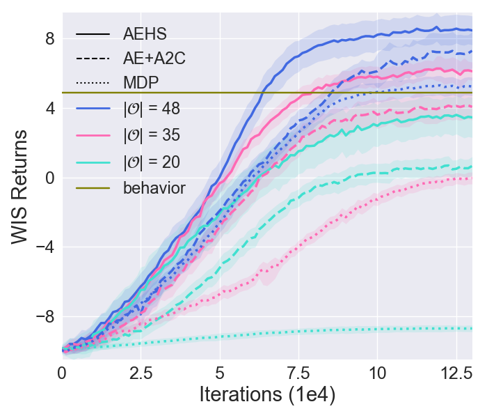
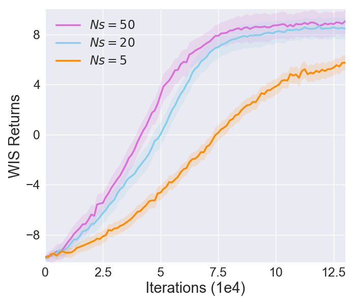
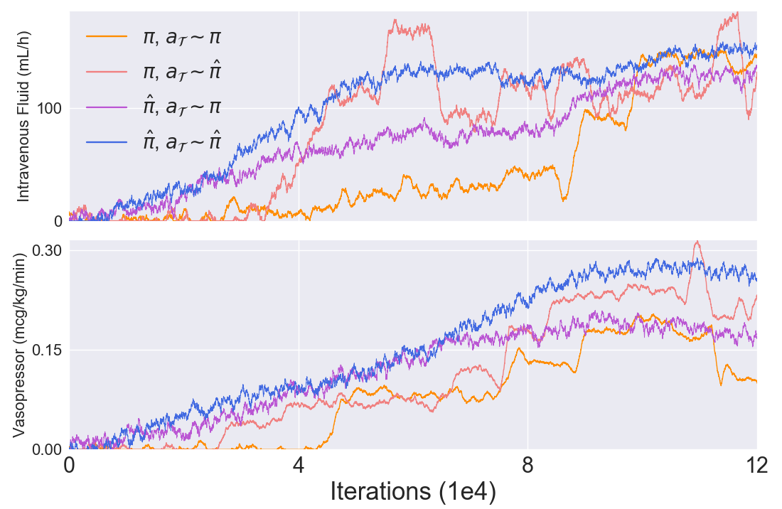
(a)	(b)	(c)

Figure 1: (a) Validations on the test set, with parameters trained from different numbers of observed patient variables as an indicator of partial observability, and from corresponding sets of patient variables while assuming full observability. Results shown are the OPPE outcome of current parameters every training iteration. (b) Influence of the number of expansions in each tree search. (c) Action updates in a single belief, when actions in search trees are dictated by $\pi$ or $\hat{\pi}$. Negative actions during test are truncated at $0$.

Some works Hanna et al. (2017); Liu et al. (2018) have been dedicated to stable OPPE approaches. As the method for policy optimization is orthogonal to that for policy evaluation, and our major investigation is in the former, we simply clip each $W_{n}$ into $[W_{-},W^{-}]$ as in Jagannatha et al. (2018). We show with bootstrapping estimates in the supplementary material confidence bounds of OPPE, that with higher truncation levels, the variance in WIS returns is lower, but the policy we end up evaluating deviates more from the actual $\pi$ and more towards $\mu$.

5.1 Overall Performance

To see our robustness to data obscurity as well as to justify the incorporation of heuristics, we choose from the set of $48$ patient variables $35$ and then from them, $20$ patient variables as observations. For all of the three sets of observations, we first model the trajectories as POMDPs and implement AEHS and AE+A2C respectively. Missing data are not interpolated for POMDPs. Then for the same three sets of observations, we use MDP model and apply to them the AEHS substituting the auto-encoding SMC with a conditional variational auto-encoder $p_{\theta}(o_{0})$, $p_{\theta}(o_{t}|z_{t},o_{t-1},a_{t-1})$ and $q_{\phi}(z_{t}|o_{t},o_{t-1},a_{t-1})$, that directly maps $o_{t-1},a_{t-1}$ into $o_{t}$. Missing data are linearly interpolated in MDPs. After each training iteration (i.e. $L$ steps), the model and RL agent is validated on the test set, with each per-trajectory IS weight clipped into $[1e-30,1e4]$.

Results in Figure 1 $(a)$ show that, modelling as MDPs is more susceptible to the number of patient variables involved and consistently yields poorer performances despite the observation dimensionality than modelling as POMDPs, vindicating that patient-clinician interactions are de facto POMDPs. Moreover, as the incompleteness of observations increases in POMDP framework, both AEHS and AE+A2C learn worse, but AEHS deteriorates slightly less than AE+A2C, and learns faster and better across all three cases. The horizontal line manifests the on-policy policy evaluation result of clinicians’ behavior policy. We note that, given limited trajectories, upon convergence AE+A2C ceases to surpass clinical baseline at $35$ patient variables, while AEHS ceases to do so at $20$ patient variables. In the supplementary material we show that with $48$ patient variables, the $95\%$ confidence lower bound on the WIS return of the test set under this specific truncation level of IS weights is $7.030$, while the average empirical return per trajectory under $\mu$ is $4.867$.

5.2 Efficiency of Heuristics

To test whether our heuristics are applied efficiently, we first investigate the influence of the number of node expansions $N_{s}$ in each suffix tree. As is shown in Figure 1 $(b)$, increasing $N_{s}$ does not dramatically boost performance. This is because the trees are best-first: Eq.(13) always selects the most influential node to expand, implying that there is no need to expand many more nodes to evaluate the root.

We then track the action values, dosages of vasopressor and of intravenous fluid, in a single belief of a single training instance. Specifically, we compare how the target policy $\pi$ is updated and how the look-ahead policy $\hat{\pi}$ would appear when selecting actions $a_{\mathcal{T}}$ by $\pi$ or $\hat{\pi}$ respectively during tree explorations, as real actions are unanimously dictated by $\mu$. The results visualized in Figure 1 $(c)$ suggest that, $\hat{\pi}$ tends to update ahead of $\pi$ like a precursor, and updates more stably on the whole. In addition, $\pi$ is able to update faster when simulations are dictated by $\hat{\pi}$ than by $\pi$. This is because $\hat{\pi}$ accounts for more information for planning than $\pi$ by probing into the values of multiple reachable belief states. Expanding the suffix trees with $\hat{\pi}$ therefore helps with the efficiency of finding a target for $V_{\kappa}$ that is closer to $V^{*}$.

6 Conclusion

We propose a novel POMDP approach to optimizing sepsis treatment from a retrospective critical care database. To encourage belief inference, we build an auto-encoding SMC and incorporate the ELBO as an auxiliary loss. Secondly, we propose a heuristic planning architecture that exploits best-first suffix trees to improve data efficiency. Thirdly, lagged learning effect induced from reward sparsity is mitigated by back-propagating over full trajectories, alongside an off-policy estimate of policy gradient is devised with bias correction and variance control. Our experimental results demonstrate that, 1) POMDP is indeed a more appropriate model for patient-clinician interactions than MDP, 2) our approach is able to surpass clinicians’ baseline by a remarkable margin with high probability in OPPE terms, and 3) our heuristics in tree policy and nodes to expand consistently improves planning performance and data efficiency.

Appendix A Implementation

We approximate transition density $p_{\theta}(z_{t}|h_{t-1},a_{t-1})$, encoder $q_{\phi}(z_{t}|h_{t-1},a_{t-1},o_{t})$ and decoder $p_{\theta}(o_{t}|z_{t},h_{t-1},a_{t-1})$ both as multivariate Gaussian distributions, each by two fully connected layers and two separate fully connected output layers for the mean and the variance respectively.

All $a$ and $o$ are encoded before passing into a network: $a$ is encoded by one fully connected layer of size $64$, and $o$ by two fully connected layers. Multiple inputs are concatenated as one vector. All covariance matrices are diagonal.

For actor-critic we use one fully connected layer followed by three output fully connected layers: one for the value function of size $1$, one for the policy mean and the other for the policy variance, both of size $2$. The behavior policy is also a fully connected layer followed by a layer for the mean and the other layer for variance.

To aggregate information in the particle filter, we first encode each weight by one fully connected layer of size $64$, and encode the corresponding particle value and the feature of weight into a belief feature by two fully connected layers. The $K$ belief features are then concatenated and encoded by a fully connected output layer in $b$ space. All network weights are shared across particles.

$z$, $h$ and $b$ all have a dimension of $128$. All other fully connected layers have a size of $128$ if not specified otherwise. RNNs are gated recurrent units (GRUs). All hidden layers are activated by rectified linear units (ReLUs). All network weights are initialized using orthogonal initializer. Batch normalization is not implemented.

We use RMSProp with shared statistics across threads as the optimizer which works well with RNNs. Momentum is not considered. The decay factor in RMSProp is $\alpha=0.99$. Gradients are truncated at the norm of $0.5$. The relative weights for $\mathcal{L}^{\theta,\phi,\kappa}_{V}$ and $\mathcal{L}^{\theta,\phi,\omega}_{H}$ are set to $0.5$ and $0.01$ as in A3C, the weight for $\mathcal{L}^{\theta,\phi}_{\mathrm{ELBO}}$ is $0.1$.

Our hyperparameters under tuning include learning rate $([1e-5,1e-3]\textnormal{~{}log uniform})$ and regularization factor $\varepsilon$ in RMSProp $([1e-5,1e-1]\textnormal{~{}log uniform})$.

Appendix B Patient Variables

Table 1: $48$ patient variables involved as observations. C: continuous/multi-valued, B: binary.

Category	Items	Type
Demographics	age (in days)	C
	gender	B
	weight (kg)	C
	readmission to intensive care	B
	elixhauser score (premorbid status)	C
Vital signs	SOFA (based on current step)	C
	SIRS	C
	Glasgow coma scale	C
	heart rate	C
	systolic blood pressure	C
	diastolic blood pressure	C
	mean blood pressure	C
	shock index	C
	respiratory rate	C
	SpO2	C
	temperature	C

Ventilation parameters	mechanical ventilation	B
	FiO2	C
Laboratory values	potassium	C
	sodium	C
	chloride	C
	magnesium	C
	calcium	C
	ionized calcium	C
	carbon dioxide	C
	glucose	C
	BUN	C
	creatinine	C
	SGOT	C
	SGPT	C
	total bilirubin	C
	albumin	C
	hemoglobin	C
	white blood cells count	C
	platelets count	C
	PTT	C
	PT	C
	INR	C
	pH	C
	PaO2	C
	PaCO2	C
	base excess	C
	bicarbonate	C
	lactate	C
Fluid balance	urine output (over $4$h)	C
	accumulated fluid balance since admission	C
Other interventions	renal replacement therapy	B
	sedation	B

Appendix C Cohort

C.1 Cohort Selection

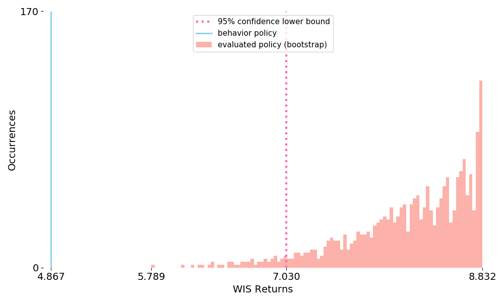
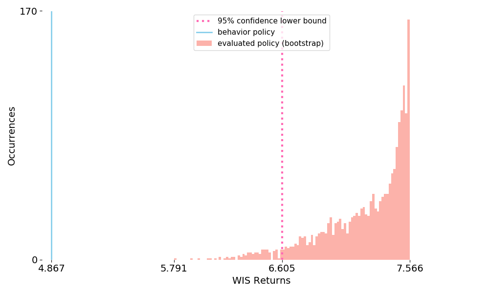
 (a)   (b)

Figure 1: Histograms on bootstrap samples of WIS return of test set. (a) when per-trajectory IS weights clipped to $[1e-30,1e4]$. (b) when per-trajectory IS weights clipped to $[1e-20,1e3]$

Our cohort is a retrospective database, Medical Information Mart for Intensive Care Clinical Database (MIMIC-III) Johnson et al. (2017) that contains de-identified health-related records of patients during their stays in a hospital ICU. We investigate the treatment optimization for sepsis, to which standard approach in current medical guidance lacks. We include data based on the same conditions as Komorowski et al. (2018), selecting adult patients in the MIMIC-III database who conform to the international consensus sepsis-3 criteria Singer et al. (2016), excluding admissions in which treatment was withdrawn or mortality was not documented. For all patients, data are extracted from up to $24$ hours preceding, and until up to $48$ hours ensuing the estimated onset of sepsis, to which the time series are aligned. Time series are temporally discretized with $4$-hour intervals, resulting in $18,914$ ICU admissions or $251,843$ steps in total. $2,000$ admissions are randomly sampled and excluded from training for evaluation.

C.2 Data Extraction

The treatments and patient variables to consider are also identical to those in Komorowski et al. (2018), recounted here for completeness, with value continuities retained. Our action space consists of the maximum dose of vasoppressors administered and the total volume of intravenous fluids injected over each $4$h time bin. The vasopressors include norepinephrine, epinephrine, vasopressin, dopamine and phenylephrine, and are converted to norepinephrine-equivalent with dose correspondence Brown et al. (2013). The intravenous fluids include boluses and background infusions of crystalloids, colloids and blood products, normalized by tonicity. Both actions are continuous. We model both $\pi$ and $\mu$ as Gaussian distributions. The output of each of the two policy networks contains two separate layers, one for the mean, one for the variance, both are two dimensional.

A table of the $48$ continuous or binary patient variables we assume to be of interest is given in Supp. Table 1. Notice that not all $48$ variables are available at each and all of the steps due to lower frequency or failure to record. We do not interpolate those missing data, treating them instead as part of partial observability of the task.

The single goal in the POMDP is survival. Transitions to the terminal discharge without deceasing in $90$ days are rewarded by $+10$, those to the terminal death, either in-hospital or $90$ days from discharge, are penalized by $-10$. No intermediate reward is set so as to encourage learning from scratch.

C.3 Data Preprocessing

For measurements among the extracted $48$ patient variables with multiple records within a $4$h time bin, records are averaged (e.g. heart rate) or summed (e.g. urine output) as appropriate. All observation and action values are normalized between $[0,1]$, action values for both drugs are then converted to $a\leftarrow a^{0.3}$ to dilate small values because smaller dosages are selected more frequently by clinicians in respective range and we want to capture nuances.

Appendix D Further OPPE

As the method for policy optimization is orthogonal to that for policy evaluation, and our major investigation is in the former, we simply clip each $W_{n}$ into $[W_{-},W^{-}]$ to reduce variance. More truncation results in lower variance, at the cost of ending up evaluating an in-between policy that is less like $\pi$ but more like $\mu$.

We exemplify two sets of truncation thresholds, $[1e-30,1e4]$ and $[1e-20,1e3]$ to show the trend. To capture variance, we estimate WIS return of the test set through bootstrapping, resampling from the set $2,000$ times, resulting in $2,000$ bootstrap estimates. Each estimate is the result of applying WIS to the resampled trajectories. The histograms of the estimates are shown in Supp. Figure 1, together with the $95\%$ confidence lower bound and the value of the behavior policy $R^{\mu}=\frac{1}{N}\sum_{n}^{N}R_{n}$. In both cases, the $95\%$ confidence lower bounds of $\pi$ value exceed the value of $\mu$ by considerable margins.

Appendix E Pseudocode

$\mathcal{P}^{*}\leftarrow\mathcal{P}_{t},~{}b^{*}\leftarrow b_{t},~{}d\leftarrow 0\mathcal{F}\leftarrow\o$

for $s=1,\dots,N_{s}$ do

       sample a subspace $\mathcal{A}$ sample ancestor indices $x^{1:n_{z}}$ from $\mathcal{P}^{*}$  for $a\in\mathcal{A}$ do

             for $i=1,\dots,n_{z}$ do

                   sample $z^{d+1}_{a,i}\sim p_{\theta}(\cdot|h^{d,x^{i}},a)$ for $j=1,\dots,n_{z,o}$ do

                         sample $o^{d+1}_{a,i,j}\sim p_{\theta}(\cdot|z^{d+1}_{a,i},h^{d,x^{i}},a)$ $\mathcal{P}^{d+1}_{a,i,j},b^{d+1}_{a,i,j}\leftarrow\mathrm{UPDATE}(\mathcal{P}^{*},a,o^{d+1}_{a,i,j})$

                   end for

                  

             end for

            $\Psi(b^{*},a)\leftarrow R(b^{*},a)+\frac{\gamma}{\eta^{d}(a)}\sum_{i=1}^{n_{z}}\sum_{j=1}^{n_{z,o}}\big{(}\frac{1}{K}\sum_{k=1}^{K}w^{d+1,k}_{a,i,j}\big{)}V_{\kappa}\big{(}b^{d+1}_{a,i,j}\big{)}$

       end for

      $\hat{\pi}(a|b^{*})\leftarrow\frac{\exp\big{(}\Psi(b^{*},a)/\beta\big{)}}{\int_{\mathcal{A}}\exp\big{(}\Psi(b^{*},a^{\prime})/\beta\big{)}\mathrm{d}a^{\prime}}$ $a_{\mathcal{T}}(b^{*})\sim\hat{\pi}(\cdot|b^{*})$ $\mathcal{F}\leftarrow\mathcal{F}\cup\big{\{}b^{d+1}_{i,j,a_{\mathcal{T}}(b^{*})},\forall i,j\big{\}}$ if $s<N_{s}$ then

             $b^{*}\leftarrow\mathop{\mathrm{arg\,max}}_{b\in\mathcal{F}}~{}\gamma^{D(b)}\prod_{\begin{subarray}{c}d=1\\ b^{0}\rightarrow b\end{subarray}}^{D(b)}\frac{1}{\eta^{d-1}(*)}\big{(}\frac{1}{K}\sum_{k=1}^{K}w^{d,k}\big{)}$ $d\leftarrow$ depth of $b^{*}$ $\mathcal{P}^{*}\leftarrow$ where $b^{*}$ is extracted

       end if

      

end for

$v_{\mathcal{T}}(b)\leftarrow V_{\kappa}(b)~{}\forall~{}b\in\mathcal{F}$ for $d=\big{(}\mathop{\mathrm{max}}_{b\in\mathcal{F}}D(b)-1\big{)},\dots,0$ do

       for $\mathrm{each~{}expanded~{}}b^{d}$ do

             $v_{\mathcal{T}}(b^{d})\leftarrow R\big{(}b^{d},*\big{)}+\frac{\gamma}{\eta^{d}(*)}\sum_{i=1}^{n_{z}}\sum_{j=1}^{n_{z,o}}\big{(}\frac{1}{K}\sum_{k=1}^{K}w^{d+1,k}_{*,i,j}\big{)}V_{\kappa}\big{(}b^{d+1}_{*,i,j}\big{)}$

       end for

      

end for

Output: $v_{\mathcal{T}}(b^{0})$  

Algorithm 1 Heuristic search tree $\mathcal{T}\big{(}\mathcal{P}_{t},~{}b_{t}\big{)}$

initialize $\theta,~{}\phi,~{}\kappa,~{}\omega,~{}\zeta$

concatenate epochs of shuffled admission trajectories

$o_{0}\leftarrow$ first observation

$\mathcal{P}_{0},~{}b_{0}\leftarrow\mathrm{INIT}(o_{0})$

$t\leftarrow 0$

repeat

       $\mathcal{L}^{\theta,\phi}_{\mathrm{ELBO}},~{}\mathcal{L}^{\theta,\phi,\kappa}_{V},~{}\mathcal{L}^{\theta,\phi,\omega}_{\pi},~{}\mathcal{L}^{\theta,\phi,\omega}_{H},\mathcal{L}^{\theta,\phi,\zeta}_{\mu}\leftarrow 0$ $t_{\mathrm{start}}\leftarrow t$ for $\tau=t,\dots,(t+L-1)$ do

             $\mathcal{L}^{\theta,\phi}_{\mathrm{ELBO}}-=\log\big{(}\frac{1}{K}\sum_{k}w^{k}_{\tau}\big{)}$ for $n=1,\dots,N_{e}\mathrm{~{}(compute~{}in~{}parallel)}$  do

                   $v^{n}_{\mathcal{T}}(b_{\tau})\leftarrow\mathcal{T}\big{(}\mathcal{P}_{\tau},~{}b_{\tau}\big{)}$

             end for

            $\mathcal{L}^{\theta,\phi,\kappa}_{V}+=\big{(}\sum_{n}^{N_{e}}v_{\mathcal{T}}^{n}(b_{\tau})/N_{e}-V_{\kappa}(b_{\tau})\big{)}^{2}$ if $\tau==\mathrm{last~{}nonterminal~{}step~{}in~{}current~{}trajectory}$ then

                   $\hat{A}^{\infty}\leftarrow 0$ for $i=\tau,\dots,t_{\mathrm{start}}$ do

                         $\delta_{i}\leftarrow\rho_{i}\big{(}r_{i}+\gamma V_{\kappa}(b_{i+1})-V_{\kappa}(b_{i})\big{)},~{}\big{(}\delta_{\tau}\leftarrow\rho_{\tau}(r_{\tau}-V_{\kappa}(b_{\tau}))\big{)}$ $\hat{A}^{\infty}\leftarrow\gamma c_{i}\hat{A}^{\infty}+\delta_{i}$ $\mathcal{L}^{\theta,\phi,\omega}_{\pi}-=\log\pi(a_{i}|b_{i})\hat{A}^{\infty}$ $\mathcal{L}^{\theta,\phi,\omega}_{H}-=\int\pi(a|b_{i})\log\pi(a|b_{i})\mathrm{d}a$ $\mathcal{L}^{\theta,\phi,\zeta}_{\mu}-=\log\mu(a_{i}|b_{i})$

                   end for

                  $t_{\mathrm{start}}\leftarrow\tau+1$ $\mathcal{P}_{\tau+1},~{}b_{\tau+1}\leftarrow\mathrm{INIT}(o_{\tau+1})$

             else

                  $\mathcal{P}_{\tau+1},~{}b_{\tau+1}\leftarrow\mathrm{UPDATE}(\mathcal{P}_{\tau},a_{\tau},o_{\tau+1})$

             end if

            

       end for

      for $s=(t+L),\dots,\mathrm{~{}last~{}nonterminal~{}step~{}in~{}current~{}trajectory}$ do

            $\_,~{}b_{s}\leftarrow\mathrm{UPDATE}(\mathcal{P}_{s-1},a_{s-1},o_{s})$

       end for

      $\hat{A}^{\infty}\leftarrow\sum_{s=t+L}^{\infty}\gamma^{s-t-L}\Big{(}\prod_{i=t+L}^{s-1}c_{i}\Big{)}\delta_{s}$ for $i=(t+L-1),\dots,t_{\mathrm{start}}$ do

             $\delta_{i}\leftarrow\rho_{i}\big{(}r_{i}+\gamma V_{\kappa}(b_{i+1})-V_{\kappa}(b_{i})\big{)}$ $\hat{A}^{\infty}\leftarrow\gamma c_{i}\hat{A}^{\infty}+\delta_{i}$ $\mathcal{L}^{\theta,\phi,\omega}_{\pi}-=\log\pi(a_{i}|b_{i})\hat{A}^{\infty}$ $\mathcal{L}^{\theta,\phi,\omega}_{H}-=\int\pi(a|b_{i})\log\pi(a|b_{i})\mathrm{d}a$ $\mathcal{L}^{\theta,\phi,\zeta}_{\mu}-=\log\mu(a_{i}|b_{i})$

       end for

      $\mathcal{L}\leftarrow\sum\mathrm{rescale}\big{(}\mathcal{L}^{\theta,\phi}_{\mathrm{ELBO}},~{}\mathcal{L}^{\theta,\phi,\kappa}_{V},~{}\mathcal{L}^{\theta,\phi,\omega}_{\pi},~{}\mathcal{L}^{\theta,\phi,\omega}_{H},\mathcal{L}^{\theta,\phi,\zeta}_{\mu}\big{)}/L$ update $\theta,\phi,\kappa,\omega,\zeta$ with $\nabla(\mathcal{L})$ $t\leftarrow t+L$

until $\mathrm{converged}$

Algorithm 2 AEHS

for $k=1,\dots,K$ do

       sample $h\sim p_{\theta}(h_{0}),~{}a\sim\mathrm{random}$ sample $z^{k}_{t}\sim q_{\phi}(\cdot|h,a,o_{0})$ $h^{k}_{t}\leftarrow\Upsilon_{\mathrm{RNN}}(h,z_{t}^{k},a,o_{t}|\theta)$ $w_{t}^{k}\leftarrow\frac{p_{\theta}(z_{t}^{k}|h,a)p_{\theta}(o_{0}|z^{k}_{t},h,a)}{q_{\phi}(z^{k}_{t}|h,a,o_{0})}$ insert $\left\langle h_{t}^{k},z_{t}^{k},w_{t}^{k}\right\rangle$ into $\mathcal{P}_{t}$

end for

aggregate information in $\mathcal{P}_{t}$ into $b_{t}$ Output: $\mathcal{P}_{t},~{}b_{t}$

Algorithm 3 Belief state initialization $\mathrm{INIT}(o_{0})$

for $k=1,\dots,K$ do

       sample $x^{k}_{t-1}\sim w^{x^{k}_{t-1}}_{t-1}/\sum_{i}w^{i}_{t-1}$ sample $z^{k}_{t}\sim q_{\phi}(\cdot|h_{t-1}^{x^{k}_{t-1}},a_{t-1},o_{t})$ $h^{k}_{t}\leftarrow\Upsilon_{\mathrm{RNN}}(h_{t-1}^{x^{k}_{t-1}},z_{t}^{k},a_{t-1},o_{t}|\theta)$ $w_{t}^{k}\leftarrow\frac{p_{\theta}(z_{t}^{k}|h^{x^{k}_{t-1}}_{t-1},a_{t-1})p_{\theta}(o_{t}|z^{k}_{t},h^{x^{k}_{t-1}}_{t-1},a_{t-1})}{q_{\phi}(z^{k}_{t}|h_{t-1}^{x^{k}_{t-1}},a_{t-1},o_{t})}$ insert $\left\langle h_{t}^{k},z_{t}^{k},w_{t}^{k}\right\rangle$ into $\mathcal{P}_{t}$

end for

aggregate information in $\mathcal{P}_{t}$ into $b_{t}$ Output: $\mathcal{P}_{t},~{}b_{t}$

Algorithm 4 Belief transition $\mathrm{UPDATE}\big{(}\mathcal{P}_{t-1},a_{t-1},o_{t}\big{)}$

References

- Asoh et al. (2013) Hideki Asoh, Masanori Shiro, Shotaro Akaho, Toshihiro Kamishima, Koiti Hasida, Eiji Aramaki, and Takahide Kohro. An application of inverse reinforcement learning to medical records of diabetes treatment. In European Conference on Machine Learning and Principles and Practice of Knowledge Discovery in Databases, Sep 2013.
- Azizzadenesheli et al. (2016) Kamyar Azizzadenesheli, Alessandro Lazaric, and Animashree Anandkumar. Reinforcement learning of pomdps using spectral methods. In 29th Annual Conference on Learning Theory, volume 49 of Proceedings of Machine Learning Research, pages 193–256, Columbia University, New York, New York, USA, 23–26 Jun 2016. PMLR.
- Bakker (2001) Bram Bakker. Reinforcement learning with long short-term memory. In Proceedings of the 14th International Conference on Neural Information Processing Systems: Natural and Synthetic, 2001.
- Barth-Maron et al. (2018) Gabriel Barth-Maron, Matthew W. Hoffman, David Budden, Will Dabney, Dan Horgan, Dhruva Tirumala, Alistair Muldal, Nicolas Heess, and Timothy P. Lillicrap. Distributed distributional deterministic policy gradients. ICLR, abs/1804.08617, 2018.
- Bothe et al. (2013) Melanie Bothe, Luke W. F. Dickens, Katrin Reichel, Arn Tellmann, Bjoern Ellger, Martin Westphal, and Aldo A. Faisal. The use of reinforcement learning algorithms to meet the challenges of an artificial pancreas. Expert review of medical devices, 10(5):661–73, 2013.
- Brown et al. (2013) Samuel M. Brown, Michael J. Lanspa, Jason P. Jones, Kathryn G. Kuttler, Yao Li, Rick Carlson, Russell R. Miller, Eliotte L. Hirshberg, Colin K. Grissom, and Alan H. Morris. Survival after shock requiring high-dose vasopressor therapy. Chest, 143(3):664 – 671, 2013.
- Cassandra et al. (1997) Anthony Cassandra, Michael L. Littman, and Nevin L. Zhang. Incremental pruning: A simple, fast, exact method for partially observable markov decision processes. In In Proceedings of the Thirteenth Conference on Uncertainty in Artificial Intelligence, pages 54–61. Morgan Kaufmann Publishers, 1997.
- Cassandra et al. (1994) Anthony R. Cassandra, Leslie P. Kaelbling, and Michael L. Littman. Acting optimally in partially observable stochastic domains. Twelfth National Conference on Artificial Intelligence (AAAI-94), pages 1023–1028, 1994.
- Coquelin et al. (2009) Pierre-arnaud Coquelin, Romain Deguest, and Rémi Munos. Particle filter-based policy gradient in pomdps. In D. Koller, D. Schuurmans, Y. Bengio, and L. Bottou, editors, Advances in Neural Information Processing Systems 21, pages 337–344. 2009.
- Doshi-velez (2009) Finale Doshi-velez. The infinite partially observable markov decision process. In Advances in Neural Information Processing Systems 22, pages 477–485. 2009.
- Doshi-Velez et al. (2012) Finale Doshi-Velez, Joelle Pineau, and Nicholas Roy. Reinforcement learning with limited reinforcement: Using bayes risk for active learning in pomdps. Artificial Intelligence, 187-188:115 – 132, 2012.
- Doshi-Velez et al. (2015) Finale Doshi-Velez, David Pfau, Frank Wood, and Nicholas Roy. Bayesian nonparametric methods for partially-observable reinforcement learning. IEEE Transactions on Pattern Analysis and Machine Intelligence, 37(2):394–407, 2015.
- Doucet and Johansen (2009) Arnaud Doucet and Adam M. Johansen. A tutorial on particle filtering and smoothing: Fifteen years later. In in Oxford Handbook of Nonlinear Filtering. University Press, 2009.
- Ernst et al. (2006) Damien Ernst, Guy-Bart Stan, Jorge Goncalves, and Louis Wehenkel. Clinical data based optimal sti strategies for hiv: a reinforcement learning approach. In Proceedings of the 45th IEEE Conference on Decision and Control, pages 667–672, Dec 2006.
- Espeholt et al. (2018) Lasse Espeholt, Hubert Soyer, Remi Munos, Karen Simonyan, Vlad Mnih, Tom Ward, Yotam Doron, Vlad Firoiu, Tim Harley, Iain Dunning, Shane Legg, and Koray Kavukcuoglu. IMPALA: Scalable distributed deep-RL with importance weighted actor-learner architectures. In Proceedings of the 35th International Conference on Machine Learning, volume 80 of Proceedings of Machine Learning Research, pages 1407–1416, Stockholmsmässan, Stockholm Sweden, 10–15 Jul 2018. PMLR.
- Esteva et al. (2017) Andre Esteva, Brett Kuprel, Roberto A. Novoa, Justin Ko, Susan M. Swetter, Helen M. Blau, and Sebastian Thrun. Dermatologist-level classification of skin cancer with deep neural networks. Nature, 542(7639):115, 2017.
- Gulshan et al. (2016) Varun Gulshan, Lily Peng, Marc Coram, Martin C. Stumpe, Derek Wu, Arunachalam Narayanaswamy, Subhashini Venugopalan, Kasumi Widner, Tom Madams, Jorge Cuadros, Ramasamy Kim, Rajiv Raman, Philip C. Nelson, Jessica L. Mega, and Dale R. Webster. Development and validation of a deep learning algorithm for detection of diabetic retinopathy in retinal fundus photographs. Jama, 316(22):2402–2410, 2016.
- Hanna et al. (2017) Josiah P. Hanna, Peter Stone, and Scott Niekum. Bootstrapping with models: Confidence intervals for off-policy evaluation. In AAMAS, 2017.
- Hausknecht and Stone (2015) Matthew J. Hausknecht and Peter Stone. Deep recurrent q-learning for partially observable mdps. arxiv.org/abs/1507.06527, 2015.
- Hauskrecht (2000) Milos Hauskrecht. Value-function approximations for partially observable markov decision processes. J. Artif. Int. Res., 13(1):33–94, August 2000.
- Hauskrecht and Fraser (2000) Milos Hauskrecht and Hamish S. F. Fraser. Planning treatment of ischemic heart disease with partially observable markov decision processes. Artificial intelligence in medicine, 18 3:221–44, 2000.
- Horgan et al. (2018) Dan Horgan, John Quan, David Budden, Gabriel Barth-Maron, Matteo Hessel, Hado van Hasselt, and David Silver. Distributed prioritized experience replay. arxiv.org/abs/1803.00933, 2018.
- Igl et al. (2018) Maximilian Igl, Luisa M. Zintgraf, Tuan Anh Le, Frank Wood, and Shimon Whiteson. Deep variational reinforcement learning for pomdps. In ICML, 2018.
- Jaderberg et al. (2016) Max Jaderberg, Volodymyr Mnih, Wojciech Marian Czarnecki, Tom Schaul, Joel Z. Leibo, David Silver, and Koray Kavukcuoglu. Reinforcement learning with unsupervised auxiliary tasks. CoRR, abs/1611.05397, 2016.
- Jagannatha et al. (2018) Abhyuday Jagannatha, Philip Thomas, and Hone Yu. Towards high confidence off-policy reinforcement learning for clinical applications. CausalML Workshop, ICML, 2018.
- Johnson et al. (2017) Alistair E.W. Johnson, Tom J. Pollard, Lu Shen, Li-wei H. Lehman, Mengling Feng, Mohammad Ghassemi, Benjamin Moody, Peter Szolovits, Leo Anthony Celi, and Roger G. Mark. Mimic-iii, a freely accessible critical care database. 3, 2017.
- Kapturowski et al. (2019) Steven Kapturowski, Georg Ostrovski, John Quan, Remi Munos, and Will Dabney. Recurrent experience replay in distributed reinforcement learning. ICLR, 2019.
- Komorowski et al. (2018) Matthieu Komorowski, Leo A. Celi, Omar Badawi, Anthony C. Gordon, and A. Aldo Faisal. The artificial intelligence clinician learns optimal treatment strategies for sepsis in intensive care. In Nature Medicine, volume 24, pages 1716–1720. 2018.
- Kurniawati et al. (2008) Hanna Kurniawati, David Hsu, and Wee Sun Lee. SARSOP: Efficient point-based POMDP planning by approximating optimally reachable belief spaces. In Proceedings of Robotics: Science and Systems IV, Zurich, Switzerland, June 2008.
- Le et al. (2018) Tuan Anh Le, Maximilian Igl, Tom Rainforth, Tom Jin, and Frank Wood. Auto-encoding sequential monte carlo. In International Conference on Learning Representations, 2018.
- Litjens et al. (2017) Geert Litjens, Thijs Kooi, Babak E. Bejnordi, Arnaud A. A. Setio, Francesco Ciompi, Mohsen Ghafoorian, Jeroen A. W. M. van der Laak, Bram van Ginneken, and Clara I Sánchez. A survey on deep learning in medical image analysis. Medical image analysis, 42:60–88, 2017.
- Littman et al. (1995) Michael L. Littman, Anthony R. Cassandra, and Leslie Pack Kaelbling. Learning policies for partially observable environments: Scaling up. In Proceedings of the Twelfth International Conference on International Conference on Machine Learning, pages 362–370, San Francisco, CA, USA, 1995. Morgan Kaufmann Publishers Inc.
- Liu et al. (2018) Yao Liu, Omer Gottesman, Aniruddh Raghu, Matthieu Komorowski, Aldo A. Faisal, Finale Doshi-Velez, and Emma Brunskill. Representation balancing mdps for off-policy policy evaluation. In Advances in Neural Information Processing Systems 31, pages 2649–2658. 2018.
- Lizotte and Laber (2016) Daniel J. Lizotte and Eric B. Laber. Multi-objective markov decision processes for data-driven decision support. Journal of Machine Learning Research, 17(211):1–28, 2016.
- Lowery and Faisal (2013) Cristobal Lowery and Aldo A. Faisal. Towards efficient, personalized anesthesia using continuous reinforcement learning for propofol infusion control. In 2013 6th International IEEE/EMBS Conference on Neural Engineering (NER), pages 1414–1417, Nov 2013. 10.1109/NER.2013.6696208.
- Maddison et al. (2017) Chris J. Maddison, John Lawson, George Tucker, Nicolas Heess, Mohammad Norouzi, Andriy Mnih, Arnaud Doucet, and Yee Teh. Filtering variational objectives. In Advances in Neural Information Processing Systems 30, pages 6573–6583. 2017.
- Maei et al. (2009) Hamid R. Maei, Csaba Szepesvári, Shalabh Bhatnagar, Doina Precup, David Silver, and Richard S. Sutton. Convergent temporal-difference learning with arbitrary smooth function approximation. In Proceedings of the 22Nd International Conference on Neural Information Processing Systems, pages 1204–1212, 2009.
- Mnih and Rezende (2016) Andriy Mnih and Danilo Jimenez Rezende. Variational inference for monte carlo objectives. CoRR, abs/1602.06725, 2016.
- Mnih et al. (2015) Volodymyr Mnih, Koray Kavukcuoglu, David Silver, Andrei A. Rusu, Joel Veness, Marc G. Bellemare, Alex Graves, Martin Riedmiller, Andreas K. Fidjeland, Georg Ostrovski, Stig Petersen, Charles Beattie, Amir Sadik, Ioannis Antonoglou, Helen King, Dharshan Kumaran, Daan Wierstra, Shane Legg, and Demis Hassabis. Human-level control through deep reinforcement learning. Nature, pages 518–529, 2015.
- Mnih et al. (2016) Volodymyr Mnih, Adria Puigdomenech Badia, Mehdi Mirza, Alex Graves, Timothy Lillicrap, Tim Harley, David Silver, and Koray Kavukcuoglu. Asynchronous methods for deep reinforcement learning. In Proceedings of The 33rd International Conference on Machine Learning, volume 48 of Proceedings of Machine Learning Research, pages 1928–1937. PMLR, 20–22 Jun 2016.
- Munos et al. (2016) Rémi Munos, Tom Stepleton, Anna Harutyunyan, and Marc G. Bellemare. Safe and efficient off-policy reinforcement learning. CoRR, abs/1606.02647, 2016.
- Murphy et al. (2019) Ryan L. Murphy, Balasubramaniam Srinivasan, Vinayak Rao, and Bruno Ribeiro. Janossy pooling: Learning deep permutation-invariant functions for variable-size inputs. ICLR, 2019.
- Nemati et al. (2016) Shamim Nemati, Mohammad M. Ghassemi, and Gari D. Clifford. Optimal medication dosing from suboptimal clinical examples: A deep reinforcement learning approach. 2016 38th Annual International Conference of the IEEE Engineering in Medicine and Biology Society (EMBC), pages 2978–2981, 2016.
- Pineau et al. (2003) Joelle Pineau, Geoffrey J. Gordon, and Sebastian Thrun. Point-based value iteration: An anytime algorithm for pomdps. In IJCAI, pages 1025–1032, 2003.
- Prasad et al. (2017) Niranjani Prasad, Li-Fang Cheng, Corey Chivers, Michael Draugelis, and Barbara E Engelhardt. A reinforcement learning approach to weaning of mechanical ventilation in intensive care units. Proceedings of Uncertainty in Artificial Intelligence (UAI), 2017.
- Ross and Chaib-Draa (2007) Stéphane Ross and Brahim Chaib-Draa. Aems: An anytime online search algorithm for approximate policy refinement in large pomdps. In Proceedings of the 20th International Joint Conference on Artifical Intelligence, pages 2592–2598, San Francisco, CA, USA, 2007. Morgan Kaufmann Publishers Inc.
- Ross et al. (2007) Stephane Ross, Chaib-draa Brahim, and Joelle Pineau. Bayes-adaptive pomdps. In Advances in Neural Information Processing Systems 20, pages 1225–1232. 2007.
- Schulman et al. (2016) John Schulman, Philipp Moritz, Sergey Levine, Michael I. Jordan, and Pieter Abbeel. High-dimensional continuous control using generalized advantage estimation. ICLR, abs/1506.02438, 2016.
- Shortreed et al. (2011) Susan M. Shortreed, Eric Laber, Daniel J. Lizotte, T. Scott Stroup, Joelle Pineau, and Susan A. Murphy. Informing sequential clinical decision-making through reinforcement learning: an empirical study. Machine Learning, 84(1):109–136, Jul 2011.
- Silver and Veness (2010) David Silver and Joel Veness. Monte-carlo planning in large pomdps. In Advances in Neural Information Processing Systems 23, pages 2164–2172. 2010.
- Singer et al. (2016) Mervyn Singer, Clifford S. Deutschman, Christopher Warren Seymour, Manu Shankar-Hari, Djillali Annane, Michael Bauer, Rinaldo Bellomo, Gordon R. Bernard, Jean-Daniel Chiche, Craig M. Coopersmith, Richard S. Hotchkiss, Levy Mitchell, John C. Marshall, Greg S. Martin, Steven M. Opal, Gordon D. Rubenfeld, Tom van der Poll, Jean-Louis Vincent, and Derek C. Angus. The third international consensus definitions for sepsis and septic shock (sepsis-3). JAMA, 315(8):801–810, 2016.
- Smith and Simmons (2004a) Trey Smith and Reid Simmons. Heuristic search value iteration for pomdps. In Proceedings of the 20th Conference on Uncertainty in Artificial Intelligence, pages 520–527, Arlington, Virginia, United States, 2004a. AUAI Press.
- Smith and Simmons (2004b) Trey Smith and Reid Simmons. Point-based pomdp algorithms: imporved analysis and implementation. arxiv.org/pdf/1207.1412, 2004b.
- Sondik (1978) Edward J. Sondik. The optimal control of partially observable markov processes over the infinite horizon: Discounted costs. Operations Research, 26(2):282–304, 1978.
- Spaan and Vlassis (2004) Matthijs T. J. Spaan and Nikos Vlassis. A point-based pomdp algorithm for robot planning. In Proceedings. ICRA ’04. 2004 IEEE International Conference on Robotics and Automation, volume 3, pages 2399–2404, April 2004.
- Sutton and Barto (1998) Richard S. Sutton and Andrew G. Barto. Reinforcement Learning : An Introduction. MIT Press, 1998.
- Tieleman and Hinton (2012) Tijmen Tieleman and Geoffrey Hinton. Lecture 6.5-rmsprop: Divide the gradient by a running average of its recent magnitude. COURSERA: Neural Networks for Machine Learning, 2012.
- Trinh et al. (2018) Trieu Trinh, Andrew Dai, Thang Luong, and Quoc Le. Learning longer-term dependencies in RNNs with auxiliary losses. In Proceedings of the 35th International Conference on Machine Learning, volume 80, pages 4965–4974, 2018.
- Tsoukalas et al. (2015) Athanasios Tsoukalas, Timothy Albertson, and Ilias Tagkopoulos. From data to optimal decision making: A data-driven, probabilistic machine learning approach to decision support for patients with sepsis. In JMIR medical informatics, 2015.
- Wang et al. (2016) Ziyu Wang, Victor Bapst, Nicolas Heess, Volodymyr Mnih, Rémi Munos, Koray Kavukcuoglu, and Nando de Freitas. Sample efficient actor-critic with experience replay. ICLR, 2016.
- Wierstra et al. (2007) Daan Wierstra, Alexander Foerster, Jan Peters, and Jürgen Schmidhuber. Solving deep memory pomdps with recurrent policy gradients. In Artificial Neural Networks – ICANN 2007, pages 697–706, Berlin, Heidelberg, 2007.
- Zhang et al. (2015) Marvin Zhang, Sergey Levine, Zoe McCarthy, Chelsea Finn, and Pieter Abbeel. Policy learning with continuous memory states for partially observed robotic control. CoRR, abs/1507.01273, 2015.
- Zhu et al. (2017) Pengfei Zhu, Xin Li, and Pascal Poupart. On improving deep reinforcement learning for pomdps. arxiv.org/abs/1704.07978, 2017.