A Fast and Scalable Implementation Method for Competing Risks Data with the R Package fastcmprsk

Abstract

Advancements in medical informatics tools and high-throughput biological experimentation make large-scale biomedical data routinely accessible to researchers. Competing risks data are typical in biomedical studies where individuals are at risk to more than one cause (type of event) which can preclude the others from happening. The Fine and Gray (1999) proportional subdistribution hazards model is a popular and well-appreciated model for competing risks data and is currently implemented in a number of statistical software packages. However, current implementations are not computationally scalable for large-scale competing risks data. We have developed an R package, fastcmprsk, that uses a novel forward-backward scan algorithm to significantly reduce the computational complexity for parameter estimation by exploiting the structure of the subject-specific risk sets. Numerical studies compare the speed and scalability of our implementation to current methods for unpenalized and penalized Fine-Gray regression and show impressive gains in computational efficiency.

Introduction

Competing risks time-to-event data arise frequently in biomedical research when subjects are at risk for more than one type of possibly correlated events or causes and the occurrence of one event precludes the others from happening. For example, one may wish to study time until first kidney transplant for kidney dialysis patients with end stage renal disease. Terminating events such as death, renal function recovery, or discontinuation of dialysis are considered competing risks as their occurrence will prevent subjects from receiving a transplant. When modeling competing risks data the cumulative incidence function (CIF), the probability of observing a certain cause while taking the competing risks into account, is oftentimes a quantity of interest.

The most commonly-used model to draw inference about the covariate effect on the CIF and to predict the CIF dependent on a set of covariates is the Fine-Gray proportional subdistribution hazards model (Fine and Gray, 1999). Various statistical packages for estimating the parameters of the Fine-Gray model are popular within the R programming language. One package, among others, is the cmprsk package. The riskRegression package, initially implemented for predicting absolute risks (Gerds et al., 2012), uses a wrapper that calls the cmprsk package to perform Fine-Gray regression. Scheike and Zhang (2011) provide timereg that allows for general modeling of the cumulative incidence function and includes the Fine-Gray model as a special case. The survival package also performs Fine-Gray regression but does so using a weighted Cox (Cox, 1972) model. Over the past decade, there have been several extensions to the Fine-Gray method that also result in useful packages. The crrSC package allows for the modeling of both stratified (Zhou et al., 2011) and clustered (Zhou et al., 2012) competing risks data. Kuk and Varadhan (2013) propose a stepwise Fine-Gray selection procedure and develop the crrstep package for implementation. Fu et al. (2017) then introduce penalized Fine-Gray regression with the corresponding crrp package.

A contributing factor to the computational complexity for general Fine-Gray regression implementation is parameter estimation. Generally, one needs to compute the log-pseudo likelihood and its first and second derivatives with respect to its regression parameters for optimization. Calculating these quantities is typically of order $O(n^{2})$, where $n$ is the number of observations in the dataset, due to the repeated calculation of the subject-specific risk sets. With current technological advancements making large-scale data from electronic health record (EHR) data systems routinely accessible to researchers, these implementations quickly become inoperable or grind-to-a-halt in this domain. For example, Kawaguchi et al. (2020) reported a runtime of about 24 hours to fit a LASSO regularized Fine-Gray regression on a subset of the United States Renal Data Systems (USRDS) with $n=125,000$ subjects using an existing R package crrp. To this end, we note that for time-to-event data with no competing risks, Simon et al. (2011), Breheny and Huang (2011), and Mittal et al. (2014), among many others, have made significant progress in reducing the computational complexity for the Cox (1972) proportional hazards model from $O(n^{2})$ to $O(n)$ by taking advantage of the cumulative structure of the risk set. However, the counterfactual construction of the risk set for the Fine-Gray model does not retain the same structure and presents a barrier to reducing the complexity of the risk set calculation. To the best of our knowledge, no further advancements in reducing the computational complexity required for calculating the subject-specific risk sets exists.

The contribution of this work is the development of an R package fastcmprsk which implements a novel forward-backward scan algorithm (Kawaguchi et al., 2020) for the Fine-Gray model. By taking advantage of the ordering of the data and the structure of the risk set, we can calculate the log-pseudo likelihood and its derivatives, which are necessary for parameters estimation, in $O(n)$ calculations rather than $O(n^{2})$. As a consequence, our approach is scalable to large competing risks datasets and outperforms competing algorithms for both penalized and unpenalized parameter estimation.

The paper is organized as follows. In the next section, we briefly review the basic definition of the Fine-Gray proportional subdistribution hazards model, the CIF, and penalized Fine-Gray regression. We highlight the computational challenge of lineaizing estimation for the Fine-Gray model and introduce the forward-backward scan algorithm of Kawaguchi et al. (2020) in Section 0.3. Then, in Section 0.4 we describe the main functionalities of the fastcmprsk package that we developed for R which utilizes the aforementioned algorithm for unpenalized and penalized parameter estimation and CIF estimation. We perform simulation studies in Section 0.5 to compare the performance of our proposed method to some of their popular competitors. The fastcmprsk package is readily available on the Comprehensive R Archive Network (CRAN) at https://CRAN.R-project.org/package=fastcmprsk.

Preliminaries

Data structure and model

We first establish some notation and the formal definition of the data generating process for competing risks. For subject $i=1,\ldots,n$, let $T_{i}$, $C_{i}$, and $\epsilon_{i}$ be the event time, possible right-censoring time, and cause (event type), respectively. Without loss of generality assume there are two event types $\epsilon\in\{1,2\}$ where $\epsilon=1$ is the event of interest (or primary event) and $\epsilon=2$ is the competing risk. With the presence of right-censoring, we generally observe $X_{i}=T_{i}\wedge C_{i}$, $\delta_{i}=I(T_{i}\leq C_{i})$, where $a\wedge b=\min(a,b)$ and $I(\cdot)$ is the indicator function. Letting $\mathbf{z}_{i}$ be a $p$-dimensional vector of time-independent subject-specific covariates, competing risks data consist of the following independent and identically distributed quadruplets $\{(X_{i},\delta_{i},\delta_{i}\epsilon_{i},\mathbf{z}_{i})\}_{i=1}^{n}$. Assume that there also exists a $\tau$ such that 1) for some arbitrary time $t$, $t\in[0,\tau]$ ; 2) $\Pr(T_{i}>\tau)>0$ and $\Pr(C_{i}>\tau)>0$ for all $i=1,\ldots,n$, and that for simplicity, no ties are observed.

The CIF for the primary event conditional on the covariates $\mathbf{z}=(z_{1},\ldots,z_{p})$ is $F_{1}(t;\mathbf{z})=\Pr(T\leq t,\epsilon=1|\mathbf{z})$. To model the covariate effects on $F_{1}(t;\mathbf{z})$, Fine and Gray (1999) introduced the now well-appreciated proportional subdistribution hazards (PSH) model:

$$h_{1}(t|\mathbf{z})=h_{10}(t)\exp(\mathbf{z}^{\prime}\bm{\beta}),$$ (1)

where

$$h_{1}(t|\mathbf{z}) =\lim_{\Delta t\to 0}\frac{\Pr\{t\leq T\leq t+\Delta t,\epsilon=1|T\geq t\cup(T\leq t\cap\epsilon\neq 1),\mathbf{z}\}}{\Delta t}$$

$$=-\frac{d}{dt}\log\{1-F_{1}(t;\mathbf{z})\}$$

is a subdistribution hazard (Gray, 1988), $h_{10}(t)$ is a completely unspecified baseline subdistribution hazard, and $\bm{\beta}$ is a $p\times 1$ vector of regression coefficients. As Fine and Gray (1999) mentioned, the risk set associated with $h_{1}(t;\mathbf{z})$ is somewhat unnatural as it includes subjects who are still at risk $(T\geq t)$ and those who have already observed the competing risk prior to time $t$ ($T\leq t\cap\epsilon\neq 1$). However, this construction is useful for direct modeling of the CIF.

Parameter estimation for unpenalized Fine-Gray regression

Parameter estimation and large-sample inference of the PSH model follows from the log-pseudo likelihood:

$$l(\bm{\beta})=\sum_{i=1}^{n}\int_{0}^{\infty}\left[\mathbf{z}_{i}^{\prime}\bm{\beta}-\ln\left\{\sum_{k}\hat{w}_{k}(u)Y_{k}(u)\exp\left(\mathbf{z}_{k}^{\prime}\bm{\beta}\right)\right\}\right]\hat{w}_{i}(u)dN_{i}(u),$$ (2)

where $N_{i}(t)=I(X_{i}\leq t,\epsilon_{i}=1)$, $Y_{i}(t)=1-N_{i}(t-)$, and $\hat{w}_{i}(t)$ is a time-dependent weight based on the inverse probability of censoring weighting (IPCW) technique (Robins and Rotnitzky, 1992). To parallel Fine and Gray (1999), we define the IPCW for subject $i$ at time $t$ as $\hat{w}_{i}(t)=I(C_{i}\geq T_{i}\wedge t)\hat{G}(t)/\hat{G}(X_{i}\wedge t)$, where $G(t)=\Pr(C\geq t)$ is the survival function of the censoring variable $C$ and $\hat{G}(t)$ is the Kaplan-Meier estimate for $G(t)$. However, we can generalize the IPCW to allow for dependence between $C$ and $\mathbf{z}$.

Let $\hat{\bm{\beta}}_{mple}=\arg\min_{\bm{\beta}}\{-l(\bm{\beta})\}$ be the maximum pseudo likelihood estimator of $\bm{\beta}$. Fine and Gray (1999) investigate the large-sample properties of $\hat{\bm{\beta}}_{mple}$ and prove that, under certain regularity conditions,

$$\sqrt{n}(\hat{\bm{\beta}}_{mple}-\bm{\beta}_{0})\to N(0,\Omega^{-1}\Sigma\Omega^{-1}),$$ (3)

where $\bm{\beta}_{0}$ is the true value of $\bm{\beta}$, $\Omega$ is the limit of the negative of the partial derivative matrix of the score function evaluated at $\bm{\beta}_{0}$, and $\Sigma$ is the variance-covariance matrix of the limiting distribution of the score function. We refer readers to Fine and Gray (1999) for more details on $\Omega$ and $\Sigma$. The package cmprsk implements this variance estimation procedure.

Estimating the cumulative incidence function

An alternative interpretation of the coefficients from the Fine-Gray model is to model their effect on the CIF. Using a Breslow-type estimator (Breslow, 1974), we can obtain a consistent estimate for $H_{10}(t)=\int_{0}^{t}h_{10}(s)ds$ through

$$\hat{H}_{10}(t)=\frac{1}{n}\sum_{i=1}^{n}\int_{0}^{t}\frac{1}{\hat{S}^{(0)}(\hat{\bm{\beta}},u)}\hat{w}_{i}(u)dN_{i}(u),$$

where $\hat{S}^{(0)}(\hat{\bm{\beta}},u)=n^{-1}\sum_{i=1}^{n}\hat{w}_{i}(u)Y_{i}(u)\exp(\mathbf{z}_{i}^{\prime}\hat{\bm{\beta}})$. The predicted CIF, conditional on $\mathbf{z}=\mathbf{z}_{0}$, is then

$$\hat{F}_{1}(t;\mathbf{z}_{0})=1-\exp\left\{\int_{0}^{t}\exp(\mathbf{z}^{\prime}_{0}\hat{\bm{\beta}})d\hat{H}_{10}(u)\right\}.$$

We refer the readers to Appendix B of Fine and Gray (1999) for the large-sample properties of $\hat{F}_{1}(t;\mathbf{z}_{0})$. The quantities needed to estimate $\int_{0}^{t}d\hat{H}_{10}(u)$ are already precomputed when estimating $\hat{\bm{\beta}}$. Fine and Gray (1999) proposed a resampling approach to calculate confidence intervals and confidence bands for $\hat{F}_{1}(t;\mathbf{z}_{0})$.

Penalized Fine-Gray regression for variable selection

Oftentimes, reserachers are interested in identifying which covariates have an effect on the CIF. Penalization methods (Tibshirani, 1996; Fan and Li, 2001; Zou, 2006; Zhang et al., 2010) offer a popular way to perform variable selection and parameter estimation simultaneously through minimizing the objective function

$$Q(\bm{\beta})=-l(\bm{\beta})+\sum_{j=1}^{p}p_{\lambda}(|\beta_{j}|),$$ (4)

where $l(\bm{\beta})$ is defined in (2), $p_{\lambda}(|\beta_{j}|)$ is a penalty function where the sparsity of the model is controlled by the non-negative tuning parameter $\lambda$. Fu et al. (2017) recently extend several popular variable selection procedures - LASSO (Tibshirani, 1996), SCAD (Fan and Li, 2001), adaptive LASSO (Zou, 2006), and MCP (Zhang, 2010) - to the Fine-Gray model, explore its asymptotic properties under fixed model dimension, and develop the R package crrp (Fu, 2016) for implementation. Parameter estimation in the crrp package employs a cyclic coordinate algorithm.

The sparsity of the model depends heavily on the choice of the tuning parameters. Practically, finding a suitable (or optimal) tuning parameter involves applying a penalization method over a sequence of possible candidate values of $\lambda$ and finding the $\lambda$ that minimizes some metric such as the Bayesian information criterion (Schwarz, 1978) or generalized cross validation measure (Craven and Wahba, 1978). A more thorough discussion on tuning parameter selection can partially be found in Wang et al. (2007); Zhang et al. (2010); Wang and Zhu (2011); Fan and Tang (2013); Fu et al. (2017); Ni and Cai (2018).

Parameter estimation in linear time

Whether interest is in fitting an unpenalized model or a series of penalized models used for variable selection, one will need to minimize the negated log-pseudo (or penalized log-pseudo) likelihood. While current implementations can readily fit small to moderately-sized datasets, where the sample size can be in the hundreds to thousands, we notice that these packages grind to a halt for large-scale data such as, electronic health records (EHR) data or cancer registry data, where the number of observations easily exceed tens of thousands, as illustrated later in Section 0.5.1 (Table 2) on some simulated large competing risks data. The primary computational bottleneck for estimation the parameters of the Fine-Gray model is due to the calculation of the log-pseudo likelihood and its derivatives, which are required for commonly-used optimization routines. For example, the cyclic coordinate descent algorithm requires the score function

$$\dot{l}_{j}(\bm{\beta})= \sum_{i=1}^{n}I(\delta_{i}\epsilon_{i}=1)z_{ij}-\sum_{i=1}^{n}I(\delta_{i}\epsilon_{i}=1)\frac{\sum_{k\in R_{i}}z_{kj}\tilde{w}_{ik}\exp(\eta_{k})}{\sum_{k\in R_{i}}\tilde{w}_{ik}\exp(\eta_{k})},$$ (5)

and the Hessian diagonals

$$\ddot{l}_{jj}(\bm{\beta})= \sum_{i=1}^{n}I(\delta_{i}\epsilon_{i}=1)\left[\frac{\sum_{k\in R_{i}}z_{kj}^{2}\tilde{w}_{ik}\exp(\eta_{k})}{\sum_{k\in R_{i}}\tilde{w}_{ik}\exp(\eta_{k})}-\left\{\frac{\sum_{k\in R_{i}}z_{kj}\tilde{w}_{ik}\exp(\eta_{k})}{\sum_{k\in R_{i}}\tilde{w}_{ik}\exp(\eta_{k})}\right\}^{2}\right],$$ (6)

where

$$\tilde{w}_{ik}=\hat{w}_{k}(X_{i})=\hat{G}(X_{i})/\hat{G}(X_{i}\wedge X_{k}),\quad k\in R_{i},$$

$R_{i}=\{y:(X_{y}\geq X_{i})\cup(X_{y}\leq X_{i}\cap\epsilon_{y}=2)\}$ and $\eta_{k}=\mathbf{z}_{k}^{\prime}\bm{\beta}$ for optimization. While the algorithm itself is quite efficient, especially for estimating sparse coefficients, direct evaluation of (5) and (6) will require $O(n^{2})$ operations since for each $i$ such that $\delta_{i}\epsilon_{i}=1$ we must identify all $y\in\{1,\ldots,n\}$ such that either $X_{y}\geq X_{i}$ or $(X_{y}\leq X_{i}\cap\epsilon_{y}=2)$. As a consequence, parameter estimation will be computationally taxing for large-scale data since runtime will scale quadratically with $n$. We verify this in Section 0.5 for the cmprsk and crrp packages. To the best of our knowledge, prior to Kawaguchi et al. (2020), previous work on reducing the computational of parameter estimation from $O(n^{2})$ to a lower order has not been developed.

Before moving forward we will first consider the Cox proportional hazards model for right-censored data, which can be viewed as a special case of the Fine-Gray model when competing risks are not present (i.e. $R_{i}=\{y:X_{y}\geq X_{i}\}$, $\tilde{w}_{ik}=1$ for all $k\in R_{i}$, $\epsilon_{i}=1$ whenever $\delta_{i}=1$). Again, direct calculation of quantities such as the log-partial likelihood and score function will still require $O(n^{2})$ computations; however, one can show that when event times are arranged in decreasing order, the risk set is monotonically increasing as a series of cumulative sums. Once we arrange the event times in decreasing order, these quantities can be calculated in $O(n)$ calculations. The simplicity of the data manipulation and implementation makes this approach widely adopted in several R packages for right-censored data including the survival, glmnet, ncvreg, and Cyclops packages.

Unfortunately, the risk set associated with the Fine-Gray model does not retain the same cumulative structure. Kawaguchi et al. (2020) propose a novel forward-backward scan algorithm that reduces the computational complexity associated with parameter estimation from $O(pn^{2})$ to $O(pn)$, allowing for the analysis of large-scale competing risks data in linear time. Briefly, the risk set $R_{i}$ partitions into two disjoint subsets: $R_{i}(1)=\{y:X_{y}\geq X_{i}\}$ and $R_{i}(2)=\{y:(X_{y}\leq X_{i}\cap\epsilon_{y}=2)\}$, were $R_{i}(1)$ is the set of observations that have an observed event time after $X_{i}$ and $R_{i}(2)$ is the set of observations that have observed the competing event before time $X_{i}$. Since $R_{i}(1)$ and $R_{i}(2)$ are disjoint, the summation over $k\in R_{i}$ can be written as two separate summations, one over $R_{i}(1)$ and one over $R_{i}(2)$. The authors continue to show that the summation over $R_{i}(1)$ is a series of cumulative sums as the event times decrease while the summation over $R_{i}(2)$ is a series of cumulative sums as the event times increase. Therefore, by cleverly separating the calculation of both summations, (5), (6), and consequently (2) are available in $O(n)$ calculations. We will show the computational advantage of this approach for parameter estimation over competing R packages in Section 0.5.

The fastcmprsk package

We utilize this forward-backward scan algorithm of Kawaguchi et al. (2020) for both penalized and unpenalized parameter estimation for the Fine-Gray model in linear time. Furthermore, we also develop scalable methods to estimate the predicted CIF and its corresponding confidence interval/band. For convenience to researchers and readers, a function to simulate two-cause competing risks data is also included. Table 1 provides a summary of the currently available functions provided in fastcmprsk. We briefly detail the use of some of the key functions below.

Function name	Basic description
Modeling functions
fastCrr	Fits unpenalized Fine-Gray regression
fastCrrp	Fits penalized Fine-Gray regression
Utilities
Crisk	Creates a competing risk object to be used as the
	response variable for fastCrr and fastCrrp
varianceControl	Options for bootstrap variance for fastCrr.
simulateTwoCauseFineGrayModel	Simulates two-cause competing risks data
S3 methods for fastCrr
AIC	Generic function for calculating AIC
coef	Extracts model coefficients
confint	Computes confidence intervals for
	parameters in the model
logLik	Extracts the model log-pseudo likelihood
predict	Predict the cumulative incidence function
	given newdata using model coefficients.
summary	Print ANOVA table
vcov	Returns bootstrapped variance-covariance matrix
	if variance = TRUE.
S3 methods for fastCrrp
AIC	Generic function for calculating AIC
coef	Extracts model coefficients
	for each tuning parameter $\lambda$.
logLik	Extracts the model log-pseudo likelihood
	for each tuning parameter $\lambda$.
plot	Plot coefficient path as a function of $\lambda$

Table 1: Currently available functions in fastcmprsk (v.1.1.0).

Simulating competing risks data

Researchers can simulate two-cause competing risks data using the simulateTwoCauseFineGrayModel function in fastcmprsk. The data generation scheme follows a similar design to that of Fine and Gray (1999) and Fu et al. (2017). Given a design matrix $\mathbf{Z}=(\mathbf{z}_{1}^{\prime},\ldots,\mathbf{z}_{n}^{\prime})$, $\bm{\beta}_{1}$, and $\bm{\beta}_{2}$, let the cumulative incidence function for cause 1 (the event of interest) be defined as $F_{1}(t;\mathbf{z}_{i})=\Pr(T_{i}\leq t,\epsilon_{i}=1|\mathbf{z}_{i})=1-[1-\pi\{1-\exp(-t)\}]^{\exp(\mathbf{z}_{i}^{\prime}\bm{\beta}_{1})}$, which is a unit exponential mixture with mass $1-\pi$ at $\infty$ when $\mathbf{z}_{i}=\mathbf{0}$ and where $\pi$ controls the cause 1 event rate. The cumulative incidence function for cause 2 is obtained by setting $\Pr(\epsilon_{i}=2|\mathbf{z}_{i})=1-\Pr(\epsilon_{i}=1|\mathbf{z}_{i})$ and then using an exponential distribution with rate $\exp(\mathbf{z}^{\prime}_{i}\bm{\beta}_{2})$ for the conditional cumulative incidence function $\Pr(T_{i}\leq t|\epsilon_{i}=2,\mathbf{z}_{i})$. Censoring times are independently generated from a uniform distribution $U(u\mbox{\tiny{min}},u\mbox{\tiny{max}})$ where $u\mbox{\tiny{min}}$ and $u\mbox{\tiny{max}}$ control the censoring percentage. Appendix .8 provides more details on the data generation process. Below is a toy example of simulating competing risks data where $n=500$, $\bm{\beta}_{1}=(0.40,-0.40,0,-0.50,0,0.60,0.75,0,0,-0.80)$, $\bm{\beta}_{2}=-\bm{\beta}_{1}$, $u\mbox{\tiny{min}}=0$, $u\mbox{\tiny{max}}=1$, $\pi=0.5$, and where $\mathbf{Z}$ is simulated from a multivariate standard normal distribution with unit variance. This simulated dataset will be used to illustrate the use of the different modeling functions within fastcmprsk. The purpose of the simulated dataset is to demonstrate the use of the fastcmprsk package and its comparative estimation performance to currently-used packages for unpenalized and penalized Fine-Gray regression. Runtime comparisons between the different packages are reported in Section 0.5.

R> library(fastcmprsk)R> set.seed(2019)R> nobs  <- 500 # Set number of observationsR> # Create coefficient vector for event of interest and competing eventR> beta1 <- c(0.40, -0.40,  0, -0.50,  0,  0.60,  0.75,  0,  0, -0.80)R> beta2 <- -beta1R> # Simulate design matrixR> Z     <- matrix(rnorm(nobs * length(beta1)), nrow = nobs)R> # Generate dataR> dat   <- simulateTwoCauseFineGrayModel(nobs, beta1, beta2,+Z, u.min = 0, u.max = 1, p = 0.5)R> # Event counts (0 = censored; 1 = event of interest; 2 = competing event)R> table(dat$fstatus)  0   1   2241 118 141R> # First 6 observed survival timesR> head(dat$ftime)[1] 0.098345608 0.008722629 0.208321175 0.017656904 0.495185038 0.222799124

fastCrr: Unpenalized parameter estimation and inference

We first illustrate the coefficient estimation from (1) using the Fine-Gray log-pseudo likelihood. The fastCrr function returns a fcrr object that estimates these parameters using our forward-backward scan algorithm and is syntactically similar to the coxph function in survival. The formula argument requires a newly-defined Crisk object as an outcome. The Crisk function produces a Crisk object by calling the Surv function in survival, modifying it to allow for more than one event, and requires four arguments: a vector of observed event times (ftime), a vector of corresponding event/censoring indicators (fstatus), the value of fstatus that denotes a right-censored observation (cencode) and the value of fstatus that denotes the event of interest (failcode). By default, Crisk assumes that cencode = 0 and failcode = 1. The variance passed into fastCrr specifies whether or not the variance should be calculated with parameter estimation.

# cmprsk packageR> fit1 <- crr(dat$ftime, dat$fstatus, Z, failcode = 1, cencode = 0,+                      variance = FALSE)# fastcmprsk packageR> fit2 <- fastCrr(Crisk(dat$ftime, dat$fstatus, cencode = 0, failcode = 1) ~ Z,+                           variance = FALSE)R> max(abs(fit1$coef - fit2$coef)) # Compare the coefficient estimates for both methods[1] 8.534242e-08As expected, the fastCrr function calculates nearly identical parameter estimates to the crr function. The slight difference in numerical accuracy can be explained by the different methods of optimization and convergence thresholds used for parameter estimation. Convergence within the cyclic coordinate descent algorithm used in fastCrr is determined by the relative change of the coefficient estimates. We allow users to modify the maximum relative change and maximum number of iterations used for optimization within fastCrr through the eps and iter arguments, respectively. By default, we set eps = 1E-6 and iter = 1000 in both our unpenalized and penalized optimization methods.

We now show how to obtain the variance-covariance matrix for the parameter estimates. The variance-covariance matrix for $\hat{\bm{\beta}}$ via (3) can not be directly estimated using the fastCrr function. First, the asymptotic expression requires estimating both $\Omega$ and $\Sigma$, which can not be trivially calculated in $O(pn)$ operations. Second, for large-scale data where both $n$ and $p$ can be large, matrix calculations, storage, and inversion can be computationally prohibitive. Instead, we propose to estimate the variance-covariance matrix using the bootstrap (Efron, 1979). Let $\tilde{\bm{\beta}}^{(1)},\ldots\tilde{\bm{\beta}}^{(B)}$ be bootstrapped parameter estimates obtained by resampling subjects with replacement from the original data $B$ times. Unless otherwise noted, the size of each resample is the same as the original data. For $j=1,\ldots,p$ and $k=1,\ldots,p$, we can estimate the covariance between $\hat{\beta}_{j}$ and $\hat{\beta}_{k}$ by

$$\widehat{Cov}(\hat{\beta}_{j},\hat{\beta}_{k})=\frac{1}{B-1}\sum_{b=1}^{B}(\tilde{\beta}^{(b)}_{j}-\bar{\beta}_{j})(\tilde{\beta}^{(b)}_{k}-\bar{\beta}_{k}),$$ (7)

where $\bar{\bm{\beta}}_{j}=\frac{1}{B}\sum_{b=1}^{B}\tilde{\bm{\beta}}^{(b)}_{j}$. Therefore, with $\hat{\sigma}^{2}_{j}=\widehat{Cov}(\hat{\beta}_{j},\hat{\beta}_{j}$), a $(1-\alpha)\times 100\%$ confidence interval for $\bm{\beta}_{j}$ is given by

$$\hat{\beta}_{j}\pm z_{1-\alpha/2}\hat{\sigma}_{j},$$ (8)

where $z_{1-\alpha/2}$ is the $(1-\alpha)\times 100th$ percentile of the standard normal distribution. Since parameter estimation for the Fine-Gray model can be done in linear time using our forward-backward scan algorithm, the collection of parameter estimates obtained by bootstrapping can also be obtained linearly. The varianceControl function controls the parameters used for bootstrapping, that one then passes into the var.control argument in fastCrr. These arguments include B, the number of bootstrap samples to be used and seed, a non-negative numeric integer to set the seed for resampling.

R> # Estimate variance via 100 bootstrap samples using seed 2019.R> vc   <- varianceControl(B = 100, seed = 2019)R> fit3 <- fastcmprsk::fastCrr(Crisk(dat$ftime, dat$fstatus) ~ Z, variance = TRUE,+                              var.control = vc,+                              returnDataFrame = TRUE)# returnDataFrame = TRUE is necessary for CIF estimation (next section)R> round(sqrt(diag(fit3$var)), 3) # Standard error estimates rounded to 3rd decimal place[1] 0.108 0.123 0.085 0.104 0.106 0.126 0.097 0.097 0.104 0.129

The accuracy of the bootstrap variance-covariance matrix compared to the asymptotic expression depends on several factors including the sample size and number of bootstrap samples $B$. Our empirical evidence in Section 0.5.1 show that $B=100$ bootstrap samples provided a sufficient estimate of the variance-covariance matrix for large enough $n$ in our scenarios. In practice, we urge users to increase the number of bootstrap samples, until the variance is stable, if they can computationally afford to. While this may hinder the computational performance of fastCrr for small sample sizes, we find this to be a more efficient approach for large-scale competing risks data.

We adopt several S3 methods that work seamlessly with the fcrr object that is outputted from fastCrr. The coef method returns the estimated regression coefficient estimates $\hat{\bm{\beta}}$:

R> coef(fit3) # Coefficient estimates[1] 0.192275755 -0.386400287  0.018161906 -0.397687129  0.105709092  0.574938015[7] 0.778842652 -0.006105756 -0.065707434 -0.996867883

The model pseudo log-likelihood can also be extracted via the logLik function:

R> logLik(fit3) # Model log-pseudo likelihood[1] -590.3842

Related quantities to the log-pseudo likelihood are information criteria, measures of the quality of a statistical model that are used to compare alternative models on the same data. These criterion are computed using the following formula: $-2l(\hat{\bm{\beta}})+k\times|\hat{\bm{\beta}}|_{0}$, where $k$ is a penalty factor for model complexity and $|\hat{\bm{\beta}}|_{0}$ corresponds to the number of parameters in the model. Information criteria can be computed for a fcrr object using AIC and users specify the penalty factor using the k argument. By default k = 2 and corresponds to the Akaike information criteria (Akaike, 1974).

R> AIC(fit3, k = 2) # Akaike’s Information Criterion[1] 1200.768R> # Alternative expression of the AICR> -2 * logLik(fit3) + 2 * length(coef(fit3))[1] 1200.768

If the variance is set to TRUE for the fastCrr model fit, we can extract the bootstrap variance-covariance matrix using vcov. Additionally, conf.int will display confidence intervals, on the scale of $\hat{\bm{\beta}}$, and the level argument can be used to specify the confidence level. By default level = 0.95 and corresponds to $95\%$ confidence limits.

R> vcov(fit3)[1:3, 1:3] # Variance-covariance matrix for the first three estimates             [,1]         [,2]         [,3][1,] 0.0116785745 0.0031154634 0.0007890851[2,] 0.0031154634 0.0150597898 0.0004681825[3,] 0.0007890851 0.0004681825 0.0072888011R> confint(fit3, level = 0.95) # 95 % Confidence intervals           2.5%      97.5%x1  -0.01953256  0.4040841x2  -0.62692381 -0.1458768x3  -0.14916899  0.1854928x4  -0.60197206 -0.1934022x5  -0.10199838  0.3134166x6   0.32827237  0.8216037x7   0.58798896  0.9696963x8  -0.19610773  0.1838962x9  -0.26995659  0.1385417x10 -1.24897861 -0.7447572

Lastly, summary will return an ANOVA table for the fitted model. The table presents the log-subdistribution hazard ratio (coef), the subdistribution hazard ratio (exp(coef)), the standard error of the log-subdistribution hazards ratio (se(coef)) if variance = TRUE in fastCrr, the corresponding $z$-score (z value), and two-sided $p$-value (Pr(|z|)). When setting conf.int = TRUE, the summary function will also print out the $95\%$ confidence intervals (if variance = TRUE when running fastCrr). Additionally the pseudo log-likelihood for the estimated model and the null pseudo log-likelihood (when $\hat{\bm{\beta}}=\mathbf{0}$) are also reported below the ANOVA table.

R> # ANOVA table for fastCrrR> summary(fit3, conf.int = TRUE) # conf.int = TRUE allows for 95% CIs to be presentedFine-Gray Regression via fastcmprsk package.fastCrr converged in 24 iterations.Call:fastcmprsk::fastCrr(Crisk(dat$ftime, dat$fstatus) ~ Z, variance = TRUE,    var.control = vc, returnDataFrame = TRUE)        coef exp(coef) se(coef) z value Pr(>|z|)x1   0.19228     1.212   0.1081   1.779  7.5e-02x2  -0.38640     0.679   0.1227  -3.149  1.6e-03x3   0.01816     1.018   0.0854   0.213  8.3e-01x4  -0.39769     0.672   0.1042  -3.816  1.4e-04x5   0.10571     1.111   0.1060   0.997  3.2e-01x6   0.57494     1.777   0.1259   4.568  4.9e-06x7   0.77884     2.179   0.0974   7.998  1.3e-15x8  -0.00611     0.994   0.0969  -0.063  9.5e-01x9  -0.06571     0.936   0.1042  -0.631  5.3e-01x10 -0.99687     0.369   0.1286  -7.750  9.1e-15    exp(coef) exp(-coef)  2.5% 97.5%x1      1.212      0.825 0.981 1.498x2      0.679      1.472 0.534 0.864x3      1.018      0.982 0.861 1.204x4      0.672      1.488 0.548 0.824x5      1.111      0.900 0.903 1.368x6      1.777      0.563 1.389 2.274x7      2.179      0.459 1.800 2.637x8      0.994      1.006 0.822 1.202x9      0.936      1.068 0.763 1.149x10     0.369      2.710 0.287 0.475Pseudo Log-likelihood = -590Null Pseudo Log-likelihood = -675Pseudo likelihood ratio test = 170 on 10 df.

Since standard error estimation is performed via bootstrap and resampling, it is easy to use multiple cores to speed up computation. Parallelization is seamlessly implemented using the doParallel package (Calaway et al., 2019). Enabling usage of multiple cores is done through the useMultipleCores argument within the varianceControl function. To avoid interference with other processes, we allow users to set up the cluster on their own. We provide an example below.

R> library(doParallel)R> n.cores <- 2 # No. of coresR> myClust <- makeCluster(n.cores)R> # Set useMultipleCores = TRUE to enable parallelizationR> vc = varianceControl(B = 1000, useMultipleCores = TRUE)R> registerDoParallel(myClust)R> fit3 <- fastCrr(Crisk(dat$ftime, dat$fstatus) ~ Z, variance = TRUE,+                             var.control = vc)R> stopCluster(myClust)

Cumulative incidence function and interval/band estimation

The CIF is also available in linear time in the fastcmprsk package. Fine and Gray (1999) propose a Monte Carlo simulation method for interval and band estimation. We implement a slightly different approach using bootstrapping for interval and band estimation in our package. Let $\tilde{F}^{(1)}_{1}(t;\mathbf{z}_{0}),\ldots,\tilde{F}^{(B)}_{1}(t;\mathbf{z}_{0})$ be the bootstrapped predicted CIF obtained by resampling subjects with replacement from the original data $B$ times and let $m(\cdot)$ be a known, monotone, and continuous transformation. In our current implementation we let $m(x)=\log\{-\log(x)\}$; however, we plan on incorporating other transformations in our future implementation. We first estimate the variance function $\sigma^{2}(t;\mathbf{z}_{0})$ of the transformed CIF through

$$\hat{\sigma}^{2}(t;\mathbf{z}_{0})=\frac{1}{B}\sum_{b=1}^{B}\left[m\{\tilde{F}^{(b)}_{1}(t;\mathbf{z}_{0})\}-\bar{m}\{\tilde{F}_{1}(t;\mathbf{z}_{0})\}\right]^{2},$$ (9)

where $\bar{m}\{\tilde{F}_{1}(t;\mathbf{z}_{0})\}=\frac{1}{B}\sum_{b=1}^{B}m\{\tilde{F}^{(b)}_{1}(t;\mathbf{z}_{0})\}$. Using the functional delta method, we can now construct $(1-\alpha)\times 100\%$ confidence intervals for $F_{1}(t;\mathbf{z}_{0})$ by

$$m^{-1}\left[m\{\hat{F}_{1}(t;\mathbf{z}_{0})\}\pm z_{1-\alpha/2}\hat{\sigma}(t;\mathbf{z}_{0})\right].$$ (10)

Next we propose a symmetric global confidence band for the estimated CIF $\hat{F}_{1}(t;\mathbf{z}_{0})$, $t\in[t_{L},t_{U}]$ via bootstrap. We first determine a critical region $C_{1-\alpha}(\mathbf{z}_{0})$ such that

$$\Pr\left\{\sup_{t\in[t_{L},t_{U}]}\frac{|m\{\hat{F}_{1}(t;\mathbf{z}_{0})\}-m\{F_{1}(t;\mathbf{z}_{0})\}|}{\sqrt{\widehat{Var}[m\{\hat{F}_{1}(t;\mathbf{z}_{0})\}]}}\leq C_{1-\alpha}(\mathbf{z}_{0})\right\}=1-\alpha.$$ (11)

While Equation (9) estimates $\widehat{Var}[m\{\hat{F}_{1}(t;\mathbf{z}_{0})\}]$ we still need to find $C_{1-\alpha}(\mathbf{z}_{0})$ by the bootstrap $(1-\alpha)^{th}$ percentile of the distribution of the supremum in the equation above. The algorithm is as follows:

1. Resample subjects with replacement from the original data $B$ times and estimate $\tilde{F}^{(b)}_{1}(t;\mathbf{z}_{0})$ for $b=1,\ldots,B$ and $\hat{\sigma}^{2}(t;\mathbf{z}_{0})$ using (9).

2. For the $b^{th}$ bootstrap sample , $b\in\{1,\ldots,B\}$, calculate

   $$C^{(b)}=\sup_{t\in[t_{L},t_{U}]}\frac{|m\{\tilde{F}^{(b)}_{1}(t;\mathbf{z}_{0})\}-m\{\hat{F}_{1}(t;\mathbf{z}_{0})\}|}{\hat{\sigma}(t;\mathbf{z}_{0})}.$$

3. Estimate $C_{1-\alpha}(\mathbf{z}_{0})$ from the sample $(1-\alpha)^{th}$ percentile of the $B$ values of $C^{(b)}$, denoted by $\hat{C}_{1-\alpha}(\mathbf{z}_{0})$.

Finally, the $(1-\alpha)\times 100\%$ confidence band for $F_{1}(t;\mathbf{z}_{0})$, $t\in[t_{L},t_{U}]$ is given by

$$m^{-1}\left[m\{\hat{F}_{1}(t;\mathbf{z}_{0})\}\pm\hat{C}_{1-\alpha}(\mathbf{z}_{0})\hat{\sigma}(t;\mathbf{z}_{0})\right].$$ (12)

Figure 1: Estimated CIF (solid line) and corresponding $95\%$ confidence intervals (dotted lines) between $t_{L}=0.2$ and $t_{U}=0.9$ given a covariate vector z0 using the coefficient and baseline estimates from our toy example.

Similar to estimating the variance-covariance matrix for the coefficient estimates $\hat{\bm{\beta}}$, specifying the number of bootstrap samples, seed for reputability, and multicore functionality for estimating the variance of the CIF can be done through the varianceControl function. One can perform CIF estimation and interval/band estimation using the predict function by specifying a vector $\mathbf{z}_{0}$ in the newdata argument and the fitted model from fastCrr. To calculate the CIF, both the Breslow estimator of the cumulative subdistribution hazard and the (ordered) model data frame need to be returned values within the fitted object. This can be achieved by setting both the getBreslowJumps and returnDataFrame arguments within fastCrr to TRUE. Additionally, for confidence band estimation one must specify a time interval $[t_{L},t_{U}]$. The user can specify the interval range using the tL and tU arguments in predict. Figure 1 illustrates the estimated CIF and corresponding $95\%$ confidence interval, obtained using 100 bootstrap samples, over the range $[0.2,0.9]$ given covariate entries z0 simulated from a standard random normal distribution.

R> set.seed(2019)R> # Make sure getBreslowJumps and returnDataFrame are set to TRUER> fit4 <- fastCrr(Crisk(dat$ftime, dat$fstatus, cencode = 0, failcode = 1) ~ Z,+                           variance = FALSE,+                           getBreslowJumps = TRUE, # Default = TRUE+                           returnDataFrame = TRUE) # Default is FALSE for storage purposesR> z0 <- rnorm(10) # New covariate entries to predictR> cif.point <- predict(fit4, newdata = z0, getBootstrapVariance = TRUE,+                      type = "interval", tL = 0.2, tU = 0.9,+                      var.control = varianceControl(B = 100, seed = 2019))R> plot(cif.point) # Figure 1 (Plot of CIF and 95% C.I.)

fastCrrp: Penalized Fine-Gray regression in linear time

We extend our forward-backward scan approach for for penalized Fine-Gray regression as described in Section 0.2.4. The fastCrrp function performs LASSO, SCAD, MCP, and ridge (Hoerl and Kennard, 1970) penalization. Users specify the penalization technique through the penalty argument. The advantage of implementing this algorithm for penalized Fine-Gray regression is two fold. Since the cyclic coordinate descent algorithm used in the crrp function calculates the gradient and Hessian diagonals in $O(pn^{2})$ time, as opposed to $O(pn)$ using our approach, we expect to see drastic differences in runtime for large sample sizes. Second, as mentioned earlier, researchers generally tune the strength of regularization through multiple model fits over a grid of candidate tuning parameter values. Thus the difference in runtime between both methods grows larger as the number of candidate values increases. Below we provide an example of performing LASSO-penalized Fine-Gray regression using a prespecified grid of 25 candidate values for $\lambda$ that we input into the lambda argument of fastCrrp. If left untouched (i.e. lambda = NULL), a log-spaced interval of $\lambda$ will be computed such that the largest value of $\lambda$ will correspond to a null model. Figure 2 illustrates the solution path for the LASSO-penalized regression, a utility not directly implemented within the crrp package. The syntax for fastCrrp is nearly identical to the syntax for crrp.

R> library(crrp)R> lam.path <- 10^seq(log10(0.1), log10(0.001), length = 25)R> # crrp packageR> fit.crrp <- crrp(dat$ftime, dat$fstatus, Z, penalty = "LASSO",+                         lambda = lam.path, eps = 1E-6)R> # fastcmprsk packageR> fit.fcrrp <- fastCrrp(Crisk(dat$ftime, dat$fstatus) ~ Z, penalty = "LASSO",+                                    lambda = lam.path)R> # Check to see the two methods produce the same estimates.R> max(abs(fit.fcrrp$coef - fit.crrp$beta))[1] 1.110223e-15R> plot(fit.fcrrp) # Figure 2 (Solution path)

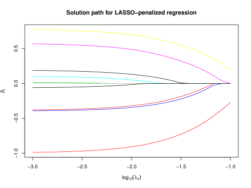
Figure 2: Path plot for LASSO-penalized Fine-Gray regression using our toy example. The tuning parameter $\lambda$ varies between the log-spaced interval $[0.001,0.1]$. The $y$-axis corresponds to the estimated value for $\hat{\beta}_{j}$ and the $x$-axis corresponds to $\lambda$ (on the $\log_{10}$ scale).

Simulation studies

This section provides a more comprehensive illustration of the computational performance of the fastcmprsk package over two popular competing packages cmprsk and crrp. We simulate datasets under various sample sizes and fix the number of covariates $p=100$. We generate the design matrix, $\mathbf{Z}$ from a $p$-dimensional standard normal distribution with mean zero, unit variance, and pairwise correlation $\mbox{corr}(z_{i},z_{j})=\rho^{|i-j|}$, where $\rho=0.5$ simulates moderate correlation. For Section 0.5.1, the vector of regression parameters for cause 1, the cause of interest, is $\bm{\beta}_{1}=(\bm{\beta}^{*},\bm{\beta}^{*},\ldots,\bm{\beta}^{*})$, where $\bm{\beta}^{*}=(0.40,-0.40,0,-0.50,0,0.60,0.75,0,0,-0.80)$. For Section 0.5.2, $\bm{\beta}_{1}=(\bm{\beta}^{*},\mathbf{0}_{p-10})$. We let $\bm{\beta}_{2}=-\bm{\beta}_{1}$. We set $\pi=0.5$, which corresponds to a cause 1 event rate of approximately $41\%$. The average censoring percentage for our simulations varies between $30-35\%$. We use simulateTwoCauseFineGrayModel to simulate these data and average runtime results over 100 Monte Carlo replicates. We report timing on a system with an Intel Core i5 2.9 GHz processor and 16GB of memory.

Comparison to the crr package

In this section, we compare the runtime and estimation performance of the fastCrr function to crr. We vary $n$ from $1,000$ to 500,000 and run fastCrr and crr both with and without variance estimation. We take 100 bootstrap samples, without parallelization, to obtain the bootstrap standard errors with fastCrr. As shown later in the section (Tables 3 and 4), 100 bootstrap samples suffices to produce a good standard error estimate with close-to-nominal coverage for large enough sample sizes in our scenarios. In practice, we recommend users to increase the number of bootstrap samples until the variance estimate becomes stable, when computationally feasible.

Figure 3 depicts how fast the computational complexities of fastCrr (dashed lines) and crr (solid lines) increase as $n$ increases as measured by runtime (in seconds). It shows clearly that the computational complexity of crr increases quadratically ( solid line slopes $\approx 2$) while that of fastCrr is linear ( dashed line slopes $\approx 1$). This implies that the computational gains of fastCrr over crr are expected to grow exponentially as the sample size increases.

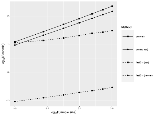
Figure 3: Runtime comparison between fastCrr and crr with and without variance estimation. Axes are on the $\log_{10}$ scale. Solid and dashed lines represent the crrp and fastcmprsk implementation, respectively. Square, and circle symbols denote variance and without variance calculation, respectively. Variance estimation for crr is performed using the asymptotic expression of the variance-covariance estimator. Variance estimation for fastCrr is performed using 100 bootstrap samples. Reported runtime are averaged over 100 Monte Carlo runs.

We further demonstrates the computational advantages of fastCrr over crr for large sample size data in Table 2 by comparing their runtime on a single simulated data with $n$ varying from $50,000$ to $500,000$ using a system with an Intel Xeon 2.40GHz processor and 256GB of memory. It is seen that fastCrr scales well to large sample size data, whereas crr eventually grinds to a halt as $n$ grows large. For example, for $n=500,000$, it only takes less than 1 minute for fastCrr to finish, while crr did not finish in 3 days. Because the forward-backward scan allows us to efficiently compute variance estimates through bootstrapping, we have also observed drastic computational gains in variance estimation with large sample size data (7 minutes for fastCrr versus 54 hours for crr. Furthermore, since parallelization of the bootstrap procedure was not implemented in these timing reports, we expect multicore usage to further decrease the runtime of the variance estimation for fastCrr

Table 2: Runtime comparison of crr versus fasrCrr for large $n$ scenarios. The dashes (“–") indicate that runtime could not be completed within 72 hours. Variance estimation for fastCrr is calculated using $B=100$ bootstrap samples.

	Sample size $n$
	50,000	100,000	500,000
crr without variance	6 hours	24 hours	–
crr with variance	54 hours	–	–
fastCrr without variance	5 seconds	12 seconds	50 seconds
fastCrr with variance	7 minutes	14 minutes	69 minutes

We also performed a simulation to compare the bootstrap procedure for variance estimation to the estimate of the asymptotic variance provided in (3) used in crr. First, we compare the two standard error estimates with the empirical standard error of $\hat{\bm{\beta}}_{1}$. For the $j^{th}$ coefficient, the empirical standard error is calculated as the standard deviation of $\hat{\beta}_{1j}$ from the 100 Monte Carlo runs. For the standard error provided by both the bootstrap and the asymptotic variance-covariance matrix, we take the average standard error of $\hat{\beta}_{1j}$ over the 100 Monte Carlo runs. Table 3 compares the standard errors for $\hat{\beta}_{1j}$ for $j=1,2,3$. When $n=1000$, the average standard error using the bootstrap is slightly larger than the empirical standard error; whereas, the standard error from the asymptotic expression is slightly smaller. These differences diminish and all three estimates are comparable when $n\geq 2000$. This provides evidence that both the bootstrap and asymptotic expression are adequate estimators of the variance-covariance expression for large datasets.

Table 3: Standard error estimates for various different values of $\beta_{1j}$ ($j=1,2,3$). Empirical: Standard deviation of the 100 Monte Carlo estimates of $\hat{\beta}_{1j}$; Bootstrap: The average of the 100 Monte Carlo estimates of the bootstrap standard error for $\hat{\beta}_{1j}$ using $B=100$ bootstrap samples; Asymptotic: The average of 100 Monte Carlo estimates of the standard error estimate for $\hat{\beta}_{1j}$ using the asymptotic variance-covariance matrix defined in (3).

	Std. Err. Est.	$n=$ 1000	2000	3000	4000
$\beta_{11}=0.4$	Empirical	0.06	0.05	0.04	0.03
	Bootstrap	0.10	0.05	0.04	0.03
	Asymptotic	0.07	0.04	0.03	0.03
$\beta_{12}=-0.4$	Empirical	0.10	0.05	0.04	0.03
	Bootstrap	0.11	0.06	0.04	0.04
	Asymptotic	0.08	0.05	0.04	0.03
$\beta_{13}=0$	Empirical	0.09	0.06	0.04	0.03
	Bootstrap	0.11	0.06	0.04	0.04
	Asymptotic	0.07	0.05	0.04	0.03

Additionally, we present in Table 4 the coverage probability (and standard errors) of the $95\%$ confidence intervals for $\beta_{11}=0.4$ using the bootstrap (fastCrr) and asymptotic (crr) variance estimate. The confidence intervals are wider for the bootstrap approach when compared to confidence intervals produced using the asymptotic variance estimator, especially when $n=1000$. However, both methods are close to the nominal $95\%$ level as $n$ increases. We observe similar trends across the other coefficient estimates.

Table 4: Coverage probability (and standard errors) of $95\%$ confidence intervals for $\beta_{11}=0.4$. Confidence intervals for crr are calculated using the asymptotic expression of the variance-covariance estimator. Confidence intervals for fasrCrr are calculated using the bootstrap variance-covariance estimator using 100 bootstrap samples.

	$n$ = 1000	2000	3000	4000
crr	0.93 (0.03)	0.90 (0.03)	0.93 (0.03)	0.95 (0.02)
fastCrr	1.00 (0.00)	0.98 (0.02)	0.95 (0.02)	0.95 (0.02)

Comparison to the crrp package

As mentioned in Section 0.2.4, Fu et al. (2017) provide an R package crrp for performing penalized Fine-Gray regression using the LASSO, SCAD, and MCP penalties. We compare the runtime between fastCrrp with the implementation in the crrp package. To level comparisons, we modify the source code in crrp so that the function only calculates the coefficient estimates and BIC score. We vary $n=1000,1500,\ldots,4000$, fix $p=100$, and employ a 25-value grid search for the tuning parameter. Figure 4 illustrates the computational advantage the fastCrrp function has over crrp.

Similar to the unpenalized scenario, the computational performance of crrp (solid lines) increases quadratically while fasrCrrp (dashed lines) increases linearly, resulting in a 200 to 300-fold speed up in runtime when $n=4000$. This, along with the previous section and a real data analysis conclusion in the following section, strongly suggests that for large-scale competing risks datasets (e.g. EHR databases), where the sample size can easily exceed tens to hundreds of thousands, analyses that may take several hours or days to perform using currently-implemented methods are available within seconds or minutes using our forward-backward scan algorithm.

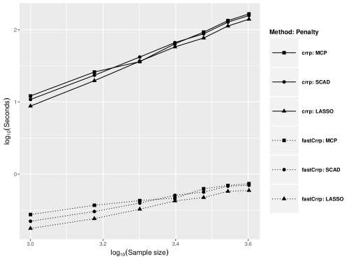
Figure 4: Runtime comparison between the crrp and fastcmprsk implementations of LASSO, SCAD, and MCP penalization. Solid and dashed lines represent the crrp and fastcmprsk implementation, respectively. Square, circle, and triangle symbols denote the penalties MCP, SCAD, and LASSO, respectively. Axes are on the $\log_{10}$ scale. Reported runtime are averaged over 100 Monte Carlo runs.

Discussion

The fastcmprsk package provides a set of scalable tools for the analysis of large-scale competing risks data by developing an approach to linearize the computational complexity required to estimate the parameters of the Fine-Gray proportional subdistribution hazards model. Multicore use is also implemented to further speed up methods that require bootstrapping and resampling. Our simulation results show that our implementation results in a up to 7200-fold decrease in runtime for large sample size data. We also note that in a real-world application, Kawaguchi et al. (2020) record a drastic decrease in runtime ($\approx$ 24 hours vs. $\approx$ 30 seconds) when comparing the proposed implementation of LASSO, SCAD, and MCP to the methods available in crrp on a subset of the United States Renal Data Systems (USRDS) where $n=125,000$. The package implements both penalized and unpenalized Fine-Gray regression and we can conveniently extend our forward-backward algorithm to other applications such as stratified and clustered Fine-Gray regression.

Lastly, our current implementation assumes that covariates are densely observed across subjects. This is problematic in the sparse high-dimensional massive sample size (sHDMSS) domain (Mittal et al., 2014) where the number of subjects and sparsely-represented covariates easily exceed tens of thousands. These sort of data are typical in large comparative effectiveness and drug safety studies using massive administrative claims and EHR databases and typically contain millions to hundreds of millions of patient records with tens of thousands patient attributes, which such settings are particularly useful for drug safety studies of a rare event such as unexpected adverse events (Schuemie et al., 2018) to protect public health. We are currently extending our algorithm to this domain in a sequel paper.

Data generation scheme

We describe the data generation process for the simulateTwoCauseFineGrayModel function. Let $n$, $p$, $\mathbf{Z}_{n\times p}$, $\bm{\beta}_{1}$, $\bm{\beta}_{2}$, $u\mbox{\tiny{min}}$, $u\mbox{\tiny{max}}$ and $\pi$ be specified. We first generate independent Bernoulli random variables to simulate the cause indicator $\epsilon$ for each subject. That is, $\epsilon_{i}\sim 1+Bern\{(1-\pi)^{\exp(\mathbf{z}_{i}^{\prime}\bm{\beta}_{1})}\}$ for $i=1,\ldots,n$. Then, conditional on the cause, event times are simulated from

$$\Pr(T_{i}\leq t|\epsilon_{i}=1,\mathbf{z}_{i}) =\frac{1-[1-\pi\{1-\exp(-t)\}]^{\exp(\mathbf{z}_{i}^{\prime}\bm{\beta}_{1})}}{1-(1-\pi)^{\exp(\mathbf{z}_{i}^{\prime}\bm{\beta}_{1})}}$$

$$\Pr(T_{i}\leq t|\epsilon_{i}=2,\mathbf{z}_{i}) =1-\exp\{-t\exp(\mathbf{z}_{i}^{\prime}\bm{\beta}_{2})\},$$

and $C_{i}\sim U(u\mbox{\tiny{min}},u\mbox{\tiny{max}})$. Therefore, for $i=1,\ldots,n$, we can obtain the following quadruplet $\{(X_{i},\delta_{i},\delta_{i}\epsilon_{i},\mathbf{z}_{i})\}$ where $X_{i}=\min(T_{i},C_{i})$, and $\delta_{i}=I(X_{i}\leq C_{i})$. Below is an excerpt of the code used in simulateTwoCauseFineGrayModel to simulate the observed event times, cause and censoring indicators.

#START CODE.........# nobs, Z, p = pi, u.min, u.max, beta1 and beta2 are already defined.# Simulate cause indicators here using a Bernoulli random variablec.ind <- 1 + rbinom(nobs, 1, prob = (1 - p)^exp(Z %*% beta1))ftime <- numeric(nobs)eta1 <- Z[c.ind == 1, ] %*% beta1 #linear predictor for cause on interesteta2 <- Z[c.ind == 2, ] %*% beta2 #linear predictor for competing risk# Conditional on cause indicators, we simulate the model.u1 <- runif(length(eta1))t1 <- -log(1 - (1 - (1 - u1 * (1 - (1 - p)^exp(eta1)))^(1 / exp(eta1))) / p)t2 <- rexp(length(eta2), rate = exp(eta2))ci <- runif(nobs, min = u.min, max = u.max) # simulate censoring timesftime[c.ind == 1] <- t1ftime[c.ind == 2] <- t2ftime <- pmin(ftime, ci) # X = min(T, C)fstatus <- ifelse(ftime == ci, 0, 1) # 0 if censored, 1 if eventfstatus <- fstatus * c.ind  # 1 if cause 1, 2 if cause 2.........

Eric S. Kawaguchi
University of Southern California
Department of Preventive Medicine
2001 N. Soto St. Los Angeles, CA 90032, USA
eric.kawaguchi@med.usc.edu

Jenny I. Shen
The Lundquist Institute at Harbor-UCLA Medical Center
Division of Nephrology and Hypertension
1124 W. Carson St.
Torrance, CA 90502, USA
jshen@lundquist.org

Gang Li
University of California, Los Angeles
Departments of Biostatistics and Computational Medicine
Los Angeles, CA 90095, USA
vli@ucla.edu

Marc A. Suchard
University of California, Los Angeles
Departments of Biostatistics, Computational Medicine, and Human Genetics
Los Angeles, CA 90095, USA
msuchard@ucla.edu

References

- Akaike (1974) H. Akaike. A new look at the statistical model identification. IEEE Transactions on Automatic Control, 19(6):716–723, 1974.
- Breheny and Huang (2011) P. Breheny and J. Huang. Coordinate descent algorithms for nonconvex penalized regression, with applications to biological feature selection. The Annals of Applied Statistics, 5(1):232, 2011.
- Breslow (1974) N. Breslow. Covariance analysis of censored survival data. Biometrics, 30(1):89–99, 1974. doi: 10.2307/2529620.
- Calaway et al. (2019) R. Calaway, S. Weston, and D. Tenenbaum. doParallel: Foreach Parallel Adaptor for the ’parallel’ Package, 2019. URL https://CRAN.R-project.org/package=doParallel. R package version 1.0.14.
- Cox (1972) D. R. Cox. Regression models and life-tables. Journal of the Royal Statistical Society: Series B (Statistical Methodology), 34(2):187–220, 1972. doi: 10.1007/978-1-4612-4380-9_37.
- Craven and Wahba (1978) P. Craven and G. Wahba. Smoothing noisy data with spline functions. Numerische Mathematik, 31(4):377–403, Dec 1978. ISSN 0945-3245. doi: 10.1007/BF01404567.
- Efron (1979) B. Efron. Bootstrap methods: Another look at the jackknife. The Annals of Statistics, 7(1):1–26, 1979. doi: 10.1214/aos/1176344552.
- Fan and Li (2001) J. Fan and R. Li. Variable selection via nonconcave penalized likelihood and its oracle properties. Journal of the American Statistical Association, 96(456):1348–1360, 2001. doi: 10.1198/016214501753382273.
- Fan and Tang (2013) Y. Fan and C. Y. Tang. Tuning parameter selection in high dimensional penalized likelihood. Journal of the Royal Statistical Society: Series B (Statistical Methodology), 75(3):531–552, 2013. doi: 10.1111/rssb.12001.
- Fine and Gray (1999) J. P. Fine and R. J. Gray. A proportional hazards model for the subdistribution of a competing risk. Journal of the American Statistical Association, 94(446):496–509, 1999. doi: 10.1080/01621459.1999.10474144.
- Fu (2016) Z. Fu. crrp: Penalized Variable Selection in Competing Risks Regression, 2016. URL https://CRAN.R-project.org/package=crrp. R package version 1.0.
- Fu et al. (2017) Z. Fu, C. R. Parikh, and B. Zhou. Penalized variable selection in competing risks regression. Lifetime Data Analysis, 23(3):353–376, 2017. doi: 10.1007/s10985-016-9362-3.
- Gerds et al. (2012) T. A. Gerds, T. H. Scheike, and P. K. Andersen. Absolute risk regression for competing risks: interpretation, link functions, and prediction. Statistics in Medicine, 31(29):3921–3930, 2012. doi: 10.1002/sim.5459.
- Gray (1988) R. J. Gray. A class of k-sample tests for comparing the cumulative incidence of a competing risk. The Annals of Statistics, 16(3):1141–1154, 1988. doi: 10.1214/aos/1176350951.
- Hoerl and Kennard (1970) A. E. Hoerl and R. W. Kennard. Ridge regression: Biased estimation for nonorthogonal problems. Technometrics, 12(1):55–67, 1970. doi: 10.1080/00401706.1970.10488634.
- Kawaguchi et al. (2020) E. S. Kawaguchi, J. I. Shen, M. A. Suchard, and G. Li. Scalable algorithms for large competing risks data. Journal of Computational and Graphical Statistics, accepted pending a minor revision, 2020.
- Kuk and Varadhan (2013) D. Kuk and R. Varadhan. Model selection in competing risks regression. Statistics in Medicine, 32(18):3077–3088, 2013. doi: 10.1002/sim.5762.
- Mittal et al. (2014) S. Mittal, D. Madigan, R. S. Burd, and M. A. Suchard. High-dimensional, massive sample-size cox proportional hazards regression for survival analysis. Biostatistics, 15(2):207–221, 2014. doi: 10.1093/biostatistics/kxt043.
- Ni and Cai (2018) A. Ni and J. Cai. Tuning parameter selection in cox proportional hazards model with a diverging number of parameters. Scandinavian Journal of Statistics, 45(3):557–570, 2018. doi: 10.1111/sjos.12313.
- Robins and Rotnitzky (1992) J. M. Robins and A. Rotnitzky. Recovery of information and adjustment for dependent censoring using surrogate markers. In AIDS epidemiology, pages 297–331. Springer, 1992. doi: 10.1007/978-1-4757-1229-2_14.
- Scheike and Zhang (2011) T. H. Scheike and M.-J. Zhang. Analyzing competing risk data using the r timereg package. Journal of Statistical Software, 38(2), 2011. doi: 10.18637/jss.v038.i02.
- Schuemie et al. (2018) M. J. Schuemie, P. B. Ryan, G. Hripcsak, D. Madigan, and M. A. Suchard. Improving reproducibility by using high-throughput observational studies with empirical calibration. Philosophical Transactions of the Royal Society A: Mathematical, Physical and Engineering Sciences, 376(2128):20170356, 2018. doi: 10.1098/rsta.2017.0356.
- Schwarz (1978) G. Schwarz. Estimating the dimension of a model. The Annals of Statistics, 6(2):461–464, 1978. doi: 10.1214/aos/1176344136.
- Simon et al. (2011) N. Simon, J. Friedman, T. Hastie, and R. Tibshirani. Regularization paths for cox’s proportional hazards model via coordinate descent. Journal of Statistical Software, 39(5):1, 2011.
- Tibshirani (1996) R. Tibshirani. Regression shrinkage and selection via the lasso. Journal of the Royal Statistical Society: Series B (Statistical Methodology), 58(1):267–288, 1996. doi: 10.1.1.35.7574.
- Wang et al. (2007) H. Wang, R. Li, and C.-L. Tsai. Tuning parameter selectors for the smoothly clipped absolute deviation method. Biometrika, 94(3):553–568, 2007. doi: 10.1093/biomet/asm053.
- Wang and Zhu (2011) T. Wang and L. Zhu. Consistent tuning parameter selection in high dimensional sparse linear regression. Journal of Multivariate Analysis, 102(7):1141–1151, 2011. doi: 10.1016/j.jmva.2011.03.007.
- Zhang (2010) C.-H. Zhang. Nearly unbiased variable selection under minimax concave penalty. The Annals of Statistics, 38(2):894–942, 2010. doi: 10.1214/09-aos729.
- Zhang et al. (2010) Y. Zhang, R. Li, and C.-L. Tsai. Regularization parameter selections via generalized information criterion. Journal of the American Statistical Association, 105(489):312–323, 2010. doi: 10.1198/jasa.2009.tm08013.
- Zhou et al. (2011) B. Zhou, A. Latouche, V. Rocha, and J. Fine. Competing risks regression for stratified data. Biometrics, 67(2):661–670, 2011. doi: 10.1111/j.1541-0420.2010.01493.x.
- Zhou et al. (2012) B. Zhou, J. Fine, A. Latouche, and M. Labopin. Competing risks regression for clustered data. Biostatistics, 13(3):371–383, 2012. doi: 10.1093/biostatistics/kxr032.
- Zou (2006) H. Zou. The adaptive lasso and its oracle properties. Journal of the American Statistical Association, 101(476):1418–1429, 2006. doi: 10.1198/016214506000000735.