Alpha MAML: Adaptive Model-Agnostic Meta-Learning

Abstract

Model-agnostic meta-learning (MAML) is a meta-learning technique to train a model on a multitude of learning tasks in a way that primes the model for few-shot learning of new tasks. The MAML algorithm performs well on few-shot learning problems in classification, regression, and fine-tuning of policy gradients in reinforcement learning, but comes with the need for costly hyperparameter tuning for training stability. We address this shortcoming by introducing an extension to MAML, called Alpha MAML, to incorporate an online hyperparameter adaptation scheme that eliminates the need to tune meta-learning and learning rates. Our results with the Omniglot database demonstrate a substantial reduction in the need to tune MAML training hyperparameters and improvement to training stability with less sensitivity to hyperparameter choice.

1 Introduction

Meta-learning—or “learning to learn”—concerns machine learning models that can improve their learning quality by altering aspects of the learning process such as the model architecture, optimization rules, initialization, or learning hyperparameters (Thrun and Pratt, 2012; Schmidhuber, 1987; Hochreiter et al., 2001). An important application of meta-learning is in few-shot learning problems (Vinyals et al., 2016; Behl et al., 2018), where one is concerned with developing methods able to learn new concepts from one or only a few instances (Lake et al., 2015). In this paper we focus on the state-of-the-art model-agnostic meta-learning (MAML) (Finn et al., 2017) method, which is a conceptually simple and general algorithm that has been shown to outperform existing approaches in tasks including few-shot image classification and few-shot adaptation in reinforcement learning (Antoniou et al., 2019). MAML aims to solve the few-shot learning problem by being just few gradient descent steps away from any new concepts, doing so by making the assumption that learning a new concept will just involve few parameter updates (Algorithm 1). In other words, MAML is based on learning an initial representation that can be efficiently fine-tuned for new tasks in a few steps.

The generality of MAML comes with the difficulty of choosing hyperparameters to achieve stable training in practice (Antoniou et al., 2019). MAML has two important hyper-parameters, namely the learning rate $\alpha$ and the meta-learning rate $\beta$, thus increasing any hyperparameter grid search computation by an order, and making it significantly more time and resource consuming than comparable methods. Another complication to this problem is the fact that it is currently not established whether the technique can benefit from a conventional decaying schedule for the inner learning rate $\alpha$. Furthermore, a good value of $\alpha$ in MAML is even more important than for any conventional stochastic gradient descent (SGD) optimization, because only a handful of samples are available in the few-shot learning case. This has significant consequences, making it difficult to scale this algorithm to problems bigger than toy scales, due to the difficulty in assessing whether MAML is not suitable for a complex task or whether the hyperparameters are not sufficiently tuned.

In this paper, we provide a conceptually simple solution to this problem, by introducing an extension of the MAML algorithm to incorporate adaptive tuning of both the learning rate $\alpha$ and the meta-learning rate $\beta$. Our aim is to make it possible to use MAML without or with significantly less parameter tuning, and thus to reduce the need for grid search. We also aim to make the algorithm converge in fewer iterations. The solution we propose is based on the hypergradient descent (HD) algorithm (Baydin et al., 2018), which automatically updates a learning rate by performing gradient descent on the learning rate alongside original optimization steps. The proposed algorithm does not need any extra gradient computations, and just involves storing the gradients from the previous optimization step.

2 Related Work

Our work is primarily related with the subfields of hyperparameter optimization and meta-learning. In hyperparameter optimization one typically uses parallel runs to populate a selected grid of hyperparameter values (e.g., a range of learning rates), or use more advanced techniques such as Bayesian optimization (Snoek et al., 2012) and model-based approaches (Bergstra et al., 2013; Hutter et al., 2013). An interesting line of research, which also inspired our approach in this paper, is to use gradient-based optimization for the tuning of hyperparameters (Bengio, 2000). Recent work in this area include reversible learning (Maclaurin et al., 2015), which allows gradient-based optimization of hyperparameters through a training run consisting of multiple iterations, and hypergradient descent (Baydin et al., 2018), which achieves a similar optimization in an online, per-gradient-update, fashion.

Meta-learning is often referred to as “learning to learn” (Thrun and Pratt, 2012), meaning a learning procedure (most of the time gradient-based) is able to improve aspects of the learning process itself, such as the optimizer, hyperparameters like the learning rate, and initializations. In this sense, the “meta” concept of meta-learning has aspects in common with hyperparameter optimization. The MAML model (Finn et al., 2017) on which we base our method, relies on meta-optimization through gradient descent in a model-agnostic way. Another recent method, Meta-SGD (Li et al., 2017), performs online optimization of a per-parameter learning rate vector $\alpha$, to which the authors refer as learning both the learning rate and update direction (because of the per-parameter nature being able to modify direction), and model parameters $\theta$, using a single hyper-learning rate $\beta$. Our work differs from Meta-SGD as we perform simultaneous online optimization of both MAML learning rates $\alpha$ and $\beta$, which are both scalars.

3 Model-Agnostic Meta-Learning (MAML)

The MAML algorithm, given model parameters $\theta$, aims to adapt to a new task $\mathcal{T}_{t}$ with SGD:

$$\theta_{t}^{\prime}=\theta-\alpha\nabla_{\theta}\mathcal{L}_{\mathcal{T}_{train(t)}}(f_{\theta})\;,$$ (1)

where $t$ is the task number and $\alpha$ is the learning rate. ${T}_{train(t)}$ and ${T}_{test(t)}$ denote the training and test set within task $t$. The tasks are sampled from a defined $p(\mathcal{T})$. The meta-objective is:

$$\min_{\theta}\mathcal{L}_{\mathcal{T}_{test(t)}}(f_{\theta_{t}^{\prime}})=\mathcal{L}_{\mathcal{T}_{test(t)}}(f_{\theta-\alpha\nabla_{\theta}\mathcal{L}_{\mathcal{T}_{train(t)}}(f_{\theta})})$$ (2)

The model aims to optimize the parameters $\theta$ such that with just one SGD step it can adapt to the new task. For the optimization in Eq. 2, this looks as follows:

$$\theta_{t}=\theta-\beta\nabla_{\theta}\mathcal{L}_{\mathcal{T}_{test(t)}}(f_{\theta_{t}^{\prime}})\;,$$ (3)

where $\beta$ is the meta step size. This gives an algorithm that learns an initialization of $\theta$ that is useful for being adapted to new tasks efficiently with a small number of iterations. An important advantage is that this is achieved without making any assumptions on the form of the model. Another advantage is that the meta-learner, introduced in this way based on conventional gradient descent, does not introduce extra model parameters to learn as in model-based approaches in meta-learning. The full algorithm is shown in Algorithm 1. It can be seen that unlike usual SGD which has only one learning rate, MAML has two learning rates $\alpha$ and $\beta$, which require time-consuming hyperparameter tuning.

4 Alpha MAML

Algorithm 1 MAML

  Input: $p(\mathcal{T}):$ distribution over tasks.

  Input: $\alpha,\beta:$ learning rates

  randomly initialize $\theta$.

  while not done do

     Sample batch of tasks $\mathcal{T}_{t}\sim p(\mathcal{T})$

     for all $\mathcal{T}_{t}$  do

        Evaluate $\nabla_{\theta}\mathcal{L}_{\mathcal{T}_{train(t)}}(f_{\theta})$ with respect to $K$ examples.

        Compute adapted parameters with gradient descent: $\theta_{t}^{\prime}=\theta-\alpha\nabla_{\theta}\mathcal{L}_{\mathcal{T}_{train(t)}}(f_{\theta})$

     end for

     Update $\theta=\theta-\beta\nabla_{\theta}\sum_{\mathcal{T}_{t}\sim p(\mathcal{T})}\mathcal{L}_{\mathcal{T}_{test(t)}}(f_{\theta_{t}^{\prime}})$

  end while

Algorithm 2 Alpha MAML

  Input: $p(\mathcal{T}):$ distribution over tasks.

  Input: $\alpha_{0},\beta_{0}:$ initial learning rates

  Input: $\alpha_{\text{hyperlr}},\beta_{\text{hyperlr}}:$ hypergradient learning rates

  randomly initialize $\theta$.

  while not done do

     Sample batch of tasks $\mathcal{T}_{t}\sim p(\mathcal{T})$

     for all $\mathcal{T}_{t}$  do

        Evaluate $\nabla_{\theta}\mathcal{L}_{\mathcal{T}_{train(t)}}(f_{\theta})$ with respect to $K$ examples.

        Compute adapted parameters with gradient descent: $\theta_{t}^{\prime}=\theta-\alpha_{i}\nabla_{\theta}\mathcal{L}_{\mathcal{T}_{train(t)}}(f_{\theta})$

     end for

     $\alpha_{i+1}=\alpha_{i}+\alpha_{\text{hyperlr}}\sum_{\mathcal{T}_{t}\sim p(\mathcal{T})}\nabla_{\theta_{t}^{\prime}}\mathcal{L}_{\mathcal{T}_{test(t)}}(f_{\theta_{t}^{\prime}}).\nabla_{\theta_{i-1}}\mathcal{L}_{\mathcal{T}_{train(t)}}(f_{\theta_{i-1}})$

     $\beta_{i}=\beta_{i-1}+\beta_{\text{hyperlr}}\sum_{\mathcal{T}_{t}\sim p(\mathcal{T})}\nabla_{\theta_{i-1}}\mathcal{L}_{\mathcal{T}_{test(t)}}(f_{\theta_{t}^{\prime}}).\nabla_{\theta_{i-2}}\mathcal{L}_{\mathcal{T}_{test(i-1)}}(f_{\theta_{t}^{\prime}})$

     $\theta_{i}=\theta_{i-1}-\beta_{i}\sum_{\mathcal{T}_{t}\sim p(\mathcal{T})}\nabla_{\theta_{i-1}}\mathcal{L}_{\mathcal{T}_{test(t)}}(f_{\theta_{t}^{\prime}})$

  end while

Eq. 1 is regular gradient descent for adapting to the task $t$, with $\alpha$ being the task-level learning rate. Similarly, Eq. 3 is regular gradient descent for the meta update, with $\beta$ being the meta-learning rate. In addition to the update rules in Equations 1 and 3, we would like to derive update rules for the learning rates $\alpha$ and $\beta$ as well. Our algorithm, Alpha MAML, can simply be written in four update equations as shown in the following derivation. Here $i$ is the iteration number. We first derive the algorithm for the simpler case when each batch has only one task, thus the iteration number is same as the task number $t=i$.

Firstly, our goal is to update the value of $\alpha$ towards the optimum value $\alpha_{i}^{*}$ that minimizes the value of the meta objective Eq. 2 in the next iteration. However, we have not computed $\theta_{i}^{\prime}$ yet. If we assume that the optimal value of $\alpha$ does not change much across iterations, we can estimate it by $\alpha_{i-1}^{*}$. Therefore we perform one gradient descent step over the previous value of learning rate $\alpha_{i-1}$, with gradient:

$$\frac{\partial\mathcal{L}_{\mathcal{T}_{test(i-1)}}(f_{\theta_{i-1}^{\prime}})}{\partial\alpha} =\frac{\partial\mathcal{L}_{\mathcal{T}_{test(i-1)}}(f_{\theta_{i-1}^{\prime}})}{\partial\theta_{i-1}^{\prime}}^{T}\frac{\partial\theta_{i-1}^{\prime}}{\partial\alpha}$$ (4)

$$={\nabla_{\theta_{i-1}^{\prime}}\mathcal{L}_{\mathcal{T}_{test(i-1)}}(f_{\theta_{i-1}^{\prime}})}^{T}$$

$$\;\;\;\;\;\;\;\;\;\frac{\partial(\theta_{i-2}-\alpha_{i-1}\nabla_{\theta_{i-2}}\mathcal{L}_{\mathcal{T}_{train(i-1)}}(f_{\theta_{i-2}}))}{\partial\alpha}$$

$$=\nabla_{\theta_{i-1}^{\prime}}\mathcal{L}_{\mathcal{T}_{test(i-1)}}(f_{\theta_{i-1}^{\prime}}).(-\nabla_{\theta_{i-2}}\mathcal{L}_{\mathcal{T}_{train(i-1)}}(f_{\theta_{i-2}}))$$

We can estimate $\alpha_{i-1}^{*}$ as follows:

$$\alpha_{i}=\alpha_{i-1}+\alpha_{\text{hyperlr}}\nabla_{\theta_{i-1}^{\prime}}\mathcal{L}_{\mathcal{T}_{test(i-1)}}(f_{\theta_{i-1}^{\prime}})\,.\nabla_{\theta_{i-2}}\mathcal{L}_{\mathcal{T}_{train(i-1)}}(f_{\theta_{i-2}})\;,$$ (5)

where $\alpha_{\text{hyperlr}}$ is the hyper learning rate for $\alpha$.

Secondly, we also want to derive an update rule for the meta learning rate $\beta$. Similar to $\alpha$, we would like to update $\beta$ towards its optimal value $\beta_{i}^{*}$ that minimizes the value of the objective $\mathcal{L}_{\mathcal{T}_{test(i)}}(f_{\theta_{i}^{\prime}})$ in the next iteration, making an assumption that the optimal value of $\beta$ does not change much between two consecutive iterations. For this, we compute:

$$\frac{\partial\mathcal{L}_{\mathcal{T}_{test(i)}}(f_{\theta_{i}^{\prime}})}{\partial\beta} =\frac{\partial\mathcal{L}_{\mathcal{T}_{test(i)}}(f_{\theta_{i}^{\prime}})}{\partial\theta_{i-1}}.\frac{\partial\theta_{i-1}}{\partial\beta}$$ (6)

$$=\nabla_{\theta_{i-1}}\mathcal{L}_{\mathcal{T}_{test(i)}}(f_{\theta_{i}^{\prime}}).(-\nabla_{\theta_{i-2}}\mathcal{L}_{\mathcal{T}_{test(i-1)}}(f_{\theta_{i-1}^{\prime}}))$$

We can estimate $\beta_{i-1}^{*}$ as follows:

$$\beta_{i}=\beta_{i-1}+\beta_{\text{hyperlr}}\nabla_{\theta_{i-1}}\mathcal{L}_{\mathcal{T}_{test(i)}}(f_{\theta_{i}^{\prime}}).\nabla_{\theta_{i-2}}\mathcal{L}_{\mathcal{T}_{test(i-1)}}(f_{\theta_{i-1}^{\prime}})\;,$$ (7)

where $\beta_{\text{hyperlr}}$ is the hyper learning rate for $\beta$. It is important to note that in Eq.4 and Eq.6, the gradients are computed with respect to the loss on the test set of a batch. This is done in accordance with the meta-objective. The final Alpha MAML algorithm can thus be written down into just 4 update equations:

$$\theta_{i}^{\prime}=\theta_{i-1}-\alpha_{i}\nabla_{\theta_{i-1}}\mathcal{L}_{\mathcal{T}_{train(i)}}(f_{\theta_{i-1}})$$ (8)

$$\alpha_{i+1}=\alpha_{i}+\alpha_{\text{hyperlr}}\nabla_{\theta_{i}^{\prime}}\mathcal{L}_{\mathcal{T}_{test(i)}}(f_{\theta_{i}^{\prime}}).\nabla_{\theta_{i-1}}\mathcal{L}_{\mathcal{T}_{train(i)}}(f_{\theta_{i-1}})$$

$$\beta_{i}=\beta_{i-1}+\beta_{\text{hyperlr}}\nabla_{\theta_{i-1}}\mathcal{L}_{\mathcal{T}_{test(i)}}(f_{\theta_{i}^{\prime}}).\nabla_{\theta_{i-2}}\mathcal{L}_{\mathcal{T}_{test(i-1)}}(f_{\theta_{i-1}^{\prime}})$$

$$\theta_{i}=\theta_{i-1}-\beta_{i}\nabla_{\theta_{i-1}}\mathcal{L}_{\mathcal{T}_{test(i)}}(f_{\theta_{i}^{\prime}})$$

It can be seen that no extra gradient needs to be computed, as the gradients from the last iteration can be used, requiring only the extra memory storage of the gradient from the previous iteration. The full algorithm with the more general case of multiple tasks in one batch is shown in Algorithm 2. The derivation for this case is shown in the appendix 9.

5 Experiments

To evaluate the performance of Alpha MAML in comparison to MAML, we perform experiments on the few-shot image recognition task on the Omniglot dataset (Lake et al., 2011), which is commonly used in related work (Finn et al., 2017; Ravi and Larochelle, 2017; Snell et al., 2017; Vinyals et al., 2016). We keep the experimentation configuration the same as the original MAML work, for a fair comparison. Omniglot comprises 20 instances (drawn by 20 different people) of 1,623 characters from 50 alphabets. We follow the N-way Omniglot task setup, which was introduced by Vinyals et al. (2016), and also used in MAML (Finn et al., 2017). The N-way classification task is set up as follows: the model is shown K instances from N unseen classes, and then evaluated on some other instances from these N classes. To keep the procedure the same as MAML, we also randomly select 1,200 characters for training, and use the rest for testing. The network architecture follows the architecture used by Finn et al. (2017), and more implementation details are in the appendix A.

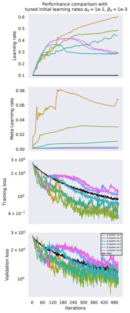
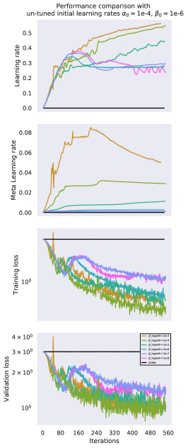
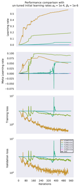
Figure 1: Convergence comparison of Alpha-MAML and MAML, with and without tuned initial learning rate hyper-parameters $\alpha_{0}$ and $\beta_{0}$. Columns: left: tuned initial learning rates; middle: untuned initial learning rates, with varying $\beta_{\text{hyperlr}}$ for Alpha-MAML; right: untuned initial learning rates, with varying $\alpha_{\text{hyperlr}}$ for Alpha-MAML. Rows: first: evolution of the learning rate $\alpha$; second: evolution of the meta learning rate $\beta$; third: training loss; fourth: validation loss.

Behaviour of Alpha MAML vs MAML:

Here we choose a good case (where the MAML user picked a good pair of $\alpha_{0}$ and $\beta_{0}$, i.e., the tuned case) and a bad case (where the user picked a bad pair of $\alpha_{0}$ and $\beta_{0}$, i.e., an untuned case), and plot the evolution of $\alpha_{i}$ and $\beta_{i}$ as a function of iterations, also showing the training and validation losses during training. Figure 1 shows the evolution of learning rate $\alpha_{i}$, meta-learning rate $\beta_{i}$, and the training and validation losses. Results show that even the badly picked $\alpha_{0}$ and $\beta_{0}$ values can be automatically tuned by the online learning rate adaptation scheme in Alpha MAML, tuned in the sense that the algorithm does the necessary adjustments to $\alpha_{i}$ and $\beta_{i}$ in each iteration to achieve a loss similar to the good case. This can be seen in Figure 1 middle and right columns.

Insensitivity with respect to hyperparameter choices:

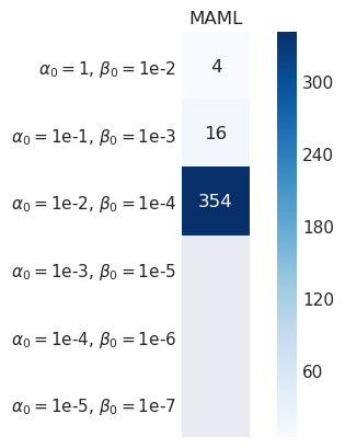
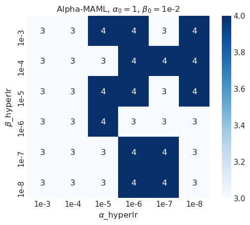
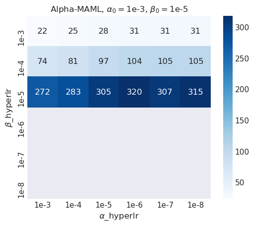
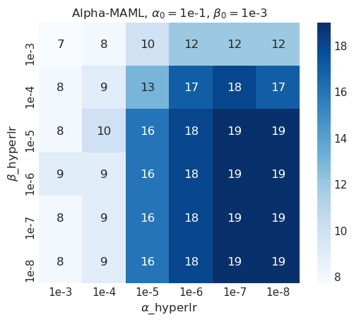
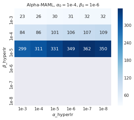
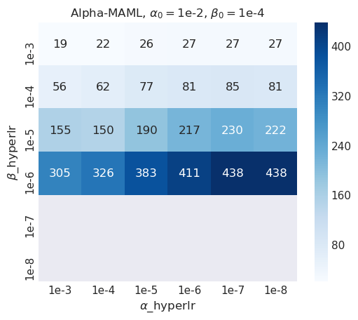
Figure 2: Grid Search for selecting the hyper-parameters in MAML and Alpha-MAML: shows the number of iterations to converge to a training loss of 2.5 for Omniglot dataset. Here the blank cells denote the cases where algorithm did not converge till 500 iterations. It can be seen that as we go far from the tuned hyper-parameter range, converge of Alpha-MAML is better than MAML. Specially for the case of $\alpha_{0}=1e-3,\beta_{0}=1e-5$ Alpha-MAML converged for some cases of $\alpha_{\text{hyperlr}}$ and $\beta_{\text{hyperlr}}$, whereas MAML does not converge till 500 iterations. Same is the case with $\alpha_{0}=1e-4,\beta_{0}=1e-6$, for half of the choices of $\alpha_{\text{hyperlr}}$ and $\beta_{\text{hyperlr}}$, Alpha-MAML converged but MAML does not converge in less than 500 iterations.

Here we run a series of training experiments to study the effect of initial learning rate values on the number of iterations needed for the algorithms to reach a particular chosen loss threshold. Figures 2 and 3 show this grid search for tuning the learning rate hyper-parameters. It can be seen that MAML shows very slow convergence for a range of initial learning rates, more specifically for $\alpha_{0}=1e-4,\beta_{0}=1e-6$ and $\alpha_{0}=1e-5,\beta_{0}=1e-7$. In comparison, Alpha MAML shows comparatively faster convergence for these initial learning rates also, for a wide range of $\alpha_{\text{hyperlr}}$ and $\beta_{\text{hyperlr}}$. For the cases where MAML shows fast convergence, Alpha MAML also shows fast convergence for all values of $\alpha_{\text{hyperlr}}$ and $\beta_{\text{hyperlr}}$. This indicates that in practice no matter which values one chooses for the inital learning and meta-learning rates $\alpha_{0}$ and $\beta_{0}$, Alpha MAML always shows faster, or in the worst case the same, convergence as MAML. In other words, Alpha MAML is less sensitive to the hyperparameter choice as compared to MAML, and hence needs significantly less tuning.

6 Conclusion

Meta-learning is an important and currently relevant approach with potential impact in solving hard problems in computer vision and reinforcement learning. The training instability of meta-learning algorithms as a function of hyperparameter choices is a known shortcoming and currently an active area of research. We have proposed an extension of the state-of-the-art MAML algorithm (Finn et al., 2017) based on the application of the hypergradient descent technique (Baydin et al., 2018) to make MAML training more robust to hyperparameter choices.

A Appendix

We also derive the Alpha MAML update equations for the bigger case of multiple tasks in one batch as follows, where $i$ denotes the iteration number and $t$ is used to denote the task index:

$$\theta_{t}^{\prime}=\theta_{i-1}-\alpha_{i}\nabla_{\theta_{i-1}}\mathcal{L}_{\mathcal{T}_{train(t)}}(f_{\theta_{i-1}})$$ (9)

$$\alpha_{i+1}=\alpha_{i}+\alpha_{\text{hyperlr}}\sum_{\mathcal{T}_{t}\sim p(\mathcal{T})}\nabla_{\theta_{t}^{\prime}}\mathcal{L}_{\mathcal{T}_{test(t)}}(f_{\theta_{t}^{\prime}})\,.\nabla_{\theta_{i-1}}\mathcal{L}_{\mathcal{T}_{train(t)}}(f_{\theta_{i-1}})$$

$$\beta_{i}=\beta_{i-1}+\beta_{\text{hyperlr}}\sum_{\mathcal{T}_{t}\sim p(\mathcal{T})}\nabla_{\theta_{i-1}}\mathcal{L}_{\mathcal{T}_{test(t)}}(f_{\theta_{t}^{\prime}})\,.\nabla_{\theta_{i-2}}\mathcal{L}_{\mathcal{T}_{test(i-1)}}(f_{\theta_{t}^{\prime}})$$

$$\theta_{i}=\theta_{i-1}-\beta_{i}\sum_{\mathcal{T}_{t}\sim p(\mathcal{T})}\nabla_{\theta_{i-1}}\mathcal{L}_{\mathcal{T}_{test(t)}}(f_{\theta_{t}^{\prime}})$$

In the update for $\beta$, the second gradient is the previous step’s gradient.

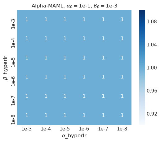
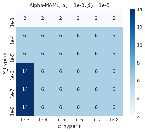
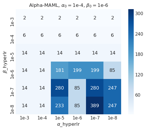
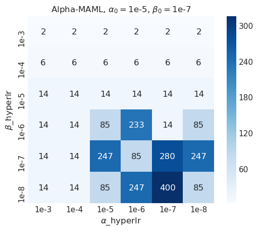
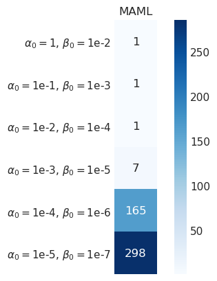
Figure 3: Grid Search for selecting the hyper-parameters in MAML and Alpha-MAML: shows the number of iterations to converge to a training loss of 2.99 for Omniglot dataset. It can be seen that as we go far from the tuned hyper-parameter range, converge of Alpha-MAML is better than MAML. Specially for the case of $\alpha_{0}=1e-4,\beta_{0}=1e-6$ Alpha-MAML converged in less than 15 iterations for a wide range of $\alpha_{\text{hyperlr}}$ and $\beta_{\text{hyperlr}}$, whereas MAML takes 165 iterations. Same is the case with $\alpha_{0}=1e-5,\beta_{0}=1e-7$, for most of the choices of $\alpha_{\text{hyperlr}}$ and $\beta_{\text{hyperlr}}$, Alpha-MAML converged in lesser number of iterations than MAML.

Implementation details

The network has four modules with 3$\times$3 convolutions and 64 filters. This is followed by batch normalization, a ReLU activation, and strided convolutions. The final output is fed into a softmax layer. The images are downsampled to 28$\times$28, and the dimensionality of the last hidden layer is 64.

An augmentation scheme similar to original MAML implementation is applied, where images are augmented with 90 degrees rotated images.

References

- Antoniou et al. (2019) Antreas Antoniou, Harrison Edwards, and Amos Storkey. How to train your MAML. In International Conference on Learning Representations, 2019.
- Baydin et al. (2018) Atılım Güneş Baydin, Robert Cornish, David Martínez Rubio, Mark Schmidt, and Frank Wood. Online learning rate adaptation with hypergradient descent. In Sixth International Conference on Learning Representations (ICLR), Vancouver, Canada, April 30 – May 3, 2018, 2018.
- Behl et al. (2018) Harkirat Singh Behl, Mohammad Najafi, and Philip H. S. Torr. Meta learning deep visual words for fast video object segmentation. CoRR, 2018.
- Bengio (2000) Y. Bengio. Gradient-based optimization of hyperparameters. Neural Computation, 12(8):1889–1900, 2000. doi: 10.1162/089976600300015187.
- Bergstra et al. (2013) J. Bergstra, D. Yamins, and D. D. Cox. Making a science of model search: Hyperparameter optimization in hundreds of dimensions for vision architectures. In International Conference on Machine Learning, 2013.
- Finn et al. (2017) Chelsea Finn, Pieter Abbeel, and Sergey Levine. Model-agnostic meta-learning for fast adaptation of deep networks. In Proceedings of the 34th International Conference on Machine Learning, 2017.
- Hochreiter et al. (2001) Sepp Hochreiter, A Steven Younger, and Peter R Conwell. Learning to learn using gradient descent. In International Conference on Artificial Neural Networks, pages 87–94. Springer, 2001.
- Hutter et al. (2013) F. Hutter, H. Hoos, and K. Leyton-Brown. An evaluation of sequential model-based optimization for expensive blackbox functions. In Proceedings of the 15th Annual Conference Companion on Genetic and Evolutionary Computation, pages 1209–1216. ACM, 2013.
- Lake et al. (2011) Brenden Lake, Ruslan Salakhutdinov, Jason Gross, and Joshua Tenenbaum. One shot learning of simple visual concepts. In Proceedings of the Annual Meeting of the Cognitive Science Society, volume 33, 2011.
- Lake et al. (2015) Brenden M Lake, Ruslan Salakhutdinov, and Joshua B Tenenbaum. Human-level concept learning through probabilistic program induction. Science, 350(6266):1332–1338, 2015.
- Li et al. (2017) Zhenguo Li, Fengwei Zhou, Fei Chen, and Hang Li. Meta-sgd: Learning to learn quickly for few shot learning. CoRR, 2017.
- Maclaurin et al. (2015) D. Maclaurin, D. K. Duvenaud, and R. P. Adams. Gradient-based hyperparameter optimization through reversible learning. In Proceedings of the 32nd International Conference on Machine Learning, pages 2113–2122, 2015.
- Ravi and Larochelle (2017) Sachin Ravi and Hugo Larochelle. Optimization as a model for few-shot learning. In Fifth International Conference on Learning Representations (ICLR), 2017.
- Schmidhuber (1987) Jürgen Schmidhuber. Evolutionary principles in self-referential learning, or on learning how to learn: the meta-meta-… hook. PhD thesis, Technische Universität München, 1987.
- Snell et al. (2017) Jake Snell, Kevin Swersky, and Richard Zemel. Prototypical networks for few-shot learning. In Advances in Neural Information Processing Systems. 2017.
- Snoek et al. (2012) J. Snoek, H. Larochelle, and R. P. Adams. Practical Bayesian optimization of machine learning algorithms. In Advances in Neural Information Processing Systems, pages 2951–2959, 2012.
- Thrun and Pratt (2012) Sebastian Thrun and Lorien Pratt. Learning to learn. Springer Science & Business Media, 2012.
- Vinyals et al. (2016) Oriol Vinyals, Charles Blundell, Tim Lillicrap, koray kavukcuoglu, and Daan Wierstra. Matching networks for one shot learning. In Advances in Neural Information Processing Systems. 2016.