Error analysis for a fractional-derivative parabolic problem on quasi-graded meshes
using barrier functions

Abstract

An initial-boundary value problem with a Caputo time derivative of fractional order $\alpha\in(0,1)$ is considered, solutions of which typically exhibit a singular behaviour at an initial time. For this problem, we give a simple and general numerical-stability analysis using barrier functions, which yields sharp pointwise-in-time error bounds on quasi-graded temporal meshes with arbitrary degree of grading. L1-type and Alikhanov-type discretization in time are considered. In particular, those results imply that milder (compared to the optimal) grading yields optimal convergence rates in positive time. Semi-discretizations in time and full discretizations are addressed. The theoretical findings are illustrated by numerical experiments.

1 Introduction

In this paper we give a simple and general numerical-stability analysis for an initial-boundary value problem with a Caputo time derivative of fractional order $\alpha\in(0,1)$.

• The subtle and sharp stability property (1.2), that we obtain, easily yields sharp pointwise-in-time error bounds for quasi-graded termporal meshes with arbitrary degree of grading. We are not aware of any such general results in the literature.

• In particular, our error bounds accurately predict that milder (compared to the optimal) grading yields optimal convergence rates in positive time. This finding is new, and of practical importance.

• The simplicity of our approach is due to the usage of versatile barrier functions, which can be used in the analysis of any discrete fractional-derivative operator that satisfies the discrete maximum principle (or, more generally, is associated with an inverse-monotone matrix).

• Here this approach is employed in the error analysis of the L1 and Alikhanov L2-1_σ fractional-derivative operators, while in [11] it is used in the analysis of an L2-type discretization of order $3-\alpha$ in time. In [12] this methodology is generalized for semilinear fractional parabolic equations.

The Caputo fractional derivative in time, denoted here by $D_{t}^{\alpha}$, is defined [5] by

$$D_{t}^{\alpha}u(\cdot,t):=\frac{1}{\Gamma(1-\alpha)}\int_{0}^{t}(t-s)^{-\alpha}\,\partial_{s}u(\cdot,s)\,ds\qquad\text{for }\ 0<t\leq T,$$ (1.1)

where $\Gamma(\cdot)$ is the Gamma function, and $\partial_{s}$ denotes the partial derivative in $s$.

Our main stability result is that given an inverse-monotone fractional-derivative operator $\delta_{t}^{\alpha}$, associated with a temporal mesh $\{t_{j}\}_{j=0}^{M}$ on $[0,T]$ with $\tau:=t_{1}$, and $\gamma\in\mathbb{R}$, under certain conditions on the mesh, the following is true for $\{V^{j}\}_{j=0}^{M}$:

$$\left.\begin{array}[]{c}|\delta_{t}^{\alpha}V^{j}|\lesssim(\tau/t_{j})^{\gamma+1}\\[5.69046pt] \forall j\geq 1,\;\;\;V^{0}=0\end{array}\right\}\;\;\Rightarrow\;\;|V^{j}|\lesssim{\mathcal{V}}^{j}:=\tau t_{j}^{\alpha-1}\left\{\begin{array}[]{ll}1&\mbox{if~{}}\gamma>0\\ 1+\ln(t_{j}/\tau)&\mbox{if~{}}\gamma=0\\ (\tau/t_{j})^{\gamma}&\mbox{if~{}}\gamma<0\end{array}\right.\;\;\forall j\geq 1.$$ (1.2)

This result is sharp in the sense that it is consistent with the analogous property for the continuous Caputo operator $D_{t}^{\alpha}$; see Remark 1. The immediate usefulness of this property is due to the fact that truncation errors in time are typically bounded by negative powers of $t_{j}$.

It should be noted that while the explicit inverse of $D_{t}^{\alpha}$ is easily available, the proof of (1.2) for any discrete operator is quite non-trivial. As an alternative, discrete Grönwall inequalities were recently employed in the error analysis of L1- and Alikhanov-type schemes [13, 14, 15]. However, this approach involves intricate evaluations and, furthermore, yields less sharp error bounds (see Remarks 10 and 25 for a more detailed discussion). Our approach is entirely different and is substantially more concise as we obtain (1.2) using clever barrier functions, while the numerical results indicate that our error bounds are sharp in the pointwise-in-time sense.

The following fractional-order parabolic problem is considered:

$$\begin{array}[]{l}D_{t}^{\alpha}u+{\mathcal{L}}u=f(x,t)\quad\mbox{for}\;\;(x,t)\in\Omega\times(0,T],\\[5.69046pt] u(x,t)=0\quad\mbox{for}\;\;(x,t)\in\partial\Omega\times(0,T],\qquad u(x,0)=u_{0}(x)\quad\mbox{for}\;\;x\in\Omega.\end{array}$$ (1.3)

This problem is posed in a bounded Lipschitz domain $\Omega\subset\mathbb{R}^{d}$ (where $d\in\{1,2,3\}$). The spatial operator ${\mathcal{L}}$ here is a linear second-order elliptic operator:

$${\mathcal{L}}u:=\sum_{k=1}^{d}\Bigl{\{}-\partial_{x_{k}}\!(a_{k}(x,t)\,\partial_{x_{k}}\!u)+b_{k}(x,t)\,\partial_{x_{k}}\!u\Bigr{\}}+c(x,t)\,u,$$ (1.4)

with sufficiently smooth coefficients $\{a_{k}\}$, $\{b_{k}\}$ and $c$ in $C(\bar{\Omega})$, for which we assume that $a_{k}>0$ in $\bar{\Omega}$, and also either $c\geq 0$ or $c-\frac{1}{2}\sum_{k=1}^{d}\partial_{x_{k}}\!b_{k}\geq 0$.

The first part of the paper is devoted to L1-type schemes for problem (1.3), which employ the discetization of $D^{\alpha}_{t}u$ defined, for $m=1,\ldots,M$, by

$$\delta_{t}^{\alpha}U^{m}:=\frac{1}{\Gamma(1-\alpha)}\sum_{j=1}^{m}\delta_{t}U^{j}\!\int_{t_{j-1}}^{t_{j}}\!\!(t_{m}-s)^{-\alpha}\,ds,\qquad\delta_{t}U^{j}:=\frac{U^{j}-U^{j-1}}{t_{j}-t_{j-1}},\vspace{-0.1cm}$$ (1.5)

when associated with the temporal mesh $0=t_{0}<t_{1}<\ldots<t_{M}=T$ on $[0,T]$. The generality of our approach is demonstrated in the second part of the paper by extending the stability and error analysis to higher-order Alikhanov-type schemes [1].

Similarly to [2, 3, 4, 10, 13, 14, 16, 17, 20], our main interest will be in graded temporal meshes as they offer an efficient way of computing reliable numerical approximations of solutions singular at $t=0$, which is typical for (1.3). In particular, [4, 10, 17, 20] give global-in-time error bounds on graded meshes for problems of type (1.3) for the L1 method [20, 10], the Alikhanov method [4], and a high-order Petrov-Galerkin method in time [17]. There is also a lot of interest in the literature in optimal error bounds in positive time on uniform meshes; see, e.g., [6, 8, 9, 10].

• By contrast, here, as well as in the related paper [11], pointwise-in-time error bounds will be obtained, while an arbitrary degree of mesh grading (with uniform meshes included as a particular case) is allowed.

• More general temporal meshes, which may be viewed as obtained by adding new nodes in an arbitrary manner to a quasi-graded mesh, are also considered; see Section 2.4 and Theorems 9 and 14.

• For both considered discretizations, when the optimal grading parameter $r=(p-\alpha)/\alpha$ is used, we recover the optimal global convergence rates of $p-\alpha$, where $p=2$ for the L1 scheme and $p=3$ for the Alikhanov scheme, as particular cases of our more general error bounds; see Remarks 11 and 20.

• Another straightforward particular case of our error bounds indicates that the optimal convergence rates $p-\alpha$ in positive time $t\gtrsim 1$ are attained using much milder grading with $r>p-\alpha$; see Remarks 10 and 19. The accuracy of these threshold values is demonstrated by the numerical results in §§5.3–5.4.

• When dealing with the fractional parabolic case, for L1-type schemes we follow [10], while for Alikhanov-type schemes, our approach substantially differs from [1, 4] (as we aim at pointwise-in-time error bounds), so we build on some ideas from [11], which may be of independent interest.

• In the latter case, a much milder grading with $r=2$ (compared to the optimal $r=2/\alpha$) yields the optimal convergence order $2$; see Remark 25.

Throughout the paper, it is assumed that there exists a unique solution of this problem such that $\|\partial_{t}^{l}u(\cdot,t)\|_{L_{2}(\Omega)}\lesssim 1+t^{\alpha-l}$ for $l\leq 3$. This is a realistic assumption, satisfied by typical solutions of problem (1.3) (see, e.g., [18], [20, §2], [10, §6]), in contrast to stronger assumptions of type $\|\partial^{l}u(\cdot,t)\|_{L_{2}(\Omega)}\lesssim 1$ frequently made in the literature (see, e.g., references in [7, Table 1.1]). Indeed, [19, Theorem 2.1] shows that if a solution $u$ of (1.3) is less singular than we assume, then the initial condition $u_{0}$ is uniquely defined by the other data of the problem, which is clearly too restrictive. At the same time, our results can be easily applied to the case of $u$ having no singularities or exhibiting a somewhat different singular behaviour at $t=0$.

Remark 1.

The stability result (1.2) is sharp in the sense that it is consistent with the analogous property for the continuous Caputo operator $D_{t}^{\alpha}$. Indeed, a calculation shows that if $v(0)=0$ and $D_{t}^{\alpha}v(t)=F(t):=\min\{1,(\tau/t)^{\gamma+1}\}$ for $t>0$, then the explicit representation $v(t)=J^{\alpha}_{t}F(t)=\{\Gamma(\alpha)\}^{-1}\!\!\int_{0}^{t}(t-s)^{\alpha-1}F(s)\,ds$ yields $v(t)\simeq{\mathcal{V}}(t)$ for $t\geq\tau$, where ${\mathcal{V}}(t)$ is a continuous version of ${\mathcal{V}}^{j}$ from (1.2).

Outline. §2 is devoted to the proof of the stability result (1.2) for the L1 discrete fractional-derivative operator. This result is then employed in §3 to obtain pointwise-in-time error bounds for L1-type discretizations of the initial-value problem in §3.1, as well as semi-discretizations and full discretizations of the initial-boundary-value problems in §3.2 and §3.3. The above error analysis is extended to the Alikhanov-type discretizations in §4. Finally, our theoretical findings are illustrated by numerical experiments in §5.

Notation. We write $a\simeq b$ when $a\lesssim b$ and $a\gtrsim b$, and $a\lesssim b$ when $a\leq Cb$ with a generic constant $C$ depending on $\Omega$, $T$, $u_{0}$ and $f$, but not on the total numbers of degrees of freedom in space or time. Also, for $1\leq p\leq\infty$, and $k\geq 0$, we shall use the standard norms in the spaces $L_{p}(\Omega)$ and the related Sobolev spaces $W_{p}^{k}(\Omega)$, while $H^{1}_{0}(\Omega)$ is the standard space of functions in $W_{2}^{1}(\Omega)$ vanishing on $\partial\Omega$.

2 Stability properties of the L1 discrete fractional-derivative operator

2.1 Quasi-graded temporal meshes. Main stability result

Throughout the paper, we shall frequently assume that the temporal mesh is quasi-graded in the sense that, with some $r\geq 1$,

$$\tau:=t_{1}\simeq M^{-r},\quad t_{j}\simeq\tau j^{r},\quad\tau_{j}:=t_{j}-t_{j-1}\simeq\tau^{1/r}t_{j}^{1-1/r}\quad\forall\,j=1,\ldots,M.$$ (2.1)

For example, the standard graded temporal mesh $\{t_{j}=T(j/M)^{r}\}_{j=0}^{M}$ with some $r\geq 1$ (while $r=1$ generates a uniform mesh) satisfies (2.1), in view of $\tau_{j}\simeq M^{-1}\,t_{j-1}^{1-1/r}$ and $t_{j}\leq 2^{r}t_{j-1}$ for $j\geq 2$.

Furthermore, our results also apply to more general meshes that may be viewed as obtained by adding new nodes to any mesh of type (2.1); see Section 2.4.

The key in our error analysis for L1-type discretizations is the following stability property.

Theorem 2 (Stability).

(i) Let the temporal mesh satisfy (2.1) with $1\leq r\leq(2-\alpha)/\alpha$. Given $\gamma\in\mathbb{R}$ and $\{V^{j}\}_{j=0}^{M}$, the stability property (1.2) holds true.
(ii) If $\gamma\leq\alpha-1$, then (1.2) holds true on an arbitrary temporal mesh $\{t_{j}\}_{j=0}^{M}$.
(iii) The above results remain valid if $|\delta_{t}^{\alpha}V^{j}|\lesssim(\tau/t_{j})^{\gamma+1}$ in (1.2) is replaced by $\delta_{t}^{\alpha}|V^{j}|\lesssim(\tau/t_{j})^{\gamma+1}$.

Proof.

(i) It suffices to prove part (i) only for $\gamma\geq\alpha-1$ (as the result of part (ii) applies to the case $\gamma\leq\alpha-1$). The proof is presented in Sections 2.2 and 2.3, where a few cases are considered separately.

(ii) This result is easily obtained from [10, Lemma 2.1(i)]. The latter implies that $|V^{m}|\lesssim\max_{j\leq m}\bigl{\{}t_{j}^{\alpha}|\delta_{t}^{\alpha}V^{j}|\bigr{\}}$ on an arbitrary mesh. The assumptions on $\{V^{j}\}$ yield $t_{j}^{\alpha}|\delta_{t}^{\alpha}V^{j}|\lesssim t_{j}^{\alpha}(\tau/t_{j})^{\gamma+1}=\tau^{\gamma+1}t_{j}^{\alpha-\gamma-1}$, which, combined with $\gamma\leq\alpha-1$, implies $t_{j}^{\alpha}|\delta_{t}^{\alpha}V^{j}|\lesssim\tau^{\gamma+1}t_{m}^{\alpha-\gamma-1}$ $\forall\,j\leq m$. The desired assertion $|V^{m}|\lesssim\tau^{\gamma+1}t_{m}^{\alpha-\gamma-1}$ follows.

(iii) Imitate the proof of [10, Lemma 2.1(ii)]. To be more precise, let $W^{0}=0$ and $\delta_{t}^{\alpha}W^{j}=\max\bigl{\{}0,\,\delta_{t}^{\alpha}|V^{j}|\bigr{\}}\geq\delta_{t}^{\alpha}|V^{j}|$ $\forall\,j\geq 1$. Then $0\leq|V^{j}|\leq W^{j}$ $\forall\,j\geq 1$ (as $\delta_{t}^{\alpha}$ is associated with an $M$-matrix), while the results of parts (i) and (ii) apply to $\{W^{j}\}$. ∎

Remark 3.

To a degree, the proof of Theorem 2 builds on the analysis in [10, Appendix A] for uniform grids, but now we address considerably more general meshes.

2.2 Proof of Theorem 2(i) for $\gamma\geq\alpha$

In this case $(\tau/t_{j})^{\gamma+1}\leq(\tau/t_{j})^{\alpha+1}$, so it suffices to consider only $\gamma=\alpha$. For the latter case, as the operator $\delta_{t}^{\alpha}$ is associated with an $M$-matrix, it suffices to prove the following lemma.

Lemma 4.

Let the temporal mesh satisfy (2.1) with $1\leq r\leq(2-\alpha)/\alpha$. Then there exists a discrete barrier function $\{B^{j}\}_{j=0}^{M}$ such that

$$B^{0}=0,\qquad 0\leq B^{j}\lesssim t_{j}^{\alpha-1},\qquad\delta_{t}^{\alpha}B^{j}\gtrsim\tau^{\alpha}t_{j}^{-\alpha-1}\qquad\forall j\geq 1.$$ (2.2)

Proof.

Fix a sufficiently large number $2\leq p\lesssim 1$, and then set

$$\beta:=1-\alpha,\qquad B(s):=\min\bigl{\{}(s/t_{p})t_{p}^{-\beta},s^{-\beta}\bigr{\}},\qquad B^{j}:=B(t_{j}).$$ (2.3)

Note that, when using the notation of type $\lesssim$, the dependence on $p$ will be shown explicitly.

For $j\leq p$, a straightforward calculation shows that $\delta_{t}^{\alpha}B^{j}=D^{\alpha}_{t}B(t_{j})\simeq t_{j}^{\beta}t_{p}^{-\beta-1}\simeq p^{-r(2-\alpha)}t_{j}^{\beta}\tau^{-\beta-1}$, where we also used $t_{p}\simeq\tau p^{r}$ (in view of (2.1)). As $t_{j}\geq\tau$, we then get $\delta_{t}^{\alpha}B^{j}\gtrsim p^{-r(2-\alpha)}\tau^{-\beta}t_{j}^{\beta-1}\geq p^{-r(2-\alpha)}\tau^{\gamma}t_{j}^{-\gamma-1}$ $\forall\gamma\geq\alpha-1$ including $\gamma=\alpha$.

Next, for $D_{t}^{\alpha}B(t)$ with $t>t_{p}$ one has

$$\Gamma(1-\alpha)\,D^{\alpha}_{t}B(t)= \underbrace{\int_{0}^{t_{p}}\!\!t_{p}^{-\beta-1}(t-s)^{-\alpha}\,ds}_{{}\geq t_{p}^{-\beta}t^{-\alpha}}-\underbrace{\beta\int_{t_{p}}^{t}\!s^{-\beta-1}(t-s)^{-\alpha}\,ds}_{{}=:t^{-1}{I}}\,.$$

Here, using $\hat{s}:=s/t$ and $\hat{t}_{p}:=t_{p}/t$, and noting that $\alpha+\beta=1$, one gets

$${I}=\beta\int_{\hat{t}_{p}}^{1}\hat{s}^{-\beta-1}(1-\hat{s})^{-\alpha}\,d\hat{s}=\hat{t}_{p}^{-\beta}(1-\hat{t}_{p})^{\beta}\leq\hat{t}_{p}^{-\beta}(1-\beta\hat{t}_{p}).$$

Now, using $t^{-1}\hat{t}_{p}^{-\beta}=t_{p}^{-\beta}t^{-\alpha}$, one concludes that

$$\Gamma(1-\alpha)\,D^{\alpha}_{t}B(t)\geq t_{p}^{-\beta}t^{-\alpha}\,(\beta t_{p}/t)=\beta t_{p}^{\alpha}t^{-\alpha-1}\qquad\mbox{for}\;\;t>t_{p}.$$ (2.4)

So, to complete the proof, it remains to show that $|\delta^{\alpha}_{t}B^{m}-D^{\alpha}_{t}B(t_{m})|\leq\frac{1}{2}D^{\alpha}_{t}B(t_{m})$ for any $m>p$.

For the latter, note that $\Gamma(1-\alpha)[\delta^{\alpha}_{t}B^{m}-D^{\alpha}_{t}B(t_{m})]=\sum_{j=1}^{m}\mu^{j}$, where, using the standard piecewise-linear interpolant $B^{I}$ of $B$,

$$\mu^{j}:=\int_{t_{j-1}}^{t_{j}}\!\!(B^{I}-B)^{\prime}(s)\,(t_{m}-s)^{-\alpha}ds=\alpha\int_{t_{j-1}}^{t_{j}}\!\!(B-B^{I})(s)\,(t_{m}-s)^{-\alpha-1}ds.$$ (2.5)

Clearly, $\mu^{j}=0$ for $j\leq p$. For $p+1\leq j\leq m-1$, one gets $|B-B^{I}|\lesssim\tau_{j}^{2}|B^{\prime\prime}(t_{j-1})|$. For $j=m$, we shall use a similar, but sharper bound $|B-B^{I}|\lesssim\tau_{j}(t_{m}-s)|B^{\prime\prime}(t_{j-1})|$. Combining these yields $|B-B^{I}|\leq\tau^{2}_{j}\min\bigl{\{}1,(t_{m}-s)/\tau_{m}\bigr{\}}|B^{\prime\prime}(t_{j-1})|$ for $j>p$, where $|B^{\prime\prime}(t_{j-1})|\lesssim|B^{\prime\prime}(s)|\simeq s^{-\beta-2}$ (in view of $t_{j-1}\simeq t_{j}$). Also noting that, in view of (2.1), $\tau_{j}\simeq\tau^{1/r}t_{j}^{1-1/r}\simeq\tau^{1/r}s^{1-1/r}$, we arrive at

$$|\mu^{j}|\lesssim\tau^{2/r}\!\int_{t_{j-1}}^{t_{j}}\!\!\!s^{-\beta-2/r}\,(t_{m}-s)^{-\alpha-1}\,\min\bigl{\{}1,(t_{m}-s)/\tau_{m}\bigr{\}}\,ds\qquad\forall\,p>m.$$

This immediately yields the bound

$$\left|\delta^{\alpha}_{t}B^{m}-D^{\alpha}_{t}B(t_{m})\right|\lesssim\tau^{2/r}\!\int_{t_{p}}^{t_{m}}\!\!\!s^{-\beta-2/r}\,(t_{m}-s)^{-\alpha-1}\,\min\bigl{\{}1,(t_{m}-s)/\tau_{m}\bigr{\}}\,ds.$$ (2.6)

For the latter, using the substitution $s=t_{m}\hat{s}$ and the notation $\hat{t}_{j}:=t_{j}/t_{m}$, $\hat{\tau}_{j}:=\tau_{j}/t_{m}$, one gets

$$\left|\delta^{\alpha}_{t}B^{m}-D^{\alpha}_{t}B(t_{m})\right|\lesssim\tau^{2/r}t_{m}^{-2/r-1}\underbrace{\int_{\hat{t}_{p}}^{1}\!\hat{s}^{-\beta-2/r}(1-\hat{s})^{-\alpha-1}\min\bigl{\{}1,(1-\hat{s})/\hat{\tau}_{m}\bigr{\}}\,d\hat{s}}_{\lesssim\,\hat{t}_{p}^{\alpha-2/r}+\hat{\tau}_{m}^{-\alpha}}.$$

Here, when bounding the integral, it is convenient to separately consider the intervals $(\hat{t}_{p},\max\{\frac{1}{2},\hat{t}_{p}\})$, $(\max\{\frac{1}{2},\hat{t}_{p}\},1-\hat{\tau}_{m})$ and $(1-\hat{\tau}_{m},1)$, where $\hat{\tau}_{m}\leq\frac{1}{2}$ if $p$ is sufficiently large (as, in view of (2.1), $\hat{\tau}_{m}\simeq 1/m\leq 1/p$). On these three intervals, the integrand is respectively $\lesssim s^{-\beta-2/r}$, $\lesssim(t_{m}-s)^{-\alpha-1}$ and $\lesssim(t_{m}-s)^{-\alpha}/\tau_{m}$, so the corresponding integrals are respectively $\lesssim\hat{t}_{p}^{\alpha-2/r}$, $\lesssim\hat{\tau}_{m}^{-\alpha}$ and $\lesssim\hat{\tau}_{m}^{-\alpha}$. Finally, note that $\hat{\tau}_{m}=\tau_{m}/t_{m}\simeq(\tau/t_{m})^{1/r}$, while, in view of $r\leq(2-\alpha)/\alpha$, one has $(\tau/t_{m})^{(2-\alpha)/r}\lesssim(\tau/t_{m})^{\alpha}$. Now, a calculation shows that

$$\left|\delta^{\alpha}_{t}B^{m}-D^{\alpha}_{t}B(t_{m})\right| \lesssim\tau^{2/r}t_{m}^{-2/r-1}\Bigl{[}(t_{p}/t_{m})^{\alpha-2/r}+(\tau/t_{m})^{-\alpha/r}\Bigr{]}$$

$$\lesssim(\tau/t_{p})^{2/r}t_{p}^{\alpha}t_{m}^{-\alpha-1}+\underbrace{t_{m}^{-1}(\tau/t_{m})^{(2-\alpha)/r}}_{\lesssim\tau^{\alpha}t_{m}^{-\alpha-1}}$$

$$\lesssim\Bigl{[}(\tau/t_{p})^{2/r}+(\tau/t_{p})^{\alpha}\Bigr{]}\,t_{p}^{\alpha}t_{m}^{-\alpha-1}.$$ (2.7)

Combining this with (2.4) and choosing $p$ sufficiently large yields the desired assertion $\delta^{\alpha}_{t}B^{m}\gtrsim t_{p}^{\alpha}t_{m}^{-\alpha-1}$ $\forall\,m>p$, and hence $\forall\,m\geq 1$. ∎

Corollary 5.

Lemma 4 remains valid if the temporal mesh is obtained by adding new nodes to any mesh of type (2.1) under the condition that the first mesh interval remains unchanged.

Proof.

Suppose the temporal mesh $\{t_{k}^{\prime}\}$ is obtained by refining the mesh $\{t_{j}\}_{j=0}^{M}$ of type (2.1). For $t_{k}^{\prime}\leq t_{p}$, it is essential that $t_{1}^{\prime}=t_{1}=\tau$, so the desired result is obtained exactly as in the proof of Lemma 4. For $t_{k}^{\prime}>t_{p}$, the desired result is obtained by combining (2.4) with the bound $|D^{\alpha}_{t}(B^{I}-B)|\leq\frac{1}{2}D^{\alpha}_{t}B$ at any $t_{k}^{\prime}>t_{p}$, where $B^{I}$ denotes the piecewise-linear interpolant on the new mesh $\{t_{k}^{\prime}\}$. If $t_{k}^{\prime}=t_{m}$ for some $m>p$, we again proceed exactly as in the proof of Lemma 4, as the same bounds on $B-B^{I}$ hold true (even though $B^{I}$ is now the interpolant on a finer mesh). If $t_{k}^{\prime}\in(t_{m},t_{m+1})$ for $m\geq p$, then on $(t_{m-1},t_{k}^{\prime})$ one employs $|B-B^{I}|\lesssim\tau_{m}(t_{k}^{\prime}-s)|B^{\prime\prime}(t_{m-1})|\lesssim\tau_{m}^{2}\min\{1,\,(t_{k}^{\prime}-s)/\tau_{m}\}|B^{\prime\prime}(t_{m-1})|$. Hence, one gets a version of (2.6) with $t_{m}$ replaced by $t_{k}^{\prime}$, which (in view of $t_{k}^{\prime}\simeq t_{m}$) leads to the desired version of (2.7) at $t_{k}^{\prime}$. ∎

2.3 Proof of Theorem 2(i) for $\gamma<\alpha$

We shall use the notation and some findings from the proof of Lemma 4. In particular, $\beta=1-\alpha$, while $p\simeq 1$ was chosen sufficiently large in the proof of Lemma 4. When using the notation of type $\lesssim$, the dependence on $\gamma$ and $m$, but not on $p$, will be shown explicitly.

For $m\geq 0$ and $\gamma<\alpha$, set

$$p_{m}:=2^{m}p,\qquad B_{m}^{j}:=\min\bigl{\{}t_{j}t_{p_{m}}^{-\beta-1},t_{j}^{-\beta}\bigr{\}},\qquad c_{m}:=2^{-m\gamma r}\;\;\Rightarrow\;\;c_{m}t_{p_{m}}^{\gamma}\simeq\tau^{\gamma}.$$ (2.8)

Here the final observation follows from (2.1) (which yields $t_{p_{m}}\simeq\tau p_{m}^{r}$).

Note that $B_{0}^{j}=B^{j}$, and, more generally, $B_{m}^{j}=B^{j}\big{|}_{p:=p_{m}}$, where $B^{j}$ is from (2.3). Conveniently, in the proof of Lemma 4, the dependance on any sufficiently large $p$ was shown explicitly. In particular, we recall that $\delta_{t}^{\alpha}B_{m}^{j}\geq 0$ for $j\geq 0$. Furthermore,

$$\delta_{t}^{\alpha}B_{0}^{j}\gtrsim\tau^{\gamma}t_{j}^{-\gamma-1}\;\;\mbox{for}\;1\leq j\leq p_{0},\qquad c_{m}(\delta_{t}^{\alpha}B_{m}^{j})\gtrsim\tau^{\gamma}t_{j}^{-\gamma-1}\;\;\mbox{for}\;p_{m}<j\leq p_{m+1}.$$ (2.9)

The first relation for $B_{0}^{j}=B^{j}$ can be found in the above-mentioned proof for $\gamma\geq\alpha-1$ (but is, in fact, valid for any fixed $\gamma$ now that the dependence on $p$ is inessential). The second relation in (2.9) follows from the bound of type (2.4) also obtained there: $\delta^{\alpha}_{t}B^{j}_{m}\gtrsim t_{p_{m}}^{\alpha}t_{j}^{-\alpha-1}$. The latter, indeed, implies $c_{m}(\delta_{t}^{\alpha}B_{m}^{j})\gtrsim c_{m}t_{p_{m}}^{\gamma}t_{j}^{-\gamma-1}\simeq\tau^{\gamma}t_{j}^{-\gamma-1}$ for $p_{m}<j\leq p_{m+1}$ (also using the final bound in (2.8)).

Now we are prepared to prove the following two lemmas, which are sufficient for establishing Theorem 2(i) for $\gamma\in(0,\alpha)$ and $\gamma\leq 0$ respectively.

Lemma 6.

Under the conditions of Theorem 2(i), suppose that $\gamma\in(0,\alpha)$. Then there exists a discrete barrier function $\{\bar{B}^{j}\}_{j=0}^{M}$ such that $\bar{B}^{0}=0$, while $0\leq\bar{B}^{j}\lesssim t_{j}^{\alpha-1}$ and $\delta_{t}^{\alpha}\bar{B}^{j}\gtrsim\tau^{\gamma}t_{j}^{-\gamma-1}$ for $j\geq 1$.

Proof.

Using (2.8), let $\bar{B}^{j}:=\sum_{m=0}^{\infty}c_{m}B_{m}^{j}$. Then $\delta_{t}^{\alpha}\bar{B}^{j}\gtrsim\tau^{\gamma}t_{j}^{-\gamma-1}$ $\forall j\geq 1$ follows from (2.9), while $\sum_{m=0}^{\infty}c_{m}=C_{\gamma}:=(1-2^{-\gamma r})^{-1}$, so $\bar{B}^{j}\leq C_{\gamma}t_{j}^{-\beta}=C_{\gamma}t_{j}^{\alpha-1}$, which completes the proof. ∎

Lemma 7.

Under the conditions of Theorem 2(i), suppose that $\gamma\in[\alpha-1,0]$. If $V^{0}=0$ and $|\delta_{t}^{\alpha}V^{j}|\lesssim\tau^{\gamma}t_{j}^{-\gamma-1}$ for $j=1,\ldots,n\leq M$, then $|V^{n}|\lesssim t_{n}^{\alpha-1}[1+\ln(t_{n}/\tau)]$ if $\gamma=0$, and $|V^{n}|\lesssim t_{n}^{\alpha-1}(\tau/t_{n})^{\gamma}$ if $\gamma\leq 0$.

Proof.

Using (2.8), let $\bar{B}^{j}:=\sum_{m=0}^{N}c_{m}B_{m}^{j}$, where $N=0$ if $n\leq p$, and $N:=\lceil\log_{2}(n/p)-1\rceil$ otherwise, so that $p_{N}<n\leq p_{N+1}$. Note also that $N\lesssim\ln n\simeq\ln(t_{n}/\tau)$ (as $t_{n}/\tau\simeq n^{r}$ in view of (2.1)). Then $\delta_{t}^{\alpha}\bar{B}^{j}\gtrsim\tau^{\gamma}t_{j}^{-\gamma-1}$ for $1\leq j\leq n$ follows from (2.9). Hence $|V^{j}|\lesssim\bar{B}^{j}$ $\forall j\leq n$, in particular $|V^{n}|\lesssim\bar{B}^{n}$.

On the other hand, $\bar{B}^{n}\leq t_{n}^{\alpha-1}\sum_{m=0}^{N}c_{m}$. When $\gamma=0$, each $c_{m}=1$, so $\sum_{m=0}^{N}c_{m}=1+N\simeq 1+\ln(t_{n}/\tau)$, so, indeed, $\bar{B}^{n}\leq t_{n}^{\alpha-1}[1+\ln(t_{n}/\tau)]$. When $\gamma\in[\alpha-1,0)$, we get $\sum_{m=0}^{N}c_{m}=(c_{N+1}-1)/(c_{1}-1)$, where $c_{N+1}\simeq(\tau/t_{p_{N+1}})^{\gamma}\simeq(\tau/t_{n})^{\gamma}$, while $C_{\gamma}:=(c_{1}-1)^{-1}=(2^{|\gamma|r}-1)^{-1}$, so finally $|V^{n}|\lesssim\bar{B}^{n}\lesssim C_{\gamma}t_{n}^{\alpha-1}(\tau/t_{n})^{\gamma}$. ∎

2.4 More general temporal meshes

Our main stability result, Theorem 2, remains valid for more general temporal meshes that may be viewed as obtained by adding new nodes to any mesh of type (2.1) under the condition that the first mesh interval remains unchanged. Indeed, an inspection of the proof of Corollary 5 reveals that not only Lemma 4, but also the results of Section 2.3 are valid for the above temporal mesh. Such more general meshes may be useful if the solution exhibits additional singularities away from the initial time.

Lemma 8.

Theorem 2 remains valid if the temporal mesh satisfies the following weaker version of (2.1):

$$\tau:=t_{1}\simeq M^{-r},\qquad\tau_{j}:=t_{j}-t_{j-1}\lesssim\tau^{1/r}t_{j}^{1-1/r}\qquad\forall\,j=1,\ldots,M.$$ (2.10)

Proof.

It suffices to construct a submesh $\{t^{\prime}_{k}\}\subset\{t_{j}\}$ that satisfies (2.1). Let $t^{\prime}_{1}:=t_{1}$ and $t^{\prime}_{k}:=\min\{t_{j}:t_{j}\geq(Ck/M)^{r}\}$ (with an obvious modification near $t=T$). Here the constant $C$ is chosen sufficiently large to ensure that $\{t_{j}\}$ is sufficiently dense within $\{t^{\prime}_{k}\}$. To be more precise, whenever $t_{j}=t^{\prime}_{k}$ one has, in view of (2.10), $\tau_{j}/t_{j}\lesssim(\tau/t^{\prime}_{k})^{1/r}\lesssim C^{-1}k^{-1}$. Hence $t^{\prime}_{k}$ is sufficiently close to $(Ck/M)^{r}$, which ensures that $\{t^{\prime}_{k}\}$ satisfies all conditions in (2.1). ∎

3 Error analysis for L1-type discretizations

3.1 Error estimation for a simplest example​ (without spatial derivatives)

It is convenient to illustrate our approach to the estimation of the temporal-discretization error using a very simple example. Consider a fractional-derivative problem without spatial derivatives together with its discretization:

$$D_{t}^{\alpha}u(t) =f(t) \mbox{for}\;\;t\in(0,T], u(0)=u_{0},$$ (3.1a)

$$\delta_{t}^{\alpha}U^{m} =f(t_{m}) \mbox{for}\;\;m=1,\ldots,M, U^{0}=u_{0}.$$ (3.1b)

Throughout this subsection, with slight abuse of notation, $\partial_{t}$ will be used for $\frac{d}{dt}$, while $\delta_{t}u(t_{j}):=\tau_{j}^{-1}[u(t_{j})-u(t_{j-1})]$.

The main result here is the following error estimate, to the proof of which we shall devote the remainder of the subsection.

Theorem 9.

Let the temporal mesh either satisfy (2.1) with $r\geq 1$, or include a submesh of type (2.1) with the same first mesh interval. Suppose that $u$ and $\{U^{m}\}$ satisfy (3.1), and $|\partial_{t}^{l}u|\lesssim 1+t^{\alpha-l}$ for $l=1,2$ and $t\in(0,T]$. Then $\forall\,m\geq 1$

$$|u(t_{m})-U^{m}|\lesssim{\mathcal{E}}^{m}:=\left\{\begin{array}[]{ll}M^{-r}\,t_{m}^{\alpha-1}&\mbox{if~{}}1\leq r<2-\alpha,\\[8.5359pt] M^{\alpha-2}\,t_{m}^{\alpha-1}[1+\ln(t_{m}/t_{1})]&\mbox{if~{}}r=2-\alpha,\\[5.69046pt] M^{\alpha-2}\,t_{m}^{\alpha-(2-\alpha)/r}&\mbox{if~{}}r>2-\alpha.\end{array}\right.$$ (3.2)

Remark 10 (Convergence in positive time).

Consider $t_{m}\gtrsim 1$. Then ${\mathcal{E}}^{m}\simeq M^{-r}$ for $r<2-\alpha$ and ${\mathcal{E}}^{m}\simeq M^{\alpha-2}$ for $r>2-\alpha$, i.e. in the latter case the optimal convergence rate is attained. For $r=2-\alpha$ one gets an almost optimal convergence rate as now ${\mathcal{E}}^{m}\simeq M^{\alpha-2}\ln M$.

By contrast, [13, Theorem 3.1] (obtained by means of a discrete Grönwall inequality) gives a somewhat similar, but less sharp error bound for graded meshes, as (in our notation) it involves the term $O(\tau^{\alpha})=O(M^{-\alpha r})$, so, e.g., for $r=2-\alpha$ the error bound [13, (3.17)] gives a considerably less sharp convergence rate of only $\alpha(2-\alpha)$. For $r=1$, we have ${\mathcal{E}}^{m}\simeq M^{-1}$, so our error bound is consistent with [6, 8, 10] and is again sharper than [13, (3.17)].

Remark 11 (Global convergence).

Note that $\max_{m\geq 1}{\mathcal{E}}^{m}\simeq{\mathcal{E}}^{1}\simeq\tau_{1}^{\alpha}\simeq M^{-\alpha r}$ for $\alpha\leq(2-\alpha)/r$, while $\max_{m\geq 1}{\mathcal{E}}^{m}\simeq{\mathcal{E}}^{M}\simeq M^{\alpha-2}$ otherwise. Consequently, Theorem 9 yields the global error bound $|u(t_{m})-U^{m}|\lesssim M^{-\min\{\alpha r,2-\alpha\}}$. This implies that the optimal grading parameter for global accuracy is $r=(2-\alpha)/\alpha$. Note that similar global error bounds were obtained in [13, 10, 20].

We first prove an auxiliary result.

Lemma 12 (Truncation error).

For a sufficiently smooth $u$, let $r^{m}:=\delta_{t}^{\alpha}u(t_{m})-D_{t}^{\alpha}u(t_{m})$ $\forall\,m\geq 1$, and

$$\psi^{1} :=\sup_{s\in(0,t_{1})}\!\!\bigl{(}s^{1-\alpha}|\delta_{t}u(t_{1})-\partial_{s}u(s)|\bigr{)},$$ (3.3a)

$$\psi^{j} :=t_{j}^{2-\alpha}\!\sup_{s\in(t_{j-1},t_{j})}\!\!\!|\partial_{s}^{2}u(s)|\qquad\forall\,j\geq 2.$$ (3.3b)

Then, under conditions (2.1) on the temporal mesh,

$$|r^{m}|\lesssim(\tau/t_{m})^{\min\{\alpha+1,\,(2-\alpha)/r\}}\max_{j=1,\ldots,m}\bigl{\{}\psi^{j}\bigr{\}}.$$ (3.4)

Proof.

To a large degree we shall follow the proofs of [10, Lemmas 2.3 and 2.3^∗], so some details will be skipped. First, recalling the definitions (1.1) and (1.5) of $D^{\alpha}_{t}$ and $\delta_{t}^{\alpha}$ and using the auxiliary function $\chi:=u-u^{I}$, we arrive at

$$\Gamma(1-\alpha)\,r^{m}\!=\!\sum_{j=1}^{m}\!\int_{t_{j-1}}^{t_{j}}\!\!\!\!(t_{m}-s)^{-\alpha}\!\underbrace{[\delta_{t}u(t_{j})-\partial_{s}u(s)]}_{{}=-\chi^{\prime}(s)}ds=\alpha\int_{0}^{t_{m}}\!\!\!\!(t_{m}-s)^{-\alpha-1}\chi(s)\,ds.$$

On $(0,t_{1})$ note that $\chi(s)=-\int_{s}^{t_{1}}\chi^{\prime}(\zeta)d\zeta$, so $|\chi(s)|\lesssim s^{\alpha-1}(t_{1}-s)\psi^{1}$ (see [10, (2.7b)] for details). Otherwise, $|\chi|\lesssim\tau_{j}^{2}t_{j}^{\alpha-2}\psi^{j}$ on $(t_{j-1},t_{j})$ for $1<j<m$ and $|\chi|\lesssim\tau_{m}(t_{m}-s)t_{m}^{\alpha-2}\psi^{m}$ on on $(t_{m-1},t_{m})$. Consequently, a calculation shows that

$$|r^{m}|\lesssim\mathring{\mathcal{J}}^{m}\,(\tau_{1}/t_{m})^{\alpha+1}\,\psi^{1}+{\mathcal{J}}^{m}\max_{j=2,\ldots,m}\bigl{\{}\nu_{m,j}(\tau_{j}/t_{j})^{2-\alpha}(t_{j}/t_{m})^{\alpha+1}\,\psi^{j}\bigr{\}}.$$ (3.5)

Note that in various places here we also used $t_{j-1}\simeq t_{j}\simeq s$ for $s\in(t_{j-1},t_{j})$, $j>1$. The notation in (3.5) is as follows:

$$\mathring{\mathcal{J}}^{m} :=(t_{m}/\tau_{1})^{\alpha+1}\int_{0}^{t_{1}}\!\!s^{\alpha-1}(t_{1}-s)\,(t_{m}-s)^{-\alpha-1}ds\lesssim 1,$$

$${\mathcal{J}}^{m} :=\tau_{m}^{\alpha}\,t_{m}^{\alpha/r+1}\int_{t_{1}}^{t_{m}}\!s^{-\alpha/r-1}\,(t_{m}-s)^{-\alpha-1}\,\min\{1,(t_{m}-s)/\tau_{m}\}\,ds\lesssim 1,$$

$$\nu_{m,j} :=(\tau_{j}/\tau_{m})^{\alpha}\,(t_{j}/t_{m})^{-\alpha(1-1/r)}\simeq 1.$$

Here the bound on $\nu_{m,j}$ follows from $\tau_{j}/\tau_{m}\simeq(t_{j}/t_{m})^{1-1/r}$ (in view of (2.1)).

For the estimation of quantities of type $\mathring{\mathcal{J}}^{m}$ and ${\mathcal{J}}^{m}$, we refer the reader to [10]. In particular, for $\mathring{\mathcal{J}}^{m}$, we first use the observation that $(t_{1}-s)/(t_{m}-s)\leq t_{1}/t_{m}$ for $s\in(0,t_{1})$. Then for $\mathring{\mathcal{J}}^{m}$ and ${\mathcal{J}}^{m}$, it is helpful to respectively use the substitutions $\hat{s}=s/t_{1}$ and $\hat{s}=s/t_{m}$, while for ${\mathcal{J}}^{m}$ we also employ $(t_{1}/t_{m})^{-\alpha/r}\simeq(\tau_{m}/t_{m})^{-\alpha}$ (also in view of (2.1)).

Combining the above observations with (3.5) yields

$$|r^{m}|\lesssim\max_{j=1,\ldots,m}\bigl{\{}\underbrace{(\tau_{j}/t_{j})^{2-\alpha}}_{\simeq(\tau/t_{j})^{(2-\alpha)/r}}(t_{j}/t_{m})^{\alpha+1}\,\psi^{j}\bigr{\}},$$

where we also used $\tau_{j}/t_{j}\simeq(\tau/t_{j})^{1/r}$ (in view of (2.1)). The desired bound (3.4) follows as $\tau\leq t_{j}\leq t_{m}$. ∎

Corollary 13 (More general meshes).

Lemma 12 remains valid if the temporal mesh is obtained by adding new nodes to any mesh of type (2.1) under the condition that the first mesh interval remains unchanged.

Proof.

Suppose the temporal mesh $\{t_{k}^{\prime}\}$ is obtained by refining the mesh $\{t_{j}\}_{j=0}^{M}$ of type (2.1). We again employ $\chi=u-u^{I}$, only now $u^{I}$ denotes the piecewise-linear interpolant on the finer mesh $\{t_{k}^{\prime}\}$. As $t_{1}^{\prime}=t_{1}$, the estimation of integrals over $(0,t_{1})$ remains unchanged. If $t_{k}^{\prime}=t_{m}$ for some $m>1$, then we proceed exactly as in the proof of Lemma 12, as the same bound $|\chi|\lesssim\tau_{j}^{2}\min\{1,(t_{m}-s)/\tau_{m}\}\,t_{j}^{\alpha-2}\psi^{j}$ holds true on $(t_{j-1},t_{j})$ $\forall\,j>1$ (even though $u^{I}$ is now the interpolant on a finer mesh). We also use $\max_{j\leq m}\psi^{j}\simeq\Psi^{\prime}_{k}:=\max_{l\leq k}\{\psi^{\prime l}\}$. If $t_{k}^{\prime}\in(t_{m-1},t_{m})$ for some $m>1$, then one has a similar bound $|\chi|\lesssim\tau_{j}^{2}\min\{1,(t_{k}^{\prime}-s)/\tau_{m}\}\,t_{j}^{\alpha-2}\,\Psi^{\prime}_{k}$ on $(t_{j-1},\min\{t_{j},t_{k}^{\prime}\})$ $\forall\,j>1$. So for the truncation error at $t_{k}^{\prime}$ we get a version of (3.5), in which (including its ingredients) $t_{m}$ is replaced by $t_{k}^{\prime}\simeq t_{m}$ and $\psi^{j}$ is replaced by $\Psi^{\prime}_{k}$. This again leads to the desired version of (3.4) for the mesh $\{t_{k}^{\prime}\}$. ∎

Proof of Theorem 9. Consider the error $e^{m}:=u(t_{m})-U^{m}$, for which (3.1) implies $e^{0}=0$ and $\delta_{t}^{\alpha}e^{m}=r^{m}$ $\forall\,m\geq 1$, where the truncation error $r^{m}$ is from Lemma 12 and hence satisfies (3.4). Furthermore, under the conditions (2.1) on the temporal mesh (or its submesh), one has $\psi^{1}\lesssim 1$ (in view of $|\delta_{t}u(t_{1})|\leq\tau_{1}^{-1}\int_{0}^{t_{1}}|\partial_{s}u|\,ds\lesssim\tau_{1}^{\alpha-1}$) and $\psi^{j}\lesssim 1$ for $j\geq 2$ (in view of $s\simeq t_{j}$ for $s\in(t_{j-1},t_{j})$ for this case). Consequently, in view of Lemma 12 and Corollary 13, we arrive at

$$|r^{m}|\lesssim(\tau/t_{m})^{\gamma+1}\quad\forall\,m\geq 1,\qquad\mbox{where}\;\;\gamma+1:=\min\{\alpha+1,(2-\alpha)/r\}.$$

Next consider three cases.

Case $1\leq r<2-\alpha$. Then both $(2-\alpha)/r>1$ and $\alpha+1>1$, so $\gamma>0$. An application of Theorem 2(i) for this case yields $|e^{m}|\lesssim\tau\,t_{m}^{\alpha-1}$, where $\tau\simeq M^{-r}$.

Case $r=2-\alpha$. Then $(2-\alpha)/r=1$, while $\alpha+1>1$, so $\gamma=0$. An application of Theorem 2(i) yields $|e^{m}|\lesssim\tau\,t_{m}^{\alpha-1}[1+\ln(t_{m}/t_{1})]$, where $\tau\simeq M^{-r}=M^{\alpha-2}$.

Case $r>2-\alpha$. Then $(2-\alpha)/r<1$, while $\alpha+1>1$, so $\gamma+1=(2-\alpha)/r<1$. An application of Theorem 2(where part (i) of this theorem is used if $r\leq(2-\alpha)/\alpha$ and part (ii) is used otherwise) yields $|e^{m}|\lesssim\tau\,t_{m}^{\alpha-1}(\tau/t_{m})^{(2-\alpha)/r-1}\simeq\tau^{(2-\alpha)/r}t_{m}^{\alpha-(2-\alpha)/r}$, where $\tau^{(2-\alpha)/r}\simeq M^{\alpha-2}$.

3.2 Error analysis for the L1 semidiscretization in time

Consider the semidiscretization of our problem (1.3) in time using the L1 method:

$$\delta_{t}^{\alpha}U^{m}+{\mathcal{L}}U^{m}=f(\cdot,t_{m})\;\;\mbox{in}\;\Omega,\quad U^{m}=0\;\;\mbox{on}\;\partial\Omega\quad\forall\,m=1,\ldots,M;\quad U^{0}=u_{0}.$$ (3.6)

Theorem 14.

Let the temporal mesh either satisfy (2.1) with $r\geq 1$, or include a submesh of type (2.1) with the same first mesh interval. Given $p\in\{2,\infty\}$, suppose that $u$ is from (1.3),(1.4), with $c-p^{-1}\!\sum_{k=1}^{d}\!\partial_{x_{k}}\!b_{k}\geq 0$, and $\|\partial_{t}^{l}u(\cdot,t)\|_{L_{p}(\Omega)}\lesssim 1+t^{\alpha-l}$ for $l=1,2$ and $t\in(0,T]$. Then for $\{U^{m}\}$ from (3.6), one has

$$\|u(\cdot,t_{m})-U^{m}\|_{L_{p}(\Omega)}\lesssim{\mathcal{E}}^{m}\qquad\forall\,m=1,\ldots,M,$$ (3.7)

where ${\mathcal{E}}^{m}$ is from (3.2).

Proof.

For the error $e^{m}:=u(\cdot,t_{m})-U^{m}$, using (1.3) and (3.6), and imitating the proof of [10, Theorem 3.1], one gets a version of [10, (3.4)]:

$$\delta_{t}^{\alpha}\|e^{m}\|_{L_{p}(\Omega)}\leq\|r^{m}\|_{L_{p}(\Omega)}\qquad\forall\,m=1,\ldots,M.$$ (3.8)

Here the truncation error $r^{m}:=\delta_{t}^{\alpha}u(\cdot,t_{m})-D_{t}^{\alpha}u(\cdot,t_{m})$ is estimated in Lemma 12 and hence satisfies (3.4). The desired error bound is obtained by closely imitating the proof of Theorem 9. Importantly, parts (i) and (ii) of Theorem 2 remain applicable to (3.8) in view of Theorem 2(iii). ∎

3.3 Error analysis for full L1-type discretizations

Similarly to §3.2, one can easily combine the analysis of §3.1 with [10, §§4-5] to obtain error bounds of type (3.2) for full discretizations of problem (1.3) with ${\mathcal{L}}={\mathcal{L}}(t)$, whether finite differences or finite elements are employed as spatial discreziations. We shall give a flavour of such results.

3.3.1 Finite difference discretizations

Consider our problem (1.3)–(1.4) in the spatial domain $\Omega=(0,1)^{d}\subset\mathbb{R}^{d}$. Suppose that the standard finite difference operator ${\mathcal{L}}_{h}$ from [10, §4] is employed as a spatial discretization on a uniform tensor-product mesh $\Omega_{h}$ of size $h$. We shall assume that $h$ is sufficiently small so that ${\mathcal{L}}_{h}$ satisfies the discrete maximum principle. Then, under the conditions of Theorem 14 with $p=\infty$, and additionally assuming that $\|\partial_{x_{k}}^{l}u(\cdot,t)\|_{L_{\infty}(\Omega)}\lesssim 1$ for $l=3,4$, $k=1,\ldots,d$ and $t\in(0,T]$, one easily gets the following version of [10, Theorem 4.1]:

$$\|u(\cdot,t_{m})-U^{m}\|_{\infty\,;\Omega_{h}}\lesssim{\mathcal{E}}^{m}+t_{m}^{\alpha}\,h^{2}\qquad\forall\,m=1,\ldots,M,$$ (3.9)

where $\|\cdot\|_{\infty\,;\Omega_{h}}:=\max_{\Omega_{h}}|\cdot|$ denotes the spatial nodal maximum norm, while ${\mathcal{E}}^{m}$ is from (3.2).

3.3.2 Finite element discretizations

Discretize (1.3)–(1.4), posed in a general bounded Lipschitz domain $\Omega\subset\mathbb{R}^{d}$, by applying a standard Galerkin finite element spatial approximation to the temporal semidiscretization (3.6). A Lagrange finite element space $S_{h}\subset H_{0}^{1}(\Omega)\cap C(\bar{\Omega})$ of fixed degree $\ell\geq 1$, relative to a quasiuniform simplicial triangulation of $\Omega$, is employed, as in [10, §5]. Then, under the conditions of Theorem 14 with $p=2$, one easily gets the following version of [10, Theorem 5.1]:

$$\|u(\cdot,t_{m})-u_{h}^{m}\|_{L_{2}(\Omega)}\lesssim{} \|u_{0}-u_{h}^{0}\|_{L_{2}(\Omega)}+{\mathcal{E}}^{m}+\max_{t\in\{0,t_{m}\}}\|\rho(\cdot,t)\|_{L_{2}(\Omega)}$$

$${}+\int_{0}^{t_{m}}\|\partial_{t}\rho(\cdot,t)\|_{L_{2}(\Omega)}\,dt\qquad\forall\,m=1,\ldots,M.$$ (3.10)

Here $u_{h}^{m}\in S_{h}$ is the finite element solution at time $t_{m}$, ${\mathcal{E}}^{m}$ is from (3.2), and $\rho(\cdot,t):={\mathcal{R}}_{h}u(t)-u(\cdot,t)$ is the error of the standard Ritz projection ${\mathcal{R}}_{h}u(t)\in S_{h}$ of $u(\cdot,t)$. Under additional realistic assumptions on $u$, the final two terms in the above error estimate can be bounded by $O(h^{\ell+1})$, where $h$ is the triangulation diameter [10, §5]. One can also estimate the error in the norm $L_{\infty}(\Omega)$ imitating [10, §5.2].

4 Generalization for the Alikhanov discrete fractional-derivative operator

In this section we shall show that the above error analysis is not restricted to L1 discretizations, but may be extended, without major modifications, to other discretizations. Here we shall focus on a higher-order discrete fractional-derivative operator proposed by Alikhanov [1], while a similar analysis is generalized for another higher-order scheme in [11].

A stability property of type (1.2) will be established in §4.2. Next, in §4.3, the truncation error will be estimated and the error for the simplest problem without spatial derivatives will be bounded by a quantity similar to ${\mathcal{E}}^{m}$ in (3.2). A stability property of type (1.2) for Alikhanov-type semi-discretizations will be obtained in §4.4, which will allow to extend our error analysis to this case. Finally, error bounds for full discretizations will be briefly discussed in §4.5.

4.1 Alikhanov discrete fractional-derivative operator. Discrete maximum principle

The discrete fractional-derivative operator proposed by Alikhanov is associated with the point

$$\textstyle t_{m}^{*}:=t_{m-\alpha/2}=t_{m}-\frac{1}{2}\alpha\tau_{m}.$$ (4.1a)

In the definition of this operator, as well as in its analysis, we shall employ three standard Lagrange interpolation operators with the following interpolation points:

$$\Pi_{1,j}\;:\;\{t_{j-1},t_{j}\},\qquad\Pi_{2,j}\;:\;\{t_{j-1},t_{j},t_{j+1}\},\qquad\Pi^{*}_{2,j}\;:\;\{t_{j-1},t_{j}^{*},t_{j}\}$$

Now, applying $$\Pi_{2,j} \{U^{j}\} (t_{j-1},t_{j}) j<m \Pi_{1,m} (t_{m-1},t_{m}^{*}) D_{t}^{\alpha} \forall\,m=1,\ldots,M$$ to the computed solution values on for and on on , we define an alternative discretization for the fractional operator :

$$\delta_{t}^{\alpha,*}U^{m}:=D^{\alpha}_{t}(\Pi^{m}U)(t^{*}_{m}),\quad\quad\Pi^{m}:=\left\{\begin{array}[]{cl}\Pi_{2,j}&\mbox{on~{}}(t_{j-1},t_{j})\;\;\;\forall j<m,\\ \Pi_{1,m}&\mbox{on~{}}(t_{m-1},t^{*}_{m}).\\ \end{array}\right.$$ (4.1b)

Note that the interpolation operator $\Pi^{*}_{2,j}$ is not used in the definition of $\delta_{t}^{\alpha,*}$, but will be useful in the estimation of the truncation error. In particular, for the final interval $(t_{m-1},t_{m}^{*})$ it will occasionally be convenient to employ the representation $\Pi_{1,m}=\Pi^{*}_{2,m}+(\Pi_{1,m}-\Pi^{*}_{2,m})$, as the choice (4.1a) ensures for any sufficiently smooth function $v$ that

$$\int_{t_{m-1}}^{t_{m}^{*}}\!\!(\Pi_{1,m}v-\Pi^{*}_{2,m}v)^{\prime}(s)\,(t^{*}_{m}-s)^{-\alpha}ds=0.$$ (4.2)

Indeed, here $\Pi_{1,m}v-\Pi^{*}_{2,m}v=C(s-t_{m-1})(t_{m}-s)$, with some constant $C$, so one has $(\Pi_{1,m}v-\Pi^{*}_{2,m}v)^{\prime}=2C(s-t_{m-1/2})$ and, consequently, (4.1a) yields (4.2).

Remark 15 (Discrete maximum principle).

Sufficient conditions for the operator $\delta_{t}^{\alpha,*}$ to be associated with an M-matrix, and, hence, satisfy the discrete maximum principle, are given by [4, Lemma 4] (see also [4, Remark 3]) and [14, assumption M1]. In particular, throughout this section we shall assume that either ${0.4656\leq{}}\rho_{j}\leq\rho_{j-1}$ $\forall\,j\geq 2$ [4] or $\rho_{j}\geq 4/7$ $\forall\,j\geq 2$ [14], where $\rho_{j}:=\tau_{j+1}/\tau_{j}$. It is sufficient for the discrete maximum principle, and it is satisfied, for example, by the standard graded mesh $\{t_{j}=T(j/M)^{r}\}_{j=0}^{M}$ with any $r\geq 1$.

4.2 Stability theorem for the Alikhanov scheme

To generalize the above error analysis to the Alikhanov scheme, we need to extend the stability result given by Theorem 2 to the operator $\delta_{t}^{\alpha,*}$.

Theorem 16 (Stability).

Let the temporal mesh $\{t_{j}\}_{j=0}^{M}$ satisfy the condition from Remark 15.
(i) Let the temporal mesh additionally satisfy (2.1) with $1\leq r\leq(3-\alpha)/\alpha$. Given $\gamma\in\mathbb{R}$ and $\{V^{j}\}_{j=0}^{M}$, the stability property (1.2) holds true with $\delta_{t}^{\alpha}$ replaced by $\delta_{t}^{\alpha,*}$.
(ii) If $\gamma\leq\alpha-1$, then, without further restrictions on the mesh, (1.2) holds true with $\delta_{t}^{\alpha}$ replaced by $\delta_{t}^{\alpha,*}$.
(iii) The above results remain valid if $|\delta_{t}^{\alpha,*}V^{j}|\lesssim(\tau/t_{j})^{\gamma+1}$ in (1.2) is replaced by $\delta_{t}^{\alpha,*}|V^{j}|\lesssim(\tau/t_{j})^{\gamma+1}$.

Proof.

(i) This part is obtained similarly to the proof of Theorem 2(i), only with a few changes in obtaining a version of Lemma 4 for $\delta_{t}^{\alpha,*}$; see Lemma 17 below.

(ii) This part is obtained exactly as in the proof of Theorem 2, only instead of [10, Lemma 2.1(i)] we now employ a similar [4, Lemma 5] for $\delta_{t}^{\alpha,*}$.

(iii) This part is obtained exactly as in the proof of Theorem 2. ∎

Lemma 17 (Lemma 4 for Alikhanov scheme).

Under the conditions of Theorem 16(i) on the temporal mesh, the discrete barrier function $\{B^{j}\}_{j=0}^{M}$ from (2.3) satisfies (2.2) with $\delta_{t}^{\alpha}$ replaced by $\delta_{t}^{\alpha,*}$.

Proof.

As $t_{j}^{*}\simeq t_{j}$ (in view of (4.1a)), it suffices to prove that $\delta_{t}^{\alpha,*}B^{j}\geq\tau^{\alpha}(t_{j}^{*})^{-\alpha-1}$ $\forall j\geq 1$. For the latter, we closely imitate the proof of Lemma 4. In particular, for $j\leq p$ one gets $\delta_{t}^{\alpha,*}B^{j}=D_{t}^{\alpha}B(t_{j}^{*})$. When estimating $\delta_{t}^{\alpha,*}B^{m}$ for $m>p$, a few modifications are required that we now describe.

For $D^{\alpha}_{t}B(t_{m}^{*})$ we have (2.4), while, in view of (4.2), $\delta_{t}^{\alpha,*}B^{m}=D^{\alpha}_{t}(I_{2}B)(t_{m}^{*})$, where $I_{2}B:=\Pi_{2,j}B$ on $(t_{j-1},t_{j})$ for $j<m$ and $I_{2}B:=\Pi^{*}_{2,j}B$ on $(t_{m-1},t_{m}^{*})$ (with interpolation points $\{t_{m-1},t_{m}^{*},t_{m}\}$), i.e. $I_{2}B$ is a piecewise quadratic interpolant. Now $\Gamma(1-\alpha)[\delta_{t}^{\alpha,*}B^{m}-D^{\alpha}_{t}B(t_{m}^{*})]=\sum_{j=p}^{m}\mu^{j}$, where (compare with (2.5))

$$\mu^{j} :=\alpha\int_{t_{j-1}}^{\min\{t_{j},t_{m}^{*}\}}\!\!(B-I_{2}B)(s)\,(t^{*}_{m}-s)^{-\alpha-1}ds.$$

The estimation of $\mu^{j}$ for $j>p$ is similar to the case of the L1 scheme, only now we use a sharper bound $|B-I_{2}B|\lesssim\tau_{j}^{3}\min\{1,(t_{m}^{*}-s)/(t_{m}^{*}-t_{m-1})\}|B^{\prime\prime\prime}(t_{j-1})|$, where $|B^{\prime\prime\prime}(t_{j-1})|\lesssim s^{-\beta-3}$. So now we get the following version of (2.6), in which the factors that differ from the proof of Lemma 4 are framed:

$$\sum_{p+1}^{m}|\mu^{j}|\lesssim\tau^{\framebox{\scriptsize$3$}/r}\!\int_{t_{p}}^{t^{*}_{m}}\!\!\!s^{-\beta-\framebox{\scriptsize$3$}/r}\,(t_{m}-s)^{-\alpha-1}\,\min\bigl{\{}1,(t^{*}_{m}-s)/(t_{m}^{*}-t_{m-1})\bigr{\}}\,ds.$$

This leads to the following version of (2.7):

$$\sum_{p+1}^{m}|\mu^{j}| \lesssim\tau^{\framebox{\scriptsize$3$}/r}(t^{*}_{m})^{-\framebox{\scriptsize$3$}/r-1}\Bigl{[}(t_{p}/t_{m}^{*})^{\alpha-\framebox{\scriptsize$3$}/r}+(\tau/t^{*}_{m})^{-\alpha/r}\Bigr{]}$$

$$\lesssim(\tau/t_{p})^{\framebox{\scriptsize$3$}/r}\,t_{p}^{\alpha}(t^{*}_{m})^{-\alpha-1}+\underbrace{(t^{*}_{m})^{-1}(\tau/t^{*}_{m})^{(\framebox{\scriptsize$3$}-\alpha)/r}}_{\lesssim\tau^{\alpha}(t_{m}^{*})^{-\alpha-1}}$$

$$\lesssim\Bigl{[}(\tau/t_{p})^{\framebox{\scriptsize$3$}/r}+(\tau/t_{p})^{\alpha}\Bigr{]}\,t_{p}^{\alpha}(t^{*}_{m})^{-\alpha-1},$$ (4.3)

where in the second line we employed $(\tau/t^{*}_{m})^{(3-\alpha)/r}\lesssim(\tau/t^{*}_{m})^{\alpha}$ (in view of $r\leq(3-\alpha)/\alpha$).

It remains to get a similar bound on $|\mu^{p}|$ (where $p<m$). As $B^{\prime}$ abruptly changes at $t_{p}$, we now employ $|B-I_{2}B|=|B-\Pi_{2,j}B|\lesssim\max_{[t_{p-1},t_{p+1}]}|B-B(t_{p})|\lesssim\tau_{p}t_{p}^{-\beta-1}$. (Note that when using the latter bound, we rely on the property $\tau_{j}\simeq\tau_{j+1}$ for the stability of the interpolating operator $\Pi_{2,j}$ in the sense that $\max_{[t_{j-1},t_{j}]}|\Pi_{2,j}v|\lesssim\max_{[t_{j-1},t_{j+1}]}|v|$ for any continuous $v$.) Now a calculation shows that

$$|\mu^{p}|\lesssim\tau_{p}t_{p}^{-\beta-1}\int_{t_{p-1}}^{t_{p}}\!\!(t^{*}_{m}-s)^{-\alpha-1}ds\lesssim\tau_{p}t_{p}^{-\beta-1}(t^{*}_{p+1}/t^{*}_{m})^{\alpha+1}\underbrace{\int_{t_{p-1}}^{t_{p}}\!\!(t^{*}_{p+1}-s)^{-\alpha-1}ds}_{\lesssim\tau_{p}^{-\alpha}}\,,$$

where, in the second relation, we employed the observation $(t^{*}_{p+1}-s)/(t^{*}_{m}-s)\leq t^{*}_{p+1}/t^{*}_{m}$ $\forall s\in(0,t^{*}_{p+1})$ (in view of $t^{*}_{p+1}\leq t^{*}_{m}$). Next, $|\mu^{p}|\lesssim(\tau_{p}/t_{p})^{\beta}\,t_{p}^{\alpha}t_{m}^{-\alpha-1}$, and, in view of $\tau_{p}/t_{p}=(\tau/t_{p})^{1/r}$ (by (2.1) ), one gets $|\mu^{p}|\lesssim(\tau/t_{p})^{\beta/r}\,t_{p}^{\alpha}t_{m}^{-\alpha-1}$.

Finally, combining the latter bound with (4.3), we conclude that $|\delta_{t}^{\alpha,*}\,B^{m}-D^{\alpha}_{t}B(t_{m}^{*})|\lesssim\sum_{j=p}^{m}|\mu^{j}|$ will be dominated by $\frac{1}{2}D^{\alpha}_{t}B(t_{m}^{*})$ from (2.4) if $p$ is chosen sufficiently large. ∎

4.3 Error analysis of the Alikhanov scheme for a simplest example​ (without spatial derivatives)

Consider a fractional-derivative problem without spatial derivatives together with its discretization using $\delta_{t}^{\alpha,*}$ from (4.1):

$$D_{t}^{\alpha}u(t) =f(t) \mbox{for}\;\;t\in(0,T], u(0)=u_{0},$$ (4.4a)

$$\delta_{t}^{\alpha,*}U^{m} =f(t_{m}^{*}) \mbox{for}\;\;m=1,\ldots,M, U^{0}=u_{0}.$$ (4.4b)

Then for the error we have a version of Theorem 9.

Theorem 18.

Let the temporal mesh satisfy the condition from Remark 15 and (2.1) with $r\geq 1$. Suppose that $u$ and $\{U^{m}\}$ satisfy (3.1), and $|\partial_{t}^{l}u|\lesssim 1+t^{\alpha-l}$ for $l=1,3$ and $t\in(0,T]$. Then $\forall\,m\geq 1$

$$|u(t_{m})-U^{m}|\lesssim{\mathcal{E}}^{m,*}:=\left\{\begin{array}[]{ll}M^{-r}\,t_{m}^{\alpha-1}&\mbox{if~{}}1\leq r<3-\alpha,\\[8.5359pt] M^{\alpha-3}\,t_{m}^{\alpha-1}[1+\ln(t_{m}/t_{1})]&\mbox{if~{}}r=3-\alpha,\\[5.69046pt] M^{\alpha-3}\,t_{m}^{\alpha-(3-\alpha)/r}&\mbox{if~{}}r>3-\alpha.\end{array}\right.$$ (4.5)

Remark 19 (Convergence in positive time).

Consider $t_{m}\gtrsim 1$. Then ${\mathcal{E}}^{m,*}\simeq M^{-r}$ for $r<3-\alpha$ and ${\mathcal{E}}^{m,*}\simeq M^{\alpha-3}$ for $r>3-\alpha$, i.e. in the latter case the optimal convergence rate is attained. For $r=3-\alpha$ one gets an almost optimal convergence rate as now ${\mathcal{E}}^{m,*}\simeq M^{\alpha-3}\ln M$.

Remark 20 (Global convergence).

Note that $\max_{m\geq 1}{\mathcal{E}}^{m,*}\lesssim{\mathcal{E}}^{1,*}\simeq\tau_{1}^{\alpha}\simeq M^{-\alpha r}$ for $\alpha\leq(3-\alpha)/r$, while $\max_{m\geq 1}{\mathcal{E}}^{m,*}\simeq{\mathcal{E}}^{M,*}\simeq M^{\alpha-3}$ otherwise. Consequently, Theorem 18 yields the global error bound $|u(t_{m})-U^{m}|\lesssim M^{-\min\{\alpha r,3-\alpha\}}$. This implies that the optimal grading parameter for global accuracy is $r=(3-\alpha)/\alpha$. Note that a similar global error bound was obtained in [4].

The proof is, to a large degree, similar to the arguments in §3.1, with slight modifications in the truncation error estimation.

Lemma 21 (Truncation error).

For a sufficiently smooth $u$, let $r^{m}:=\delta_{t}^{\alpha,*}u(t_{m})-D_{t}^{\alpha}u(t^{*}_{m})$ $\forall\,m\geq 1$, and

$$\psi^{1} :=\sup_{s\in(0,t_{2})}\!\!\bigl{(}s^{1-\alpha}|\partial_{s}u(s)|\bigr{)}+t_{2}^{-\alpha}{\rm osc}\bigl{(}u,[0,t_{2}]\bigr{)},$$ (4.6a)

$$\psi^{j} :=t_{j}^{3-\alpha}\!\!\sup_{s\in(t_{j-1},t_{j+1})}\!\!\!|\partial_{s}^{3}u(s)|\quad\forall\,2\leq j\leq M-1,\qquad\psi^{M}:=\psi^{M-1}.$$ (4.6b)

Then, under conditions (2.1) on the temporal mesh, one has

$$|r^{m}|\lesssim(\tau_{1}/t_{m})^{\min\{\alpha+1,\,(3-\alpha)/r\}}\max_{j=1,\ldots,m}\bigl{\{}\psi^{j}\bigr{\}}\qquad\forall\,m\geq 1.$$ (4.7)

Proof.

We imitate the proof of Lemma 12, and also use the notation $I_{2}$ and some observations from the proof of Lemma 17. Recall that, in view of (4.2), $\delta_{t}^{\alpha,*}u(t_{m})=D^{\alpha}_{t}(I_{2}u)(t_{m}^{*})$ where $I_{2}=\Pi_{2,j}$ on $(t_{j-1},t_{j})$ for $j<m$ and $I_{2}:=\Pi^{*}_{2,j}$ on $(t_{m-1},t_{m}^{*})$.

Next, recalling the definition (1.1) of $D^{\alpha}_{t}$ and using the auxiliary function $\chi:=u-I_{2}u$, which satisfies $\chi(t_{m}^{*})=0$, we arrive at

$$\Gamma(1-\alpha)\,r^{m}\!=\!\int_{0}^{t_{m}^{*}}\!\!\!\!(t^{*}_{m}-s)^{-\alpha}\underbrace{\partial_{s}[I_{2}u(s)-u(s)]}_{{}=-\chi^{\prime}(s)}ds=\alpha\!\int_{0}^{t_{m}^{*}}\!\!\!\!(t^{*}_{m}-s)^{-\alpha-1}\chi(s)\,ds.$$

Let $t_{1}^{**}:=\min\{t_{1},t_{m}^{*}\}$ and consider the intervals $(0,t_{1}^{**})$ and $(t_{1}^{**},t_{m}^{*})$ separately. On $(0,t_{1}^{**})$ note that $\chi(t_{1}^{**})=0$ implies $\chi(s)=-\int_{s}^{t_{1}^{**}}\chi^{\prime}(\zeta)d\zeta$, where $|\chi^{\prime}|\leq|\partial_{s}u|+|\partial_{s}(I_{2}u)|$, while $|\partial_{s}(I_{2}u)|\lesssim t_{2}^{-1}{\rm osc}(u,[0,t_{2}])\leq s^{\alpha-1}t_{2}^{-\alpha}{\rm osc}(u,[0,t_{2}])$ (in view of $s\leq\tau_{1}\simeq\tau_{2}$), so $|\chi(s)|\lesssim s^{\alpha-1}(t_{1}^{**}-s)\psi^{1}$. Note also that $|\chi|\lesssim\tau_{j}^{3}t_{j}^{\alpha-3}\psi^{j}$ on $(t_{j-1},t_{j})$ for $1<j<m$ and $|\chi|\lesssim\tau^{2}_{m}(t^{*}_{m}-s)t_{m}^{\alpha-3}\psi^{m}$ on $(t_{m-1},t^{*}_{m})$ if $m>1$. Consequently, a calculation shows that we get a version of (3.5):

$$|r^{m}|\lesssim\mathring{\mathcal{J}}^{m}\,(\tau_{1}/t_{m})^{\alpha+1}\,\psi^{1}+{\mathcal{J}}^{m}\max_{j=2,\ldots,m}\bigl{\{}\nu_{m,j}(\tau_{j}/t_{j})^{\framebox{\scriptsize$3$}-\alpha}(t_{j}/t_{m})^{\alpha+1}\,\psi^{j}\bigr{\}},$$ (4.8)

where for convenience, the factors that differ from the proof of Lemma 12 are framed. Note that in various places we also use $t_{j}^{*}\simeq t_{j}\simeq t_{j+1}$ for $j\geq 1$ and $s\simeq t_{j}$ on $(t_{j-1},t_{j})$. The notation in (4.8) is as follows:

$$\mathring{\mathcal{J}}^{m} :=(t_{m}/\tau_{1})^{\alpha+1}\int_{0}^{t^{**}_{1}}\!\!s^{\alpha-1}(t^{**}_{1}-s)\,(t^{*}_{m}-s)^{-\alpha-1}ds\lesssim 1,$$

$${\mathcal{J}}^{m} :=\tau_{m}^{\alpha}\,t_{m}^{\alpha/r+1}\int_{t^{**}_{1}}^{t^{*}_{m}}\!s^{-\alpha/r-1}\,(t^{*}_{m}-s)^{-\alpha-1}\,\min\{1,(t^{*}_{m}-s)/\tau_{m}\}\,ds\lesssim 1,$$

$$\nu_{m,j} :=(\tau_{j}/\tau_{m})^{\alpha}\,(t_{j}/t_{m})^{-\alpha(1-1/r)}\simeq 1.$$

Here the bound on $\nu_{m,j}$ follows from $\tau_{j}/\tau_{m}\simeq(t_{j}/t_{m})^{1-1/r}$ (in view of (2.1)). For the estimation of quantities of type $\mathring{\mathcal{J}}^{m}$ and ${\mathcal{J}}^{m}$, we refer the reader to [10]. In particular, for $\mathring{\mathcal{J}}^{m}$, we first use the observation that $(t^{**}_{1}-s)/(t^{*}_{m}-s)\leq t_{1}^{**}/t^{*}_{m}\simeq t_{1}/t_{m}$ for $s\in(0,t^{**}_{1})$. Then for $\mathring{\mathcal{J}}^{m}$ and ${\mathcal{J}}^{m}$, it is helpful to respectively use the substitutions $\hat{s}=s/t^{**}_{1}$ and $\hat{s}=s/t^{*}_{m}$, while for ${\mathcal{J}}^{m}$ we also employ $(t^{**}_{1}/t^{*}_{m})^{-\alpha/r}\simeq(t_{1}/t_{m})^{-\alpha/r}\simeq(\tau_{m}/t_{m})^{-\alpha}$ (also in view of (2.1)).

Combining the above observations with (4.8) yields

$$|r^{m}|\lesssim\max_{j=1,\ldots,m}\bigl{\{}\underbrace{(\tau_{j}/t_{j})^{\framebox{\scriptsize$3$}-\alpha}}_{\simeq(\tau/t_{j})^{(3-\alpha)/r}}(t_{j}/t_{m})^{\alpha+1}\,\psi^{j}\bigr{\}},$$

where we also used $\tau_{j}/t_{j}\simeq(\tau/t_{j})^{1/r}$ (in view of (2.1)). The desired bound (4.7) follows as $\tau\leq t_{j}\leq t_{m}$. ∎

Proof of Theorem 18. Consider the error $e^{m}:=u(t_{m})-U^{m}$, for which (4.4) implies $e^{0}=0$ and $\delta_{t}^{\alpha,*}e^{m}=r^{m}$ $\forall\,m\geq 1$, where the truncation error $r^{m}$ is from Lemma 21 and hence satisfies (4.7). Furthermore, under the conditions (2.1) on the temporal mesh, one has $\psi^{1}\lesssim 1$ (in view of ${\rm osc}\bigl{(}u,[0,t_{2}]\bigr{)}\leq\int_{0}^{t_{2}}|\partial_{s}u|\,ds\lesssim t_{2}^{\alpha}$) and $\psi^{j}\lesssim 1$ for $j\geq 2$ (in view of $s\simeq t_{j}$ for $s\in(t_{j-1},t_{j})$ for this case). Consequently, we arrive at

$$|r^{m}|\lesssim(\tau/t_{m})^{\gamma+1}\quad\forall\,m\geq 1,\qquad\mbox{where}\;\;\gamma+1:=\min\{\alpha+1,(3-\alpha)/r\}.$$

The remainder of the proof employs Theorem 16 and closely follows the proof of Theorem 9. In particular, the three cases $1\leq r<3-\alpha$, $r=3-\alpha$ and $r>3-\alpha$ are considered separately, while $\tau\simeq M^{-r}$ now implies $\tau^{(3-\alpha)/r}\simeq M^{\alpha-3}$.

4.4 Error analysis for the Alikhanov-type semidiscretization in time

Consider the semidiscretization of our problem (1.3) in time using $\delta_{t}^{\alpha,*}$ from (4.1):

$$\delta_{t}^{\alpha,*}U^{m}+{\mathcal{L}}U^{m,*}=f(\cdot,t^{*}_{m})\;\;\mbox{in}\;\Omega,\quad U^{m}=0\;\;\mbox{on}\;\partial\Omega\quad\forall\,m=1,\ldots,M;\quad U^{0}=u_{0}.$$ (4.9a)

where, in view of (4.1a), we use a second-order discretization for $${\mathcal{L}}u(\cdot,t_{m}^{*})$$ with

$$\textstyle U^{m,*}:=\frac{1}{2}\alpha\,U^{m-1}+\bigl{(}1-\frac{1}{2}\alpha\bigr{)}U^{m}.$$ (4.9b)

To simplify the presentation, here we shall consider only standard graded temporal meshes, which clearly satisfy both the condition from Remark 15 and (2.1). We shall also make some simplifying assumptions of ${\mathcal{L}}$.

Lemma 22 (Stability for fractional parabolic case).

Given $\gamma\in\mathbb{R}$, let $\{t_{j}=T(j/M)^{r}\}_{j=0}^{M}$ for some $1\leq r\leq(3-\alpha)/\alpha$ if $\gamma>\alpha-1$ or for some $r\geq 1$ if $\gamma\leq\alpha-1$. Also, let ${\mathcal{L}}$ of (1.4) be independent of $t$ with $b_{k}=0$ $\forall\,k$. Then for $\{U^{j}\}_{j=0}^{M}$ from (4.9) one has

$$\left.\begin{array}[]{c}\|f(\cdot,t^{*}_{j})\|_{L_{2}(\Omega)}\lesssim(\tau/t_{j})^{\gamma+1}\\[5.69046pt] \forall j\geq 1,\quad U^{0}=0\;\;\mbox{in}\;\bar{\Omega}\end{array}\right\}\;\;\Rightarrow\;\;\|U^{j}\|_{L_{2}(\Omega)}\lesssim{\mathcal{V}}^{j}(\tau;\gamma)\quad\forall\,j\geq 1,$$ (4.10)

where ${\mathcal{V}}^{j}={\mathcal{V}}^{j}(\tau;\gamma)$ is defined in (1.2).

Proof.

(i) Throughout the proof, we shall use the notation

$$\delta_{t}^{\alpha,*}U^{m}=\sum_{j=0}^{m}\kappa_{m,j}U^{j},\qquad f^{j}:=f(\cdot,t^{*}_{j}),\qquad\rho_{j}:=\tau_{j+1}/\tau_{j},$$

where, in view of Remark 15, $\kappa_{m,m}>0$, while $\kappa_{m,j}\leq 0$ $\forall\,j<m$. An inspection of some arguments in [4] shows (see Remark 23 below for further details) that there exists a constant $c_{0}=c_{0}(\alpha,r)\in(0,1)$ such that $\frac{1}{2}\alpha\kappa_{m,m}<c_{0}(1-\frac{1}{2}\alpha)|\kappa_{m,m-1}|$ $\forall\,m\geq 2$. Next, we claim that there is a sufficiently large $1\leq K\lesssim 1$ (where $K=K(\alpha,r)$ is independent of $M$) such that

$${\textstyle\frac{1}{2}}\alpha\leq\kappa_{m,m}^{-1/2}\,\kappa^{-1/2}_{m-1,m-1}\,\bigl{(}1-{\textstyle\frac{1}{2}}\alpha\bigr{)}{|\kappa_{m,m-1}|}\qquad\forall m\geq K+1.$$ (4.11)

Indeed, it suffices to check that $c^{2}_{0}\leq\kappa_{m,m}/\kappa_{m-1,m-1}$, while, in view of $\rho_{j}\leq\rho_{j-1}$ $\forall\,j\geq 2$ a calculation shows that $\tau_{m-1}^{\alpha}\kappa_{m-1,m-1}\leq\tau_{m}^{\alpha}\kappa_{m,m}$, hence it suffices to check that $c_{0}^{2/\alpha}\leq\tau_{m-1}/\tau_{m}$, which can be ensured by choosing $K=K(\alpha,r)$ sufficiently large (see the proof of [11, Corollary 3.3] for further details).

We shall consider the cases $K=1$ and $K>1$ separately in parts (ii) and (iii).

(ii) Suppose $K=1$ in (4.11). Then

$$\delta_{t}^{\alpha,*}w^{m}\leq\|f^{m}\|_{L_{2}(\Omega)},\quad w^{m}:=\sqrt{\displaystyle\|U^{m}\|_{L_{2}(\Omega)}^{2}+\kappa_{m,m}^{-1}\bigl{(}1-{\textstyle\frac{1}{2}}\alpha\bigr{)}\langle{\mathcal{L}}U^{m},U^{m}\rangle}\,.$$ (4.12)

Indeed, in view of (4.11), taking the inner product of the equation from (4.9a) with $U^{m}$, one gets

$$\kappa_{m,m}(w^{m})^{2}\leq|\kappa_{m,m-1}|w^{m}w^{m-1}+\sum_{j=1}^{m-2}|\kappa_{m,j}|\underbrace{\langle U^{m},U^{j}\rangle}_{\leq w^{m}w^{j}}+\underbrace{\langle U^{m},f^{m}\rangle}_{\leq w^{m}\|f^{m}\|_{L_{2}(\Omega)}}\!\!\!\!.$$

Dividing by $w^{m}$, we arrive at (4.12). Now an application of Theorem 16(iii) yields $w^{j}\lesssim{\mathcal{V}}^{j}$, and hence the desired result.

(iii) Suppose that $1<K\lesssim 1$. We imitate part (ii) in the proof of [11, Theorem 3.2]. First, for $m\leq K+1$, using $\tau_{m}\simeq\tau_{1}$ and (4.9), one gets $w^{m}\lesssim w^{m-1}+\sum_{j=0}^{m-2}\|U^{j}\|_{L_{2}(\Omega)}+\tau_{1}^{\alpha}\|f^{m}\|_{L_{2}(\Omega)}$. Here $\|f^{m}\|_{L_{2}(\Omega)}\lesssim 1$, so $\|U^{m}\|_{L_{2}(\Omega)}\lesssim\tau_{1}^{\alpha}\simeq{\mathcal{V}}^{m}$ $\forall\,m\leq K+1$. Now (4.9) also implies that $\|{\mathcal{L}}U^{m}\|_{L_{2}(\Omega)}\lesssim 1$ for $m\leq K+1$.

It remains to estimate the values of $\{\mathring{U}^{j}\}_{j=0}^{M}:=\{0,\ldots,0,U^{K+1},\ldots,U^{M}\}$ (i.e. $\mathring{U}^{j}$ is set to $0$ for $j\leq K$ and to $U^{j}$ otherwise). Note that $\delta_{t}^{\alpha,*}\mathring{U}^{m}+{\mathcal{L}}\mathring{U}^{m,*}=0$ for $m\leq K$ and ${\color[rgb]{0,0,0.8}\|\delta_{t}^{\alpha,*}\mathring{U}^{K+1}+{\mathcal{L}}\mathring{U}^{K+1,*}\|_{L_{2}(\Omega)}}\lesssim 1$. Consider $m\geq K+2$. Then, by (4.1b), one has $\delta_{t}^{\alpha,*}\mathring{U}^{m}=\delta_{t}^{\alpha,*}{U}^{m}-D^{\alpha}_{t}\Pi^{m}[U-\mathring{U}](t^{*}_{m})$. As $\Pi^{m}[U-\mathring{U}]$ has support on $(0,t_{K+1})$, vanishes at $0$ and at $t_{K+1}\leq t_{m}^{*}$, while its absolute value remains $\lesssim\tau_{1}^{\alpha}$, so, recalling (1.1) and applying an integration by parts yields ${\color[rgb]{0,0,0.8}\|{\color[rgb]{0,0,0}D^{\alpha}_{t}\Pi^{m}[U-\mathring{U}](t_{m})}\|_{L_{2}(\Omega)}}\lesssim\tau_{1}^{\alpha}\int_{0}^{t_{K+1}}(t^{*}_{m}-s)^{-\alpha-1}ds\lesssim(\tau_{1}/t_{m})^{\alpha+1}$ (where we also used $t_{K+1}\simeq\tau_{1}$ and $t_{m}^{*}-s\gtrsim t_{m}^{*}-t_{K+1}\simeq t_{m}$). Consequently, one concludes that $\color[rgb]{0,0,0.8}\|\delta_{t}^{\alpha,*}\mathring{U}^{m}+{\mathcal{L}}\mathring{U}^{m,*}\|_{L_{2}(\Omega)}$, for $m\geq K+2$, is $\lesssim(\tau_{1}/t_{m})^{\gamma+1}$ if $\gamma\leq\alpha$ and $\lesssim(\tau_{1}/t_{m})^{\alpha+1}$ otherwise.

Finally, we restrict the problem for $\{\mathring{U}^{j}\}_{j=K-1}^{M}$ to the mesh $\{t_{j}\}_{j=K-1}^{M}$ and note that for the Alikhanov-type operator $\mathring{\delta}_{t}^{\alpha,*}$ associated with the latter mesh one gets $\mathring{\delta}_{t}^{\alpha,*}\mathring{U}^{K}=0$ and $\mathring{\delta}_{t}^{\alpha,*}\mathring{U}^{m}={\delta}_{t}^{\alpha,*}\mathring{U}^{m}$ for $m\geq K+1$. Now, in view of (4.11), an application of the result of part (ii) yields $\|\mathring{U}^{j}\|_{L_{2}(\Omega)}\lesssim{\mathcal{V}}^{j}$, which leads to the desired bound on $\|\mathring{U}^{j}\|_{L_{2}(\Omega)}$. ∎

Remark 23.

Comparing our notation $\{\kappa_{m,j}\}$ with [4, (7)], the relation [4, (15)] can be rewritten as $\sigma|\kappa_{m,m-1}|-(1-\sigma)\kappa_{m,m}>0$, where $\sigma=1-\frac{1}{2}\alpha$, while a sufficient condition for the latter is given by [4, (17)] and is satisfied by our mesh. Furthermore, an inspection of the proof of [4, Lemma 4] shows such that in the second relation in [4, (41)], one can include a constant factor $c_{1}(\alpha,\sigma\bar{\rho})\in(0,1)$ in the right-hand side, where $\bar{\rho}:=\max\rho_{j}=\rho_{1}$ on our mesh. (The latter observation can be shown by inspecting the proof of [4, Lemma 2] and replacing the the piecewise-constant approximation of $(t_{k+\sigma}-\eta)^{-\alpha}$ by a piecewise-linear one.) Then (under the same sufficient condition) one obtains a stronger version of [4, (15)]: $\sigma^{*}|\kappa_{m,m-1}|-(1-\sigma^{*})\kappa_{m,m}>0$ with $(2\sigma^{*}-1)/\sigma^{*}:=c_{1}(2-\sigma)/\sigma$, i.e. $\sigma^{*}=\sigma^{*}(\alpha,\sigma\bar{\rho})<\sigma$. Consequently, $(1-\sigma)\kappa_{m,m}<c_{0}\sigma|\kappa_{m,m-1}|$, where $c_{0}:=\frac{\sigma^{*}}{1-\sigma^{*}}\frac{1-\sigma}{\sigma}\in(0,1)$. Recalling that $\sigma=1-\frac{1}{2}\alpha$, we conclude that $\forall\,m\geq 2$ one has $\frac{1}{2}\alpha\kappa_{m,m}<c_{0}(1-\frac{1}{2}\alpha)|\kappa_{m,m-1}|$.

Theorem 24.

Let $\{t_{j}=T(j/M)^{r}\}_{j=0}^{M}$ for some $r\geq 1$. Suppose that $u$ is from (1.3),(1.4), where ${\mathcal{L}}$ of (1.4) is independent of $t$ with $b_{k}=0$ $\forall\,k$. Also, let $\|\partial_{t}^{l}u(\cdot,t)\|_{L_{2}(\Omega)}\lesssim 1+t^{\alpha-l}$ for $l=1,3$ and $\|\partial_{t}^{2}{\mathcal{L}}u(\cdot,t)\|_{L_{2}(\Omega)}\lesssim 1+t^{\alpha-2}$ $\forall\,t\in(0,T]$. Then for $\{U^{m}\}$ from (4.9), one has

$$\|u(\cdot,t_{m})-U^{m}\|_{L_{2}(\Omega)}\lesssim{\mathcal{E}}^{m,**}:={\mathcal{E}}^{m,*}+M^{-2}\!\left\{\!\!\begin{array}[]{cl}t_{m}^{2\alpha-2/r}&\mbox{if}\;\;2/r<\alpha+1\\ 0&\mbox{otherwise}\end{array}\right.\quad\forall\,m\geq 1,$$

where ${\mathcal{E}}^{m,*}$ is from (4.5).

Proof.

For the error $e^{m}:=u(\cdot,t_{m})-U^{m}$, using (1.3) and (4.9), one immediately gets $e^{0}=0$ and $\forall\,m\geq 1$

$$\delta_{t}^{\alpha,*}e^{m}+{\mathcal{L}}e^{m,*}=r^{m}+R^{m},\qquad\mbox{where}\quad\textstyle R^{m}:={\mathcal{L}}u^{m,*}-{\mathcal{L}}u(\cdot,t^{*}_{m})$$ (4.13)

with the notation $u^{m,*}:=\frac{1}{2}\alpha\,u(\cdot,t_{m-1})+\bigl{(}1-\frac{1}{2}\alpha\bigr{)}u(\cdot,t_{m})$, and the truncation error $r^{m}$ from Lemma 21 that satisfies (4.7). So under our assumptions of $u$ one has $\|R^{m}\|_{L_{2}(\Omega)}\lesssim\tau_{m}^{2}t_{m}^{\alpha-2}\simeq\tau^{2/r}t_{m}^{\alpha-2/r}$ in view of (2.1), and also $\|r^{m}\|_{L_{2}(\Omega)}\lesssim(\tau/t_{m})^{\gamma+1}$, where $\gamma+1:=\min\{\alpha+1,(3-\alpha)/r\}$ (see the proof of Theorem 18).

If $2/r\geq\alpha+1\geq\gamma+1$, then $\|R^{m}\|_{L_{2}(\Omega)}\lesssim(\tau/t_{m})^{2/r}\leq(\tau/t_{m})^{\gamma+1}$, so Lemma 22 yields $\|e^{m}\|_{L_{2}(\Omega)}\lesssim{\mathcal{V}}^{m}(\tau;\gamma)$. Otherwise, Lemma 22 yields $\|e^{m}\|_{L_{2}(\Omega)}\lesssim{\mathcal{V}}^{m}(\tau;\gamma)+\tau^{\alpha}{\mathcal{V}}^{m}(\tau;\gamma^{\prime})$, where $\gamma^{\prime}:=2/r-\alpha-1<0$ implies $\tau^{\alpha}{\mathcal{V}}^{m}(\tau;\gamma^{\prime})=\tau^{2/r}t_{m}^{2\alpha-2/r}$, where $\tau^{2/r}\simeq M^{-2}$. Finally, imitating the proof of Theorem 18, one gets ${\mathcal{V}}^{m}(\tau;\gamma)\lesssim{\mathcal{E}}^{m,*}$, so combining our findings we arrive at the desired error bound. ∎

Remark 25 (Convergence in positive time).

Consider $t_{m}\gtrsim 1$. Then, in view of Remark 19, ${\mathcal{E}}^{m,**}\simeq M^{-r}$ for $r\leq 2$. Otherwise, $2/r<1<\alpha+1$ so ${\mathcal{E}}^{m,**}\simeq M^{-2}$. In summary, ${\mathcal{E}}^{m,**}\simeq M^{-\min\{r,2\}}$, and $r=2$ yields the optimal convergence rate $2$.

By contrast, [14, Theorem 3.9] (obtained by means of a discrete Grönwall inequality [15]) gives a somewhat similar, but less sharp error bound for graded meshes, as (in our notation) it involves the term $O(\tau^{\alpha})=O(M^{-\alpha r})$, so, e.g., for $r=2$ it gives a considerably less sharp convergence rate of only $2\alpha$. For $r=1$, we have ${\mathcal{E}}^{m,**}\simeq M^{-1}$, so our error bound is again sharper than those in [14, Theorem 3.9].

Remark 26 (Global convergence).

In view of Remark 20, $\max_{m\geq 1}{\mathcal{E}}^{m,*}\simeq M^{-\min\{\alpha r,3-\alpha\}}$. If $\alpha r\geq 1$, then $2/r\leq 2\alpha<\alpha+1$ so $\max_{m\geq 1}{\mathcal{E}}^{m,**}\simeq\max_{m\geq 1}{\mathcal{E}}^{m,*}+M^{-2}\simeq M^{-\min\{\alpha r,2\}}$. Otherwise, $\alpha r<1$ implies $\max_{m\geq 1}{\mathcal{E}}^{m,*}\simeq M^{-\alpha r}$, while $\max_{m\geq 1}M^{-2}t_{m}^{2\alpha-2/r}$ is attained at $m=1$ and is $\simeq\tau^{2\alpha}\simeq M^{-2\alpha r}$, so $\max_{m\geq 1}{\mathcal{E}}^{m,**}\simeq M^{-\alpha r}$. Consequently, Theorem 24 yields the global error bound $|u(t_{m})-U^{m}|\lesssim M^{-\min\{\alpha r,2\}}$. This implies that the optimal grading parameter for global accuracy is $r=2/\alpha$. Note that a similar global error bound was obtained in [4].

4.5 Alikhanov-type finite element discretizations

Discretize (1.3)–(1.4), posed in a general bounded Lipschitz domain $\Omega\subset\mathbb{R}^{d}$, by applying a standard Galerkin finite element spatial approximation, described in §3.3.2, to the temporal semidiscretization (4.9). Then for the full discretization one can easily generalize the stability result given by Lemma 22. Furthermore, for $e_{h}^{m}:={\mathcal{R}}_{h}u(t_{m})-u_{h}^{m}\in S_{h}$, where $u_{h}^{m}\in S_{h}$ is the finite element solution at time $t_{m}$, and ${\mathcal{R}}_{h}u(t)\in S_{h}$ is the Ritz projection of $u(\cdot,t)$, a standard calculation (see, e.g., [10, Theorem 5.1]) yields

$$\langle\delta_{t}^{\alpha,*}e_{h}^{m},v_{h}\rangle+{\mathcal{A}}(e_{h}^{m,*},v_{h})=\langle\delta_{t}^{\alpha,*}\!\rho+r^{m}+R^{m},v_{h}\rangle\quad\forall v_{h}\in S_{h}.$$

Here ${\mathcal{A}}(\cdot,\cdot)$ is the standard bilinear form associated with ${\mathcal{L}}$, and $\rho(\cdot,t):={\mathcal{R}}_{h}u(t)-u(\cdot,t)$. So, under the conditions of Theorem 24 and assuming that $u_{h}^{0}={\mathcal{R}}_{h}u(0)$, one gets the following version of [11, Theorem 5.5]:

$$\|u(\cdot,t_{m})-u_{h}^{m}\|_{L_{2}(\Omega)}\lesssim{} {\mathcal{E}}^{m,**}+\|\rho(\cdot,t_{m})\|_{L_{2}(\Omega)}+t_{m}^{\alpha}\sup_{t\in(0,t_{m})}\!\!\bigl{\{}t^{1-\alpha}\|\partial_{t}\rho(\cdot,t)\|_{L_{2}(\Omega)}\bigr{\}}$$

$\forall\,m\geq 1$, where ${\mathcal{E}}^{m,**}$ is from Theorem 24. Under additional realistic assumptions on $u$, the final two terms in the above error estimate can be bounded by $O(h^{\ell+1})$, where $h$ is the triangulation diameter [10, §5].

5 Numerical results

5.1 Fractional parabolic test with finite elements

Our first fractional-order parabolic test problem is (1.3) with ${\mathcal{L}}=-(\partial_{x_{1}}^{2}+\partial_{x_{2}}^{2})$, posed in the domain $\Omega\times[0,1]$ from [10, §7] with $\partial\Omega$ parameterized by $x_{1}(l):=\frac{2}{3}R\cos\theta$ and $x_{2}(l):=R\sin\theta$, where $R(l):=0.8+\cos^{2}\!l$ and $\theta(l):=l+e^{(l-5)/2}\sin(l/2)\sin l$ for $l\in[0,2\pi]$. We choose $f$, as well as the initial and non-homogeneous boundary conditions, so that the unique exact solution $u=t^{\alpha}[1+\ln(x-y/3+7)]$. This problem is discretized in space (with an obvious modification for the case of non-homogeneous boundary conditions) using lumped-mass linear finite elements on quasiuniform Delaunay triangulations of $\Omega$ (with DOF denoting the number of degrees of freedom in space). The errors will be computed in the approximate $L_{2}(\Omega)$ norm as $\|u_{h}-u^{I}\|_{L_{2}(\Omega)}$, where $u^{I}\in S_{h}$ is the piecewise-linear interpolant in $\Omega$. All numerical experiments will use the graded temporal mesh $\{t_{j}=T(j/M)^{r}\}_{j=0}^{M}$.

For the L1 method, we have the error bounds (3.7) and (3.10). These error bounds are consistent with the numerical rates of convergence given in [6] for errors in positive time and $r=1$, as well as those in [20, 10] for errors in the maximum norm in time and various $r$. Additionally, consider the case $r>2-\alpha$, for which our error bounds predict the optimal convergence rate of $2-\alpha$ with respect to time at $t\gtrsim 1$ (see Remark 10). This agrees with the numerical convergence rates given in Table 1 for the L1 method with $r=(2-\alpha)/0.9$.

For the Alikhanov method, we have the error bounds of Theorem 24 and §4.5. Note that they are consistent with the numerical rates of convergence given in [4] for errors in the maximum norm in time and various $r$. Additionally, here we numerically investigate the case $r=2$, for which our error bounds predict the optimal convergence rate $2$ with respect to time at $t\gtrsim 1$ (see Remark 25). This clearly agrees with the numerical convergence rates given in Table 1 for the the Alikhanov method.

Table 1: Fractional-order parabolic test problem from §5.1: $L_{2}(\Omega)$ errors at $t=1$ (odd rows) and computational rates $q$ in $M^{-q}$ (even rows) for the L1 method with $r=(2-\alpha)/.9$ and the Alikhanov method with $r=2$, spatial DOF=398410

	L1 method,  $r=\frac{2-\alpha}{.9}$				Alikhanov method,  $r=2$
	$M=2^{6}$	$M=2^{7}$	$M=2^{8}$	$M=2^{9}$	$M=2^{6}$	$M=2^{7}$	$M=2^{8}$	$M=2^{9}$
$\alpha=0.3\;\;$	8.35e-5	2.58e-5	7.98e-6	2.48e-6	5.79e-6	1.25e-6	2.83e-7	7.04e-8
	1.69	1.69	1.69		2.21	2.15	2.01
$\alpha=0.5$	2.66e-4	9.47e-5	3.38e-5	1.20e-5	7.10e-6	1.58e-6	3.67e-7	9.15e-8
	1.49	1.49	1.49		2.16	2.11	2.00
$\alpha=0.7$	5.61e-4	2.30e-4	9.44e-5	3.88e-5	7.38e-6	1.72e-6	4.09e-7	1.03e-7
	1.29	1.28	1.28		2.10	2.07	1.99

5.2 Fractional parabolic test with finite differences

To test the error bound (3.9) given in §3.3.1 for finite difference discretizations in space combined with the L1 scheme in time, we shall employ another test problem. Consider (1.3) with ${\mathcal{L}}=-(\partial_{x_{1}}^{2}+\partial_{x_{2}}^{2})+(1+x_{1}+x_{2}+t)$, the initial condition $u_{0}=\sin x_{1}\,\sin x_{2}$, and $f=x_{1}(\pi-x_{1})x_{2}(\pi-x_{2})(1+t^{4})+t^{2}$, posed in the domain $\Omega\times[0,1]$ with the square spatial domain $\Omega=(0,\pi)^{2}$ (this test is a modification of [20, Example 6.2]). The spatial mesh was a uniform tensor product mesh of size $h=\pi/N$ (i.e. with $N$ equal mesh intervals in each coordinate direction). As the exact solution is unknown, the errors were computed using the two-mesh principle.

We focus on the most interesting case of the graded temporal mesh with $r>2-\alpha$, for which our error bound (3.9) predicts the optimal convergence rate of $2-\alpha$ with respect to time at $t\gtrsim 1$ (in view of Remark 10). This clearly agrees with the numerical convergence rates given in Table 2 for the grading parameter $r=(2-\alpha)/0.9$.

Table 2: Fractional-order parabolic test problem from §5.2: maximum nodal errors at $t=1$ (odd rows) and computational rates $q$ in $M^{-q}$ or $N^{-q}$ (even rows) for the L1 method with $r=(2-\alpha)/.9$

	errors and convergence rates in time				errors and convergence rates in space
	$N=M$				$M=N^{2}$
	$M=2^{5}$	$M=2^{6}$	$M=2^{7}$	$M=2^{8}$	$N=2^{3}$	$N=2^{4}$	$N=2^{5}$	$N=2^{6}$
$\alpha=0.3\;\;$	6.99e-4	2.30e-4	7.45e-5	2.39e-5	2.81e-3	7.36e-4	1.87e-4	4.86e-5
	1.60	1.63	1.64		1.93	1.97	1.95
$\alpha=0.5$	1.54e-3	5.75e-4	2.10e-4	7.59e-5	2.87e-3	7.34e-4	1.84e-4	4.86e-5
	1.43	1.45	1.47		1.97	1.99	1.92
$\alpha=0.7$	3.05e-3	1.28e-3	5.29e-4	2.17e-4	3.15e-3	7.84e-4	1.91e-4	4.86e-5
	1.25	1.27	1.28		2.01	2.04	1.97

5.3 L1 method: pointwise sharpness of the error estimate for the initial-value problem

Here, to demonstrate the sharpness of the error estimate (3.2) given by Theorem 9 for the L1 method, we consider the simplest initial-value fractional-derivative test problem (3.1) with the simplest typical exact solution $u(t):=t^{\alpha}$. Table 3 shows the errors and the corresponding convergence rates at $t=1$, which agree with (3.2), in view of Remark 10. In particular, the latter implies that the errors are $\lesssim M^{-\min\{r,2-\alpha\}}$ for $r\neq 2-\alpha$ and $\lesssim M^{-(2-\alpha)}\ln M$ for $r=2-\alpha$. The maximum errors and corresponding convergence rates for various $\alpha$ and $r$ are given in [20, 10], and they confirm the conclusions of Remark 11, which predicts from the pointwise bound (3.2) that the global errors are $\lesssim M^{-\min\{\alpha r,2-\alpha\}}$.

Furthermore, in Fig. 1, the pointwise errors for various $r$ are compared with the pointwise theoretical error bound (3.2), and again, with the exception of a few initial mesh nodes, we observe remarkably good agreement. Note that Fig. 1 only addresses the case $\alpha=0.5$, but for other values of $\alpha$ we observed similar consistency of (3.2) with the actual pointwise errors.

Table 3: L1 method applied to the initial-value test problem: errors at $t=1$ (odd rows) and computational rates $q$ in $M^{-q}$ (even rows) for $r=1$, $r=2-\alpha$ and $r=(2-\alpha)/.95$

		$\;\;\;M=2^{7}$	$M=2^{9}$	$M=2^{11}$	$M=2^{13}$	$M=2^{15}$	$M=2^{17}$
$r=1$	$\alpha=0.3$	1.182e-3	2.939e-4	7.333e-5	1.832e-5	4.578e-6	1.144e-6
		1.004	1.001	1.001	1.000	1.000
	$\alpha=0.5$	1.953e-3	4.883e-4	1.221e-4	3.052e-5	7.629e-6	1.907e-6
		1.000	1.000	1.000	1.000	1.000
	$\alpha=0.7$	2.489e-3	6.433e-4	1.642e-4	4.163e-5	1.050e-5	2.640e-6
		0.976	0.985	0.990	0.994	0.996
$r=2-\alpha\;$	$\alpha=0.3$	1.201e-4	1.310e-5	1.401e-6	1.477e-7	1.540e-8	1.592e-9
		1.598	1.612	1.623	1.631	1.637
	$\alpha=0.5$	5.039e-4	7.407e-5	1.063e-5	1.500e-6	2.089e-7	2.878e-8
		1.383	1.400	1.413	1.422	1.430
	$\alpha=0.7$	1.267e-3	2.495e-4	4.782e-5	8.986e-6	1.663e-6	3.042e-7
		1.172	1.192	1.206	1.217	1.225
$r=\frac{2-\alpha}{.95}$	$\alpha=0.3$	1.035e-4	1.074e-5	1.094e-6	1.098e-7	1.092e-8	1.076e-9
		1.634	1.648	1.658	1.665	1.671
	$\alpha=0.5$	4.469e-4	6.276e-5	8.609e-6	1.161e-6	1.546e-7	2.039e-8
		1.416	1.433	1.445	1.454	1.461
	$\alpha=0.7$	1.143e-3	2.164e-4	3.984e-5	7.192e-6	1.279e-6	2.250e-7
		1.201	1.221	1.235	1.245	1.254

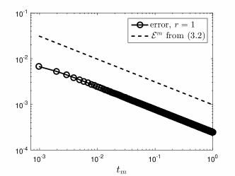
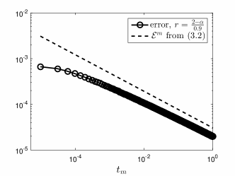
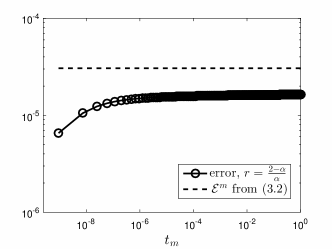
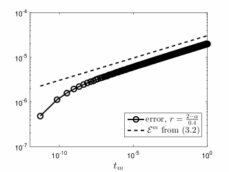
Fig. 1: L1 method applied to the initial-value test problem: pointwise errors for $\alpha=0.5$ and $M=1024$, cases $r=1$, $r=(2-\alpha)/0.9$, $r=(2-\alpha)/\alpha$ and $r=(2-\alpha)/0.4$.

Table 4: Alikhanov method applied to the initial-value test problem: errors at $t=1$ (odd rows) and computational rates $q$ in $M^{-q}$ (even rows) for $r=1$, $r=2$ and $r=(3-\alpha)/.95$

		$\;\;\;M=2^{6}$	$M=2^{8}$	$M=2^{10}$	$M=2^{12}$	$M=2^{14}$	$M=2^{16}$
$r=1$	$\alpha=0.3$	1.325e-3	3.306e-4	8.260e-5	2.065e-5	5.162e-6	1.290e-6
		1.002	1.000	1.000	1.000	1.000
	$\alpha=0.5$	1.530e-3	3.819e-4	9.543e-5	2.386e-5	5.964e-6	1.491e-6
		1.001	1.000	1.000	1.000	1.000
	$\alpha=0.7$	1.236e-3	3.087e-4	7.715e-5	1.929e-5	4.821e-6	1.205e-6
		1.001	1.000	1.000	1.000	1.000
$r=2$	$\alpha=0.3$	3.891e-5	2.446e-6	1.530e-7	9.560e-9	5.975e-10	3.734e-11
		1.996	1.999	2.000	2.000	2.000
	$\alpha=0.5$	6.079e-5	3.940e-6	2.502e-7	1.576e-8	9.885e-10	6.190e-11
		1.974	1.988	1.995	1.997	1.999
	$\alpha=0.7$	6.450e-5	4.436e-6	2.936e-7	1.902e-8	1.216e-09	7.720e-11
		1.931	1.959	1.974	1.984	1.989
$r=\frac{3-\alpha}{.95}$	$\alpha=0.3$	1.085e-5	3.241e-7	8.953e-9	2.363e-10	6.058e-12	1.509e-13
		2.532	2.589	2.622	2.643	2.664
	$\alpha=0.5$	2.710e-5	1.057e-6	3.839e-8	1.337e-9	4.529e-11	1.517e-12
		2.340	2.392	2.422	2.442	2.450
	$\alpha=0.7$	3.962e-5	2.017e-6	9.638e-8	4.431e-9	1.986e-10	8.791e-12
		2.148	2.194	2.221	2.240	2.249

Table 5: Alikhanov method applied to the initial-value test problem: maximum nodal errors (odd rows) and computational rates $q$ in $M^{-q}$ (even rows) for $r=1$, $r=2/\alpha$ and $r=(3-\alpha)/\alpha$

		$\;\;\;M=2^{6}$	$M=2^{8}$	$M=2^{10}$	$M=2^{12}$	$M=2^{14}$	$M=2^{16}$
$r=1$	$\alpha=0.3$	2.477e-2	1.634e-2	1.078e-2	7.115e-3	4.694e-3	3.097e-3
		0.300	0.300	0.300	0.300	0.300
	$\alpha=0.5$	1.164e-2	5.819e-3	2.909e-3	1.455e-3	7.273e-4	3.637e-4
		0.500	0.500	0.500	0.500	0.500
	$\alpha=0.7$	3.919e-3	1.485e-3	5.627e-4	2.132e-4	8.079e-5	3.061e-5
		0.700	0.700	0.700	0.700	0.700
$r=\frac{2}{\alpha}$	$\alpha=0.3$	5.865e-5	3.665e-6	2.291e-7	1.432e-8	8.949e-10	5.593e-11
		2.000	2.000	2.000	2.000	2.000
	$\alpha=0.5$	5.250e-5	3.281e-6	2.051e-7	1.282e-8	8.011e-10	5.007e-11
		2.000	2.000	2.000	2.000	2.000
	$\alpha=0.7$	4.232e-5	2.645e-6	1.653e-7	1.033e-8	6.458e-10	4.036e-11
		2.000	2.000	2.000	2.000	2.000
$r=\frac{3-\alpha}{\alpha}$	$\alpha=0.3$	5.505e-5	1.659e-6	4.472e-8	1.142e-9	2.833e-11	6.923e-13
		2.526	2.607	2.646	2.667	2.677
	$\alpha=0.5$	3.976e-5	1.379e-6	4.508e-8	1.439e-9	4.542e-11	1.425e-12
		2.425	2.467	2.485	2.493	2.497
	$\alpha=0.7$	3.425e-5	1.498e-6	6.307e-8	2.619e-9	1.083e-10	4.469e-12
		2.257	2.285	2.295	2.298	2.299

5.4 Alikhanov method: pointwise sharpness of the error estimate for the initial-value problem

Next, we turn to the Alikhanov method and, to demonstrate the sharpness of the error estimate (4.5) given by Theorem 18, consider the simplest initial-value fractional-derivative test problem (4.4) with the same simplest typical exact solution $u(t):=t^{\alpha}$. Table 4 shows the errors and the corresponding convergence rates at $t=1$, which agree with (4.5), in view of Remark 19. In particular, the latter implies that the errors are $\lesssim M^{-\min\{r,3-\alpha\}}$ for $r\neq 3-\alpha$. The maximum errors and corresponding convergence rates given in Table 5 clearly confirm the conclusions of Remark 20, which predicts from the pointwise bound (4.5) that the global errors are $\lesssim M^{-\min\{\alpha r,3-\alpha\}}$.

Note that, similarly to Fig. 1, we observed the pointwise behaviour of the errors consistent with (4.5); see also [11, Fig. 6.2] for similar graphs of pointwise errors of an L2-type method.

References

- [1] A. A. Alikhanov, A new difference scheme for the time fractional diffusion equation, J. Comput. Phys., 280 (2015), pp. 424–438.
- [2] H. Brunner, The numerical solution of weak singular Volterra integral equations by collocation on graded meshes, Math. Comp., 45 (1985), pp. 417–437.
- [3] H. Brunner, Collocation methods for Volterra integral and related functional differential equations, Cambridge University Press, Cambridge, UK, 2004.
- [4] H. Chen and M. Stynes, Error analysis of a second-order method on fitted meshes for a time-fractional diffusion problem, J. Sci. Comput., 79 (2019), pp. 624–647.
- [5] K. Diethelm, The analysis of fractional differential equations, Lecture Notes in Mathematics, Springer-Verlag, Berlin, 2010.
- [6] J. L. Gracia, E. O’Riordan and M. Stynes, Convergence in positive time for a finite difference method applied to a fractional convection-diffusion problem, Comput. Methods Appl. Math., 18 (2018), pp. 33–42
- [7] B. Jin, R. Lazarov and Z. Zhou, Two fully discrete schemes for fractional diffusion and diffusion-wave equations with nonsmooth data, SIAM J. Sci. Comput., 38 (2016), pp. A146–A170.
- [8] B. Jin, R. Lazarov and Z. Zhou, An analysis of the L1 scheme for the subdiffusion equation with nonsmooth data, IMA J. Numer. Anal., 36 (2016), 197–221.
- [9] B. Jin, R. Lazarov and Z. Zhou, Numerical methods for time-fractional evolution equations with nonsmooth data: a concise overview, Comput. Methods Appl. Mech. Engrg., 346 (2019), pp. 332–358.
- [10] N. Kopteva, Error analysis of the L1 method on graded and uniform meshes for a fractional-derivative problem in two and three dimensions, Math. Comp., 88 (2019), pp. 2135–2155.
- [11] N. Kopteva, Error analysis of an L2-type method on graded meshes for a fractional-order parabolic problem, Math. Comp. (2020), to appear; arXiv:1905.05070.
- [12] N. Kopteva, Error analysis for time-fractional semilinear parabolic equations using upper and lower solutions, arXiv:2001.04452, (2020).
- [13] H.-L. Liao, D. Li and J. Zhang, Sharp error estimate of the nonuniform L1 formula for linear reaction-subdiffusion equations, SIAM J. Numer. Anal., 56 (2018), pp. 1112–1133.
- [14] H.-L. Liao, W. McLean and J. Zhang, A second-order scheme with nonuniform time steps for a linear reaction-subdiffusion problem, arXiv:1803.09873v4, (2018).
- [15] H.-L. Liao, W. McLean and J. Zhang, A discrete Grönwall inequality with application to numerical schemes for fractional reaction-subdiffusion problems, SIAM J. Numer. Anal., 57 (2019), pp. 218–237.
- [16] W. McLean and K. Mustapha, A second-order accurate numerical method for a fractional wave equation, Numer. Math., 105 (2007), pp. 481–510.
- [17] K. Mustapha, B. Abdallah and K. M. Furati, A discontinuous Petrov-Galerkin method for time-fractional diffusion equations, SIAM J. Numer. Anal., 52 (2014), pp. 2512–2529.
- [18] K. Sakamoto and M. Yamamoto, Initial value/boundary value problems for fractional diffusion-wave equations and applications to some inverse problems, J. Math. Anal. Appl., 382 (2011), pp. 426–447.
- [19] M. Stynes, Too much regularity may force too much uniqueness, Fract. Calc. Appl. Anal., 19 (2016), pp. 1554–1562.
- [20] M. Stynes, E. O’Riordan and J. L. Gracia, Error analysis of a finite difference method on graded meshes for a time-fractional diffusion equation, SIAM J. Numer. Anal., 55 (2017), pp. 1057–1079.