Power-law Temperature Dependence of the Penetration Depth in a Topological Superconductor due to Surface States

Abstract

We study the temperature dependence of the magnetic penetration depth in a 3D topological superconductor (TSC), incorporating the paramagnetic current due to the surface states. A TSC is predicted to host a gapless 2D surface Majorana fluid. In addition to the bulk-dominated London response, we identify a $T^{3}$ power-law-in-temperature contribution from the surface, valid in the low-temperature limit. Our system is fully gapped in the bulk, and should be compared to bulk nodal superconductivity, which also exhibits power-law behavior. Power-law temperature dependence of the penetration depth can be one indicator of topological superconductivity.

A decade after the widespread infiltration of topology into quantum materials research, the search for electronically correlated topological phases beyond the fractional quantum Hall effect remains an urgent, but still largely unfulfilled quest. Topological superconductivity Qi_Zhang_Review ; Sato_Ando_Review is sought as a platform for Majorana fermion zero modes Jason_Review and topological quantum computation Q_computer1 . Majorana fermions could be detected by various means, including tunneling spectroscopy MF_STM1 ; MF_STM2 ; MF_STM3 ; MF_STM4 ; MF_STM5 , the Josephson effect 4pi_JE1 ; 4pi_JE2 ; MF_STM1 , as well as spin and optical responses spin_resp_TSC ; optical_resp_TSC .

Only a handful of materials have emerged as bulk topological superconductor (TSC) candidates. Topological superconductivity has long been suspected in Sr₂RuO₄, although a consensus on chiral $p$-wave order is yet to be reached Sato_Ando_Review ; Mackenzie-Maeno03 ; Kallin12 ; Kallin16 . Time-reversal invariant TSCs could serve as solid-state analogs of the topological superfluid phase in liquid helium (³He-$B$) Ludwig08 ; Roy08 ; Volovik09 ; Qi09 ; Sato09 ; Sato10 ; Machida16 . In the absence of a magnetic field, the predicted hallmark of such a bulk TSC is a gapless, two-dimensional (2D) Majorana fermion surface fluid. It has been argued that the odd-parity “$\hat{\bm{\mathrm{s}}}\cdot\bm{\mathrm{k}}$” pairing of ³He-$B$ VolovikBook ; BernevigHughesBook could naturally arise in doped Dirac semimetals or topological insulators CuBiSe_pairing ; CuBiSe_Anisopairing ; Wray10 ; here $\hat{\bm{\mathrm{s}}}$ and $\bm{\mathrm{k}}$ respectively denote the spin-operator and momentum vectors. Alternately, doped Weyl semimetals have been shown to be natural platforms for topological superconductivity Hosur14 .

There is now substantial experimental evidence for nematicity in the superconducting doped topological insulators (Cu,Nb)_xBi₂Se₃ Zheng16 ; Yonezawa17 ; Qiu17 ; Tao18 (see also Wen18 ), possibly indicative of odd-parity pairing. However, gapless Majorana fermions have not been conclusively detected Ando11 ; Chu13 ; Stroscio13 ; Tao18 . Recently, signatures consistent with topological superconductivity were also found in doped $\beta$-PdBi₂, but a conclusive detection remains elusive Kolapo18 . In Cu_xBi₂Se₃, only a small percentage of the exposed crystal surface was found to exhibit signatures of superconductivity in STM Tao18 , highlighting the possibility that in inhomogeneous TSCs, there is no guarantee that Majorana fermions will appear at the physical surface of the sample.

It is therefore natural to seek global probes of topological superconductivity. Meissner effect penetration depth measurements in Nb_xBi₂Se₃ Smylie16 ; Smylie17 and in the half-Heusler compounds YPtBi Paglione18 , YPdBi and TbPdBi Spinu18 exhibit power-law temperature suppression, which is interpreted as evidence for non-$s$-wave, bulk nodal superconductivity Tinkham . In the case of Nb_xBi₂Se₃, the results were interpreted as indicative of nodal odd-parity bulk pairing Smylie16 ; Smylie17 , while the YPtBi results were attributed to either an exotic nodal-line “septet” pairing scenario Paglione18 ; Brydon16 , or $d+id$ bulk Weyl superconductivity Brydon16 , smeared by disorder Roy19 .

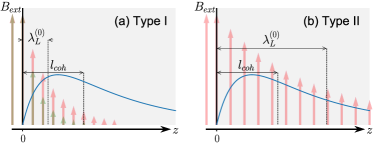
Figure 1: Schematic illustration for (a) type I and (b) type II topological superconductors (TSCs) in an external magnetic field. The gray and white regions represent respectively the TSC and the vacuum. The red (green) arrows indicate the magnetic field that decays into the superconductor with (without) the correction due to the surface states. The scale $\lambda_{L}^{{\scriptscriptstyle{(0)}}}$ is the London (bulk-dominated diamagnetic) penetration depth. The blue line is a sketch of the Majorana surface fluid density, characterized by the coherence length $l_{\mathsf{coh}}$.

In this Letter, we show that power-law temperature ($T$) dependence of the penetration depth $\lambda(T)$ can arise at arbitrarily low $T$ in a TSC with a fully gapped bulk, due to the paramagnetic response of the gapless Majorana surface fluid. This requires a nontrivial calculation employing a TSC model with a physical surface-vacuum boundary, and the result involves the convolution of the surface paramagnetic and bulk-dominated diamagnetic responses. It cannot be obtained from the surface Hamiltonian alone. Thus, the observation of non-exponential behavior in $\lambda(T)$ does not necessarily indicate bulk nodal pairing, and can be one diagnostic for screening possible TSCs. We also show that the magnetic field in a fully gapped TSC is sensitive to the spatial profile of the surface states. This can be used to differentiate gapless states from the surface versus those from the bulk. By contrast, STM is sensitive only to the sample surface density of states, while the finite energy resolution of ARPES might prevent the direct detection of Majorana fermions in a low-temperature superconductor. While power-law temperature dependence in the penetration depth can arise from multiple mechanisms Giannetta06 ; Cooper97 , it can serve as one possible indicator for bulk topological superconductivity. In general, one wants as many independent tests as possible in order to identify TSCs.

We consider “minimal” TSCs in class DIII with winding number $\nu=1$, possessing a single surface Majorana cone. We show that the leading correction to the London response due to the presence of Majorana surface states scales as $T^{3}$. The same temperature dependence is predicted to arise in the suppression of the mass flow of superfluid ³He-$B$ through a channel, due to surface currents Wu13 . We calculate explicitly the magnetic field profile inside the slab, which incorporates new features introduced by the surface states. For type I TSCs, the field penetrates much deeper than the London depth into the bulk, with the scale set by the coherence length. For type II TSCs the field is modulated in a shallow region near the surface, and then decays at deeper depths according to the London length, but with an enhanced field amplitude.

Model.—We consider a superconducting slab filling up the $z>0$ half-space, with an external magnetic field $\textbf{B}_{\mathsf{ext}}=B_{0}\,\hat{y}$ as shown in Fig. 1. We assume the field is weak enough such that $B_{0}<B_{c_{1}}$ where $B_{c_{1}}$ is the lower critical field of a type II superconductor. Under this assumption, the effect of vortex formation can be neglected and a linear response treatment is valid. The total current $\bm{\mathrm{J}}$ and the vector potential $\bm{\mathrm{A}}$ satisfy the static Maxwell’s equation

$$\bm{\nabla}^{2}\textbf{A}(z)=-\frac{4\pi}{c}\textbf{J}(z),$$ (1)

where $\textbf{A}(z)=A(z)\,\hat{x}$, $\bm{\mathrm{B}}(z)=\partial_{z}A(z)\,\hat{y}$, $\textbf{J}(z)=J(z)\,\hat{x}$, and

$$\textbf{J}(z)=\textbf{J}_{\mathsf{ext}}(z)-\frac{1}{c}\int_{0}^{\infty}dz^{\prime}\,\Pi(z,z^{\prime})\,\textbf{A}(z^{\prime}).$$ (2)

Here, $\textbf{J}_{\mathsf{ext}}(z)$ is a fictitious current generating the external magnetic field, and $\Pi(z,z^{\prime})$ is the current-current correlation function capturing the linear response of the TSC. The above equations can be expressed as

$$-2B_{0}= \,\left[q_{z}^{2}+\left(\lambda_{L}^{{\scriptscriptstyle{(0)}}}\right)^{-2}\right]\tilde{A}(q_{z})$$ (3)

$$\,+\frac{4\pi}{c^{2}}\int\frac{dQ_{z}}{2\pi}\,\tilde{\Pi}^{xx}_{1,R}(0,0,0;q_{z},-Q_{z})\,\tilde{A}(Q_{z}),$$

where $\lambda_{L}^{{\scriptscriptstyle{(0)}}}$ is the London penetration depth and

$$\tilde{\Pi}^{xx}_{1,R}(\Omega=0,q_{x}=0,q_{y}=0;q_{z},-Q_{z})$$ (4)

$$\;\;=-i\int dt\,dx\,dy\int_{0}^{\infty}dz_{1}dz_{2}\operatorname{e}^{-iq_{z}z_{1}+iQ_{z}z_{2}}$$

$$\qquad\qquad\qquad\times\left\langle\left[J_{1}^{x}(t,x,y,z_{1}),J_{1}^{x}(0,0,0,z_{2})\right]\right\rangle\theta(t)$$

is the retarded paramagnetic current-current correlation function. Here, $J_{1}^{x}(t,x,y,z)$ is the paramagnetic current flowing along the $x$ direction and $\theta(t)$ is the Heaviside step function. The first term on the right-hand-side of Eq. (3) represents the diamagnetic London response, while the second term is the paramagnetic response from both the bulk and surface states. The above framework is general and the magnetic field in the slab is determined once the current-current correlation function is specified. In what follows we consider a clean system. Weak nonmagnetic disorder is not expected to modify the low-temperature response of the surface response (it is strongly irrelevant Ghorashi19 ) or of the fully gapped bulk.

Although the low-temperature, $T^{3}$-dependence of the penetration depth derived below depends only on the low-energy dispersion of the 2D Majorana surface fluid, here we consider a microscopic model for both the bulk and surface modes of the TSC in order to completely specify the problem. Solid state models analogous to ³He provide a fertile playground to study topologically nontrivial superconductivity Sato_Ando_Review ; VolovikBook ; Volovik09 . “Solid-state ³He-$A$” would correspond to a Weyl superconductor, which has nodal Weyl points in the bulk that connect to a surface Majorana arc. In this work, we consider “solid-state ³He-$B$” VolovikBook ; BernevigHughesBook , with isotropic $p$-wave pairing of spin-1/2 electrons, represented by the following Bogoliubov-de Gennes Hamiltonian

$$H=\frac{1}{2}\int_{\textbf{k}}\chi^{\dagger}(\textbf{k})\,\hat{h}(\textbf{k})\,\chi(\textbf{k}),$$ (5)

where

$$\hat{h}(\textbf{k})=\tilde{\varepsilon}_{k}\,\hat{\sigma}^{3}+\Delta\,\hat{\textbf{s}}\cdot\textbf{k}\,\hat{\sigma}^{2},\qquad\tilde{\varepsilon}_{k}=\frac{k^{2}}{2m}-\mu,$$ (6)

and where $\int_{\textbf{k}}\equiv\int\frac{d^{3}\textbf{k}}{(2\pi)^{3}},$ $\hat{\textbf{s}}$ and $\bm{\hat{\sigma}}$ respectively denote Pauli matrices acting in the spin and particle-hole spaces, and $\chi(\textbf{k})\equiv\left[c(\textbf{k}),\hat{s}^{2}\left[c^{\dagger}(-\textbf{k})\right]^{\mathsf{T}}\right]$ is the four-component Balian-Werthammer spinor BW63 . The latter satisfies the reality (“Majorana”) condition $\chi^{\dagger}(\textbf{k})=i\chi^{\mathsf{T}}(-\textbf{k})\,\hat{M}_{\mathsf{P}},$ where $\hat{M}_{\mathsf{P}}=\hat{s}^{2}\hat{\sigma}^{2}$ defines particle-hole symmetry for $\hat{h}(\bm{\mathrm{k}})$. In Eq. (6), $\mu$ is the chemical potential and $\Delta$ is the superconducting order parameter amplitude. For $\mu>0$ the above Hamiltonian has winding number $\nu=1$. The retarded paramagnetic current-current correlation function due to the bulk is

$$\!\!\!\tilde{\Pi}_{1,R}^{xx}(\Omega=0,\textbf{q}=0)=-\frac{\beta}{6}\left(\frac{e}{m}\right)^{2}\int_{\textbf{k}}k^{2}\operatorname{sech}^{2}\left(\frac{\beta E_{k}}{2}\right)\!,\!\!\!$$ (7)

where $E_{k}=\sqrt{\tilde{\varepsilon}_{k}^{2}+\Delta^{2}k^{2}}$ is the eigenenergy of $\hat{h}(\textbf{k})$ and $\beta=T^{-1}$ is the inverse temperature. In the low-temperature limit, the bulk paramagnetic response is exponentially suppressed and the diamagnetic London response dominates. The London depth is given by $\lambda_{L}^{{\scriptscriptstyle{(0)}}}=\sqrt{mc^{2}/(4\pi e^{2}n)},$ where $n$ is the charge number density.

To consider the response from the surface, we replace $k_{z}\rightarrow-i\partial_{z}$ in $\hat{h}(\textbf{k})$ [Eq. (6)] and solve for the Majorana surface states $\psi_{\textbf{k}}^{\mathsf{s}}(z)$ with eigenenergies $\pm\Delta|\textbf{k}|$. Here and in what follows, $\textbf{k}=(k_{x},k_{y})$ specifies the momentum transverse to the interface. With hard wall boundary conditions at $z=0$, we obtain surface wave functions of the form SM

$$\psi_{\textbf{k}}^{\mathsf{s}}(z)=\frac{e^{-z/l_{\mathsf{coh}}}}{\sqrt{N_{\textbf{k}}^{\mathsf{s}}}}\,\sin\left(z\sqrt{\lambdabar_{F}^{-2}-l_{\mathsf{coh}}^{-2}-k^{2}}\right)\ket{\psi_{\textbf{k}}^{0}},$$ (8)

where $N_{k}^{\mathsf{s}}$ is a normalization constant and $\ket{\psi_{\textbf{k}}^{0}}$ is a spin-momentum-locked spinor in (spin)$\otimes$(particle-hole) space. The two length scales in Eq. (8) are the (reduced) Fermi wavelength $\lambdabar_{F}\equiv 1/\sqrt{2m\mu}$ and the coherence length $l_{\mathsf{coh}}\equiv 1/m\Delta$.

We can see how the magnetic field couples to the surface fluid by incorporating a vector potential $\bm{\mathrm{A}}$ into Eq. (5), and then projecting onto the low-energy surface states. The result is

$$H_{\mathsf{s}}=\int_{\textbf{r}}\left\{\frac{1}{2}\eta^{\dagger}(\textbf{r})\left[-i\Delta(\hat{s}\wedge\bm{\nabla})\right]\eta(\textbf{r})-\frac{1}{c}\textbf{A}\cdot\textbf{J}\right\},$$ (9)

where $\eta=\eta_{s}$ is the two-component surface Majorana fermion operator ($s\in\{\uparrow,\downarrow\}$), $\hat{s}\wedge\bm{\nabla}\equiv\hat{s}^{1}\partial_{y}-\hat{s}^{2}\partial_{x},$ and the surface paramagnetic current operator

$$\textbf{J}(\textbf{r})=\frac{e}{4m}\eta^{\dagger}(\textbf{r})i\bm{\overleftrightarrow{\nabla}}\eta(\textbf{r}).$$ (10)

Here $\textbf{r}=(x,y)$ and $\bm{\overleftrightarrow{\nabla}}\equiv\bm{\overrightarrow{\nabla}}-\bm{\overleftarrow{\nabla}}$. Eq. (9) assumes that the field $\bm{\mathrm{B}}(z)$ and the vector potential $\bm{\mathrm{A}}(z)$ (in London gauge) both reside in the $(x,y)$ plane. Zeeman coupling to a nonzero component $B_{z}$ would induce a Majorana mass, gapping out the surface fluid Qi_Zhang_Review , but this is prevented by bulk Meissner screening. On the other hand, a very strong in-plane field $A_{x,y}$ could “overtilt” the surface Majorana cone, creating a surface Fermi pocket. The latter should be included in the diamagnetic current Guinea19 , but we exclude this situation here by restricting to linear response.

In the low-temperature limit, the paramagnetic current-current correlation function due to the surface state fluid evaluates to SM

$$\tilde{\Pi}_{1,R,\mathsf{s},\mathsf{s}}^{xx}(0,0,0;q_{z},-Q_{z})$$ (11)

$$\qquad\simeq-\mathcal{C}\,\left(\frac{e}{m}\right)^{2}\frac{(k_{B}T)^{3}}{\Delta^{4}}\,\Theta(0,q_{z})\,\Theta(0,-Q_{z}),$$

$\mathcal{C}\equiv\left[3^{2}\zeta(3)/(2^{3}\pi)\right]$, $\zeta(z)$ is the Riemann Zeta function, and where

$$\Theta(k,q_{z})\equiv\int_{0}^{\infty}dz\,\operatorname{e}^{-iq_{z}z}\,\psi_{\textbf{k}}^{\mathsf{s}\dagger}(z)\,\psi_{\textbf{k}}^{\mathsf{s}}(z)$$ (12)

is the Fourier transformed probability density of the surface states along the $z$-direction. Unlike the paramagnetic response from the bulk, the one from the surface [Eq. (11)] has a non-trivial $T^{3}$ power-law dependence at low temperature. Two factors of temperature arise from the form of the paramagnetic current operator (a derivative) in Eq. (10), while the third stems from the surface density of states of the Majorana fluid. One should also consider the surface-bulk cross terms when evaluating the paramagnetic current-current correlator appearing in Eq. (3). However, these cross terms exhibit higher-power temperature-dependence at low $T$, and are thus subleading SM . We neglect these surface-bulk contributions in the following.

Results.—Taking only the diamagnetic and surface paramagnetic responses into account, which is valid at low temperature as discussed above, we can formally invert the integral equation Eq. (3) and solve for the vector potential (and hence the magnetic field) profile inside the slab. To leading order in temperature, the final result is SM

$$B_{y}(z)=B_{0}\left\{\operatorname{e}^{-z/\lambda_{L}^{{\scriptscriptstyle{(0)}}}}-\varrho(T)\bigg{[}\partial_{z}G(z)\bigg{]}G(0)\right\},$$ (13)

where

$$\varrho(T)\equiv\left[2^{4}3^{3}\zeta(3)\pi\right]\left(\lambda_{L}^{{\scriptscriptstyle{(0)}}}\right)^{6}\,l_{\mathsf{coh}}^{-1}\,\lambdabar_{F}^{-4}\,t^{3}$$ (14)

is a temperature-dependent length, with $t\equiv k_{B}T/\Delta k_{F}$ being the dimensionless temperature. Here, $\Delta k_{F}$ is the energy gap of the $p$-wave TSC. In Eq. (13), the function $G(z)$ is a temperature-independent, real-valued function encoding the convolution of the bulk and surface responses. It is a dimensionless function only of $z$ and of the three lengths $\{\lambdabar_{F},\lambda_{L}^{{\scriptscriptstyle{(0)}}},l_{\mathsf{coh}}\}$. $G(z)$ emerges when we invert the integral equation and Fourier transform the quantities back to real space SM .

The first term in Eq. (13) describes the Meissner screening due to the diamagnetic London response, while the second term is the correction due to the Majorana surface fluid. The correction term depends on the length $\varrho(T)$ that encodes the $T^{3}$ dependence, while its spatial dependence is captured by $G(z)$. The function $G(z)$ decays exponentially for large $z$; its spatial extent is governed by the maximum of $\{\lambda_{L}^{{\scriptscriptstyle{(0)}}},l_{\mathsf{coh}}/2\}$, assuming that $\lambdabar_{F}$ is the shortest scale. This leads to different qualitative type I and II behaviors. Nevertheless, to characterize the overall spatial extent of the magnetic field, we can define the effective penetration depth of the system via Tinkham

$$\lambda(T)\equiv\frac{1}{B_{0}}\int_{0}^{\infty}dz\,B_{y}(z)=\lambda_{L}^{{\scriptscriptstyle{(0)}}}+\varrho(T)\left[G(0)\right]^{2}.$$ (15)

The second term in Eq. (15) is the change of the penetration depth due to the surface states. This term is always positive, meaning that the magnetic field can penetrate deeper into the slab for any $T>0$, due to the surface Majorana fluid. It is instructive to roughly estimate the order of magnitude for such correction. For Cu_xBi₂Se₃, which is in the extreme type II regime, we substitute typical experimental data $l_{\mathsf{coh}}\sim 10$ nm, $\lambdabar_{F}\sim 1$ nm, and $\lambda_{L}^{{\scriptscriptstyle{(0)}}}\sim 1$ $\mu$m Ando12 ; Tao18 to obtain $\delta\lambda(T)\sim 0.1\lambda_{L}^{{\scriptscriptstyle{(0)}}}t^{3}$.

The two physical quantities $B_{y}(z)$ and $\lambda(T)$ we focus on inherit the $T^{3}$ dependence from the surface current-current correlation function [Eq. (11)]. Similar power-law-dependence is observed in bulk nodal superconductors. In contrast to those systems, the model we considered is fully gapped in the bulk, and thus the Majorana surface states are responsible for the gapless excitations.

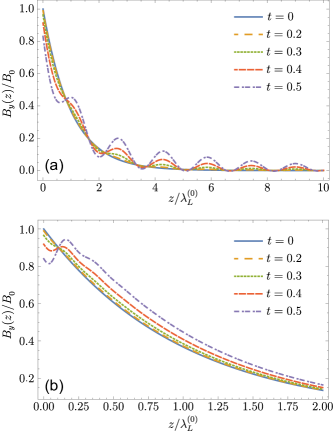
Figure 2: Plot of the magnetic field profile inside the topological superconductor (TSC) at different temperatures in the (a) type-I case with $\lambda_{L}^{{\scriptscriptstyle{(0)}}}=1$, $l_{\mathsf{coh}}=10$, and $\lambdabar_{F}=0.5$, and (b) type-II case with $\lambda_{L}^{{\scriptscriptstyle{(0)}}}=30$, $l_{\mathsf{coh}}=8$, and $\lambdabar_{F}=2$. Here $\lambdabar_{F}=1/\sqrt{2m\mu}$ is the reduced Fermi wavelength, $l_{\mathsf{coh}}=1/m\Delta$ is the coherence length, and $\lambda_{L}^{{\scriptscriptstyle{(0)}}}$ is the London depth. The blue curves (at $t=0$) represent the diamagnetic London response. The dimensionless temperature $t\equiv k_{B}T/\Delta k_{F}$, where $\Delta k_{F}$ is the $p$-wave TSC energy gap. As temperature increases, the response from the surface becomes more pronounced. For type I (a), the correction from the surface exhibits Friedel oscillations and penetrates much deeper than the London depth. For type II (b), the strongest modulation due to the surface fluid appears close to the surface.

Although the exact expression for $G(z)$ is complicated SM , it takes relatively simple forms in the strong type-I and type-II limits. For a type-I TSC ($l_{\mathsf{coh}}\gg\lambda_{L}^{{\scriptscriptstyle{(0)}}}$),

$$\!\!\!\!\!\begin{aligned} G_{\mathrm{I}}(z)\simeq&\,\frac{\lambdabar_{F}^{2}}{2\left(\lambda_{L}^{{\scriptscriptstyle{(0)}}}\right)^{2}\left[4\left(\lambda_{L}^{{\scriptscriptstyle{(0)}}}\right)^{2}+\lambdabar_{F}^{2}\right]}\bigg{\{}-\left(\lambda_{L}^{{\scriptscriptstyle{(0)}}}\right)^{2}e^{-z/\lambda_{L}^{{\scriptscriptstyle{(0)}}}}\\ &\,+\left[2\left(\lambda_{L}^{{\scriptscriptstyle{(0)}}}\right)^{2}+\lambdabar_{F}^{2}\sin^{2}\left(\frac{z}{\lambdabar_{F}}\right)\right]e^{-2z/l_{\mathsf{coh}}}\bigg{\}}.\end{aligned}\!\!\!\!\!$$ (16)

Since the coherence length sets the depth of the surface fluid [Eq. (8)], the latter allows a much deeper penetration of the field in the type-I limit than the bulk London depth. The slower decay is modulated by a Friedel oscillation. Representative field profiles are shown in Fig. 2(a).

For a type-II TSC ($l_{\mathsf{coh}}\ll\lambda_{L}^{{\scriptscriptstyle{(0)}}}$),

$$G_{\mathrm{II}}(z)\simeq\frac{\lambdabar_{F}^{2}l_{\mathsf{coh}}}{16\left(\lambda_{L}^{{\scriptscriptstyle{(0)}}}\right)^{4}}\left[\lambda_{L}^{{\scriptscriptstyle{(0)}}}\,e^{-z/\lambda_{L}^{{\scriptscriptstyle{(0)}}}}-l_{\mathsf{coh}}\,e^{-2z/l_{\mathsf{coh}}}\right].$$ (17)

In this case the Friedel oscillating terms are subleading, and can be neglected. Note that the first term in Eq. (17) dominates the second. In this case the spatial field penetration is governed by the London depth, but the correction in Eqs. (13) and (17) effectively enhances the field amplitude. Representative field profiles are indicated in Fig. 2(b).

Conclusion.—Our calculations suggest an alternative way to search for Majorana surface states in TSCs by measuring the change in the penetration depth $\delta\lambda(T)$. ARPES is often employed as the key tool to detect smoking gun signatures of topology in quantum materials. Unfortunately, TSC candidates typically have a small gap, making surface states difficult for ARPES to resolve Wray10 . A necessary, but not sufficient condition for the existence of a gapless Majorana surface fluid can be the signature power-law dependence $\delta\lambda(T)\sim T^{3}$. This can be probed by means of tunnel-diode oscillator techniques Smylie16 ; Smylie17 ; Paglione18 ; Spinu18 . While $\delta\lambda(T)$ is exponentially suppressed in conventional, topologically trivial superconductors, a power-law $\delta\lambda(T)\sim T^{\alpha}$ is also expected in superconductors with nodal bulk excitations, where $\alpha$ depends on whether the nodes are points or lines Tinkham ; Sigrist_Review . For example, a power-law with $\alpha=1$ has been observed in high-$T_{c}$ $d$-wave superconductors Giannetta06 .

One way to distinguish the origin of a penetration-depth power law (Majorana surface states versus bulk nodes) is via a specific-heat measurement versus temperature. The specific heat due to the 2D surface of a fully gapped 3D TSC is negligible. In addition to $\delta\lambda(T)\sim T^{\alpha}$, a TSC with a fully gapped bulk (nodal superconductor) should therefore demonstrate exponential suppression (power-law dependence) in specific heat Sigrist_Review .

The superconducting doped topological insulators (Cu,Nb)_xBi₂Se₃ Ando12 ; Smylie16 ; Smylie17 and the half-Heusler compound YPtBi Paglione18 ; Bay12 are all strongly type II. Power-law dependence of $\lambda(T)$ was observed in Nb_xBi₂Se₃ Smylie16 ; Smylie17 , YPtBi Paglione18 , and in YPdBi and TbPdBi Spinu18 . It would be interesting to assess whether any of these could be attributed to the presence of Majorana surface states. In particular, it is worthwhile to note that while specific-heat measurements suggest a fully gapped bulk in Cu_xBi₂Se₃ and Ni_xBi₂Se₃Yonezawa17 ; Qiu17 , penetration depth data for Ni_xBi₂Se₃ shows a power-law dependence Smylie16 ; Smylie17 . In the case of half-Heusler compounds such as YPtBi, it has been suggested that optical-phonon-mediated pairing could favor a fully gapped TSC state with winding number $\nu=3$ Savary17 , and this should induce novel, cubic-dispersing Majorana surface fermions Fang15 ; Roy19 . In this case, we would expect a very slow $\delta\lambda(T)\sim T^{1/3}$ dependence for a clean, cubically-dispersing Majorana surface fluid. However, the results due to surface states with $\nu\geq 3$ might be strongly modified by quenched disorder Roy19 ; Foster14 .

In this Letter, calculations were performed for a clean system. On one hand, low-energy Majorana surface states with winding number $\nu=1$ are not affected by non-magnetic impurities Foster14 ; Ghorashi19 ; weak nonmagnetic disorder should therefore not alter the cubic power law $\delta\lambda(T)\sim T^{3}$ predicted here as $T\rightarrow 0$. The power can possibly be modified by strong (resonant) impurity scattering Giannetta06 . On the other hand, magnetic impurities can strongly perturb the surface states, and even gap them out. Moreover, magnetic impurities may independently induce power-law dependence in $\delta\lambda(T)$, by altering the magnetic permeability Giannetta06 ; Cooper97 .

We thank Andriy Nevidomskyy for useful discussions. T.C.W. and M.S.F. acknowledge support by the Welch Foundation Grant No. C-1809, by NSF CAREER Grant No. DMR-1552327, and by the U.S. Army Research Office Grant No. W911NF-17-1-0259. M.S.F. thanks the Aspen Center for Physics, which is supported by the NSF Grant No. PHY-1607611, for its hospitality while part of this work was performed. P.H. and H.K.P. were supported by the Department of Physics, College of Natural Sciences and Mathematics at the University of Houston. H.K.P acknowledges support from IRCC, IIT Bombay (RD/0518-IRCCSH0-029).

I I. Majorana surface states

We solve for the surface states by converting $k_{z}\rightarrow-i\partial_{z}$ in Eq. (6),

$$\hat{h}(\textbf{k},-i\partial_{z})\,\psi_{\varepsilon}(z)=\varepsilon\,\psi_{\varepsilon}(z),$$ (S1)

where $\bm{\mathrm{k}}=(k_{x},k_{y})$ specifies the momentum transverse to the vacuum-TSC interface at $z=0$ (Fig. 1). For this model with a hard wall boundary condition at $z=0$, the surface Majorana fluid has an exactly linear dispersion relation $\varepsilon=\Delta k$, corresponding to the surface wave function [Eq. (8)]

$$\psi_{\textbf{k}}^{\mathsf{s}}(z)=\frac{1}{\sqrt{N_{\textbf{k}}^{\mathsf{s}}}}\,e^{-z/l_{\mathsf{coh}}}\,\sin\left(z\sqrt{\lambdabar_{F}^{-2}-l_{\mathsf{coh}}^{-2}-k^{2}}\right)\begin{bmatrix}1\\ -ie^{i\phi_{\textbf{k}}}\\ 1\\ ie^{i\phi_{\textbf{k}}}\end{bmatrix},$$ (S2)

where $e^{i\phi_{\textbf{k}}}\equiv(k_{x}+ik_{y})/k$ and the normalization constant

$$N_{\bm{\mathrm{k}}}^{\mathsf{s}}=l_{\mathsf{coh}}\frac{\left(\lambdabar_{F}^{-2}-l_{\mathsf{coh}}^{-2}-k^{2}\right)}{\left(\lambdabar_{F}^{-2}-k^{2}\right)}.$$ (S3)

The four-component spinor in Eq. (S2) is expressed in the [spin ($s$)]$\otimes$[particle-hole ($\sigma$)] basis such that $\hat{s}^{3}\rightarrow\operatorname{diag}(1,-1,1,-1)$ and $\hat{\sigma}^{3}\rightarrow\operatorname{diag}(1,1,-1,-1)$.

The Bogoliubov-de Gennes Hamiltonian $\hat{h}(\bm{\mathrm{k}})$ in Eq. (6) has the following particle-hole (P), time-reversal (T), and chiral (S) symmetries:

$$-\hat{M}_{\mathsf{P}}^{-1}\,\hat{h}^{\mathsf{T}}(-\textbf{k})\,\hat{M}_{\mathsf{P}} = \hat{h}(\textbf{k}),\qquad\hat{M}_{\mathsf{P}}=\hat{s}^{2}\hat{\sigma}^{2}=\hat{M}_{\mathsf{P}}^{\mathsf{T}},$$ (S4)

$$\hat{M}_{\mathsf{T}}^{-1}\,\hat{h}^{*}(-\textbf{k})\,\hat{M}_{\mathsf{T}} = \hat{h}(\textbf{k}),\qquad\hat{M}_{\mathsf{T}}=i\hat{s}^{2}\hat{\sigma}^{3}=-\hat{M}_{\mathsf{T}}^{\mathsf{T}},$$ (S5)

$$-\hat{M}_{\mathsf{S}}\,\hat{h}(\textbf{k})\,\hat{M}_{\mathsf{S}} = \hat{h}(\textbf{k}),\qquad\hat{M}_{\mathsf{S}}=\hat{\sigma}^{1},$$ (S6)

where $\hat{A}^{\mathsf{T}}$ is the matrix transpose of $\hat{A}$. The chiral symmetry is a product of time-reversal and particle-hole; since the latter is an automatic consequence of fermion antisymmetry, chiral is equivalent to time-reversal.

The negative-energy surface eigenstate with momentum $\bm{\mathrm{k}}$ is the chiral transform of Eq. (S2), $\hat{\sigma}^{1}\,\psi_{\textbf{k}}^{\mathsf{s}}(z)$. Positive- and negative-energy surface states are bi-locally orthogonal (due to the spin-momentum–locked spinors),

$$\psi_{\textbf{k}}^{\mathsf{s}\dagger}(z_{1})\,\hat{\sigma}^{1}\,\psi_{\textbf{k}}^{\mathsf{s}}(z_{2})=\psi_{\textbf{k}}^{\mathsf{s}\dagger}(z_{1})\,\hat{s}^{3}\,\psi_{\textbf{k}}^{\mathsf{s}}(z_{2})=0.$$ (S7)

II II. Paramagnetic Current-Current Correlation Function

II.1 A. Correlation function from the bulk alone

The imaginary time action corresponding to Eq. (5) is

$$S = \frac{T}{2}\sum_{\omega_{n}}\int d^{3}\bm{\mathrm{r}}\,\chi^{\mathsf{T}}(-\omega_{n},\textbf{r})\,i\hat{M}_{\mathsf{P}}\left(-i\omega_{n}+\hat{h}\right)\chi(\omega_{n},\textbf{r}),$$ (S1)

where $\omega_{n}$ denotes a fermionic Matsubara frequency. The imaginary time paramagnetic current-current correlation function is

$$\Pi_{1}^{xx}(\tau,\textbf{r},\textbf{r}^{\prime})= \,\left\langle J_{1}^{x}(\tau,\textbf{r})\,J_{1}^{x}(0,\textbf{r}^{\prime})\right\rangle$$ (S2)

$$= \,-\frac{1}{2}\left(\frac{e}{m}\right)^{2}T^{2}\sum_{\omega_{1},\omega_{2}}\int_{\textbf{k}_{1},\textbf{k}_{2}}e^{-i(\omega_{1}-\omega_{2})\tau+i(\textbf{k}_{1}-\textbf{k}_{2})\cdot(\textbf{r}-\textbf{r}^{\prime})}\,(k_{1}^{x})(k_{2}^{x})\,\mathsf{Tr}\left[\hat{G}(i\omega_{1},\textbf{k}_{1})\,\hat{G}(i\omega_{2},\textbf{k}_{2})\right],$$

where we have made use of the translational invariance in the bulk. Using the Green’s function $\hat{G}(i\omega,\textbf{k})=\left[-i\omega+\hat{h}(\textbf{k})\right]^{-1},$ the Fourier transformed correlation function is

$$\tilde{\Pi}^{xx}_{1}(i\Omega_{n}=0,\textbf{q}=0)= \,-\frac{2}{3}\left(\frac{e}{m}\right)^{2}T\sum_{\omega}\int_{\textbf{k}}k^{2}\,\frac{E_{k}^{2}-\omega^{2}}{(\omega^{2}+E_{k}^{2})^{2}}$$ (S3)

$$= \,\frac{\beta}{6}\left(\frac{e}{m}\right)^{2}\int_{\textbf{k}}k^{2}\operatorname{sech}^{2}\left(\frac{\beta E_{k}}{2}\right),$$

where $E_{k}=\sqrt{\tilde{\varepsilon}_{k}^{2}+\Delta^{2}k^{2}}$. The retarded version is given by Eq. (7) in the main text.

II.2 B. Correlation functions for the semi-infinite slab

To consider the effect of the surface, we must retain the $(z,z^{\prime})$-dependence of the Green’s function. Eqs. (S2) and (S3) are replaced by

$$\Pi_{1}^{xx}(\tau,\textbf{r}-\textbf{r}^{\prime},z,z^{\prime})=-\frac{1}{2}\left(\frac{e}{m}\right)^{2}T^{2}\sum_{\omega_{1},\omega_{2}}\int_{\textbf{k}_{1},\textbf{k}_{2}}e^{-i(\omega_{1}-\omega_{2})\tau+i(\textbf{k}_{1}-\textbf{k}_{2})\cdot(\textbf{r}-\textbf{r}^{\prime})}(k_{1}^{x})(k_{2}^{x})\,\mathsf{Tr}\left[\hat{G}(i\omega_{1},\textbf{k}_{1};z,z^{\prime})\,\hat{G}(i\omega_{2},\textbf{k}_{2};z^{\prime},z)\right]\!,$$ (S4)

where $\textbf{r}=(x,y)$ and $\textbf{k}=(k_{x},k_{y})$ are 2D vectors parallel to the interface. Then

$$\tilde{\Pi}_{1}^{xx}(i\Omega_{n}=0,\textbf{q}=0;z,z^{\prime})=-\frac{1}{2}\left(\frac{e}{m}\right)^{2}T\sum_{\omega}\int_{\textbf{k}}(k^{x})^{2}\,\mathsf{Tr}\left[\hat{G}(i\omega_{1},\textbf{k};z,z^{\prime})\,\hat{G}(i\omega_{2},\textbf{k};z^{\prime},z)\right].$$ (S5)

We assume a generic eigenstate decomposition for $\hat{G}$,

$$\hat{G}(i\omega,\textbf{k};z,z^{\prime})=\sum_{\varepsilon}\frac{\psi_{\varepsilon,\textbf{k}}(z)\,\psi^{\dagger}_{\varepsilon,\textbf{k}}(z^{\prime})}{-i\omega+\varepsilon},$$ (S6)

where the sum runs over all positive- and negative-energy bulk and surface states of $\hat{h}$ in Eq. (S1), so that

$$\tilde{\Pi}_{1}^{xx}(i\Omega_{n}=0,\textbf{q}=0;z,z^{\prime})=\frac{1}{2}\left(\frac{e}{m}\right)^{2}\int_{\textbf{k}}(k^{x})^{2}\sum_{\varepsilon_{1},\varepsilon_{2}}\left[\psi_{\varepsilon_{2},\textbf{k}}^{\dagger}(z)\,\psi_{\varepsilon_{1},\textbf{k}}(z)\,\psi_{\varepsilon_{1},\textbf{k}}^{\dagger}(z^{\prime})\,\psi_{\varepsilon_{2},\textbf{k}}(z^{\prime})\right]F(\varepsilon_{1},\varepsilon_{2}),$$ (S7)

where

$$F(\varepsilon_{1},\varepsilon_{2})\equiv \,-T\sum_{\omega}\frac{1}{(-i\omega+\varepsilon_{1})(-i\omega+\varepsilon_{2})}=\left\{\begin{aligned} &\,\displaystyle{\frac{\tanh\left(\frac{\beta\varepsilon_{1}}{2}\right)-\tanh\left(\frac{\beta\varepsilon_{2}}{2}\right)}{2(\varepsilon_{1}-\varepsilon_{2})},}\qquad&\varepsilon_{1}\neq\varepsilon_{2},\\ &\,\frac{\beta}{4}\operatorname{sech}^{2}\left(\frac{\beta\varepsilon_{1}}{2}\right),&\varepsilon_{1}=\varepsilon_{2}.\end{aligned}\right.$$ (S8)

For a system that is isotropic (rotationally invariant) in the $(x,y)$ plane parallel to the interface, the double-Fourier transform of the retarded version is

$$\tilde{\Pi}_{1,R}^{xx}(0,0,0;q_{z},-Q_{z})=-\frac{1}{4}\left(\frac{e}{m}\right)^{2}\int_{\textbf{k}}k^{2}\sum_{\varepsilon_{1},\varepsilon_{2}}F(\varepsilon_{1},\varepsilon_{2}) \,\left[\int_{0}^{\infty}dz\,e^{-iq_{z}z}\,\psi_{\varepsilon_{2},\textbf{k}}^{\dagger}(z)\,\psi_{\varepsilon_{1},\textbf{k}}(z)\right]$$

$$\times \,\left[\int_{0}^{\infty}dz^{\prime}\,e^{iQ_{z}z^{\prime}}\,\psi_{\varepsilon_{1},\textbf{k}}^{\dagger}(z^{\prime})\,\psi_{\varepsilon_{2},\textbf{k}}(z^{\prime})\right].$$ (S9)

II.2.1 1. Surface-surface response

The surface eigenstates $\psi_{\bm{\mathrm{k}}}^{\mathsf{s}}(z)$ and $\hat{\sigma}^{1}\,\psi_{\bm{\mathrm{k}}}^{\mathsf{s}}(z)$ [Eqs. (8) and (S2)] respectively have eigenenergies $\pm\Delta|\bm{\mathrm{k}}|$. The surface-surface contribution to Eq. (II.2) is

$$\tilde{\Pi}_{1,R;\mathsf{s},\mathsf{s}}^{xx}= \,-\frac{1}{2}\left(\frac{e}{m}\right)^{2}\int_{\textbf{k}}\frac{\beta k^{2}}{4}\operatorname{sech}^{2}\left(\frac{\beta\Delta k}{2}\right)\left[\int_{0}^{\infty}dz\,e^{-iq_{z}z}\psi_{\textbf{k}}^{\mathsf{s}\dagger}(z)\,\psi_{\textbf{k}}^{\mathsf{s}}(z)\right]\left[\int_{0}^{\infty}dz^{\prime}\,e^{iQ_{z}z^{\prime}}\,\psi_{\textbf{k}}^{\mathsf{s}\dagger}(z^{\prime})\,\psi_{\textbf{k}}^{\mathsf{s}}(z^{\prime})\right]$$ (S10)

$$= \,-\frac{\beta}{2^{4}\pi}\left(\frac{e}{m}\right)^{2}\int_{0}^{\lambdabar_{F}^{-1}}dk\,k^{3}\operatorname{sech}^{2}\left(\frac{\beta\Delta k}{2}\right)\,\Theta(k,q_{z})\,\Theta(k,-Q_{z}),$$

where we have used Eq. (S7), and where [Eq. (12)]

$$\Theta(k,q_{z})\equiv\int_{0}^{\infty}dz\,e^{-iq_{z}z}\,\psi_{\textbf{k}}^{\mathsf{s}\dagger}(z)\,\psi_{\textbf{k}}^{\mathsf{s}}(z)=\frac{8il_{\mathsf{coh}}^{-1}\left(k^{2}-\lambdabar_{F}^{-2}\right)}{\left[2il_{\mathsf{coh}}^{-1}-q_{z}\right]\left[4\left(k^{2}-\lambdabar_{F}^{-2}\right)-4il_{\mathsf{coh}}^{-1}q_{z}+q_{z}^{2}\right]}.$$ (S11)

The ultraviolet momentum cutoff $\lambdabar_{F}^{-1}=k_{F}$ in Eq. (S10) is where the surface Majorana band merges with the bulk quasiparticle continuum. For low temperatures $\beta\rightarrow\infty$, we can extend the upper limit of the $k$ integration to infinity, and drop the dependence of $\Theta(k,q)$ on $k$. To leading order in temperature, one obtains Eq. (11) in the main text.

II.2.2 2. Surface-bulk cross terms

The surface-bulk cross term contributions to Eq. (II.2) take the form

$$\tilde{\Pi}_{1,R,\mathsf{s},\mathsf{b}}^{xx}(0,0,0;q_{z},-Q_{z})=-\left(\frac{e}{m}\right)^{2}\int_{0}^{\lambdabar_{F}^{-1}}dk\,k^{3}\sum_{\mathsf{s},\mathsf{b}}\alpha_{\mathsf{s},\mathsf{b}}(\bm{\mathrm{k}};q_{z},-Q_{z})\,F\left[E_{\mathsf{s}}(\bm{\mathrm{k}}),E_{\mathsf{b}}(\bm{\mathrm{k}})\right],$$ (S12)

where $\alpha_{\mathsf{s},\mathsf{b}}(\bm{\mathrm{k}};q_{z},-Q_{z})$ is a temperature-independent coefficient encoding the $(q_{z},-Q_{z})$-transformed overlaps between the surface bound Majorana and bulk standing wave quasiparticle states. The summation runs over all surface and bulk eigenstates with eigenenergies $E_{\mathsf{s}}(\bm{\mathrm{k}})$ and $E_{\mathsf{b}}(\bm{\mathrm{k}})$, respectively. At low temperatures, the expression is dominated by small energies, but the mismatch between the gapless surface [$\lim_{k\rightarrow 0}|E_{\mathsf{s}}(\bm{\mathrm{k}})|=\Delta k\rightarrow 0$] and the gapped bulk [$\min|E_{\mathsf{b}}(\bm{\mathrm{k}})|=\Delta k_{F}$] means that the leading temperature dependence of this term is

$$\tilde{\Pi}_{1,R,\mathsf{s},\mathsf{b}}^{xx}(0,0,0;q_{z},-Q_{z})\sim T^{4},$$ (S13)

which is higher order than the contribution of the surface-surface term.

III III. Low-temperature field penetration

III.1 A. Solution to the integral equation

The kernel in Eq. (11) can be identified as the matrix elements of an outer product

$$\tilde{\Pi}_{1,R;\mathsf{s},\mathsf{s}}^{xx}=-\Upsilon\,\braket{q_{z}}{R}\braket{R}{Q_{z}},\qquad\Upsilon\equiv\left[\frac{2^{3}3^{2}\zeta(3)}{\pi}\right]\left(\frac{2m\mu e}{\Delta}\right)^{2}(k_{B}T)^{3}.$$ (S1)

Here we assume the norm and resolution of the identity,

$$\braket{q_{z}}{Q_{z}}=2\pi\delta(q_{z}-Q_{z}),\qquad\qquad\hat{1}=\int_{-\infty}^{\infty}\frac{dq_{z}}{2\pi}\ket{q_{z}}\bra{q_{z}}.$$ (S2)

The Meissner response in Eq. (3) can then be written as

$$-2B_{0}\int_{Q_{z}}\braket{q_{z}}{Q_{z}}= \,\left[q_{z}^{2}+\left(\lambda_{L}^{{\scriptscriptstyle{(0)}}}\right)^{-2}\right]\tilde{A}(q_{z})-\frac{4\pi\Upsilon}{c^{2}}\int_{Q_{z}}\braket{q_{z}}{R}\braket{R}{Q_{z}}\tilde{A}(Q_{z})$$ (S3)

$$= \,\bra{q_{z}}\left[\hat{M}(\hat{q}_{z})-\frac{4\pi\Upsilon}{c^{2}}\ket{R}\bra{R}\right]\ket{\tilde{A}},\qquad\hat{M}(\hat{q}_{z})\equiv\left[\hat{q}_{z}^{2}+\left(\lambda_{L}^{{\scriptscriptstyle{(0)}}}\right)^{-2}\right].$$

Formally, we can invert the operator to obtain

$$\tilde{A}(q_{z})= \,-2B_{0}\bra{q_{z}}\int_{Q_{z}}\hat{M}^{-1}(\hat{q}_{z})\left[\hat{1}-\frac{4\pi\Upsilon}{c^{2}}\ket{R}\bra{R}\hat{M}^{-1}(\hat{q}_{z})\right]^{-1}\ket{Q_{z}}$$ (S4)

$$= \,-2B_{0}\left\{M^{-1}(q_{z})+\left(\frac{4\pi\Upsilon\Xi}{c^{2}}\right)M^{-1}(q_{z})\,R(q_{z})\int_{Q_{z}}M^{-1}(Q_{z})\,R^{*}(Q_{z})\right\},$$

where

$$\Xi(T)\equiv\left\{1-\left(\frac{4\pi\Upsilon}{c^{2}}\right)\left[\bra{R}\hat{M}^{-1}(\hat{q}_{z})\ket{R}\right]\right\}^{-1}$$ (S5)

is a temperature-dependent constant that goes to $1+\bm{\mathit{O}}\left(T^{3}\right)$ as $k_{B}T\rightarrow 0$. Using $l_{\mathsf{coh}}=(m\Delta)^{-1}$, $\lambdabar_{F}=1/\sqrt{2m\mu}$, $\lambda_{L}^{{\scriptscriptstyle{(0)}}}=\sqrt{mc^{2}/(4\pi e^{2}n)}$, $n=k_{F}^{3}/3\pi^{2}$, and defining physical BCS gap as $\Delta_{BCS}=k_{F}\Delta$, we define

$$\varrho(T)\equiv\frac{8\pi\Upsilon}{c^{2}}\left(\lambda_{L}^{{\scriptscriptstyle{(0)}}}\right)^{8}=\bigg{[}2^{4}3^{3}\zeta(3)\pi\Xi(T)\bigg{]}\frac{\left(\lambda_{L}^{{\scriptscriptstyle{(0)}}}\right)^{6}}{l_{\mathsf{coh}}\lambdabar_{F}^{4}}\left(\frac{k_{B}T}{\Delta_{BCS}}\right)^{3},$$ (S6)

which is the length scale introduced in Eq. (14), after replacing $\Xi(T)\rightarrow 1$ (valid in the low-temperature limit). Then Eq. (S4) becomes

$$A(z)=-B_{0}\left\{\lambda_{L}^{{\scriptscriptstyle{(0)}}}\,e^{-z/\lambda_{L}^{{\scriptscriptstyle{(0)}}}}+\varrho(T)\,G(z)\,G(0)\right\},$$ (S7)

where the dimensionless function $G(z)$ is given by

$$G(z)\equiv\frac{1}{\left(\lambda_{L}^{{\scriptscriptstyle{(0)}}}\right)^{4}}\int_{q_{z}}e^{iq_{z}z}\,M^{-1}(q_{z})\,R(q_{z})=\frac{i}{\left(\lambda_{L}^{{\scriptscriptstyle{(0)}}}\right)^{4}}\int_{q_{z}}\frac{e^{iq_{z}z}}{\left[q_{z}^{2}+\left(\lambda_{L}^{{\scriptscriptstyle{(0)}}}\right)^{-2}\right]\left[q_{z}-2il_{\mathsf{coh}}^{-1}\right]\left[q_{z}^{2}-4il_{\mathsf{coh}}^{-1}q_{z}-4\lambdabar_{F}^{-2}\right]}.$$ (S8)

In the weak-pairing BCS limit ($\lambdabar_{F}<l_{\mathsf{coh}}$), this evaluates to

$$G(z)= \,-\frac{e^{-z/\lambda_{L}^{{\scriptscriptstyle{(0)}}}}}{2\left(\lambda_{L}^{{\scriptscriptstyle{(0)}}}\right)^{3}\left[\left(\lambda_{L}^{{\scriptscriptstyle{(0)}}}\right)^{-1}-2l_{\mathsf{coh}}^{-1}\right]\left[\left(\lambda_{L}^{{\scriptscriptstyle{(0)}}}\right)^{-2}+4\lambdabar_{F}^{-2}-4l_{\mathsf{coh}}^{-1}\left(\lambda_{L}^{{\scriptscriptstyle{(0)}}}\right)^{-1}\right]}$$

$$\,+\frac{1}{\left(\lambda_{L}^{{\scriptscriptstyle{(0)}}}\right)^{4}\left[\left(\lambda_{L}^{{\scriptscriptstyle{(0)}}}\right)^{-2}-4l_{\mathsf{coh}}^{-2}\right]}\frac{e^{-2z/l_{\mathsf{coh}}}}{4(\lambdabar_{F}^{-2}-l_{\mathsf{coh}}^{-2})}$$

$$\,+\left[\begin{aligned} \left[\lambdabar_{F}^{2}\left(\lambda_{L}^{{\scriptscriptstyle{(0)}}}\right)^{-2}\left\{l_{\mathsf{coh}}^{2}\left[\lambdabar_{F}^{2}+4\left(\lambda_{L}^{{\scriptscriptstyle{(0)}}}\right)^{2}\right]-8\lambdabar_{F}^{2}\left[\lambda_{L}^{{\scriptscriptstyle{(0)}}}\right]^{2}\right\}\right]&\,\cos\left(2\sqrt{\lambdabar_{F}^{-2}-l_{\mathsf{coh}}^{-2}}\,z\right)\\ +\left[8\lambdabar_{F}^{4}l_{\mathsf{coh}}\sqrt{\lambdabar_{F}^{-2}-l_{\mathsf{coh}}^{-2}}\right]&\,\sin\left(2\sqrt{\lambdabar_{F}^{-2}-l_{\mathsf{coh}}^{-2}}\,z\right)\end{aligned}\right]$$

$$\,\phantom{+}\,\,\times\frac{e^{-2z/l_{\mathsf{coh}}}}{4(\lambdabar_{F}^{-2}-l_{\mathsf{coh}}^{-2})\left\{16\lambdabar_{F}^{4}\left(\lambda_{L}^{{\scriptscriptstyle{(0)}}}\right)^{2}-l_{\mathsf{coh}}^{2}\left[\lambdabar_{F}^{2}+4\left(\lambda_{L}^{{\scriptscriptstyle{(0)}}}\right)^{2}\right]^{2}\right\}}.$$ (S9)

From Eq. (S7), the magnetic field inside the slab is given by Eq. (13) in the main text. The results in Eqs. (16) and (17) obtain from the type I ($\{\lambdabar_{F},\lambda_{L}^{{\scriptscriptstyle{(0)}}}\}\ll l_{\mathsf{coh}}$) and type II ($\lambdabar_{F}\ll l_{\mathsf{coh}}\ll\lambda_{L}^{{\scriptscriptstyle{(0)}}}$) limits of Eq. (III.1).

III.2 B. Penetration Depth

In the expression for the effective penetration depth given by Eq. (15), the parameter $G(0)$ evaluates to [Eq. (III.1)]

$$G(0)=\frac{1}{2\left(1+2\lambda_{L}^{{\scriptscriptstyle{(0)}}}l_{\mathsf{coh}}^{-1}\right)\left[1+4\lambda_{L}^{{\scriptscriptstyle{(0)}}}\left(l_{\mathsf{coh}}^{-1}+\lambda_{L}^{{\scriptscriptstyle{(0)}}}\lambdabar_{F}^{-2}\right)\right]}.$$ (S10)

In the type-I limit ($\{\lambdabar_{F},\lambda_{L}^{{\scriptscriptstyle{(0)}}}\}\ll l_{\mathsf{coh}}$), this simplifies to

$$G_{\mathrm{I}}(0)\simeq\frac{\lambdabar_{F}^{2}}{2\left[\lambdabar_{F}^{2}+4\left(\lambda_{L}^{{\scriptscriptstyle{(0)}}}\right)^{2}\right]}.$$ (S11)

In the opposite type-II limit ($\{\lambdabar_{F},l_{\mathsf{coh}}\}\ll\lambda_{L}^{{\scriptscriptstyle{(0)}}}$), Eq. (S10) instead becomes

$$G_{\mathrm{II}}(0)\simeq\frac{l_{\mathsf{coh}}\lambdabar_{F}^{2}}{16\left(\lambda_{L}^{{\scriptscriptstyle{(0)}}}\right)^{3}}.$$ (S12)

References

• (1) X. L. Qi and S. C. Zhang, Topological insulators and superconductors, Rev. Mod. Phys. 83, 1057 (2011).
• (2) M. Sato and Y. Ando, Topological superconductors: a review, Rep. Prog. Phys. 80, 076501 (2017).
• (3) J. Alicea, New directions in the pursuit of Majorana fermions in solid state systems, Rep. Prog. Phys. 75, 076501 (2012).
• (4) F. Wilczek, Majorana returns, Nat. Phys. 5, 614 (2009).
• (5) V. Mourik, K. Zuo, S. M. Frolov, S. R. Plissard, E. P. A. M. Bakkers, and L. P. Kouwenhoven, Signatures of Majorana Fermions in Hybrid Superconductor-Semiconductor Nanowire Devices, Science 336, 1003 (2012).
• (6) A. Das, Y. Ronen, Y. Most, Y. Oreg, M. Heiblum, and H. Shtrikman, Zero-bias peaks and splitting in an Al-InAs nanowire topological superconductor as a signature of Majorana fermions, Nat. Phys. 8, 887 (2012).
• (7) A. D. K. Finck, D. J. Van Harlingen, P. K. Mohseni, K. Jung, and X. Li, Anomalous Modulation of a Zero-Bias Peak in a Hybrid Nanowire-Superconductor Device, Phys. Rev. Lett. 110, 126406 (2013).
• (8) E. J. H. Lee, X. Jiang, R. Aguado, G. Katsaros, C. M. Lieber, and S. De Franceschi, Zero-Bias Anomaly in a Nanowire Quantum Dot Coupled to Superconductors, Phys. Rev. Lett. 109, 186802 (2012).
• (9) S. Cho, R. Zhong, J. A. Schneeloch, G. Gu, and N. Mason, Kondo-like zero-bias conductance anomaly in a three-dimensional topological insulator nanowire, Sci. Rep. 6, 21767 (2016).
• (10) L. Fu and C. L. Kane, Josephson current and noise at a superconductor/quantum-spin-Hall-insulator/superconductor junction, Phys. Rev. B 79, 161408(R) (2009).
• (11) L. Fu and C. L. Kane, Superconducting Proximity Effect and Majorana Fermions at the Surface of a Topological Insulator, Phys. Rev. Lett. 100, 096407 (2008).
• (12) E. Taylor, A. J. Berlinsky, and C. Kallin, Locally gauge-invariant spin response of 3He$-$B films with Majorana surface states, Phys. Rev. B 91, 134505 (2015).
• (13) K. H. A. Villegas, V. M. Kovalev, F. V. Kusmartsev, and I. G. Savenko, Shedding light on topological superconductors, Phys. Rev. B 98, 064502 (2018).
• (14) A. P. Mackenzie and Y. Maeno, The superconductivity of Sr2RuO4 and the physics of spin-triplet pairing, Rev. Mod. Phys. 75, 657 (2003).
• (15) C. Kallin, Chiral $p$-wave order in Sr2RuO4, Rep. Prog. Phys. 75, 042501 (2012).
• (16) C. Kallin, Chiral superconductors, Rep. Prog. Phys. 79, 054502 (2016).
• (17) A. P. Schnyder, S. Ryu, A. Furusaki, and A. W. W. Ludwig, Classification of topological insulators and superconductors in three spatial dimensions, Phys. Rev. B 78, 195125 (2008).
• (18) R. Roy, Topological superfluids with time reversal symmetry, arXiv:0803.2868.
• (19) G. E. Volovik, Topological Invariant for Superfluid 3He-B and Quantum Phase Transitions, JETP Lett. 90, 587 (2009).
• (20) X.-L. Qi, T. L. Hughes, S. Raghu, and S.-C. Zhang, Time-Reversal-Invariant Topological Superconductors and Superfluids in Two and Three Dimensions, Phys. Rev. Lett. 102, 187001 (2009).
• (21) M. Sato, Topological properties of spin-triplet superconductors and Fermi surface topology in the normal state, Phys. Rev. B 79, 214526 (2009).
• (22) M. Sato, Topological odd-parity superconductors, Phys. Rev. B 81, 220504(R) (2010).
• (23) T. Mizushima, Y. Tsutsumi, T. Kawakami, M. Sato, M. Ichioka, and K. Machida, Symmetry Protected Topological Superfluids and Superconductors –From the Basics to 3He–, J. Phys. Soc. Jpn. 85, 022001 (2016).
• (24) G. E. Volovik, The Universe in a Helium Droplet (Oxford University Press, Oxford, 2003).
• (25) B. A. Bernevig and T. L. Hughes, Topological Insulators and Topological Superconductors (Princeton University Press, Princeton, New Jersey, 2013).
• (26) L. Fu and E. Berg, Odd-Parity Topological Superconductors: Theory and Application to CuxBi2Se3, Phys. Rev. Lett. 105, 097001 (2010).
• (27) L. Fu, Odd-parity topological superconductor with nematic order: Application to CuxBi2Se3, Phys. Rev. B 90, 100509(R) (2014).
• (28) L. A. Wray, S.-Y. Xu, Y. Xia, Y. S. Hor, D. Qian, A. V. Fedorov, H. Lin, A. Bansil, R. J. Cava, and M. Z. Hasan, Observation of topological order in a superconducting doped topological insulator, Nat. Phys. 6, 855 (2010).
• (29) P. Hosur, X. Dai, Z. Fang, and X.-L. Qi, Time-reversal-invariant topological superconductivity in doped Weyl semimetals, Phys. Rev. B 90, 045130 (2014).
• (30) K. Matano, M. Kriener, K. Segawa, Y. Ando, and G.-q. Zheng, Spin-rotation symmetry breaking in the superconducting state of CuxBi2Se3, Nat. Phys. 12, 852 (2016).
• (31) S. Yonezawa, K. Tajiri, S. Nakata, Y. Nagai, Z. Wang, K. Segawa, Y. Ando, and Y. Maeno, Thermodynamic evidence for nematic superconductivity in CuxBi2Se3, Nat. Phys. 13, 123 (2017).
• (32) T. Asaba, B. J. Lawson, C. Tinsman, L. Chen, P. Corbae, G. Li, Y. Qiu, Y. S. Hor, L. Fu, and L. Li, Rotational Symmetry Breaking in a Trigonal Superconductor Nb-doped Bi2Se3, Phys. Rev. X 7, 011009 (2017).
• (33) R. Tao, Y.-J. Yan, X. Liu, Z.-W. Wang, Y. Ando, Q.-H. Wang, T. Zhang, and D.-L. Feng, Direct Visualization of the Nematic Superconductivity in CuxBi2Se3, Phys. Rev. X 8, 041024 (2018).
• (34) M. Chen, X. Chen, H. Yang, Z. Du, and H.-H. Wen, Superconductivity with twofold symmetry in Bi2Te3/FeTe0.55Se0.45 heterostructures, Sci. Adv. 4, eaat1084 (2018).
• (35) S. Sasaki, M. Kriener, K. Segawa, K. Yada, Y. Tanaka, M. Sato, and Y. Ando, Topological Superconductivity in CuxBi2Se3, Phys. Rev. Lett. 107, 217001 (2011).
• (36) H. Peng, D. De, B. Lv, F. Wei, and C.-W. Chu, Absence of zero-energy surface bound states in CuxBi2Se3 studied via Andreev reflection spectroscopy, Phys. Rev. B 88, 024515 (2013).
• (37) N. Levy, T. Zhang, J. Ha, F. Sharifi, A. A. Talin, Y. Kuk, and J. A. Stroscio, Experimental Evidence for $s$-Wave Pairing Symmetry in Superconducting CuxBi2Se3 Single Crystals Using a Scanning Tunneling Microscope, Phys. Rev. Lett. 110, 117001 (2013).
• (38) A. Kolapo, T. Li, P. Hosur, and J. H. Miller, Transport evidence for three dimensional topological superconductivity in doped $\beta$-PdBi2, Sci. Rep., 9, 12504 (2019).
• (39) M. P. Smylie, H. Claus, U. Welp, W.-K. Kwok, Y. Qiu, Y. S. Hor, and A. Snezhko, Evidence of nodes in the order parameter of the superconducting doped topological insulator NbxBi2Se3 via penetration depth measurements, Phys. Rev. B 94, 180510(R) (2016)
• (40) M. P. Smylie, K. Willa, H. Claus, A. Snezhko, I. Martin, W.-K. Kwok, Y. Qiu, Y. S. Hor, E. Bokari, P. Niraula, A. Kayani, V. Mishra, and U. Welp, Robust odd-parity superconductivity in the doped topological insulator NbxBi2Se3, Phys. Rev. B 96, 115145 (2017).
• (41) H. Kim, K. Wang, Y. Nakajima, R. Hu, S. Ziemak, P. Syers, L. Wang, H. Hodovanets, J. D. Denlinger, P. M. R. Brydon, D. F. Agterberg, M. A. Tanatar, R. Prozorov, and J. Paglione, Beyond triplet: Unconventional superconductivity in a spin-3/2 topological semimetal, Sci. Adv. 4, eaao4513 (2018).
• (42) S. M. A. Radmanesh, C. Martin, Y. Zhu, X. Yin, H. Xiao, Z. Q. Mao, and L. Spinu, Evidence for unconventional superconductivity in half-Heusler YPdBi and TbPdBi compounds revealed by London penetration depth measurements, Phys. Rev. B 98, 241111(R) (2018).
• (43) M. Tinkham, Introduction to Superconductivity, 2nd ed. (Dover Publications, Mineola, New York, 2004).
• (44) P. M. R. Brydon, L. Wang, M. Weinert, and D. F. Agterberg, Pairing of $j=3/2$ Fermions in Half-Heusler Superconductors, Phys. Rev. Lett. 116, 177001 (2016)
• (45) B. Roy, S. A. A. Ghorashi, M. S. Foster, and A. H. Nevidomskyy, Topological superconductivity of spin-3/2 carriers in a three-dimensional doped Luttinger semimetal, Phys. Rev. B 99, 054505 (2019).
• (46) R. Prozorov and R. W. Giannetta, Magnetic penetration depth in unconventional superconductors, Supercond. Sci. Technol. 19, R41 (2006).
• (47) J. R. Cooper, Power-law dependence of the $ab$-plane penetration depth in Nd1.85Ce0.15CuO4-y, Phys. Rev. B 54, 6 (1996).
• (48) H. Wu and J. A. Sauls, Majorana excitations, spin and mass currents on the surface of topological superfluid 3He-B, Phys. Rev. B 88, 184506 (2013).
• (49) S. A. A. Ghorashi and M. S. Foster, Criticality Across the Energy Spectrum from Random, Artificial Gravitational Lensing in Two-Dimensional Dirac Superconductors, arXiv:1903.11086.
• (50) R. Balian and N. R. Werthammer, Superconductivity with Pairs in a Relative $p$ Wave, Phys. Rev. 131, 1553 (1963).
• (51) See Supplemental Material at (link) for the derivation of Eqs. (7), (8), (11), and (13), and the explicit expression for $G(z)$, which takes the limiting forms shown in Eqs. (16) and (17) and which determines the coefficient in Eq. (15).
• (52) L. Chirolli and F. Guinea, Signatures of surface Majorana modes in the magnetic response of topological superconductors, Phys. Rev. B 99, 014506 (2019).
• (53) M. Kriener, K. Segawa, S. Sasaki, and Y. Ando, Anomalous suppression of the superfluid density in the CuxBi2Se3 superconductor upon progressive Cu intercalation, Phys. Rev. B 86, 180505(R) (2012).
• (54) M. Sigrist and K. Ueda, Phenomenological theory of unconventional superconductivity, Rev. Mod. Phys. 63, 239 (1991).
• (55) T. V. Bay, T. Naka, Y. K. Huang, and A. de Visser, Superconductivity in noncentrosymmetric YPtBi under pressure, Phys. Rev. B 86, 064515 (2012).
• (56) L. Savary, J. Ruhman, J. W. F. Venderbos, L. Fu, and P. A. Lee, Superconductivity in three-dimensional spin-orbit coupled semimetals, Phys. Rev. B 96, 214514 (2017).
• (57) C. Fang, B. A. Bernevig, and M. J. Gilbert, Tri-Dirac surface modes in topological superconductors, Phys. Rev. B 91, 165421 (2015).
• (58) M. S. Foster, H.-Y. Xie, and Y.-Z. Chou, Topological protection, disorder, and interactions: Survival at the surface of 3D topological superconductors, Phys. Rev. B 89, 155140 (2014).