An embedded boundary approach for efficient simulations of viscoplastic fluids in three dimensions
Abstract
We present a methodology for simulating three-dimensional flow of incompressible viscoplastic fluids modelled by generalised Newtonian rheological equations. It is implemented in a highly efficient framework for massively parallelisable computations on block-structured grids. In this context, geometric features are handled by the embedded boundary approach, which requires specialised treatment only in cells intersecting or adjacent to the boundary. This constitutes the first published implementation of an embedded boundary algorithm for simulating flow of viscoplastic fluids on structured grids. The underlying algorithm employs a two-stage Runge-Kutta method for temporal discretisation, in which viscous terms are treated semi-implicitly and projection methods are utilised to enforce the incompressibility constraint. We augment the embedded boundary algorithm to deal with the variable apparent viscosity of the fluids. Since the viscosity depends strongly on the strain rate tensor, special care has been taken to approximate the components of the velocity gradients robustly near boundary cells, both for viscous wall fluxes in cut cells and for updates of apparent viscosity in cells adjacent to them. After performing convergence analysis and validating the code against standard test cases, we present the first ever fully three-dimensional simulations of creeping flow of Bingham plastics around translating objects. Our results shed new light on the flow fields around these objects.
I Introduction
Although a lot of effort has been made towards simulations of viscoplastic fluids, their numerical treatment is by nature much more expensive than that of fluids which do not exhibit a yield stress Saramito and Wachs (2017); Mitsoulis and Tsamopoulos (2017). Consequently, researchers interested in these flows are often limited by the computational cost associated with simulating them, resulting in the majority of such work being restricted to two-dimensional (2D) and/or steady-state problems. This is especially true for fluid-structure interaction problems with many particles, such as the recent work by Koblitz et al. Koblitz, Lovett, and Nikiforakis (2018a), which would not be practically possible within current software packages without considering the 2D steady-state problem. Having said that, there are notable advances being made, such as a study on the transition to turbulence of viscoplastic fluids past a cylinder in three dimensions (3D), which was simulated using Papanastasiou regularisation for small Bingham numbers Kanaris, Kassinos, and Alexandrou (2015). A recent example of unsteady flow with fluid particle interactions is the study of time-dependent hydrodynamic interaction of 2D particles by Chaparian et al. Chaparian, Wachs, and Frigaard (2018)
Numerical simulations in the presence of complex boundaries can broadly be sorted by whether they use structured or unstructured grids. Both types of grids are widely utilised, and an overview of the usage of each in published simulations of yield stress fluids is provided in the review by Saramito and Wachs Saramito and Wachs (2017). By definition, the difference between structured and unstructured grids is that the former requires regular connectivity of cells, while the latter does not. Consequently, the two types of grids have different advantages. Unstructured meshes have the advantage of greater geometric generality, while structured grids, which can incorporate geometric complexity with an embedded boundary approach, require storage of less geometric information. Algorithms on structured meshes can therefore exploit the excellent data storage for higher computational efficiency.
Non-Cartesian geometries are cut out of the underlying grid by storing local data representing the interface within each cell which contains part of the geometry. The methodology has several attractive qualities: rapid mesh generation regardless of complex geometries Roosing, Strickson, and Nikiforakis (2019); avoidance of locally skewed grids; inherent compatibility with quad- and octree adaptive mesh refinement (AMR); and retainment of the efficient and user-friendly data storage associated with structured grids. Special consideration must be taken to augment computational stencils and other algorithmic tools for and near the cut cells, but the technique nevertheless offers a rapid and relatively simple way of incorporating non-rectangular geometries without sacrificing the efficiency associated with structured grids.
Over the last decades, the embedded boundary method has matured and become a robust tool. The idea was first used by Purvis and Burkhalter in 1979 Purvis and Burkhalter (1979), and subsequently, Wedan and South Wedan and South (1983) to solve potential flow problems. Throughout the 1980s, the method was extended to solve the compressible Euler equations Clarke, Hassan, and Salas (1986); Falle and Giddings (1988); Berger and Leveque (1989), which forms the basis for the general hyperbolic treatment of Colella et al. which we follow Colella et al. (2006). Since we are studying an incompressible system, we also require the solution of Poisson equations, which was published by Johansen and Colella in 1998 Johansen and Colella (1998); a feat which they and McCorquodale naturally extended to solutions of the heat equation a few years later McCorquodale, Colella, and Johansen (2001). Developing novel and improved schemes for embedded boundaries is still an active area of research Berger (2017); Gokhale, Nikiforakis, and Klein (2018a, b).
In a recent publication Sverdrup, Nikiforakis, and Almgren (2018), we presented high-performance software capable of simulating 3D flow of viscoplastic fluids in time, utilising structured AMR. There, the efficacy of highly parallelisable structured meshing was demonstrated, though computational domains were restricted to rectangular and right rectangular prisms in two and three dimensions, respectively. In this work, we extend the software package to non-rectangular geometries through the use of EBs. This was a natural extension of our work, and the EB approach was particularly well-suited to the structured mesh discretisation. The technique has not been utilised for viscoplastic fluid flow previously, but has been expected to perform quite well Wachs (2019).
This paper constitutes an entirely novel utilisation of EB techniques to treat flow problems involving generalised Newtonian fluids, and more specifically yield-stress fluids. While evaluating the software, the extension has allowed us to obtain rich insight into the flow fields around objects moving through Bingham fluids. In particular, the three-dimensional effects on the yield surface of a sphere in such a configuration are properly investigated for the first time, and we show how more general, asymmetric flows can be simulated just as easily.
In section II, we will formulate the mathematical description of the system of governing partial differential equations and discuss relevant fluid rheologies. Section III is devoted to the numerical algorithm employed to simulate the fluid flow, including treatment of embedded boundaries. Thorough validation is performed in section IV, before we evaluate the code for more demanding problems with genuinely three-dimensional effects in section V. Section VI concludes the article.
II Mathematical formulation
Our domain has a boundary denoted by . We take the gradient of a vector as the tensor with components
| (1) |
while the divergence of a rank-2 tensor field is defined such that
| (2) |
Variables are functions of position and time . We denote by the material density. The velocity field is introduced as , with components , and . The Cauchy stress tensor is defined as the sum of isotropic and deviatoric parts, . Here, the pressure is multiplied by the identity tensor, while the deviatoric part of the stress tensor is denoted .
II.1 Governing partial differential equations
We consider time-dependent flow of incompressible, generalised Newtonian fluids. Denoting external body forces by , the relevant governing equations are
| (3a) | |||||
| (3b) | |||||
| (3c) | |||||
| (3d) | |||||
where the strain rate tensor is (twice) the symmetric part of the velocity gradient, and denotes the scaled Frobenius norm such that , as is customary for convenience in viscoplastic fluid mechanics. Equation (3a) is Cauchy’s momentum balance, (3b) is the incompressibility constraint, and (3c) relates the stress to the specific rheological equation for a generalised Newtonian fluid model through the apparent viscosity . The perfect no-slip boundary condition which we employ in (3d) is the simplest and most common way to deal with wall effects for viscous flow, although many cases require more advanced treatments of the solid-fluid interactions, such as the stick-slip condition for Bingham fluids Muravleva (2017, 2018).
II.2 Rheology
An applied shear strain acting on a fluid causes flow through viscous deformation, and rheological equations give the relationship between the stress and strain tensors, their temporal derivatives and physical variables such as time, temperature and pressure Barnes, Hutton, and Walters (1989). As seen from (3c), we restrict ourselves to relatively simple equations of state on the form . In other words, the stress response is solely dependent on the strain rate tensor. Furthermore, the relation is characterised by an apparent viscosity , which is a function of the second invariant of the strain rate tensor, . For Newtonian fluids, a constant viscosity coefficient quantifies the proportionality between stress and strain rate. Due to the analogy to this simplest of viscous models, the fluids which we consider are called generalised Newtonian fluids.
Although generalised Newtonian fluids cannot capture exotic rheological phenomena such as thixotropy and rheopecty Mewis (1979); Barnes (1997), they can still capture a rich variety of fluid dynamics. Physical phenomena which are widely encountered in applications include shear induced thinning and thickening, and the existence of a yield stress, below which flow does not occur. In table 1, we list the fluids models which have been implemented in our software package, and relevant references. Newtonian fluids have a constant dynamic viscosity coefficient , while shear thinning and thickening is modelled through the power law model of Ostwald and de Waele, , in which is replaced by the consistency and a flow index is introduced. Its value is between zero and one for shear thinning fluids (pseudoplastics) and larger than one for shear thickening fluids (dilatants). For , we recover the Newtonian model.
Viscoplastics, commonly referred to as yield stress fluids, are characterised by a yield stress , which is a threshold value that must be overcome by the applied shear stress for any flow to occur at all. Since viscoplasticity is the most interesting feature in our fluid models, and at the same time the most challenging to capture numerically, we will be using the simplest such model to validate and showcase our software. It is the Bingham plastic fluid, which has a linear relationship between stress and strain rate above the yield limit:
| (4) |
The Bingham plastic rheological model thus separates the flow into two separate states. We refer to the case of zero strain rate as an unyielded state, while viscous flow occurs for the yielded state, when . For the yielded Bingham fluid, we can rewrite (4) as a generalised Newtonian fluid, taking the apparent viscosity function as
| (5) |
Since this results in a singularity in the limit of zero strain rate, we utilise the regularisation approach introduced by Papanastasiou Papanastasiou (1987). By introducing a small regularisation parameter and multiplying the singular term by one minus a decaying exponential, we remove the singularity. Consequently, we limit the maximum possible viscosity in the fluid and obtain an apparent viscosity function defined for all values of the rate-of-strain tensor,
| (6) |
Although the regularisation approach removes the singularity and, consequently, enables us to simulate the viscoplastic behaviour with relative ease, it is important to note that we are actually solving a slightly different problem as long as . In order to solve the unregularised problem, it is necessary to use augmented Lagrangian methods or similar algorithms from non-convex optimisation, which are computationally expensive by comparison. Papanastasiou regularisation is extensively used in state of the art fluid mechanics codes and contemporary research, and although the debate of its pros and cons compared to the single-parameter Bingham model is interesting, we will not revisit it here. Instead, we direct the interested reader to the discussions by Frigaard and Nouar Frigaard and Nouar (2005) and Dinkgreve et al. Dinkgreve, Denn, and Bonn (2017), in addition to some recent review papers Balmforth, Frigaard, and Ovarlez (2014); Saramito and Wachs (2017); Mitsoulis and Tsamopoulos (2017).
The Herschel-Bulkley model generalises power-law fluids to the realm of viscoplasticity in the same way as the Bingham plastic generalises Newtonians. Finally, we include a model by de Souza Mendes and Dutra de Souza Mendes and Dutra (2004), which has the same flexibility and desirable attributes as the regularised Herschel-Bulkley model, but which seeks to account for the limiting behaviour at small strain rate as a physical phenomena, rather than as a convenient numerical tool. For a further discussion on viscoplastic fluids and their numerical treatment, we refer to our previous paper Sverdrup, Nikiforakis, and Almgren (2018).
| Fluid model | |
|---|---|
| Newtonian | |
| Power-law De Waele (1925) | |
| Bingham Bingham (1916); Oldroyd (1947a); Papanastasiou (1987) | |
| Herschel-Bulkley Herschel and Bulkley (1926); Papanastasiou (1987) | |
| Souza Mendes-Dutra de Souza Mendes and Dutra (2004) |
III Numerical algorithm
This section is devoted to the details of the numerical algorithm utilised in order to solve (3) efficiently, taking advantage of modern supercomputer architectures. The basis for the fluid solver is a projection method for solving the variable density incompressible Navier-Stokes equations on an adaptive mesh hierarchy, as described for the constant viscosity case by Almgren et al. Almgren et al. (1998), with extensions to low Mach number reacting flows with temperature-dependent viscosity provided by Pember et al. Pember et al. (1998) and Day and Bell Day and Bell (2000), among others. By using the software framework AMReX, the resulting implementation is such that the code can be run on architectures from single-core laptops through to large-scale distributed cluster computers.
AMReX Zhang et al. (2019) is a mature, open-source software framework for building massively parallel structured AMR applications. It contains extensive software support for explicit and implicit grid-based operations. Multigrid solvers, including those for tensor systems, are included for cell-based and node-based data. A hybrid MPI/OpenMP approach is used for parallelisation; in this model individual grids are distributed to MPI ranks, and OpenMP is used to thread over logical tiles within the grids. Applications based on AMReX have demonstrated excellent strong and weak scaling up to hundreds of thousands of cores Almgren et al. (2010, 2013); Dubey et al. (2014); Habib et al. (2016). For a demonstration of scalability in the specific context of yield stress fluids, we refer to our previous paper on the subject Sverdrup, Nikiforakis, and Almgren (2018).
The functionality provided by the AMReX framework facilitates simple solutions to many of the complex subproblems we encounter. For example, all linear systems solved in our software utilise built-in multilevel geometric multigrid solvers Wesseling and Oosterlee (2001) for EB systems, with the biconjugate gradient stabilised method (BiCGSTAB) Van der Vorst (1992) or other Krylov solvers available for use at the coarsest multigrid level. For the sake of brevity, we omit a full, low-level description of the algorithmic implementation and point the interested reader to the code repository 111https://github.com/AMReX-Codes/incflo, and the documentation for AMReX Zhang et al. (2019).
III.1 Incompressible flow solver
For clarity, we omit treatment of boundaries and communication across refinement levels in the following description of the incompressible flow solver. Instead, we focus on the steps required to move the system forward one time step on a single refinement level. Although the software is general enough to handle variable-density incompressible flows through a conservative advection of , we only consider cases where it is constant, and consequently do not discuss conservative density updates, which in any event are trivial compared to the velocity terms. Note also that there are no external forces for the cases in this paper, so throughout.
III.1.1 Time step constraint
It is essential to use a time step size which provides numerical stability and accurate results for the temporal advancement scheme, but we would like to use the largest permissible . As a foundation, we take the thorough derivation by Kang et al. Kang, Fedkiw, and Liu (2000) which arrives at a time step given by
| (7) |
Here, is a parameter called the CFL coefficient. It is set to 0.5 by default, but can be reduced to smaller values for challenging flow problems. The other coefficients, , and , are constraint coefficients due to convective, viscous and forcing terms, respectively. The convective coefficient is given by
| (8) |
and the coefficient due to external forcing is
| (9) |
For the viscous coefficient, Kang et al. Kang, Fedkiw, and Liu (2000) utilised
| (10) |
but that work was restricted to Newtonian flows. Direct substitution of by the apparent Bingham viscosity in (10), results in a computed which is overly restrictive for viscoplastic flows where the Bingham number is large. Syrakos et al. Syrakos, Georgiou, and Alexandrou (2016) demonstrated that the time step size for such flows is actually dependent on the ratio of the Reynolds to Bingham numbers. In their article, they found that it was sufficient to utilise a time step
| (11) |
where the proportionality factor is . Notably, (11) does not need to take the level of regularisation into account (they used ). In fact, inserting the numbers from their study into (10) gives the ratio between the two as
| (12) |
so that the time step is much smaller than it needs to be, by a factor inversely proportional to the regularisation parameter. We therefore remove the dependency of (10) on the regularisation parameter, and instead replace it by
| (13) |
III.1.2 Temporal integration
We follow a method-of-lines (MOL) approach, in which the momentum equation as given by (3a) is only discretised in time, so that Runge-Kutta type schemes for ordinary differential equations (ODEs) can be utilised for the temporal advancement. We affix a superscript to the simulated variables at the -th time step, so that the time itself is and the velocity profile . Algorithm 1 gives the pseudocode to advance the simulation from time step to .
After applying boundary conditions and computing the time step size, we perform a two-step Runge-Kutta scheme with a predictor and a corrector step. The pseudocode in each of the procedures Predictor and Corrector has been written so as to highlight the similarities between them. Although we are dealing with a multi-step algorithm including projections within each procedure, this elucidates the classic Runge-Kutta scheme underlying the temporal integration.
Before going into the specifics of the algorithm substeps, we need to mention the spatial discretisation of our physical variables. Velocities and derived quantities are all computed at cell centres, while the pressure is computed at nodes. Consequently, pressure gradients are stored at cell centres, and can be added directly in the momentum balance.
III.1.3 Computing derived quantities
The first step within each of the procedures is to compute the quantities which are directly derived from the velocity field and its gradients. The relevant pseudocode is given in algorithm 2. In order to accurately capture convection within the fluid, a slope-based upwinding procedure is utilised. Velocity slopes are computed within each cell by comparing values in neighbouring cells, according to the algorithm due to Colella Colella (1985). These slopes are then used to extrapolate the input velocity to cell faces. With one extrapolated value from each of the two cell adjacent to the face, a simple upwinding algorithm is utilised. The normal velocity components are treated first, and subsequently used as the background field when upwinding the transverse components.
The upwinded, extrapolated values at faces allow us to compute the convective term . Before doing this, however, we enforce the incompressibility constraint in (3b) by projecting the face-based extrapolated velocity onto the space of solenoidal vector fields. This is necessary since the values extrapolated by upwinding the slopes are not necessarily divergence-free. The Helmholtz decomposition allows us to write any vector field as a sum of solenoidal and irrotational parts, so we define
| (14) |
where has zero divergence and , being a scalar gradient, is irrotational. Taking the divergence of (14) leads to a Poisson equation for ,
| (15) |
which is straightforward to solve and allows us to compute the divergence-free velocity field . Since the three components of are extrapolated to separate faces, the unknown scalar must be cell-centred in order for its gradients to end up on the corresponding faces. For this reason, we refer to this projection as the cell-centred projection, although it has previously been referred to as the MAC projection due to its historical links to the spatial discretisation in the original marker and cell method Harlow and Welch (1965).
With the convective terms in place, the next step is to compute the viscous terms. Since viscous terms dominate in many of the problems we are interested in, and since they can lead to overly restrictive time step criteria when treated explicitly, we opt for a semi-implicit temporal discretisation. Noting that the stress divergence is
| (16) |
and thus contains one term with purely unmixed derivatives in , and one with mixed and transverse terms, we treat the former implicitly and the latter explicitly. This is due to the fact that the unmixed result is of a compatible layout with the temporal derivative of , and can readily be set up for a linear solve. The explicit viscous term, derived from the input velocity is therefore
| (17) |
where (via ) is calculated from the face-centred extrapolated velocity components , as shown on lines 6-8 in algorithm 2. Note that one of the rheological equations in table 1 must be specified for the simulation.
In the predictor, the derived quantities from the input velocity are used directly in the velocity update. In the corrector, on the other hand, the derived quantities are first computed from the predictor’s output velocity , before the average is calculated and utilised in the update. See lines 6-8 and 15-17 in algorithm 1. The semi-implicit velocity update consists of solving the system
| (18) |
with respect to , the new-time velocity.
III.1.4 Incompressibility constraint
It is necessary to apply another projection in order to enforce the incompressibility constraint for the new velocity. Conveniently, we can update the pressure at the same time. The two equations
| (19a) | ||||
| (19b) | ||||
sum to a MOL discretised version of (3a), and the latter is of the form of a Helmholtz decomposition, just like (14). We therefore add the pressure gradient term back to the new-time velocity,
| (20) |
before solving the Poisson equation
| (21) |
for , and obtain the new, divergence-free velocity field
| (22) |
Note that in this projection, all velocity components are stored on cell centres, and the pressure is thus nodal. Consequently, we refer to it as the nodal projection. It is in fact a second-order accurate approximate projection method, the likes of which have been thoroughly analysed by Almgren et al. Almgren, Bell, and Crutchfield (2000). The predictor outputs the velocity field and pressure , while for the corrector the corresponding variables are and .
After the corrector, is added to the current time, and is incremented, before continuing on to the next time step.
III.2 Embedded boundaries
The EB approach allows us to retain the structured adaptive mesh which AMReX is built for, while simulating flow in non-rectangular domain boundaries. An arbitrary implicit signed distance function is used to describe the geometry, which is then discretised as planar intersections with each cell. The intersections are continuous at cell faces, which means that they are piecewise linear everywhere. Cells are identified by their index vector .
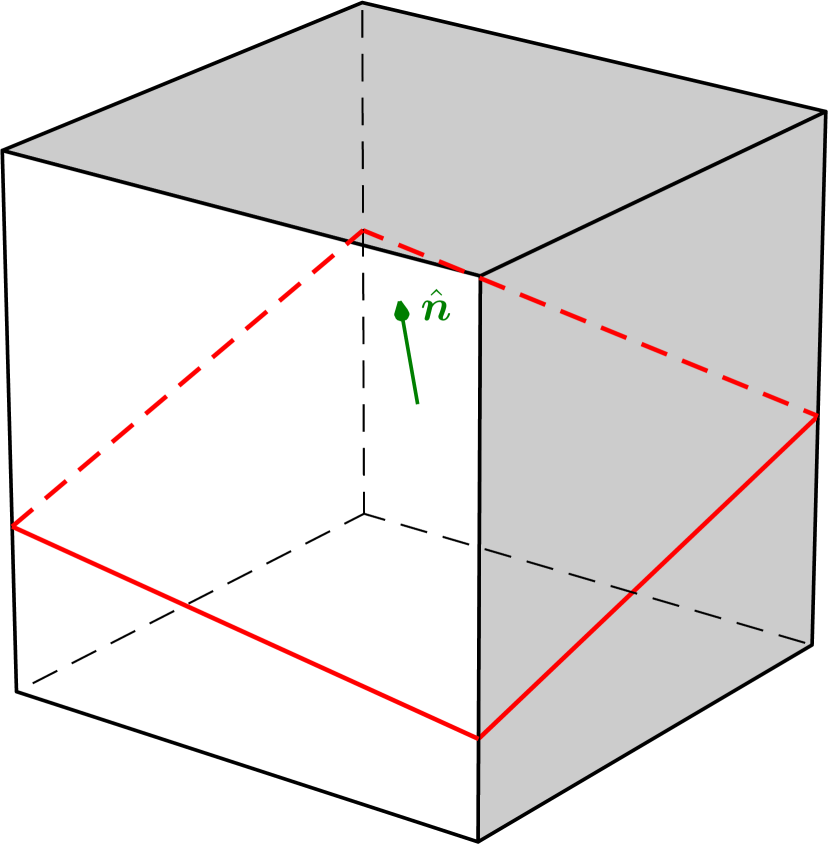
We store a flag in each cell marking it as either uncovered (normal), covered (ignored), or cut. In the latter case, additional data is stored within the cell, so that we can take geometrical information into account for computations in that cell. Since we only consider single-valued cut cells, only four numbers are necessary to uniquely define the cut cell, namely the three components of the boundary surface unit normal plus the volume fraction of fluid within the cell. We orient so that it points into the fluid domain, and let for covered cells and for uncovered ones. Although these quantities describe the cut cell, several helpful additions are available in the EB framework provided by AMReX, such as the uncovered area fractions on each face, the volume centroid of the fluid, and the area and centroid of the embedded boundary. Figure 1 illustrates the cut cell and the relevant quantities for our computations. For details on the EB implementation, we refer to the AMReX documentation, and for an explanation of how EB data is computed from a signed distance function, the reader is referred to the paper by Gokhale et al. Gokhale, Nikiforakis, and Klein (2018b)
All variables in our simulations are stored at the same cell positions, regardless of the cell type. This has the strong advantage of allowing us to avoid altering computational stencils for calculating extrapolated values on faces or approximating gradients based on neighbouring cells which are cut. We only need to worry about the cut cells themselves, which can have covered (and thus undefined) neighbours. The EB tools built in to the linear solvers for systems of linear equations (solutions to the Poisson equations) are based on the work of Johansen and Colella Johansen and Colella (1998).
III.2.1 Flux computations
Our main challenge algorithmically (apart from the linear solves, for which AMReX has built-in EB support) is to successfully compute the derived quantities within each cut cell, i.e. the convective term , the rate-of-strain tensor magnitude , the apparent viscosity and the viscous term . It is crucial that this is done in a manner which avoids time step constraints resulting from small cut cell volumes.
Let us first consider terms which can be written as the divergence of a flux , i.e.
| (23) |
For these, we utilise the flux redistribution technique for embedded boundaries as developed by Colella et al. Colella et al. (2006); Graves et al. (2013). Applying the divergence theorem to a cut cell control volume, we find that
| (24) |
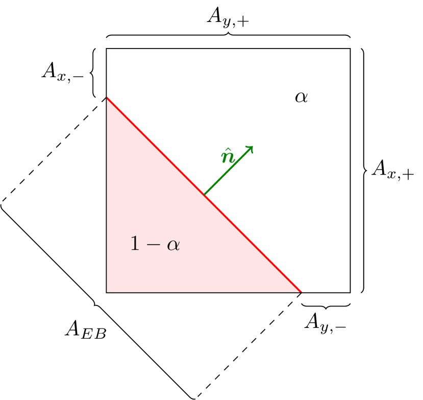
is a conservative estimate of . Here, is the cell volume, is the number of faces (EB or otherwise) enclosing the cell, and is the uncovered surface area of the face , while is its normal vector. For all non-EB faces, we can evaluate the flux tensor just as for uncovered cells, since physical variables are stored at cell centres. Consequently, the slope computation and upwinding procedures do not need to be altered for EB cells except that one-sided upwinding is applied in the case of covered neighbouring cells. In other words, we just need to use the EB information to extrapolate to the uncovered face centroid and multiply it by the corresponding face area. Subscripting fluxes and area fractions in direction by at one end and at the other, (24) can be written
| (25) |
and the only special consideration required is the evaluation of the flux tensor at the EB centroid, . Figure 2 displays these fluxes in a 2D slice of the cut cell.

The downside of the conservative flux as computed in (25) is that the so-called small cell problem arises in the explicit temporal discretisation LeVeque (1988a, b). The time step size is restricted since it is proportional to , which can be arbitrary small in cut cells. In order to circumvent this, we define a non-conservative approximation to the divergence as an average of the conservative approximations in the neighbourhood of the cell,
| (26) |
We define the neighbourhood as the set
| (27) |
i.e. all uncovered or cut cells whose index vector components differ by at most one from , except cell itself. A linear hybridisation of the conservative and non-conservative flux approximations is then given by
| (28) |
Note that this hybrid flux approximation has the desired behaviour in the limits of , and removes the effect of the local volume fraction on the time step size.
Although the hybrid flux stabilises the CFL restriction, it does not strictly enforce conservation. The excess material lost or gained due to the usage of (28) rather than (25) is
| (29) |
and this excess must be redistributed back to the cell neighbours. This is done with the use of weights which quantify the fraction of redistributed to cell , and which must satisfy for strict conversation. We use the simple weights
| (30) |
which are actually independent of . The final, discrete approximation to the divergence operator is thus
| (31) |
III.2.2 Convective term
By the chain rule, we have
| (32) |
where the last equality holds due to the incompressibility constraint in (3b). Seeing the convective term as the divergence of a tensor flux, , we can apply the procedure outlined above in order to compute the convective term in EB cells. Note that we enforce an inhomogeneous Dirichlet condition on at all EB walls, so that the components of the convective flux tensor are all zero there: . As such, we do not need to make any special considerations for the convective fluxes at embedded boundaries. This is in contrast to the viscous wall fluxes, which we will deal with next.
III.2.3 Viscous term
The flux tensor arising from the viscous term is , which can be non-zero on the EB surfaces. We therefore need a procedure to compute the viscous wall flux at the EB surface centroid , which is given relative to local cut cell coordinates, where the cell centre is the origin. To this end, we compute the gradient of each velocity component along the EB surface normal vector . In order to achieve this, we utilise AMReX’ built-in biquadratic interpolation routine to find the value of at two points located at distances and from the EB surface centroid . Figure 3 illustrates the interpolation points for an example cut cell.
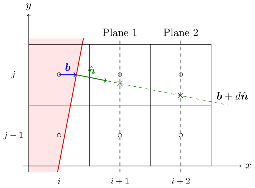
We start by finding which is the largest component of the surface normal vector. The biquadratic interpolation will be done in planes where the corresponding coordinate is held fixed. Consider the case when , as in figure 3. In order to make sure that we are moving away from the EB, we let and define the interpolation points as those where the line intersect the planes and . The corresponding distances from are
| (33) |
We can thus find the and coordinates, and utilise biquadratic interpolation to obtain velocity values based on the 9 nearest points in the plane. Denoting the interpolated velocities by and , and allowing a prescribed velocity on the boundary (zero throughout this paper), (54) gives the normal derivative as
| (34) |
All components of the velocity gradient are now available by taking the projections of in the relevant Cartesian direction, i.e. multiplying by the corresponding component of . We can thus compute , and finally in the cut cell.
III.2.4 Strain rate tensor and apparent viscosity
Since our aim is to accurately capture the flow patterns of fluids with apparent viscosity functions which depend strongly on the magnitude of the rate-of-strain tensor, it is essential that we can compute the components of the velocity gradient tensor to second-order accuracy. The procedure outlined for the viscous wall fluxes above is tailored for computing the values on EB walls, but in the present case we require them at cell centres. In order to circumvent the problem of covered neighbour cells, we adjust the stencil used for difference estimation. Similarly to in the previous subsection, we consider a function whose values we know at three points , with the alteration that but the points have equal spacing . According to (54), the gradient of a quadratic polynomial fit to these points is given by
| (35) |
We can thus evaluate the gradient of the function at the given points to second order accuracy with simple coefficients, since
| (36a) | ||||
| (36b) | ||||
| (36c) | ||||
In order to evaluate the velocity gradient tensor in cut cells, we simply check whether the neighbouring cells in each direction are covered, and if so, utilise a one-sided quadratic difference estimator rather than the central one. Consequently, we are only fishing for values in well-defined cells. With the estimates for velocity gradient components in place, we can evaluate the cell-centred rate-of-strain magnitude and apparent viscosity directly.
IV Verification
Before evaluating the methodology for genuinely three-dimensional viscoplastic flows, we need to ensure that the underlying incompressible flow solver has the desired order of accuracy by performing grid convergence studies for problems with known solution. Furthermore, we verify that the embedded boundaries work as expected by computing the solution to a Bingham Poiseuille flow in a cylinder.
IV.1 Spatio-temporal convergence study: Taylor-Green vortices
In order to demonstrate spatio-temporal second order convergence of the presented algorithm, we consider the unsteady Taylor-Green vortices in a Newtonian fluid, for which an analytical solution exists. The computational domain is , periodic boundary conditions are applied on all faces, and we take as the maximum of the initial velocity distribution. We obtain dimensionless variables by scaling lengths by , velocities components by , time by and pressure by the kinetic energy density . The Taylor-Green solution is then
| (37a) | ||||
| (37b) | ||||
| (37c) | ||||
where we have introduced the Reynolds number .
For a series of spatial resolutions, characterised by the amount of cells, , in each direction, our system is advanced to the time with . The resulting velocity field is subtracted from the analytical solution in each cell, and we denote this residual . For two meshes with resolution and , the convergence rate of our numerical method can be computed as
| (38) |
where is an appropriate function norm, typically one of
| (39a) | |||
| (39b) | |||
| (39c) | |||
Table 2 shows how the convergence rate for our solver approaches two in the discrete version of all these norms as grows, as expected.
| 32 | ||||||
|---|---|---|---|---|---|---|
| 64 | ||||||
| 128 | ||||||
| 256 | ||||||
| 512 |
IV.2 Convergence study for viscoplastic fluid
In order to evaluate the convergence of our code for viscoplastic fluids, we consider plane Poiseuille flow between parallel plates separated by a width , with the plane lying halfway between them. Poiseuille flow is driven by a constant pressure gradient applied in the direction of flow, which is aligned with the parallel plates. Scaling distances by and velocity by the maximum velocity of an unregularised Bingham fluid, the analytical solution at steady-state is
| (40) |
Here, we have introduced the dimensionless length
| (41) |
which separates the flow into yielded and unyielded regions, i.e. represents the yield surface. Note that since we have chosen to fix the maximum dimensionless velocity to unity, is the only free variable in the system, and represents the relative strength of the yield stress to the applied pressure gradient. For the sake of completeness, we note that the characteristic velocity is given by
| (42) |
Although (41) gives us the analytical solution for a Bingham fluid, it would not be correct to use for convergence analysis since the Papanastasiou regularisation which we are employing is not an equivalent formulation. We have therefore derived the analytical solution for a Papanastasiou regularised Bingham fluid, as shown in appendix B. It is given by
| (43) |
where , and where is the Lambert function, which is also known as the product logarithm, since it is defined as the solution to .
| 0 | 16 | ||||||
|---|---|---|---|---|---|---|---|
| 32 | |||||||
| 64 | |||||||
| 128 | |||||||
| 0.1 | 16 | ||||||
| 32 | |||||||
| 64 | |||||||
| 128 | |||||||
| 256 | |||||||
| 0.2 | 16 | ||||||
| 32 | |||||||
| 64 | |||||||
| 128 | |||||||
| 256 | |||||||
| 0.5 | 16 | ||||||
| 32 | |||||||
| 64 | |||||||
| 128 | |||||||
| 256 |
We emphasise that the newly derived analytical solution given by (43) takes into account the effect of the regularisation parameter on the analytical solution, so that that factor is removed from the numerical algorithm in our convergence study. We therefore use a moderate , which in any case is small enough to capture the yield stress effects on this simple problem, and vary the amounts of grid points over the channel width. The experiment is repeated for several values of , since we expect the condition number of the numerical problem to increase with the Bingham number. As seen in table 3, the numerical solution converges to (43) with increasing spatial accuracy for all values of . Since the analytical solution is parabolic for the Newtonian case, we achieve a perfect second order convergence rate, but is drops to slightly lower than two as the yield stress increases. This is as expected, and the solution in the unyielded region (which is undefined for Bingham fluids) converges slowest. Following the convergence analysis of Olshanskii Olshanskii (2009), table 4 shows the corresponding convergence rates when we only consider the yielded region (), which are much better even for . The -norm is the same, since it measures the maximum error throughout the domain, which is immediately outside the yield surface in all cases. Although the strongly non-linear viscosity function poses a significant numerical challenge, our algorithm performs well. Even more rapid convergence could possibly be achieved through the use of convergence acceleration methods such as those discussed by Housiadas Housiadas (2017).
| 0.1 | 16 | ||||||
|---|---|---|---|---|---|---|---|
| 32 | |||||||
| 64 | |||||||
| 128 | |||||||
| 256 | |||||||
| 0.2 | 16 | ||||||
| 32 | |||||||
| 64 | |||||||
| 128 | |||||||
| 256 | |||||||
| 0.5 | 16 | ||||||
| 32 | |||||||
| 64 | |||||||
| 128 | |||||||
| 256 |
V Evaluation
In order to properly evaluate the capabilities of our code, we need to simulate test cases which exhibit fully three-dimensional effects which are characteristic of yield stress fluids. A widely discussed case is that of bodies moving at constant speed through a Bingham fluid. Such bodies are fully encapsulated by a so-called yield envelope, separating the unyielded bulk material from an interior recirculating flow. This interior flow has a unique topology owing to the viscoplastic nature of the fluid, and has been widely studied for two-dimensional Ansley and Smith (1967); Beris et al. (1985); Blackery and Mitsoulis (1997); Liu, Muller, and Denn (2002); Tokpavi, Magnin, and Jay (2008); Chaparian and Frigaard (2017); Koblitz, Lovett, and Nikiforakis (2018b) and axisymmetric three-dimensional Prashant and Derksen (2011); Chen et al. (2016) shapes.
V.1 Cylinder moving through Bingham fluid
Although creeping flow past a sphere in a viscoplastic fluid was investigated first Ansley and Smith (1967), the simpler case is that of an infinitely long circular cylinder. This is due to the fact that only a thin slice in 3D is required for comparisons with two-dimensional reference results, but also because the viscoplastic effects are more dominant due to the extended geometry. Consequently, there is no ambiguity regarding the resulting shape of yield surfaces. The problem was first considered by Adachi and Yoshioka Adachi and Yoshioka (1973), who used variational principles and slip-line analyses to estimate the relevant drag effects. Randolph and Houlsby Randolph and Houlsby (1984) used plasticity theory to investigate the same problem in the context of pile pressure in cohesive soil. Two excellent references which utilised numerical simulations to explore the problem are the papers by Mitsoulis Mitsoulis (2004) and Tokpavi et al. Tokpavi, Magnin, and Jay (2008), in which the flow around a highly resolved 2D quadrant surrounding the cylinder was simulated with Papanastasiou regularisation schemes. The former investigated the influence of wall effects for creeping flow, and found that it was small for medium to large Bingham numbers, while the latter extended the parameter ranges and analysis of the problem. They showed that the occurrence of characteristic dips in the yield envelope fore and aft of the cylinder is clearly prominent for Bingham fluids, in addition to small unyielded caps attached to the poles of the cylinder and rigidly rotating unyielded plugs in its equatorial plane. The same has been demonstrated by Chaparian and Frigaard Chaparian and Frigaard (2017) by using an augmented Lagrangian approach, which captures the yield surface without regularisation. They also show how slip line field theory captures the yield envelope and polar caps well, but is ill-suited for the equatorial plugs. It is also worth mentioning that there have been a number of studies with multiple cylinders in various collinear configurations, all showing similar large-scale features Liu, Muller, and Denn (2003); Prashant and Derksen (2011); Koblitz, Lovett, and Nikiforakis (2018b). Since the problem is essentially two-dimensional due to its planar symmetry, we expect to see the same yield surface shapes as the aforementioned authors, even though our code is fully three-dimensional.
We thus consider an infinitely long circular cylinder, where the direction of flow (along the unit vector ) is perpendicular to the cylinder axis (). The computational domain is , where is the length of the computational domain along the cylinder and is its diameter, which we take as the characteristic length scale. In the following simulations, we have used and periodic boundary conditions in the -direction. Rather than imposing a constant velocity on the cylinder, we keep it fixed and instead let everywhere initially and at the domain boundaries as the simulation progresses. This means that the cylinder is falling with the same speed () in the reference frame where the bulk fluid is at rest. Periodic boundary conditions are imposed in the axial direction of the cylinder.
Apart from the regularisation parameter , there are two dimensionless numbers which govern the flow, namely the Reynolds number
| (44) |
and the Bingham number
| (45) |
which quantifies the relative strength of yield stress to viscous stress. We are interested in the creeping flow regime with a high degree of viscoplasticity, so we let . As numerical parameters, we let and . We expect these choices to be suitable for capturing the relevant flow features in this problem, based on the work of Liu et al. Liu, Muller, and Denn (2002) and our own results in subsection V.2.
For flow past bodies, quantitative comparisons with results from the literature are obtained through the computation of a drag coefficient, which is the ratio of the total drag force on the body compared to a reference force. For the cylinder, we take the reference as the product of the characteristic stress and the cross-sectional area of the cylinder . Denoting the boundary of the body by , the drag force is given by the surface integral
| (46) |
while the drag coefficient is
| (47) |
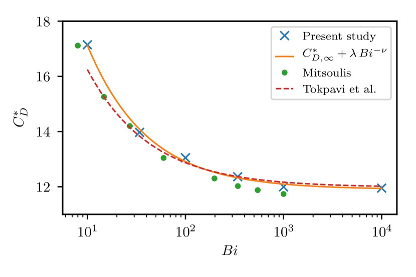
The integral in (46) is computed using numerical quadrature. In order to verify the drag force calculations, we initially perform a simulation with a Newtonian fluid, resulting in a computed drag coefficient equal to 21.8128. For comparison, Faxén’s formula as given by (62) for a semi-analytical drag coefficient yields a value of 21.9642, i.e. a relative discrepancy of 0.69%. By driving the system to steady-state for various Bingham numbers, we can compare our results with others which have been published in the literature. Figure 4 shows how the ratio gradually approaches the asymptotic value as Bi grows large. The numerical results of Mitsoulis Mitsoulis (2004) and Tokpavi et al. Tokpavi, Magnin, and Jay (2008) are overlain our own, and the behaviour similar. Our results are closest to the trend line by Tokpavi et al., which they fit to the function
| (48) |
Our data has been fit to the same function, and we have also computed the gravity yield number
| (49) |
where is the gravitational acceleration and is the density difference between the solid cylinder and surrounding fluid. This dimensionless number is the smallest ratio of yield stress to gravitational stresses which obstructs the solid from falling through the fluid, and for the particular configuration at hand, we have Mitsoulis (2004). Table 5 shows our quantitative results alongside those by other authors.
| Reference | ||||
|---|---|---|---|---|
| Adachi & Yoshioka Adachi and Yoshioka (1973) | 10.28 | 0.09728 | ||
| Randolph & Houlsby Randolph and Houlsby (1984) | 11.94 | 0.08375 | ||
| Mitsoulis Mitsoulis (2004) | 11.70 | 0.08547 | ||
| Tokpavi et al. Tokpavi, Magnin, and Jay (2008) | 11.98 | 0.08347 | 20.43 | 0.68 |
| Present study | 11.90 | 0.08403 | 26.99 | 0.7131 |
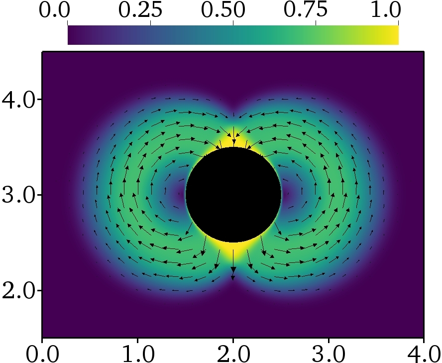
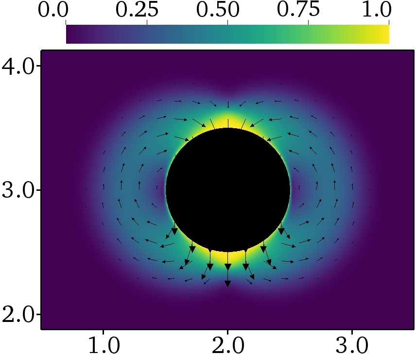
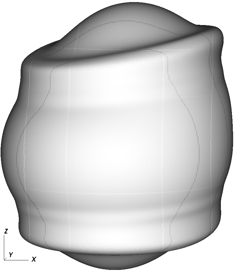
In addition to computing drag coefficients, there is a lot of insight to be gained from visualising different metrics of the flow field. Figure 5 therefore illuminates the resulting flow field through plots of several different variables, for the case with . The Bingham number is chosen to match that in the study by Liu, Muller and Denn Liu, Muller, and Denn (2002), where it is stated that this number is large enough to diminish any outer boundary wall effects for the given choice of domain size. The upper left plot, (a), shows the relative speed with velocity vectors overlaid. A distinct boundary is visible, enclosing a region of non-zero relative velocity surrounding the cylinder. This boundary represents the yield envelope of the body. The velocity vectors indicate a recirculating flow, sweeping material away from the front of the travelling cylinder to the rear in a wide, circular arc. This results in slowly moving material either side of the cylinder, in addition to material travelling at the same speed as the cylinder at the polar caps. These observations are indicative of the expected unyielded plugs rotating at the equator and clinging to the polar caps.
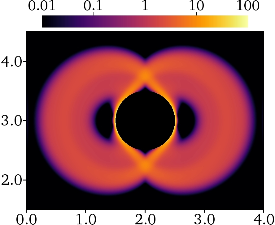
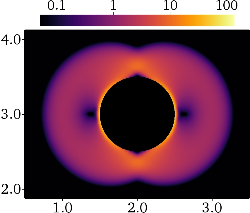
In the upper right plot, (b), the magnitude of the rate-of-strain tensor is shown with logarithmic scaling for the colormap. This plot properly elucidates the low-strain regions of unyielded fluid, and confirm the existence of rigidly rotating equatorial plugs and unyielded material attached to the polar caps, as implied by the velocity distribution. Note that although the yield surface is characterised by the contour for ideal Bingham plastics as given by (5), the regularised version (6) leads to a yield surface given by
| (50) |
where we recall that is the Lambert function. With the current parameter values, (50) gives a yield surface characterised by s-1, which is why we have used s-1 as the lower limit of the colormap.
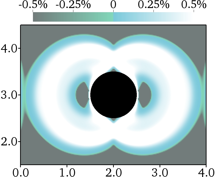
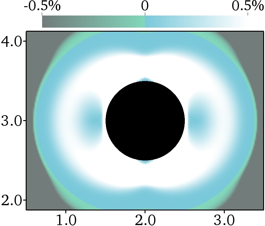
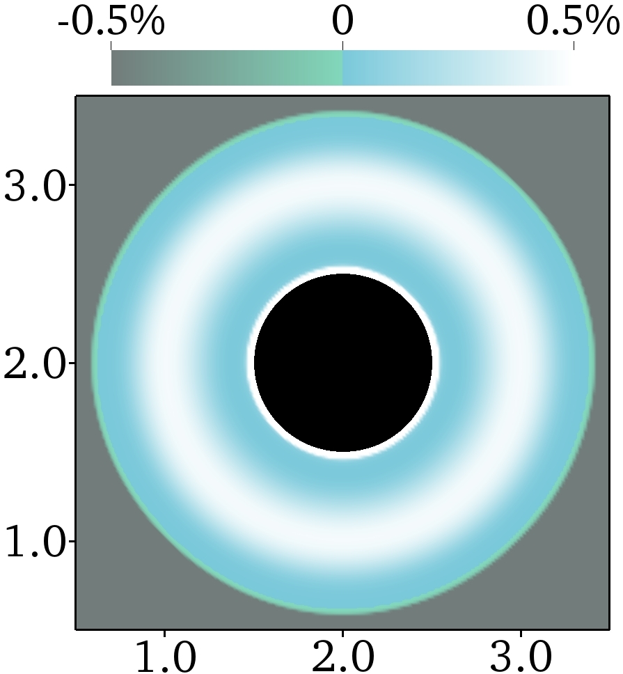
In order to illustrate the location of the yield surface, an option would be to draw the contour where the stress magnitude is equal to . However, as discussed previously in the literature, there is instability near this stress value which means that a better measure of the fully converged yield surface is the contour Olshanskii (2009), where is some small parameter of the order . This is because the solution converges much faster in the yielded region than in the unyielded ones. On the other hand, Treskatis argues that a better visual investigation of the yield surface is obtained by plotting the relative deviation from the yield surface, , restricted to some small range around zero Treskatis, Moyers-Gonzalez, and Price (2016). In this manner, we avoid the introduction of systematic error through overestimation of the unyielded regions. Note that this must be done using a colormap which changes abruptly at zero, as seen in figure 5(c). The transition is somewhat diffuse, but all the expected unyielded regions (envelope, rotating plugs and polar caps) are clearly captured where the stress deviation is negative. The actual yield surface is located somewhere in the transition from blue to white.
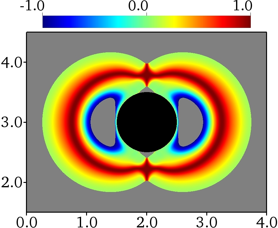
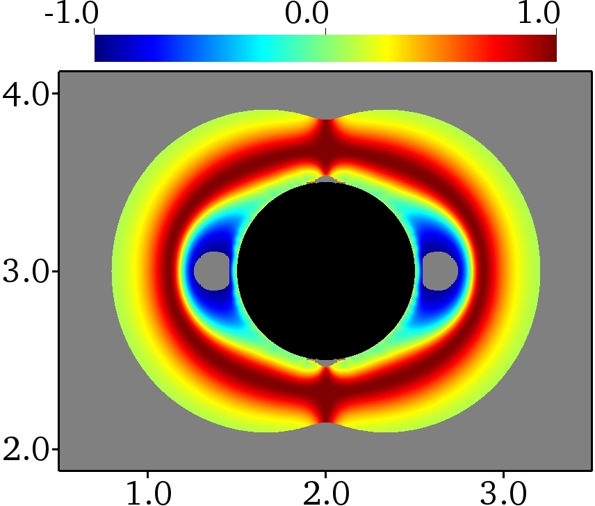
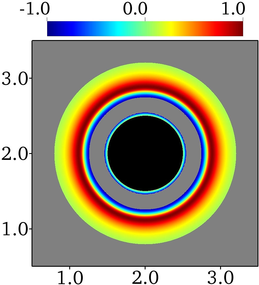
Finally, in figure 5(d) we have plotted a flow topology parameter which is a normalised invariant of the velocity gradient tensor. It indicates the relative strengths of the strain rate and the vorticity Davidson (2015); De et al. (2017),
| (51) |
This parameter accurately describes the nature of different parts of the flow regime, since values of equal to , 0 and 1 correspond to pure rotation, shear and extension, respectively. As expected, we observe pure rotation around the unyielded plugs on the equatorial line of the cylinder. Adjacent to areas of rigid rotation, and near the cylinder, shear flow is evident. This is also the case near the yield envelope. In fact, these two shearing regions represent two distinct cases of viscoplastic boundary layers, as discussed originally by Oldroyd in 1947 Oldroyd (1947b) and more recently by Balmforth in his newly published lecture notes Balmforth (2019). We also point the interested reader to discussions surrounding viscoplastic boundary layer around particles in some of the other works which have already been mentioned Beris et al. (1985); Tokpavi, Magnin, and Jay (2008); Chaparian and Frigaard (2017). Finally, a belt of purely extensional flow surrounds the cylinder, rotating plugs and polar caps. Note that in this plot, the yield surfaces masked out in grey are computed with . This allows us to verify that we recover the same yield surface shapes as those computed in the references Tokpavi, Magnin, and Jay (2008); Chaparian and Frigaard (2017), when using the same visualisation procedure.
V.2 Sphere moving through Bingham fluid
Since the cylinder test case allows for direct comparisons with two-dimensional simulations, it is a good test case for verifying the interplay between yield stress rheology and the embedded boundaries. On the other hand, it does not exhibit any genuinely three-dimensional effects, and for many real-world scenarios an infinite cylinder is not a realistic representation of the actual bluff bodies. We therefore investigate the flow around a sphere in the same configuration, retaining its diameter as the characteristic length scale, but extending the domain to in the -direction. This problem has been analysed by several authors previously Ansley and Smith (1967); Beris et al. (1985); Blackery and Mitsoulis (1997); Liu, Muller, and Denn (2002); Prashant and Derksen (2011); Chen et al. (2016), but it still warrants further attention due to gaps relating to important viscoplastic flow features. In particular, claims about how specific parts of the yield surface depend on spatial resolution and regularisation parameter are not consistent. Furthermore, few of them were based on three-dimensional simulations, and those that were tended to be hampered by low spatial resolution, making it difficult to draw any conclusions regarding the shape and extent of the yield surface.
Ansley and Smith first considered the problem in 1967, and proposed a yield surface based on slip line field theory. This included dips in the yield envelope and polar caps Ansley and Smith (1967). Although it was a great contribution, they conceded that the qualitative shape of the yield surface could not be supported by direct evidence. Beris et al. phrased the problem as a free boundary problem at the yield surface, and performed 2D simulations with a priori estimates of its location Beris et al. (1985). They captured the envelope dips and polar caps, and reported an equatorial torus-shaped region with low strain rate. Its motion was described as close to the sum of rigid translation in the direction of flow and solid body rotation, but they aptly noted that perfectly rigid rotation is not possible in the configuration, except exactly in the equatorial plane. This is due to the rotated strain field around the equator of the sphere. Liu et al. Liu, Muller, and Denn (2002) computed 2D results in a quadrant using Papanastasiou regularisation and finite elements on a body fitted mesh. They reported the existence of both polar caps and a equatorial torus, although the latter is unphysical according to the arguments put forth by Beris et al. They showed that the plug regions shrank with decreasing regularisation parameter, but could not infer the limiting behaviour. More recently, three-dimensional simulations in the framework of lattice Boltzmann techniques have been published, utilising a dual viscosity model Prashant and Derksen (2011) and Papanastasiou regularisation Chen et al. (2016). However, the resolution for these simulations was low (), so it is difficult to draw accurate conclusions regarding the yield surface shapes.
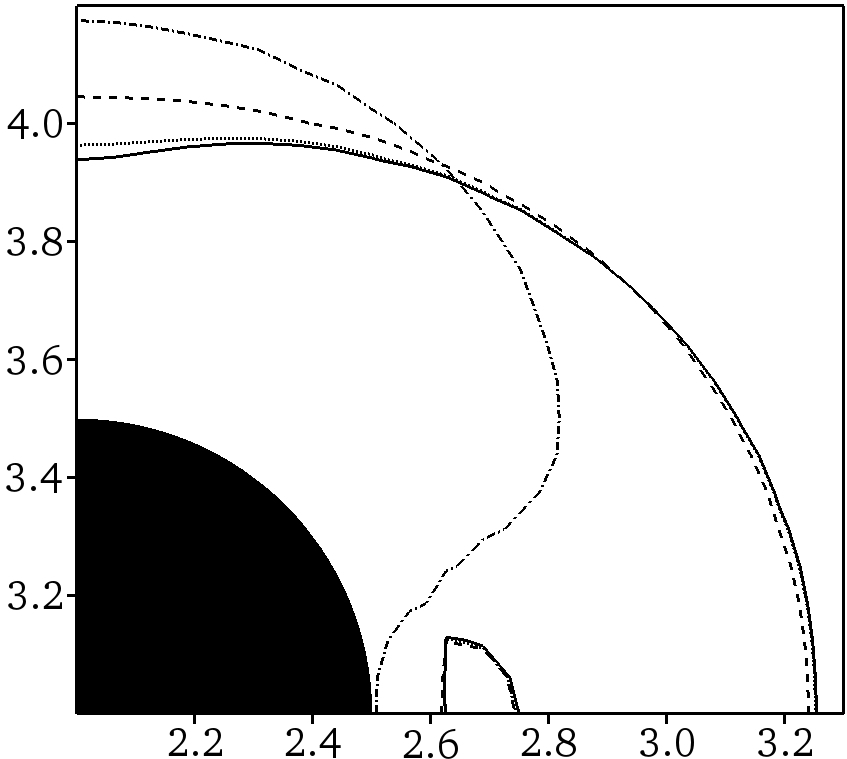
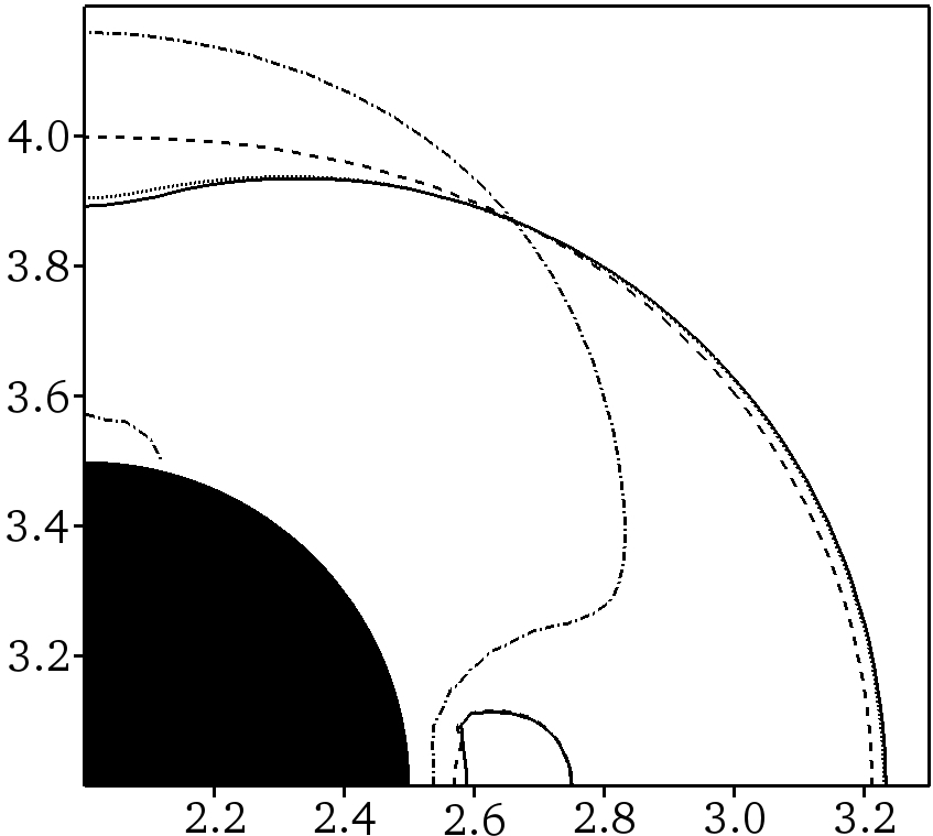
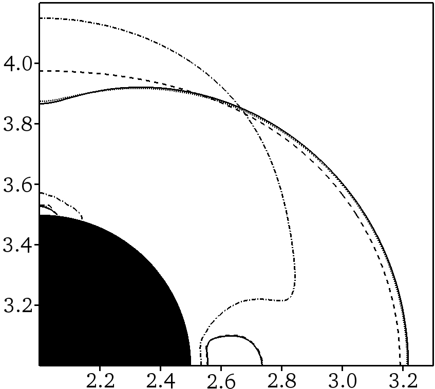
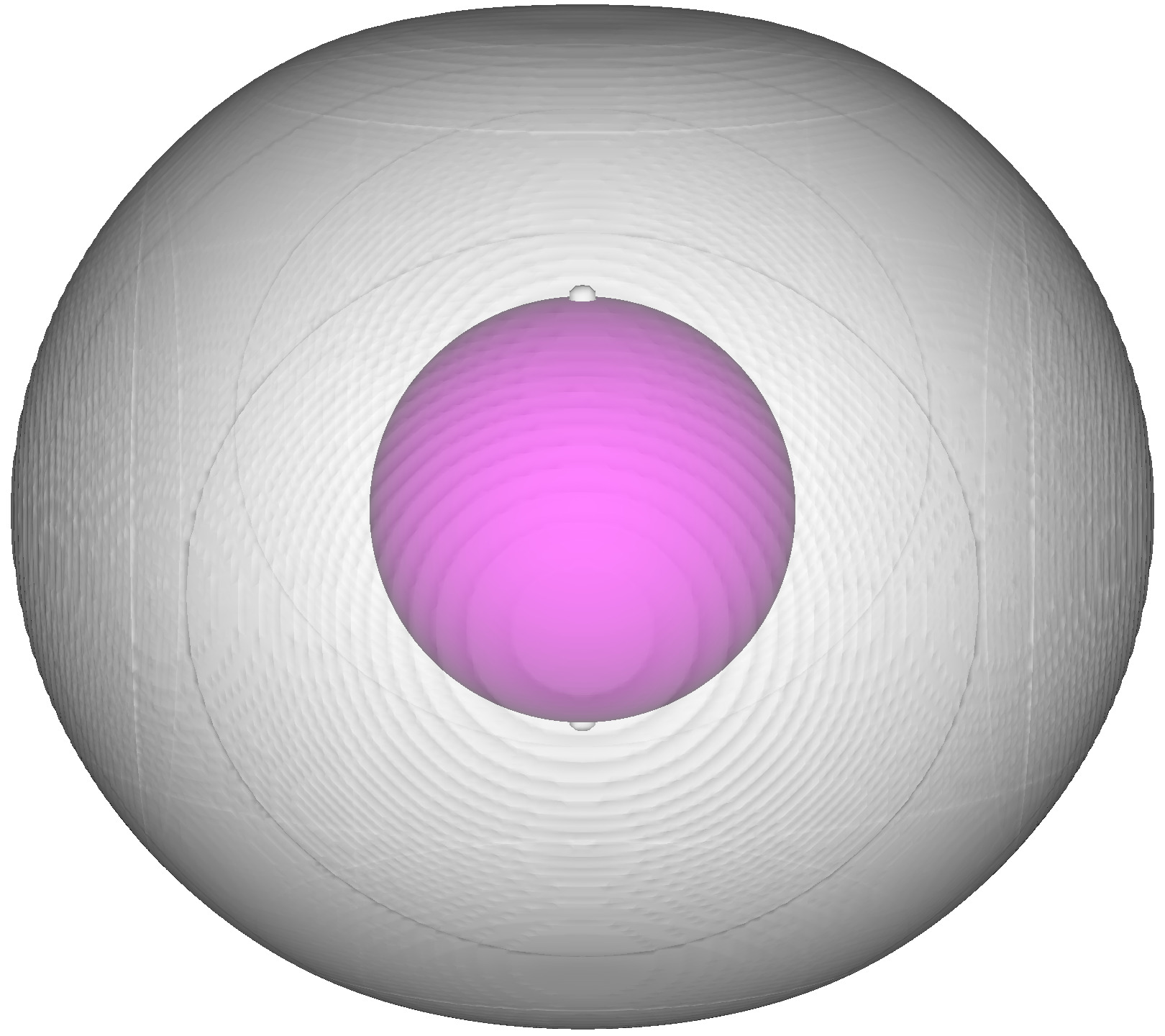
The two parameters which determine the yield surface for a given Bingham number, are the regularisation parameter and the spatial resolution as given by . Similarly to what was done in the paper by Liu et al. Liu, Muller, and Denn (2002), in Figure 6 we plot the computed yield surfaces in the upper right corner of the plane , which goes directly through the sphere, for a range of values. However, we also consider three different mesh resolutions, in order to separate the effects of the two parameters. It is clear that both parameters must have acceptable values in order for the solution to converge as expected. Without a small enough regularisation parameter (at least ), the yield envelope dips and low-strain equatorial plugs are not captured, whereas a low spatial resolution results in unresolved polar caps. We note that the unphysical torus-shaped yield surface at the equator is apparent also in our simulations, but this is due to the utilisation of in the visualisation of the yield surface, as explained below. In the remainder of this section, we let and .
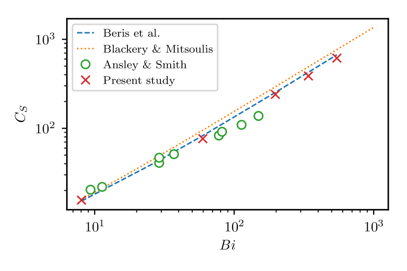
For the case of a sphere, the reference force for the computation of the drag coefficient is the Stokes force Stokes (1851) that acts on a sphere falling in an infinite Newtonian medium. The Stokes drag coefficient is thus
| (52) |
Figure 7 shows our results alongside previously published data in the literature. We have included the original computational results by Beris et al. Beris et al. (1985) and Blackery and Mitsoulis Blackery and Mitsoulis (1997) as dashed and dotted lines, respectively, and have also overlaid the experimental results of Ansley and Smith Ansley and Smith (1967). As is evident, our computed values for the Stokes drag coefficient lie within the same range as the references, and match the results of Beris et al. most closely.
In figure 8, we show plots of the same variables as those in figure 5 for the cylinder. There are several noteworthy points to make about the differences between the two cases. Firstly, the overall size of the yield envelope is significantly smaller for the sphere than the cylinder, both in the direction of flow and in the -plane. Secondly, the unyielded regions within the envelope are much smaller. Both of these observations are as expected, since the axial symmetry of the sphere causes reduced shearing effects in the plane. Equivalently, the extended cylinder enhances shearing in the plane, leading to the larger unyielded regions and genuine rigid body rotation. Finally, the relative stress deviation plot (c) proves that there aren’t any regions in the equatorial torus where the stress is actually below the yield stress threshold. Although the stress gets extremely close to the yield threshold in these areas of low strain, there is no evidence of a genuinely unyielded region, since the relative stress plot stays blue. The diffuse interfaces in this plot shed some light on why the torus-shaped plug is present in some papers and not others: it is severely close to the threshold value without actually reaching it, and without a sharp transition near it. Thus, the benefits of the visualisation strategy introduced by Treskatis becomes clear: the plot in (c) shows in details what the stress deviation looks like near the yield surface, while the well-known masked out contour in (d) oversimplifies the case. This is all in agreement with the original arguments put forth by Beris et al. Beris et al. (1985) Figure 9 shows the last two plots through the slice , i.e. perpendicular to the flow direction, but still through the centre of the sphere.
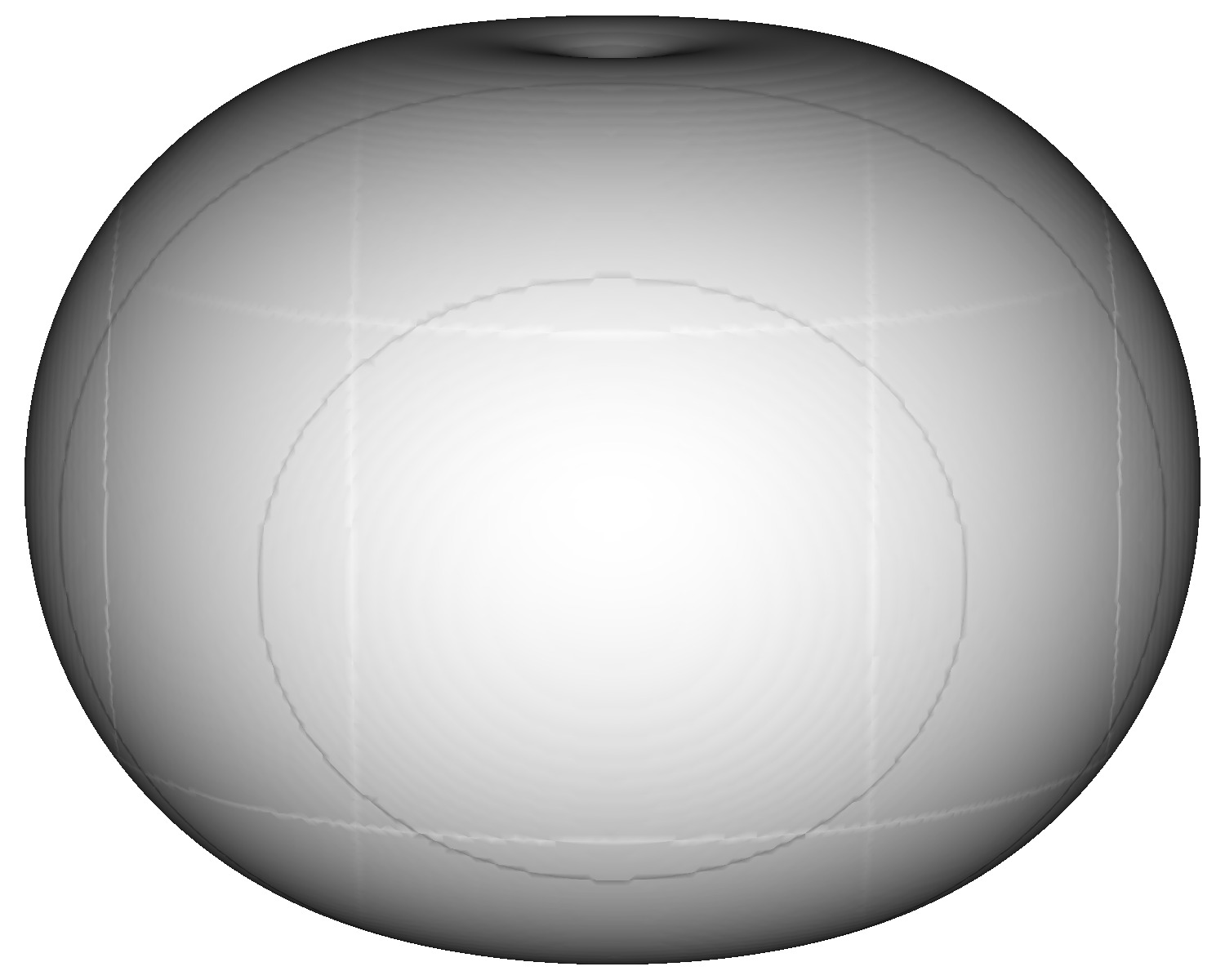
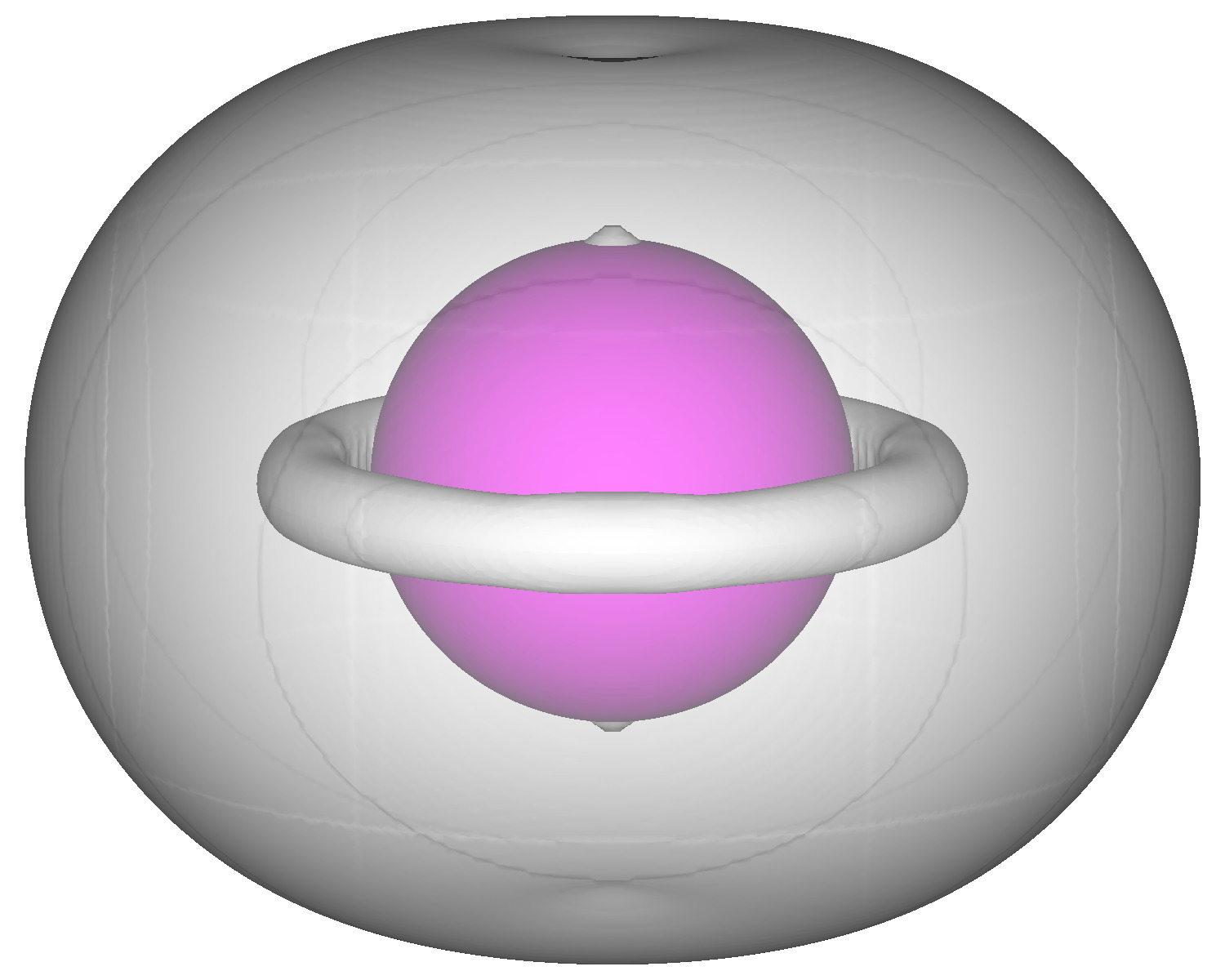
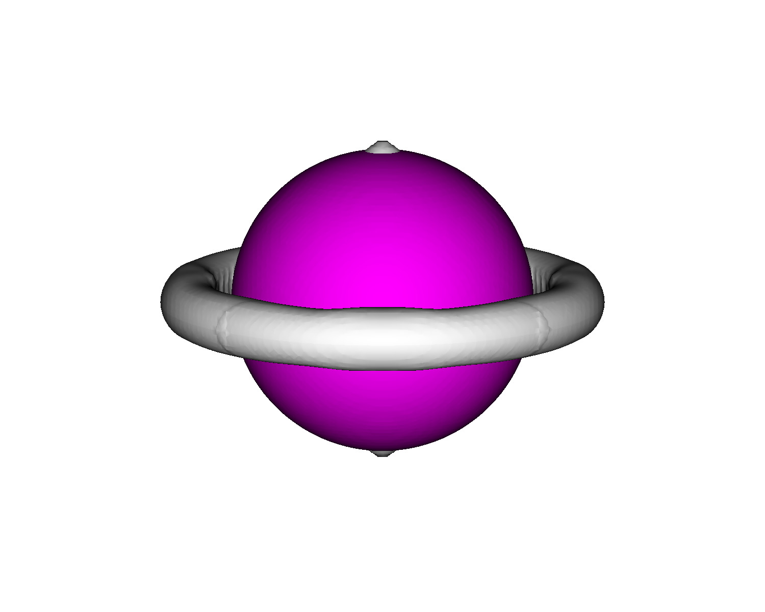
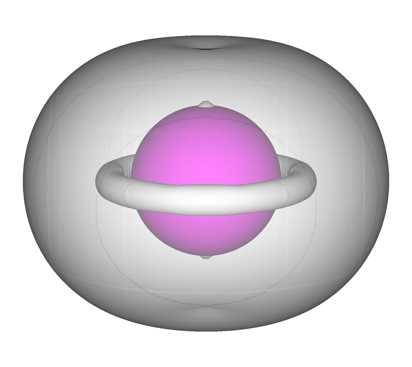
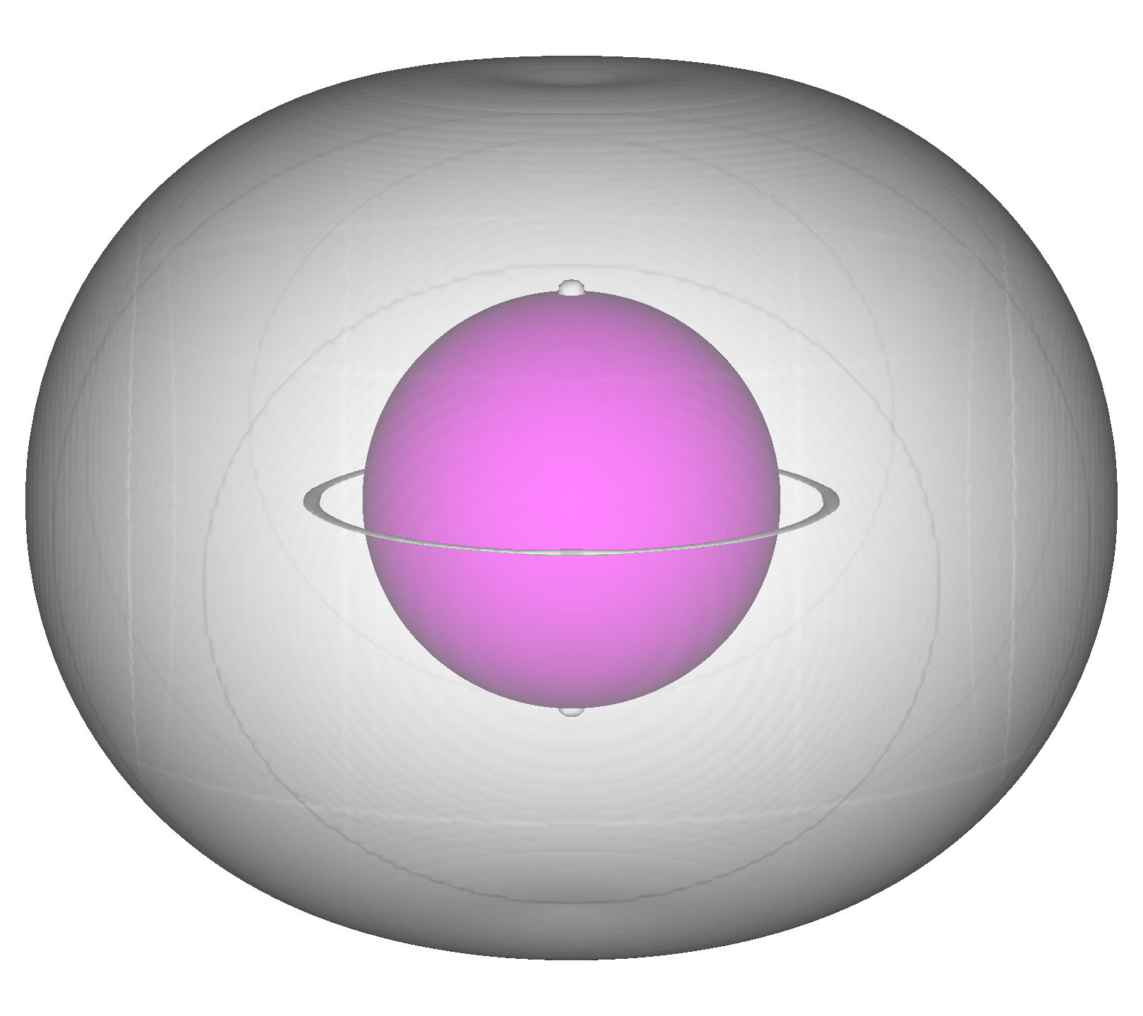
Finally, in figures 10 and 11, we visualise three-dimensional stress contours in the vicinity of the sphere. In the former, the yield surfaces are all computed with . Since the yield envelope fully encloses the sphere and plug regions, its opacity is reduced from subfigures (a) to (c), in order to reveal the shape of the enclosed yield surfaces. This kind of visualisation is entirely novel to the best of our knowledge, and gives a richer picture of the yield surface topology. Since there is no body-fitted mesh or assumption on symmetry in the flow, this type of simulation opens a range of possibilities for investigating flow patterns and yield surfaces in complex configurations. The effect of reducing is illustrated in figure 11, and confirms that the toroidal yield surface at the equator disappears in the limit , at the cost of poorer resolution for the yield envelope.
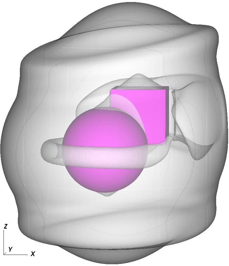
V.3 Non-trivial particle shape
As a final demonstration, we replace the sphere by an object which is the union of a sphere and cube, and orient it so that the flow field becomes asymmetrical. This means that a three-dimensional representation is necessary to capture the fluid dynamics. To be precise, the sphere is the same size as in the previous section, but has centre coordinates , while the cube is defined by two points on opposing sides of its main diagonal, in dimensionless units and . We retain the highest resolution settings used for the sphere, i.e. , and . The resulting 3D yield surface, computed with , is shown in figure 12 (Multimedia view). In contrast to figure 10, we reduce the opacity of all the yield surfaces, and not just the enclosing envelope. This is due to the difficulty in separating the locations of the yield surface types by simple rules. Although the stress contours are now much more complex, we can still recognise the expected traits: an enclosing yield envelope surrounding the entire body, in addition to smaller unyielded plugs attached to it at places of low strain rate. In particular, there are caps of unyielded material fore and aft of the object in the flow direction, as well as along the narrow intersection of the sphere and cube. Additionally, the characteristic low-strain rotating region around the sphere’s equator is visible, but it does not continue around the entire object. The free cube sides, which are aligned with the flow direction, only lead to a very narrow boundary layer separating the object from the yield envelope. A video is available online, in which the observer’s point of view is rotated around the object in order to show the yield surface from all polar angles.
VI Conclusions
We have presented a new methodology for simulating highly resolved flow of generalised Newtonian fluids (in particular, viscoplastics) in three-dimensional domains with non-rectangular boundaries. The domain geometry is treated using embedded boundaries, which are applied to viscoplastic fluid computations for the first time. Highly resolved simulations are made possible by implementing the algorithm in AMReX, a high performance library of tools for solving PDEs on structured grids. The solver is robust and efficient, and allowed us to perform simulations of various objects moving at constant relative speed through an infinite volume of Bingham fluid, revealing the shape of the resulting yield envelopes and plug regions. We hope our contribution can prove a useful tool to researchers interested in studying three-dimensional flows of Bingham fluids in non-rectangular domains or around various body shapes.
Acknowledgements.
K. S. would like to acknowledge the EPSRC Centre for Doctoral Training in Computational Methods for Materials Science for funding under grant number EP/L015552/1. Additionally, he acknowledges the funding and technical support from BP through the BP International Centre for Advanced Materials (BP-ICAM) which made this research possible. Finally, he is grateful to Arndt Ryo Koblitz for useful discussions and for sharing his valuable insights.Appendix A Polynomial interpolation
Given a set of real values at data points for , polynomial interpolation seeks to find a polynomial function of degree whose curve passes through each of them. The Lagrange form of the interpolant is given by
| (53) |
so that it’s derivative is
| (54) |
The polynomial interpolant is unique and accurate to order .
Appendix B Analytical solution for Poiseuille flow of a Papanastasiou regularised Bingham fluid
Plane Poiseuille flow of a Papanastasiou regularised Bingham fluid in a channel of width in the -direction is driven by a constant applied pressure gradient in the -direction, resulting in a steady-state solution with non-zero -velocity aligned with the channel plates. The velocity profile is only a function of , and takes its maximum value at the centre of the channel, . The plane is a symmetry plane for the solution, so we solve for . We take as the characteristic length, while the characteristic speed is the maximum of the unregularised analytical solution. Scaling by these, in addition to strain rate and stress , the steady-state governing equations in dimensionless form are
| (55a) | ||||
| (55b) | ||||
| (55c) | ||||
Here, the Bingham number is . Since the only non-zero velocity component is , the magnitude of the rate-of-strain tensor is . Furthermore, since is monotonically decreasing for , we have . With this information in place, the first component of (55a) is
| (56) |
where is the location of the yield surface in the unregularised Bingham model. Its relationship to the Bingham number (which is superfluous in this description) is
| (57) |
Equation (56) is a separable differential equation for :
| (58) |
For ease of writing, we introduce . The solution to (58) is then
| (59) |
where we have found the explicit solution by use of the Lambert function and the fact that at . Using the no-slip boundary condition , and the identity
| (60) |
direct integration then gives the analytical expression for the velocity profile as
| (61) |
Appendix C Faxén’s formula
As shown by Faxén in 1946 Faxén (1946), the creeping drag force per unit length of a cylinder with diameter moving at speed through the centre of a channel of width filled with a Newtonian fluid with viscosity coefficient , is given by
| (62) |
References
- Saramito and Wachs (2017) P. Saramito and A. Wachs, “Progress in numerical simulation of yield stress fluid flows,” Rheologica Acta 56, 211–230 (2017).
- Mitsoulis and Tsamopoulos (2017) E. Mitsoulis and J. Tsamopoulos, “Numerical simulations of complex yield-stress fluid flows,” Rheologica Acta 56, 231–258 (2017).
- Koblitz, Lovett, and Nikiforakis (2018a) A. Koblitz, S. Lovett, and N. Nikiforakis, “Direct numerical simulation of particle sedimentation in a Bingham fluid,” Physical Review Fluids 3, 093302 (2018a).
- Kanaris, Kassinos, and Alexandrou (2015) N. Kanaris, S. Kassinos, and A. Alexandrou, “On the transition to turbulence of a viscoplastic fluid past a confined cylinder: A numerical study,” International Journal of Heat and Fluid Flow 55, 65–75 (2015).
- Chaparian, Wachs, and Frigaard (2018) E. Chaparian, A. Wachs, and I. A. Frigaard, “Inline motion and hydrodynamic interaction of 2D particles in a viscoplastic fluid,” Physics of Fluids 30, 033101 (2018).
- Roosing, Strickson, and Nikiforakis (2019) A. Roosing, O. Strickson, and N. Nikiforakis, “Fast distance fields for fluid dynamics mesh generation on graphics hardware,” Communications in Computational Physics 26, 654–680 (2019).
- Purvis and Burkhalter (1979) J. W. Purvis and J. E. Burkhalter, “Prediction of critical Mach number for store configurations,” AIAA Journal 17, 1170–1177 (1979).
- Wedan and South (1983) B. Wedan and J. South, Jr., “A method for solving the transonic full-potential equation for general configurations,” in 6th Computational Fluid Dynamics Conference Danvers (1983) p. 1889.
- Clarke, Hassan, and Salas (1986) D. K. Clarke, H. Hassan, and M. Salas, “Euler calculations for multielement airfoils using Cartesian grids,” AIAA journal 24, 353–358 (1986).
- Falle and Giddings (1988) S. Falle and J. Giddings, “An adaptive multigrid applied to supersonic blunt body flow,” Numerical Methods in Fluid Dynamics, III (1988).
- Berger and Leveque (1989) M. Berger and R. Leveque, “An adaptive Cartesian mesh algorithm for the Euler equations in arbitrary geometries,” in 9th Computational Fluid Dynamics Conference (1989) p. 1930.
- Colella et al. (2006) P. Colella, D. T. Graves, B. J. Keen, and D. Modiano, “A Cartesian grid embedded boundary method for hyperbolic conservation laws,” Journal of Computational Physics 211, 347–366 (2006).
- Johansen and Colella (1998) H. Johansen and P. Colella, “A Cartesian grid embedded boundary method for Poisson’s equation on irregular domains,” Journal of Computational Physics 147, 60–85 (1998).
- McCorquodale, Colella, and Johansen (2001) P. McCorquodale, P. Colella, and H. Johansen, “A Cartesian grid embedded boundary method for the heat equation on irregular domains,” Journal of Computational Physics 173, 620–635 (2001).
- Berger (2017) M. Berger, “Cut cells: meshes and solvers,” in Handbook of Numerical Analysis, Vol. 18 (Elsevier, 2017) pp. 1–22.
- Gokhale, Nikiforakis, and Klein (2018a) N. Gokhale, N. Nikiforakis, and R. Klein, “A dimensionally split Cartesian cut cell method for hyperbolic conservation laws,” Journal of Computational Physics 364, 186–208 (2018a).
- Gokhale, Nikiforakis, and Klein (2018b) N. Gokhale, N. Nikiforakis, and R. Klein, “A dimensionally split Cartesian cut cell method for the compressible Navier–Stokes equations,” Journal of Computational Physics 375, 1205–1219 (2018b).
- Sverdrup, Nikiforakis, and Almgren (2018) K. Sverdrup, N. Nikiforakis, and A. Almgren, “Highly parallelisable simulations of time-dependent viscoplastic fluid flow with structured adaptive mesh refinement,” Physics of Fluids 30, 093102 (2018).
- Wachs (2019) A. Wachs, “Computational methods for viscoplastic fluid flows,” in Lectures on Visco-Plastic Fluid Mechanics (Springer, 2019) pp. 83–125.
- Muravleva (2017) L. Muravleva, “Axisymmetric squeeze flow of a viscoplastic Bingham medium,” Journal of Non-Newtonian Fluid Mechanics 249, 97–120 (2017).
- Muravleva (2018) L. Muravleva, “Squeeze flow of Bingham plastic with stick-slip at the wall,” Physics of Fluids 30, 030709 (2018).
- Barnes, Hutton, and Walters (1989) H. A. Barnes, J. F. Hutton, and K. Walters, An introduction to rheology, Vol. 3 (Elsevier, 1989).
- Mewis (1979) J. Mewis, “Thixotropy—a general review,” Journal of Non-Newtonian Fluid Mechanics 6, 1–20 (1979).
- Barnes (1997) H. A. Barnes, “Thixotropy—a review,” Journal of Non-Newtonian Fluid Mechanics 70, 1–33 (1997).
- Papanastasiou (1987) T. C. Papanastasiou, “Flows of materials with yield,” Journal of Rheology 31, 385–404 (1987).
- Frigaard and Nouar (2005) I. Frigaard and C. Nouar, “On the usage of viscosity regularisation methods for visco-plastic fluid flow computation,” Journal of non-newtonian fluid mechanics 127, 1–26 (2005).
- Dinkgreve, Denn, and Bonn (2017) M. Dinkgreve, M. M. Denn, and D. Bonn, “”everything flows?”: elastic effects on startup flows of yield-stress fluids,” Rheologica Acta 56, 189–194 (2017).
- Balmforth, Frigaard, and Ovarlez (2014) N. J. Balmforth, I. A. Frigaard, and G. Ovarlez, “Yielding to stress: recent developments in viscoplastic fluid mechanics,” Annual Review of Fluid Mechanics 46, 121–146 (2014).
- de Souza Mendes and Dutra (2004) P. de Souza Mendes and E. S. Dutra, “Viscosity function for yield-stress liquids,” Applied Rheology 14, 296–302 (2004).
- De Waele (1925) A. De Waele, “Die Änderung der Viskosität mit der Scheergeschwindigkeit disperser Systeme,” Colloid & Polymer Science 36, 332–333 (1925).
- Bingham (1916) E. C. Bingham, “An investigation of the laws of plastic flow,” Bulletin of the Bureau of Standards 13, 309–353 (1916).
- Oldroyd (1947a) J. Oldroyd, “A rational formulation of the equations of plastic flow for a Bingham solid,” in Mathematical Proceedings of the Cambridge Philosophical Society, Vol. 43 (Cambridge University Press, 1947) pp. 100–105.
- Herschel and Bulkley (1926) W. H. Herschel and R. Bulkley, “Konsistenzmessungen von Gummi-Benzollösungen,” Colloid & Polymer Science 39, 291–300 (1926).
- Almgren et al. (1998) A. Almgren, J. Bell, P. Colella, L. Howell, and M. Welcome, “A conservative adaptive projection method for the variable density incompressible Navier–Stokes equations,” Journal of Computational Physics 142, 1–46 (1998).
- Pember et al. (1998) R. Pember, L. Howell, J. Bell, P. Colella, W. Crutchfield, W. Fiveland, and J. Jessee, “An adaptive projection method for unsteady, low-Mach number combustion,” Combustion Science and Technology 140, 123–168 (1998).
- Day and Bell (2000) M. Day and J. Bell, “Numerical simulation of laminar reacting flows with complex chemistry,” Combustion Theory and Modelling 4, 535–556 (2000).
- Zhang et al. (2019) W. Zhang, A. Almgren, V. Beckner, J. Bell, J. Blaschke, C. Chan, M. Day, B. Friesen, K. Gott, D. Graves, M. P. Katz, A. Myers, T. Nguyen, A. Nonaka, M. Rosso, S. Williams, and M. Zingale, “AMReX: a framework for block-structured adaptive mesh refinement,” Journal of Open Source Software 4, 1370 (2019).
- Almgren et al. (2010) A. Almgren, V. Beckner, J. Bell, M. Day, L. Howell, C. Joggerst, M. Lijewski, A. Nonaka, M. Singer, and M. Zingale, “CASTRO: A new compressible astrophysical solver. I. Hydrodynamics and self-gravity,” The Astrophysical Journal 715, 1221 (2010).
- Almgren et al. (2013) A. S. Almgren, J. B. Bell, M. J. Lijewski, Z. Lukić, and E. Van Andel, “Nyx: A massively parallel AMR code for computational cosmology,” The Astrophysical Journal 765, 39 (2013).
- Dubey et al. (2014) A. Dubey, A. Almgren, J. Bell, M. Berzins, S. Brandt, G. Bryan, P. Colella, D. Graves, M. Lijewski, F. Löffler, B. O’Shea, E. Schnetter, B. Van Straalen, and K. Weide, “A survey of high level frameworks in block-structured adaptive mesh refinement packages,” Journal of Parallel and Distributed Computing 74, 3217–3227 (2014).
- Habib et al. (2016) S. Habib, A. Pope, H. Finkel, N. Frontiere, K. Heitmann, D. Daniel, P. Fasel, V. Morozov, G. Zagaris, T. Peterka, V. Vishwanath, Z. Lukić, S. Sehrish, and W.-k. Liao, “HACC: Simulating sky surveys on state-of-the-art supercomputing architectures,” New Astronomy 42, 49–65 (2016).
- Wesseling and Oosterlee (2001) P. Wesseling and C. W. Oosterlee, “Geometric multigrid with applications to computational fluid dynamics,” Journal of Computational and Applied Mathematics 128, 311–334 (2001).
- Van der Vorst (1992) H. A. Van der Vorst, “Bi-CGSTAB: A fast and smoothly converging variant of Bi-CG for the solution of nonsymmetric linear systems,” SIAM Journal on Scientific and Statistical Computing 13, 631–644 (1992).
- Note (1) %****␣EmbeddedBoundariesArticle.bbl␣Line␣550␣****https://github.com/AMReX-Codes/incflo.
- Kang, Fedkiw, and Liu (2000) M. Kang, R. P. Fedkiw, and X.-D. Liu, “A boundary condition capturing method for multiphase incompressible flow,” Journal of Scientific Computing 15, 323–360 (2000).
- Syrakos, Georgiou, and Alexandrou (2016) A. Syrakos, G. C. Georgiou, and A. N. Alexandrou, “Cessation of the lid-driven cavity flow of Newtonian and Bingham fluids,” Rheologica Acta 55, 51–66 (2016).
- Colella (1985) P. Colella, “A direct Eulerian MUSCL scheme for gas dynamics,” SIAM Journal on Scientific and Statistical Computing 6, 104–117 (1985).
- Harlow and Welch (1965) F. H. Harlow and J. E. Welch, “Numerical calculation of time-dependent viscous incompressible flow of fluid with free surface,” Physics of Fluids 8, 2182–2189 (1965).
- Almgren, Bell, and Crutchfield (2000) A. S. Almgren, J. B. Bell, and W. Y. Crutchfield, “Approximate projection methods: Part I. inviscid analysis,” SIAM Journal on Scientific Computing 22, 1139–1159 (2000).
- Graves et al. (2013) D. Graves, P. Colella, D. Modiano, J. Johnson, B. Sjogreen, and X. Gao, “A Cartesian grid embedded boundary method for the compressible Navier–Stokes equations,” Communications in Applied Mathematics and Computational Science 8, 99–122 (2013).
- LeVeque (1988a) R. J. LeVeque, “High resolution finite volume methods on arbitrary grids via wave propagation,” Journal of Computational Physics 78, 36–63 (1988a).
- LeVeque (1988b) R. J. LeVeque, “Cartesian grid methods for flow in irregular regions,” Numerical Methods in Fluid Dynamics 3, 375–382 (1988b).
- Olshanskii (2009) M. A. Olshanskii, “Analysis of semi-staggered finite-difference method with application to Bingham flows,” Computer Methods in Applied Mechanics and Engineering 198, 975–985 (2009).
- Housiadas (2017) K. D. Housiadas, “Improved convergence based on linear and non-linear transformations at low and high Weissenberg asymptotic analysis,” Journal of Non-Newtonian Fluid Mechanics 247, 1–14 (2017).
- Ansley and Smith (1967) R. W. Ansley and T. N. Smith, “Motion of spherical particles in a Bingham plastic,” AIChE Journal 13, 1193–1196 (1967).
- Beris et al. (1985) A. Beris, J. Tsamopoulos, R. Armstrong, and R. Brown, “Creeping motion of a sphere through a Bingham plastic,” Journal of Fluid Mechanics 158, 219–244 (1985).
- Blackery and Mitsoulis (1997) J. Blackery and E. Mitsoulis, “Creeping motion of a sphere in tubes filled with a Bingham plastic material,” Journal of Non-Newtonian Fluid Mechanics 70, 59–77 (1997).
- Liu, Muller, and Denn (2002) B. T. Liu, S. J. Muller, and M. M. Denn, “Convergence of a regularization method for creeping flow of a Bingham material about a rigid sphere,” Journal of Non-Newtonian Fluid Mechanics 102, 179–191 (2002).
- Tokpavi, Magnin, and Jay (2008) D. L. Tokpavi, A. Magnin, and P. Jay, “Very slow flow of Bingham viscoplastic fluid around a circular cylinder,” Journal of Non-Newtonian Fluid Mechanics 154, 65–76 (2008).
- Chaparian and Frigaard (2017) E. Chaparian and I. A. Frigaard, “Yield limit analysis of particle motion in a yield-stress fluid,” Journal of Fluid Mechanics 819, 311–351 (2017).
- Koblitz, Lovett, and Nikiforakis (2018b) A. R. Koblitz, S. Lovett, and N. Nikiforakis, “Viscoplastic squeeze flow between two identical infinite circular cylinders,” Physical Review Fluids 3, 023301 (2018b).
- Prashant and Derksen (2011) Prashant and J. Derksen, “Direct simulations of spherical particle motion in Bingham liquids,” Computers & Chemical Engineering 35, 1200–1214 (2011).
- Chen et al. (2016) S.-G. Chen, C.-H. Zhang, Y.-T. Feng, Q.-C. Sun, and F. Jin, “Three-dimensional simulations of Bingham plastic flows with the multiple-relaxation-time lattice Boltzmann model,” Engineering Applications of Computational Fluid Mechanics 10, 346–358 (2016).
- Adachi and Yoshioka (1973) K. Adachi and N. Yoshioka, “On creeping flow of a visco-plastic fluid past a circular cylinder,” Chemical Engineering Science 28, 215–226 (1973).
- Randolph and Houlsby (1984) M. F. Randolph and G. Houlsby, “The limiting pressure on a circular pile loaded laterally in cohesive soil,” Geotechnique 34, 613–623 (1984).
- Mitsoulis (2004) E. Mitsoulis, “On creeping drag flow of a viscoplastic fluid past a circular cylinder: wall effects,” Chemical Engineering Science 59, 789–800 (2004).
- Liu, Muller, and Denn (2003) B. T. Liu, S. J. Muller, and M. M. Denn, “Interactions of two rigid spheres translating collinearly in creeping flow in a Bingham material,” Journal of Non-Newtonian Fluid Mechanics 113, 49–67 (2003).
- Treskatis, Moyers-Gonzalez, and Price (2016) T. Treskatis, M. A. Moyers-Gonzalez, and C. J. Price, “An accelerated dual proximal gradient method for applications in viscoplasticity,” Journal of Non-Newtonian Fluid Mechanics 238, 115–130 (2016).
- Davidson (2015) P. Davidson, Turbulence: an introduction for scientists and engineers (Oxford University Press, 2015).
- De et al. (2017) S. De, J. Kuipers, E. Peters, and J. Padding, “Viscoelastic flow simulations in model porous media,” Physical Review Fluids 2, 053303 (2017).
- Oldroyd (1947b) J. Oldroyd, “Two-dimensional plastic flow of a Bingham solid: a plastic boundary-layer theory for slow motion,” in Mathematical Proceedings of the Cambridge Philosophical Society, Vol. 43 (Cambridge University Press, 1947) pp. 383–395.
- Balmforth (2019) N. J. Balmforth, “Viscoplastic asymptotics and other analytical methods,” in Lectures on Visco-Plastic Fluid Mechanics (Springer, 2019) pp. 41–82.
- Stokes (1851) G. G. Stokes, “On the effect of the internal friction of fluids on the motion of pendulums,” Transactions of the Cambridge Philosophical Society 9, 8 (1851).
- Faxén (1946) H. Faxén, “Forces exerted on a rigid cylinder in a viscous fluid between two parallel fixed planes,” Ingeniörsvetenskapsakademiens Handlingar 187, 1–13 (1946).