plain \nolinenumbers
Merging versus Ensembling in Multi-Study Prediction:
Theoretical Insight from Random Effects
Abstract
A critical decision point when training predictors using multiple studies is whether these studies should be combined or treated separately. We compare two multi-study prediction approaches in the presence of potential heterogeneity in predictor-outcome relationships across datasets. We consider 1) merging all of the datasets and training a single learner, and 2) multi-study ensembling, which involves training a separate learner on each dataset and combining the predictions resulting from each learner. In the setting of ridge regression with potential basis expansion of the predictors, we show analytically and confirm via simulation that merging yields lower prediction error than ensembling when the predictor-outcome relationships are relatively homogeneous across studies. However, as cross-study heterogeneity increases, there exists a transition point beyond which ensembling outperforms merging. We provide analytic expressions for the transition point in various scenarios, study asymptotic properties, and illustrate how transition point theory can be used for deciding when studies should be combined with an application from metagenomics.
keywords:
ridge regression, least squares, mixed effects models, multi-study prediction\arabicsection Introduction
Prediction models trained on a single study often perform considerably worse in external validation than in cross-validation (Castaldi et al., 2011; Bernau et al., 2014). Their generalizability is compromised by overfitting, but also by various sources of study heterogeneity, including differences in study design, data collection and measurement methods, unmeasured confounders, and study-specific sample characteristics (Zhang et al., 2018). Using multiple training studies can potentially address these challenges and lead to more replicable prediction models. In many settings, such as precision medicine, multi-study prediction is motivated by systematic data sharing and data curation initiatives. For example, the establishment of gene expression databases such as Gene Expression Omnibus (Edgar et al., 2002) and ArrayExpress (Parkinson et al., 2010) and neuro-imaging databases such as OpenNeuro (Gorgolewski et al., 2017) has facilitated access to sets of studies that provide comparable measurements of the same outcome and predictors. Comparability can often be improved through preprocessing (Lazar et al., 2012; Benito et al., 2004). For problems where such a set of studies is available, it is important to systematically integrate information across datasets when developing prediction models.
One common approach is to merge all of the datasets and treat the observations as if they are all from the same study (Xu et al., 2008; Jiang et al., 2004; Gupta et al., 2020). The resulting increase in sample size can lead to better performance when the datasets are relatively homogeneous. Also, the merged dataset is often representative of a broader reference population than any of the individual datasets. Xu et al. (2008) showed that a prognostic test for breast cancer metastases developed from merged data performed better than the prognostic tests developed using individual studies. Zhou et al. (2017) proposed hypothesis tests for determining when it is beneficial to pool data across multiple sites for linear regression, compared to using data from a single site.
Another approach is to combine results from separately trained models. Meta-analysis and ensembling both fall under this approach. Meta-analysis combines summary measures from multiple studies to increase statistical power (Riester et al., 2012; Tseng et al., 2012; Rashid et al., 2019). A common combination strategy is to take a weighted average of the study-specific summary measures. In fixed effects meta-analysis, the weights are based on the assumption that there is a single true parameter underlying all of the studies, while in random effects meta-analysis, the weights are based on a model where the true parameter varies across studies according to a probability distribution. When learners are indexed by a finite number of common parameters, meta-analysis applied to these parameters can be used for multi-study prediction, with useful results (Riester et al., 2012). Various studies have compared meta-analysis to merging. For effect size estimation, Bravata & Olkin (2001) showed that merging heterogeneous datasets can lead to spurious results while meta-analysis protects against such problematic effects. Taminau et al. (2014) and Kosch & Jung (2018) found that merging with batch effect removal had higher sensitivity than meta-analysis in gene expression analysis, while Lagani et al. (2016) found that the two approaches performed comparably in reconstruction of gene interaction networks. Ensemble learning methods (Dietterich, 2000), which combine predictions from multiple models, can also be used to leverage information from multiple studies. Ensembling can lead to lower variance and higher accuracy, and is applicable to more general classes of learners than meta-analysis. Patil & Parmigiani (2018) proposed multi-study ensembles, which are weighted averages of prediction models trained on different studies, as an alternative to merging. They showed empirically that when the datasets are heterogeneous, multi-study ensembling can lead to improved generalizability and replicability compared to merging and meta-analysis.
In this paper, we provide explicit conditions under which merging outperforms multi-study ensembling and vice versa. We study merged and ensemble learners based on ridge regression with potential basis expansion. We hypothesize a flexible mixed effects model for heterogeneity and show that merging has lower prediction error than ensembling when heterogeneity is low, but as heterogeneity increases, there exists a transition point beyond which ensembling outperforms merging. We characterize this transition point analytically under a fixed weighting scheme for the ensemble. We also discuss optimal ensemble weights for ridge regression. We study the transition point via simulations and compare merging and ensembling in practice, using microbiome data.
\arabicsection Problem Definition
We will use the following matrix notation: is the identity matrix, is an matrix of 0’s, is a vector of 0’s of length , is the trace of matrix , is a diagonal matrix with along its diagonal, and is the entry in row and column of matrix . Other notation introduced throughout the paper is summarized in a notation table in the supplementary materials (Table A.\arabictable).
Suppose we have studies that measure the same outcome and the same predictors, and the datasets have been harmonized so that measurements across studies are on the same scale. For individual in study , let be the outcome and the vector of predictors. Let be the value of the th predictor for individual in study . Let be the number of individuals in study , , and . Assume the data are generated from the mixed effects model
| (\arabicequation) |
where for some arbitrary function , is the design matrix for the random effects, is the vector of random effects with and where , is the vector of residual errors with and . The random effects are independent of the residual errors. For , if , then the effect of the corresponding predictor differs across studies, and if , then the predictor has the same effect in each study. Model \arabicequation is nonparametric in the fixed effects but linear in the random effects. Similar models have been considered by Wang (1998) and Gu et al. (2005). The linear mixed effects model
| (\arabicequation) |
where is the vector of fixed effects is a special case of Model \arabicequation.
The relationship between the predictors and the outcome in a given study can be seen as a perturbation of the population-level relationship described by . The degree of heterogeneity in predictor-outcome relationships across studies can be summarized by the sum of the variances of the random effects divided by the number of fixed effects: . We are interested in comparing the performance of two multi-study prediction approaches as varies: 1) merging all of the studies and fitting a single linear regression model, and 2) fitting a linear regression model on each study and forming a multi-study ensemble by taking a weighted average of the predictions. These multi-study strategies can be applied to any type of study-specific model, including non-parametric machine learning models, but our theoretical analysis will be restricted to linear models, as they have a closed form solution. Comparisons involving machine learning models without a closed form solution are also interesting and will be explored in the simulations.
When there is a single predictor, the fixed effect estimator for the linear mixed effects model is a weighted average of the study-specific least squares estimators, which is a form of ensembling. In general, ensembling linear models with appropriate weights may provide a reasonable approximation of a mixed effects model, but ensembling is applicable to a broader range of scenarios than linear models. There is also a connection between linear mixed effects models and ridge regression: the best linear unbiased predictions from a linear mixed effects model are equivalent to the predictions from a ridge regression model where the predictors with fixed effects are not penalized while the predictors with random effects are penalized (de Vlaming & Groenen, 2015).
Learners. We evaluate the performance of merged and ensemble versions of ridge regression with basis expansion. This approach encompasses many commonly used linear models as special cases, including ordinary least squares and penalized spline regression. Though we focus on a class of linear prediction models, with an appropriate choice of basis these models can in theory approximate any sufficiently smooth function to any level of precision (Stone, 1948).
Consider a pre-specified set of basis functions for each predictor: suppose there are one-dimensional basis functions for predictor , given by . Let . Define the basis-expanded design matrix
where . Let the first column of be a column of 1’s for the intercept if the prediction model will include an intercept. For the merged learner, we fit the model
| (\arabicequation) |
where and . The estimator for is
| (\arabicequation) |
where is a pre-specified regularization parameter and is defined as if there is an intercept and otherwise.
For the ensemble learner, we first fit the models
| (\arabicequation) |
separately in studies to obtain estimators
| (\arabicequation) |
Then the ensemble estimator, based on pre-specified weights satisfying , is
| (\arabicequation) |
Examples of basis functions for a given predictor include , which gives a model linear in the original predictor, for , which gives a degree polynomial regression model, and basis splines of degree with knots :
| (\arabicequation) | ||||
Setting is equivalent to applying ordinary least squares with design matrix . To make progress analytically, we assume that the weights and the regularization parameters and are predetermined - for example, using independent data (Tsybakov, 2014).
When Model \arabicequation is a linear mixed effects model and there is a single predictor, the fixed effect estimator for this model is a weighted average of the study-specific least squares estimators, so ensembling has a similar form as estimates of the linear mixed effects model. In general, ensembling linear models provides a reasonable approximation of the mixed effects model, but ensembling is applicable to a broader range of scenarios than linear models. For any number of predictors, the best linear unbiased predictions from a linear mixed effects model are equivalent to the predictions from a ridge regression model where the predictors with fixed effects are not penalized while the predictors with random effects are penalized de Vlaming & Groenen (2015). Though the generating model is a mixed effects model, simply fitting a linear mixed effects model to the data may not be ideal. Since Model \arabicequation is nonparametric in the fixed effects, using linear mixed effects methods may result in model misspecification. Also, mixed effects approaches can be computationally intensive when the number of random effects is large.
For linear regression, averaging predictions across study-specific learners is equivalent to averaging the estimated coefficient vectors across study-specific learners and then computing predictions. Multi-study ensembling based on linear regression on scaled variables has points in common with meta-analysis of effect sizes. In the univariate case, a standard meta-analysis is also a weighted average of the study-specific estimates, though typically weights reflect precision of estimates rather than cross-study features of predictions. When , weights each dimension of the coefficient vector equally in a given study while meta-analytic approaches, which involve either performing separate univariate meta-analyses for each predictor or performing a multivariate meta-analysis (for example, see Jackson et al. 2010, 2011), do not impose this constraint.
Performance Comparison. For a new test dataset, not used for training, with fixed design matrix and unknown outcome vector , the goal is to identify conditions under which multi-study ensembling has lower mean squared prediction error, conditional on , than merging, i.e.
where the expectations are taken with respect to and denotes the L2 norm. Given a vector of length , the L2 norm is . Predictions are utilizing only, while is held as the gold standard.
\arabicsection Results
\arabicsection.\arabicsubsection Overview
We consider two cases for the structure of : equal variances and unequal variances. Let be the distinct values on the diagonal of and let be the number of random effects with variance . In the equal variances case where and for , Theorem 1 provides a necessary and sufficient condition for the ensemble learner to outperform the merged learner. In the unequal variances case, Theorem 2 provides sufficient conditions under which the ensemble learner outperforms the merged learner and vice versa. These conditions allow us to characterize a transition point in terms of the heterogeneity measure between a regime that favors merging and a regime that favors ensembling. We also provide optimal ensemble weights in Proposition \arabicsection.\arabictheorem, state special cases of the results for prediction models trained using ordinary least squares in Corollaries \arabicsection.\arabictheorem-\arabicsection.\arabictheorem, provide an asymptotic version of the transition point for least squares in Corollary 4, and discuss how to interpret the results.
Let and . Let be the bias of the ensemble predictions in the test set and the bias of the merged predictions in the test set.
\arabicsection.\arabicsubsection Main Results: Ridge Regression
Theorem \arabicsection.\arabictheorem.
Suppose for and
| (\arabicequation) |
Define
| (\arabicequation) |
Then if and only if .
Theorem \arabicsection.\arabictheorem is a special case of Theorem \arabicsection.\arabictheorem, which is proved in Appendix A in the supplementary materials. By Theorem \arabicsection.\arabictheorem, for any fixed weighting scheme that satisfies Condition \arabicequation, represents a transition point from a regime where merging outperforms ensembling to a regime where ensembling outperforms merging. The transition point depends on the true population-level relationship between the predictors and the outcome since is part of the bias terms and , so in general, we need to estimate in order to estimate the transition point. However, if the models provide unbiased predictions, then the dependency on vanishes. For example, this occurs when the generating model is linear and the prediction models are correctly specified least squares models, which are discussed in Section \arabicsection.\arabicsubsection.
Theorem \arabicsection.\arabictheorem.
-
\arabicenumi.
Suppose
(\arabicequation) and define
(\arabicequation) Then when .
-
\arabicenumi.
Suppose
(\arabicequation) and define
(\arabicequation) Then when .
Theorem 2 is proved in Appendix A in the supplementary materials. It shows that in the more general scenario where the random effects do not necessarily have the same variance, there is a transition interval such that the merged learner outperforms the ensemble learner when is smaller than the lower bound of the interval and the ensemble learner outperforms the merged learner when is greater than the upper bound of the interval.
Proposition \arabicsection.\arabictheorem.
Then the optimal weights for the ridge regression ensemble are
| (\arabicequation) |
where has entries and for .
In general, the optimal weights depend on the true population-level relationship between the predictors and the outcome, , via the bias terms . The optimal weights also depend on and . Using a first-order Taylor approximation, the optimal is approximately proportional to
where the first two terms depend on the inverse mean squared prediction error and the third term depends on the covariances between the bias terms from study and the bias terms from other studies, as well as the magnitudes of the studies’ prediction errors. If the magnitudes of the prediction error and bias term for study are held fixed and the other studies are held fixed, then the optimal weight for study increases as it becomes less correlated with the other studies. This is similar to a result from Krogh & Vedelsby (1995) that decomposes the prediction error of an ensemble into a term that depends on the prediction errors of the individual learners and a correlation term that quantifies the disagreement across the individual learners; the decomposition implies that if the individual prediction errors are held fixed, then the performance of the ensemble improves as the correlation term decreases.
The transition point under any fixed weighting scheme provides an upper bound for the optimal weights transition point, which can be calculated numerically. In practice, , , and are not known, so the optimal weights need to be estimated. Weight estimation increases the variance of the ensemble learner and may result in a higher transition point than when the optimal weights are known. However, as seen in Figure A.\arabicfigure in the supplementary materials, our simulations suggest that if , , and can be reasonably estimated - for example, via a mixed effects model - then the estimation will have little impact on the transition point.
\arabicsection.\arabicsubsection Special Case: Least Squares
Least squares is a special case of ridge regression where the regularization parameter is set to 0. The lack of regularization allows for a simplification of the results from Section \arabicsection.\arabicsubsection. In particular, when the generating model is Model \arabicequation, which is linear in , a least squares model based on the original predictors is correctly specified and unbiased. Here, we present Corollaries \arabicsection.\arabictheorem-\arabicsection.\arabictheorem, which are simplified versions of Theorem \arabicsection.\arabictheorem, Theorem \arabicsection.\arabictheorem, and Proposition \arabicsection.\arabictheorem in this setting, as well as Corollary \arabicsection.\arabictheorem, which provides an asymptotic version of Corollary \arabicsection.\arabictheorem as the number of training studies tends to infinity. In this setting, assume .
Corollary \arabicsection.\arabictheorem.
Suppose for , is a linear function of , , and
| (\arabicequation) |
Define
| (\arabicequation) |
Then if and only if .
Assuming is not identical for all , if equal weights are used, then Condition \arabicequation is satisfied due to Jensen’s operator inequality (Hansen & Pedersen, 2003) and , so the transition point always exists.
Corollary \arabicsection.\arabictheorem.
Suppose is a linear function of and .
-
\arabicenumi.
Suppose
(\arabicequation) and define
(\arabicequation) Then when .
-
\arabicenumi.
Suppose
(\arabicequation) and define
(\arabicequation) Then when .
Corollary \arabicsection.\arabictheorem.
Suppose is a linear function of and . Then the optimal weights for the least squares ensemble are
| (\arabicequation) |
In this setting, the optimal weight for study is proportional to the inverse mean squared prediction error of the least squares learner trained on that study.
Corollary \arabicsection.\arabictheorem.
Suppose is a linear function of and , and there exist positive definite matrices such that as ,
-
\arabicenumi.
-
\arabicenumi.
-
\arabicenumi.
where denotes almost sure convergence. Let .
-
\arabicenumi.
If
(\arabicequation) then
(\arabicequation) -
\arabicenumi.
If
(\arabicequation) then
(\arabicequation)
Corollary \arabicsection.\arabictheorem presents an asymptotic version of Corollary \arabicsection.\arabictheorem as the number of studies goes to infinity. If all study sizes are equal to and the predictors are independent and identically distributed within and across studies, then , , and . In the special case where and the predictor follows , converges to
| (\arabicequation) |
so asymptotically the transition point is controlled simply by the variance of the residuals, the variance of the predictor, and the study sample size.
\arabicsection.\arabicsubsection Interpretation
The covariance matrices of linear regression coefficient estimators can be written as a sum of two components, one driven by between-study variability and one driven by within-study variability. For example, when all predictors have random effects, the covariance of the least squares ensemble estimator for the coefficients is
and the covariance of the merged least squares estimator is
Since the merged learner ignores between-study heterogeneity, the trace of its first component is generally larger than that of the ensemble learner. However, since the merged learner is trained on a larger sample, the trace of its second component is generally smaller than that of the ensemble learner. When merged and ensemble learners are trained using correctly specified least squares models, they are unbiased, so the transition point depends on the trade-off between these two components. When , Expression \arabicequation shows that having a higher-variance predictor favors ensembling over merging, since increasing the variance of the predictor amplifies the impact of the random effect.
Unlike least squares estimators, ridge regression estimators are biased as a result of regularization even when the models are correctly specified. The transition point for ridge regression depends on the regularization parameters used on the merged and individual datasets. It also depends on the true relationship between the predictors and the outcome through the squared bias terms in the mean squared prediction errors of the merged and ensemble learners, so an estimate of is needed to compute the expressions in Theorems \arabicsection.\arabictheorem and \arabicsection.\arabictheorem. These expressions can vary considerably for different choices of regularization parameters and different forms of . We did not provide the asymptotic results for ridge regression as with the study sizes held constant because this scenario is not entirely fair to the ensemble learner. For and sufficiently large , the merged learner will be in a low-dimensional setting where the number of samples exceeds the number of predictors, while the ensemble learner will remain in the high-dimensional setting. As , the bias term approaches 0 for the merged learner, assuming , but not for the ensemble learner, which suggests that when is sufficiently large, merging will always yield lower mean squared prediction error than ensembling.
In general, the transition points for least squares and ridge regression depend on the design matrix of the test set. However, the test design matrix drops out when it is a scalar multiple of an orthogonal matrix. For example, this occurs when .
\arabicsection Simulations
We conducted simulations to verify the theoretical results for least squares and ridge regression and to compare them to the empirical transition points for three methods for which we cannot derive a closed-form solution: lasso, single hidden layer neural network, and random forest. We also ran a linear mixed effects model. We used the R packages glmnet, nnet, randomForest and nlme for ridge regression/lasso, neural networks, random forests, and linear mixed effects models.
The simulations were based on gut microbiome data from studies available through the curatedMetagenomicData R package, which was also the data source for our data example. In particular, we used marker abundance measurements from curatedMetagenomicData studies as predictors in the simulations. We used a generating model with predictors, out of which have random effects. The outcome for individual in study is generated by the model
| (\arabicequation) |
where follows with for varying values of , follows with ,
| (\arabicequation) | ||||
where are cubic basis splines as defined in Equation \arabicequation with a single knot at 0, the coefficients were randomly generated from , and .
We used datasets of size to train the models and evaluated the mean squared prediction error in a test dataset, , of size 100. For each study , the predictors were sampled a randomly selected dataset in the curatedMegatenomicData R package.
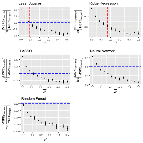
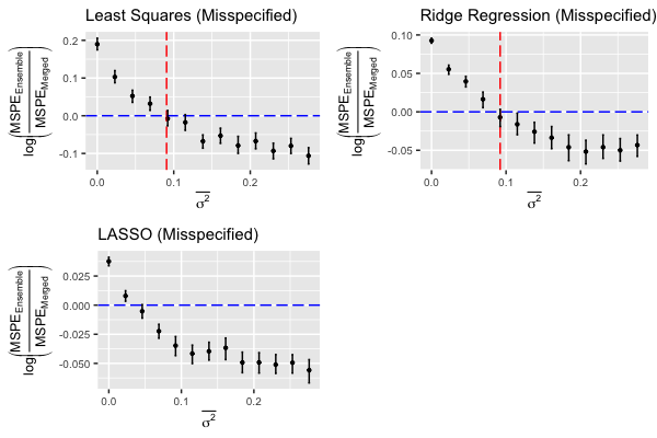
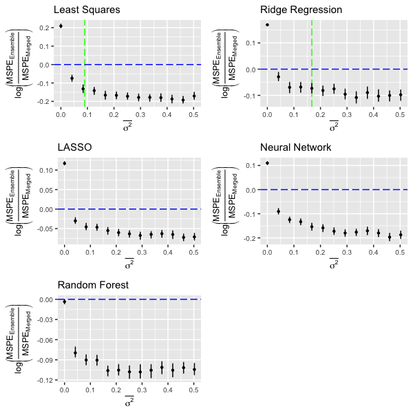
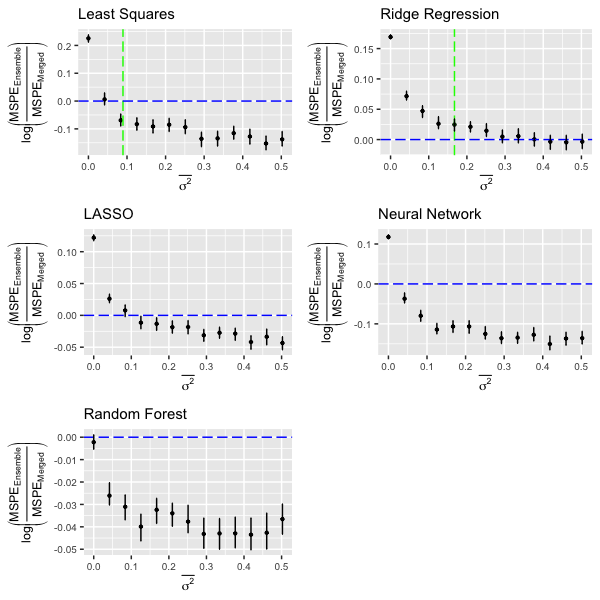
Our main simulation analysis was based on the setting of Theorem \arabicsection.\arabictheorem, where the random effects have equal variances . We considered choices of corresponding to different levels of heterogeneity ranging from to , where is the theoretical transition point for ridge regression from Theorem \arabicsection.\arabictheorem. We performed another analysis based on the setting of Theorem \arabicsection.\arabictheorem, where the random effects have unequal variances. For this analysis, we considered choices of corresponding to levels of heterogeneity ranging from to , where is the theoretical upper bound of the transition interval from Theorem \arabicsection.\arabictheorem. For each choice of and each study , including the test study =0, the outcomes were generated from using the following steps: 1) sample the random effects from , 2) sample the residual errors independently from with , and 3) generate using Model \arabicequation and the functional form given in Equation \arabicequation.
We trained and tested the following approaches: a correctly specified linear mixed effects model and merged and ensemble learners based on least squares, ridge regression, lasso, neural networks, and random forests. For least squares, ridge regression, and lasso, we considered fitting correctly specified models, i.e. using the correct basis expansion for the predictors, in the main analysis, but also conducted a sensitivity analysis with misspecified models. For ridge regression, lasso, random forest, and neural network, the following hyperparameters were chosen using 5-fold cross-validation in a tuning dataset of size 250 that was not used for training: the regularization parameter for ridge regression and lasso, the number of predictors sampled at each split for random forest, and the number of nodes and weight decay parameter for neural network. We restricted to neural networks with a single hidden layer to limit the computational burden. The outcomes in the tuning dataset were generated under .The hyperparameters for the merged versions of the models were selected using the entire tuning dataset while the hyperparameters for the study-specific models were selected using a subset of size 50.
In addition to the simulations with studies and diagonal , we performed sensitivity analyses considering scenarios with misspecified least squares/ridge regression/lasso models, i.e. using the original predictors without basis expansion, and instead of training studies, studies of size instead of , and scenarios with correlated random effects.
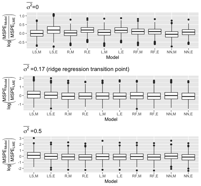
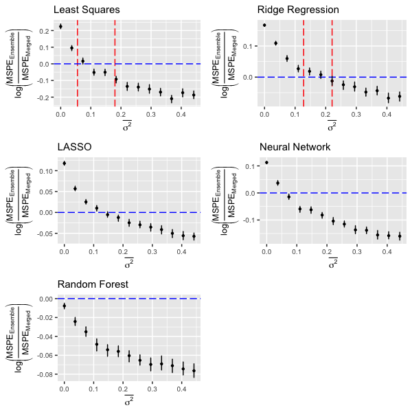
The results from the main simulation analysis based on Theorem \arabicsection.\arabictheorem are shown in Figure \arabicfigure and Figure A.\arabicfigure while the results from the other scenarios are provided in Figures A.\arabicfigure-A.\arabicfigure. The performance of the models relative to the data generating model in the main simulation analysis is summarized in Figure A.\arabicfigure for three values of . When , the merged regression learners perform as well as or slightly better than the generating model and outperform the ensembles. In particular, the merged neural network performs better than the generating model. At the ridge regression transition point, all models perform similarly. Beyond the transition point, the models continue to perform similarly, with the ensembles slightly outperforming the merged learners. In the scenarios with uncorrelated random effects, i.e. the scenarios for which we derived theoretical results (Figure \arabicfigure and Figures A.\arabicfigure-A.\arabicfigure), the empirical transition points for least squares and ridge regression agree with the theoretical results regardless of whether the models were correctly specified. Also, in each scenario, the transition points of the different methods did not vary substantially except that the random forest either had no transition point because ensembling always outperformed merging (Figure \arabicfigure and Figure A.\arabicfigure) or had a much earlier transition point than the other methods (Figures A.\arabicfigure-A.\arabicfigure). This may be related to the fact that a single random forest is already an ensemble of decision trees. In the scenarios with correlated random effects (Figures A.\arabicfigure and A.\arabicfigure), the least squares transition point occurred earlier than when the random effects were uncorrelated. In the positive correlation scenario, the ridge regression transition point also occurred earlier than when the random effects were uncorrelated, but the opposite was true in the negative correlation scenario.
\arabicsection Metagenomics Application
Growing research on associations between the gut microbiome and health-related outcomes has motivated the development of prediction models based on metagenomic sequencing data (Fu et al., 2015; Gupta et al., 2020). The ability to predict health status from microbiome samples can help guide the design of controlled intervention studies that target the microbiome, for example using diet or probiotics. In our data example, we focus on cholesterol, a strong risk factor for cardiovascular disease. Studies have shown that the microbiome is associated with blood cholesterol levels (Fu et al., 2015; Le Roy et al., 2019; Kenny et al., 2020). In particular, the metabolism of intestinal cholesterol by gut bacteria may reduce the amount of cholesterol absorbed from the intestine, resulting in lower blood cholesterol (Kenny et al., 2020). Recent work has identified bacterial genes involved in cholesterol metabolism (Kenny et al., 2020).
To illustrate in a practical example, we compared the performance of merging and ensembling in developing models to predict cholesterol levels from metagenomic sequencing data. We used datasets from the curatedMetagenomicData R package (Pasolli et al., 2017), which contains a collection of curated, uniformly processed whole-metagenome sequencing data from multiple studies. In addition to metagenomic data such as gene marker abundance, it also includes demographic and clinical data. Cholesterol measurements were available for three of the studies that sequenced gut microbial DNA: 1) a study of Chinese type 2 diabetes patients and non-diabetic controls, including female patients (Qin et al., 2012), 2) a study of middle-aged European women with normal, impaired or diabetic glucose control (Karlsson et al., 2013), and 3) a study of patients with a family history of type 1 diabetes (Heintz-Buschart et al., 2017). We used samples from female patients in these studies. The sample sizes were 151, 145, and 32 for the three studies.
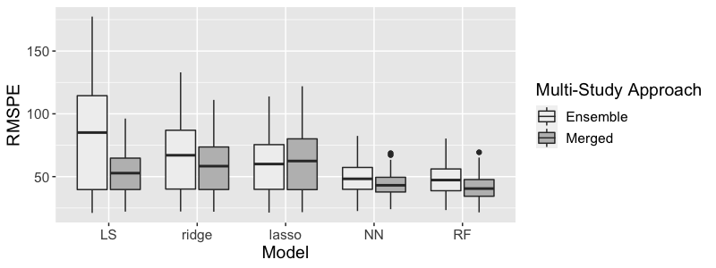
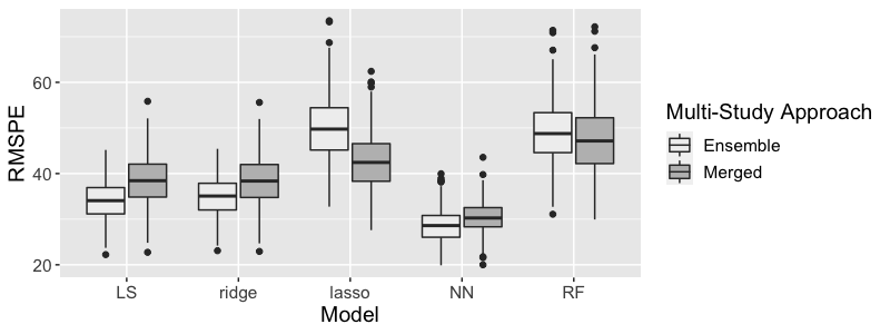
We used merging and ensembling to train least squares, ridge regression, lasso, neural network, and random forest models to predict cholesterol, calculated the theoretical transition intervals for least squares and ridge regression, and evaluated the performance of the approaches. We considered two scenarios: 1) training on different subsets of the same study and testing on a held out subset, and 2) training on different studies and testing on an independent study. In the first scenario, we randomly split the samples from Qin et al. (2012) into five datasets of approximately equal size, using for training and the remaining one for testing. In second scenario, we used the datasets from Qin et al. (2012) and Karlsson et al. (2013) for training and dataset from Heintz-Buschart et al. (2017) for testing. We used age and gene marker abundance for a selected set of gene markers as the predictors. Due to the limited sample sizes, we restricted to a small number of gene markers when fitting the prediction models. In the first scenario, we selected the top five gene markers that were most highly correlated with cholesterol in the training set and in the second scenario, we selected the top twenty gene markers that were most highly correlated with cholesterol in the training set. See Appendix C in the supplementary materials for a list of the selected gene markers. In each scenario, we fit merged and ensemble versions of least squares, ridge regression, lasso, neural network, and random forest. The linear models were specified as where contained 7 elements in the first scenario - intercept, age, and 5 gene markers - and 22 elements in the second scenario - intercept, age, and 20 gene markers. To estimate the transition intervals, we estimated by fitting a linear mixed effects model using residual maximum likelihood, allowing each predictor to have a random effect: We estimated the optimal weights for least squares and ridge regression using Proposition \arabicsection.\arabictheorem and estimates of , , and from the mixed effects model. We calculated the theoretical transition bounds from Theorem \arabicsection.\arabictheorem assuming a linear generating model and compared them to the estimate of . We used the optimal weights for ridge regression to ensemble the study-specific lasso, neural network, and random forest models. We evaluated the performance of merging and ensembling by calculating the prediction error on the test set.
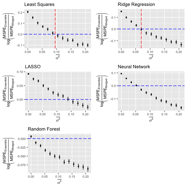
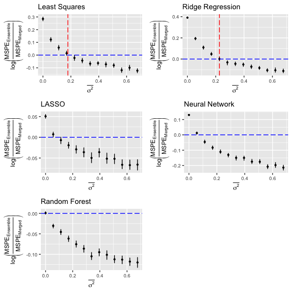
In the first scenario, was estimated to be , the lower bound of the transition interval for least squares was , and the lower bound of the transition interval for ridge regression was , so merging was expected outperform ensembling. In the test set, the merged versions of all of the models except lasso had lower prediction error than the corresponding ensembles (Figure \arabicfigure). In the second scenario, was estimated to be , the upper bound of the transition interval for least squares was , and the upper bound of the transition interval for ridge regression was , so ensembling was expected to outperform merging. In the test set, the ensemble versions of least squares, ridge regression, and neural network had lower prediction error than the corresponding merged learners, while merging outperformed ensembling for lasso and merging performed similarly to ensembling for random forest (Figure \arabicfigure). Lasso and random forest both had considerably higher prediction error than the other models.
\arabicsection Discussion
The availability of large though somewhat heterogeneous collections of data for training classifiers is challenging traditional approaches for training and validating prediction and classification algorithms. At the same time, it is creating opportunities for new and more general paradigms. One of these is multi-study ensemble learning, motivated by variation in the relation between predictors and outcomes across collections of similar studies. A natural benchmark for these methods is to combine all training studies to exploit the power of larger training sample sizes. In previous work (Patil & Parmigiani, 2018), merged learners were shown to perform better than ensemble learners in simulations under low-heterogeneity settings. As heterogeneity increased, however, there was a transition point in the heterogeneity scale beyond which acknowledging cross-study heterogeneity became preferable, and the ensemble learners outperformed the merged learners.
In this paper, we provide the first theoretical investigation of multi-study ensembling. Using a flexible data generating framework based on a nonparametric mixed effects model, we have been able to prove that when prediction is done using linear models, multi-study ensembling can, under certain conditions, achieve better optimality properties than merging all studies prior to training, a question that was still open. The class of linear models we have considered includes regularized and basis-expanded models, which are able to provide reasonable approximations of potentially nonlinear data generating models. We characterized the relative performance of merging and ensembling as a function of inter-study heterogeneity, explicitly identifying the transition point beyond which ensembling outperforms merging for least squares and ridge regression. These results are applicable to both correctly specified and misspecified linear prediction models. We confirmed the analytic results in simulations and demonstrated that when the data are generated by a mixed effects model, the least squares and ridge regression solutions can potentially serve as proxies for the transition point under other learning strategies (lasso, neural network) for which closed-form derivation is difficult. Finally, we estimated the transition point in cases of low and high cross-study heterogeneity in microbiome data and showed how it can be used as a guide for deciding when and when not to merge studies together in the course of learning a prediction rule.
We focused on deriving analytic results for ridge regression and its variants, including least squares and penalized spline regression, because of the opportunity to pursue closed-form solutions. Other widely used methods such as lasso, neural networks, and random forests are not as easily amenable to a closed-form solution, so we used simulations to investigate whether the analytic results we derived could potentially serve as an approximation for these methods. In our simulation settings, the empirical transition points of least squares, ridge regression, lasso, and neural networks fell within a similar range, but the random forests showed very different behavior. In one setting, the ensemble version of the random forest always outperformed the merged version and there was no transition point, while in other settings, the transition for the random forest occurred much earlier than for the other models. A key difference between random forests and the other methods considered is that a single random forest is already an ensemble of decision trees, which potentially complicates the comparison of merging to ensembling. Further exploration of this issue is provided by Ramchandran et al. (2020). The simulation results suggest that in some scenarios it may be reasonable to use the transition points for ridge regression or least squares as a proxy when considering machine learning models such as lasso or neural networks. However, the results are not generalizable to random forests and our data example shows that lasso can sometimes behave very differently from ridge regression and least squares, so caution is needed in using such approximations. Also, it is important to consider how the reliability of such approximations could be affected by the choice of model hyperparameters.
In practice, the analytic transition point and transition interval expressions could be used to help guide decisions about whether to merge data from multiple studies when there is potential heterogeneity in predictor-outcome relationships across the study populations. can be estimated from the training data and compared to the theoretical transition points or bounds for least squares and/or ridge regression. Various methods can be used to estimate , including maximum likelihood and method of moments-based approaches used in meta-analysis (for example, see Jackson et al. 2016), with the caveat that estimates will be imprecise when the number of studies is small.
Under Model \arabicequation, fitting a correctly specified mixed effects model will generally be more efficient than both the merged and ensemble versions of least squares. However, more flexible machine learning algorithms can potentially yield better prediction accuracy than the true model. For example, in the main simulation analysis, the mixed effects model was outperformed by a neural network. Moreover, fitting a mixed effects model can be computationally difficult when the number of predictors is large and standard mixed effects models are not appropriate for high-dimensional data, though there are methods for penalized mixed effects models (Bondell et al., 2010; Ibrahim et al., 2011; Schelldorfer et al., 2011; Fan & Li, 2012).
A limitation of our derivations is that they treat the following quantities as known: the subset of predictors with random effects, the ensemble weights, and the regularization parameters for ridge regression. In practice, these are usually selected using statistical procedures that introduce additional variability. Furthermore, we obtained closed-form transition point expressions for cases where the ensemble weighting scheme does not depend on the variances of the random effects. Such weighting schemes are generally sub-optimal, as the optimal weights given by Proposition \arabicsection.\arabictheorem depend on . Therefore, the closed-form results are based on a conservative estimate of the maximal performance of multi-study ensembling. Another limitation is the assumption that the random effects are uncorrelated, which is often not true in practice.
In summary, although this work is predicated upon the assumption that cross-study heterogeneity manifests as random effects and assumes that weights and regularization parameters are known, we believe it provides a theoretical rationale for multi-study ensembling and a strong foundation for developing practical rules and guidelines to implement it.
Acknowledgement
The authors thank Lorenzo Trippa and Boyu Ren for useful discussions. Work supported by NSF-DMS grant 1810829 and NSERC PGSD3 - 502362 - 2017.
Code
Code to reproduce the simulations and data application is available at
https://github.com/zoeguan/transition_point.
References
- Benito et al. (2004) Benito, M., Parker, J., Du, Q., Wu, J., Xiang, D., Perou, C. M. & Marron, J. S. (2004). Adjustment of systematic microarray data biases. Bioinformatics 20, 105–114.
- Bernau et al. (2014) Bernau, C., Riester, M., Boulesteix, A.-L., Parmigiani, G., Huttenhower, C., Waldron, L. & Trippa, L. (2014). Cross-study validation for the assessment of prediction algorithms. Bioinformatics 30, i105–i112. PMCID: PMC4058929.
- Bondell et al. (2010) Bondell, H. D., Krishna, A. & Ghosh, S. K. (2010). Joint variable selection for fixed and random effects in linear mixed-effects models. Biometrics 66, 1069–1077.
- Bravata & Olkin (2001) Bravata, D. M. & Olkin, I. (2001). Simple pooling versus combining in meta-analysis. Evaluation & the health professions 24, 218–230.
- Castaldi et al. (2011) Castaldi, P. J., Dahabreh, I. J. & Ioannidis, J. P. (2011). An empirical assessment of validation practices for molecular classifiers. Briefings in bioinformatics 12, 189–202.
- de Vlaming & Groenen (2015) de Vlaming, R. & Groenen, P. J. (2015). The current and future use of ridge regression for prediction in quantitative genetics. BioMed research international 2015.
- Dietterich (2000) Dietterich, T. G. (2000). Ensemble methods in machine learning. In International workshop on multiple classifier systems. Springer.
- Edgar et al. (2002) Edgar, R., Domrachev, M. & Lash, A. E. (2002). Gene expression omnibus: Ncbi gene expression and hybridization array data repository. Nucleic acids research 30, 207–210.
- Fan & Li (2012) Fan, Y. & Li, R. (2012). Variable selection in linear mixed effects models. Annals of statistics 40, 2043.
- Fu et al. (2015) Fu, J., Bonder, M. J., Cenit, M. C., Tigchelaar, E. F., Maatman, A., Dekens, J. A., Brandsma, E., Marczynska, J., Imhann, F., Weersma, R. K. et al. (2015). The gut microbiome contributes to a substantial proportion of the variation in blood lipids. Circulation research 117, 817–824.
- Gorgolewski et al. (2017) Gorgolewski, K., Esteban, O., Schaefer, G., Wandell, B. & Poldrack, R. (2017). Openneuro—a free online platform for sharing and analysis of neuroimaging data. Organization for Human Brain Mapping. Vancouver, Canada , 1677.
- Gu et al. (2005) Gu, C., Ma, P. et al. (2005). Optimal smoothing in nonparametric mixed-effect models. The Annals of Statistics 33, 1357–1379.
- Gupta et al. (2020) Gupta, V. K., Kim, M., Bakshi, U., Cunningham, K. Y., Davis, J. M., Lazaridis, K. N., Nelson, H., Chia, N. & Sung, J. (2020). A predictive index for health status using species-level gut microbiome profiling. Nature communications 11, 1–16.
- Hansen & Pedersen (2003) Hansen, F. & Pedersen, G. K. (2003). Jensen’s operator inequality. Bulletin of the London Mathematical Society 35, 553–564.
- Heintz-Buschart et al. (2017) Heintz-Buschart, A., May, P., Laczny, C. C., Lebrun, L. A., Bellora, C., Krishna, A., Wampach, L., Schneider, J. G., Hogan, A., de Beaufort, C. et al. (2017). Integrated multi-omics of the human gut microbiome in a case study of familial type 1 diabetes. Nature microbiology 2, 16180.
- Ibrahim et al. (2011) Ibrahim, J. G., Zhu, H., Garcia, R. I. & Guo, R. (2011). Fixed and random effects selection in mixed effects models. Biometrics 67, 495–503.
- Jackson et al. (2016) Jackson, D., Law, M., Barrett, J. K., Turner, R., Higgins, J. P., Salanti, G. & White, I. R. (2016). Extending dersimonian and laird’s methodology to perform network meta-analyses with random inconsistency effects. Statistics in medicine 35, 819–839.
- Jackson et al. (2011) Jackson, D., Riley, R. & White, I. R. (2011). Multivariate meta-analysis: potential and promise. Statistics in medicine 30, 2481–2498.
- Jackson et al. (2010) Jackson, D., White, I. R. & Thompson, S. G. (2010). Extending dersimonian and laird’s methodology to perform multivariate random effects meta-analyses. Statistics in medicine 29, 1282–1297.
- Jiang et al. (2004) Jiang, H., Deng, Y., Chen, H.-S., Tao, L., Sha, Q., Chen, J., Tsai, C.-J. & Zhang, S. (2004). Joint analysis of two microarray gene-expression data sets to select lung adenocarcinoma marker genes. BMC bioinformatics 5, 81.
- Karlsson et al. (2013) Karlsson, F. H., Tremaroli, V., Nookaew, I., Bergström, G., Behre, C. J., Fagerberg, B., Nielsen, J. & Bäckhed, F. (2013). Gut metagenome in european women with normal, impaired and diabetic glucose control. Nature 498, 99.
- Kenny et al. (2020) Kenny, D. J., Plichta, D. R., Shungin, D., Koppel, N., Hall, A. B., Fu, B., Vasan, R. S., Shaw, S. Y., Vlamakis, H., Balskus, E. P. et al. (2020). Cholesterol metabolism by uncultured human gut bacteria influences host cholesterol level. Cell host & microbe 28, 245–257.
- Kosch & Jung (2018) Kosch, R. & Jung, K. (2018). Conducting gene set tests in meta-analyses of transcriptome expression data. Research synthesis methods .
- Krogh & Vedelsby (1995) Krogh, A. & Vedelsby, J. (1995). Neural network ensembles, cross validation, and active learning. In Advances in neural information processing systems.
- Lagani et al. (2016) Lagani, V., Karozou, A. D., Gomez-Cabrero, D., Silberberg, G. & Tsamardinos, I. (2016). A comparative evaluation of data-merging and meta-analysis methods for reconstructing gene-gene interactions. BMC bioinformatics 17, S194.
- Lazar et al. (2012) Lazar, C., Meganck, S., Taminau, J., Steenhoff, D., Coletta, A., Molter, C., Weiss-Solís, D. Y., Duque, R., Bersini, H. & Nowé, A. (2012). Batch effect removal methods for microarray gene expression data integration: a survey. Briefings in bioinformatics 14, 469–490.
- Le Roy et al. (2019) Le Roy, T., Lécuyer, E., Chassaing, B., Rhimi, M., Lhomme, M., Boudebbouze, S., Ichou, F., Barceló, J. H., Huby, T., Guerin, M. et al. (2019). The intestinal microbiota regulates host cholesterol homeostasis. BMC biology 17, 1–18.
- Parkinson et al. (2010) Parkinson, H., Sarkans, U., Kolesnikov, N., Abeygunawardena, N., Burdett, T., Dylag, M., Emam, I., Farne, A., Hastings, E., Holloway, E. et al. (2010). Arrayexpress update—an archive of microarray and high-throughput sequencing-based functional genomics experiments. Nucleic acids research 39, D1002–D1004.
- Pasolli et al. (2017) Pasolli, E., Schiffer, L., Manghi, P., Renson, A., Obenchain, V., Truong, D. T., Beghini, F., Malik, F., Ramos, M., Dowd, J. B. et al. (2017). Accessible, curated metagenomic data through experimenthub. Nature methods 14, 1023.
- Patil & Parmigiani (2018) Patil, P. & Parmigiani, G. (2018). Training replicable predictors in multiple studies. Proceedings of the National Academy of Sciences 115, 2578–2583.
- Qin et al. (2012) Qin, J., Li, Y., Cai, Z., Li, S., Zhu, J., Zhang, F., Liang, S., Zhang, W., Guan, Y., Shen, D. et al. (2012). A metagenome-wide association study of gut microbiota in type 2 diabetes. Nature 490, 55.
- Ramchandran et al. (2020) Ramchandran, M., Patil, P. & Parmigiani, G. (2020). Tree-weighting for multi-study ensemble learners. Pacific Symposium on Biocomputing , 451–462.
- Rashid et al. (2019) Rashid, N. U., Li, Q., Yeh, J. J. & Ibrahim, J. G. (2019). Modeling between-study heterogeneity for improved replicability in gene signature selection and clinical prediction. Journal of the American Statistical Association 0, 1–14.
- Riester et al. (2012) Riester, M., Taylor, J. M., Feifer, A., Koppie, T., Rosenberg, J. E., Downey, R. J., Bochner, B. H. & Michor, F. (2012). Combination of a novel gene expression signature with a clinical nomogram improves the prediction of survival in high-risk bladder cancer. Clinical Cancer Research 18, 1323–1333.
- Schelldorfer et al. (2011) Schelldorfer, J., Bühlmann, P. & DE GEER, S. V. (2011). Estimation for high-dimensional linear mixed-effects models using l1-penalization. Scandinavian Journal of Statistics 38, 197–214.
- Stone (1948) Stone, M. H. (1948). The generalized weierstrass approximation theorem. Mathematics Magazine 21, 237–254.
- Taminau et al. (2014) Taminau, J., Lazar, C., Meganck, S. & Nowé, A. (2014). Comparison of merging and meta-analysis as alternative approaches for integrative gene expression analysis. ISRN bioinformatics 2014.
- Tseng et al. (2012) Tseng, G. C., Ghosh, D. & Feingold, E. (2012). Comprehensive literature review and statistical considerations for microarray meta-analysis. Nucleic acids research 40, 3785–3799.
- Tsybakov (2014) Tsybakov, A. B. (2014). Aggregation and minimax optimality in high-dimensional estimation.
- Wang (1998) Wang, Y. (1998). Mixed effects smoothing spline analysis of variance. Journal of the royal statistical society: Series b (statistical methodology) 60, 159–174.
- Xu et al. (2008) Xu, L., Tan, A. C., Winslow, R. L. & Geman, D. (2008). Merging microarray data from separate breast cancer studies provides a robust prognostic test. BMC bioinformatics 9, 125.
- Zhang et al. (2018) Zhang, Y., Bernau, C., Parmigiani, G. & Waldron, L. (2018). The impact of different sources of heterogeneity on loss of accuracy from genomic prediction models. Biostatistics , kxy044.
- Zhou et al. (2017) Zhou, H. H., Zhang, Y., Ithapu, V. K., Johnson, S. C., Wahba, G. & Singh, V. (2017). When can multi-site datasets be pooled for regression? hypothesis tests, -consistency and neuroscience applications. arXiv preprint arXiv:1709.00640 .
Appendix A: Calculations and Proofs
.\arabicsubsection Covariance Matrices and MSPEs
The covariances and expectations are all conditional on the predictors.
.\arabicsubsection Proof of Theorem 2
Theorems 1 is a special case of Theorem 2.
Let .
Let .
Since
| (\arabicequation) |
and
| (\arabicequation) |
it follows that
Similarly,
.\arabicsubsection Optimal Weights
Ridge Regression. For ridge regression, let
We want to minimize
subject to the constraint .
Using Lagrange multipliers, we get the system of equations
| (for ) | ||||
The solution to the system is
| (\arabicequation) |
where the entries of are and for and .
| (\arabicequation) |
Least Squares Under a Linear Generating Model. For least squares, we want to minimize
subject to the constraint .
Using Lagrange multipliers, we get the system of equations
| (for ; is the Lagrange multiplier) | |||
which is solved by
Plugging the optimal weights into the MSPE of the ensemble learner, , we get
In the equal variances setting,
so is approximately linear in when is similar across studies or when is large.
Appendix B: Additional Plots
Appendix C: Gene Markers Used in Data Example
The gene markers selected for the first scenario in the data example were:
-
•
gi.512436192.ref.NZ_KE159480.1..202016.203626
-
•
gi.512436192.ref.NZ_KE159480.1..c204954.204127
-
•
gi.512436192.ref.NZ_KE159480.1..213329.214486
-
•
gi.512436192.ref.NZ_KE159480.1..c198594.196087
-
•
gi.512436192.ref.NZ_KE159480.1..c204130.203732
The gene markers selected for the second scenario were:
-
•
gi.479140210.ref.NC_021010.1..1710650.1711408
-
•
gi.238922432.ref.NC_012781.1..1198506.1198766
-
•
gi.238922432.ref.NC_012781.1..1209760.1211007
-
•
gi.479213596.ref.NC_021044.1..c2622668.2622303
-
•
gi.238922432.ref.NC_012781.1..c2899618.289912
-
•
gi.479140210.ref.NC_021010.1..3168417.3168521
-
•
gi.238922432.ref.NC_012781.1..c2301152.2300781
-
•
gi.238922432.ref.NC_012781.1..1311347.1311667
-
•
gi.238922432.ref.NC_012781.1..c753467.753039
-
•
gi.238922432.ref.NC_012781.1..c1926223.1925561
-
•
gi.238922432.ref.NC_012781.1..c2743334.2742522
-
•
gi.479213596.ref.NC_021044.1..1253015.1253476
-
•
gi.479213596.ref.NC_021044.1..c2217719.2217459
-
•
gi.479208076.ref.NC_021042.1..c657163.656546
-
•
gi.545411814.ref.NZ_KE993320.1..c60369.59749
-
•
gi.211596842.ref.NZ_DS264296.1..41162.41911
-
•
gi.479140210.ref.NC_021010.1..2564135.2565262
-
•
gi.238922432.ref.NC_012781.1..c2485168.2484434
-
•
gi.224485442.ref.NZ_EQ973177.1..c62806.61865
-
•
gi.479213596.ref.NC_021044.1..c2624541.2623825
Appendix D: Notation Table
| Variable | Value / Description |
|---|---|
| number of training studies | |
| sample size in study ( corresponds to test dataset) | |
| outcome for individual in study | |
| outcome vector for study | |
| th predictor for individual in study | |
| vector of predictors for individual in study | |
| fixed effects design matrix for study | |
| ; design matrix for merged dataset | |
| basis-expanded version of used to fit ridge regression prediction models | |
| basis-expanded version of used to fit ridge regression prediction models | |
| ; outcome vector for merged dataset | |
| number of original predictors (including the intercept if applicable) | |
| number of predictors with random effects | |
| true function relating to such that | |
| true function relating to such that ; | |
| vector of random effects | |
| variance of random effect | |
| ; covariance matrix for random effects | |
| ; heterogeneity summary measure | |
| number of unique variance values for random effects | |
| distinct values on the diagonal of | |
| number of random effects with variance | |
| vector of residual errors for study | |
| variance of residuals | |
| ensemble weight for study | |
| basis-expanded design matrix for study | |
| basis function | |
| basis-expanded design matrix ridge design matrix for merged dataset | |
| if an intercept is included in the ridge regression model and otherwise | |
| ; ridge regression estimator from study | |
| ; ensemble ridge regression estimator | |
| ; merged ridge regression estimator | |
| transition point for ridge regression (Theorem 1) | |
| lower bound of transition interval for ridge regression (Theorem 2) | |
| upper bound of transition interval for ridge regression (Theorem 2) | |