Temporal changes of the flare activity of Proxima Cen

Abstract

Context. We study temporal variations of the emission lines of $H_{\alpha}$, H_ϵ, H and K CaI, D₁ and D₂ NaI, He₄₀₂₆, and He₅₈₇₆ in the HARPS spectra of Proxima Centauri across an extended time of 13.2 years, from May 27, 2004, to September 30, 2017.

Aims. We analyse the common behaviour and differences in the intensities and profiles of different emission lines in flare and quiet modes of Proxima activity.

Methods. We compare the pseudo-equivalent widths ($pEW$) and profiles of the emission lines in the HARPS high-resolution (R $\sim$ 115,000) spectra observed at the same epochs.

Results. All emission lines show variability with a timescale of at least 10 min. The strength of all lines except He₄₀₂₆ correlate with $H_{\alpha}$. During strong flares the ‘red asymmetry’ appears in the $H_{\alpha}$ emission line indicating the infall of hot condensed matter into the chromosphere with velocities greater than 100 km/s disturbing chromospheric layers. As a result, the strength of the Ca II lines anti-correlates with $H_{\alpha}$ during strong flares. The HeI lines at 4026 and 5876 Å appear in the strong flares. The cores of D₁ and D₂ NaI lines are also seen in emission. During the minimum activity of Proxima Centauri, CaII lines and H_ϵ almost disappear while the blue part of the NaI emission lines is affected by the absorption in the extending and condensing flows.

Conclusions. We see different behaviour of emission lines formed in the flare regions and chromosphere. Chromosphere layers of Proxima Cen are likely heated by the flare events; these layers are cooled in the ‘non-flare’ mode. The self-absorption structures in cores of our emission lines vary with time due to the presence of a complicated system of inward and outward matter flows in the absorbing layers.

1 Introduction

In this paper we define ‘flare activity’ as a strong and time-variable phenomenon observed in stellar spectra and caused by the dissipation of magnetic field originated by dynamo processes in the stellar photosphere, in the chromosphere, or in the corona (e.g. Parker 1955). These processes differ comparatively from the case of slow phenomena of ‘stellar activity’ responsible for variations of observed fluxes due to comparatively slow variations of spots and filament structures on the stellar surface. Observationally, the dynamo mechanism can be probed through the relationship between rotation and magnetic activity, and the evolution of these properties (Suárez Mascareño et al. 2015; Newton et al. 2017).

Magnetic activity in late-type stars is often measured in terms of $H_{\alpha}$ emission and increases with decreasing stellar mass (e.g. Hawley et al. 1996). Magnetic activity increases with decreasing stellar mass; for example, Hawley et al. (1996). In addition, magnetically active stars are known to flare more frequently than inactive stars. Magnetic activity, stellar rotation and magnetic field strength configuration are intrinsically linked. We believe that stellar flares are caused by the reconnection of surface magnetic field loops (see, e.g. Yokoyama & Shibata (1998) and reference therein). The correlation between magnetic field in active regions is very clear in the case of solar flares (Fletcher et al. 2011) meaning that stellar flares may be used as a proxy for magnetic activity.

The fraction of stars showing $H_{\alpha}$ in their emission (Delfosse et al. 1998) or frequent flares (Hawley & Pettersen 1991; Schmidt et al. 2014; Hawley et al. 2014) increases with decreasing mass, mainly due to their longer rotational braking times (Delfosse et al. 1998; Barnes 2003; Delorme et al. 2011). The braking rates strongly depend on the spectral type (or mass) of the star (Barnes 2003; Barnes & Kim 2010), which results in partially convective low-mass stars spinning down slower than their higher-mass counterparts. Fully convective stars have even longer rotational braking timescales (Reiners & Basri 2008; Browning et al. 2010). Low-mass M dwarfs exhibit stronger chromospheric and coronae emissions for a given rotation period than more massive G–K dwarfs (see fig. 6 in Kiraga & Stepien 2007a). On the other hand, rotation and magnetic activity of stars decrease with time as a consequence of magnetic braking, that is the angular momentum is extracted from the convective envelope and lost through a magnetized wind (Skumanich 1972; Mestel 1984; Mestel & Spruit 1987).

M dwarfs make up 70% of the stars in the solar neighbourhood. They are small, cool main sequence stars with temperatures in the range 2400–3800 K and radii between 0.10 and 0.63 R$\odot$. Radii of M dwarfs are smaller than solar-like stars, implying that the flare activity phenomena are more pronounced at the background of their cool photospheres. M dwarfs with spectral types later than M4 have fully convective atmospheres with no boundary zone between the radiative and convective zones (Hawley et al. 2014), implying that we do not expect significant magnetic fields such as those generated in the Sun (Doyle et al. 2018). The magnetic fields present at the surface of low-mass M dwarfs (M5–M8) originate either from strong, axisymmetric dipole fields or from weak, higher-order multipole fields (Morin et al. 2010, 2008).

Some of the first detailed optical observations of stellar flares on M dwarfs were reported by Bopp et al. (1973) and Gershberg & Shakhovskaia (1983); see also Gershberg (2005). X-ray observations with the EXOSAT satellite detected the first flare in M dwarfs in the atmosphere of YZ CMi (Heise et al. 1975). Since then, the physics of stellar flares has been studied by different teams over a wide range of energy, from $\gamma$-ray to radio frequencies. The characterization of M dwarf flares has become possible thanks to the advent of large-scale surveys such as the Sloan Digital Sky Survey (SDSS; York et al. 2000). Kowalski et al. (2009) identified flares in the SDSS Stripe 82, where the authors found that active ($H_{\alpha}$ in emission) M dwarfs flared at approximately 30 times the rate of inactive M dwarfs. They also found that the flaring fraction increases for cooler stars, which they attribute in part to a higher fraction of magnetically active stars among late-M dwarfs. This is compatible with lower-mass stars rotating more rapidly over a long time-span (and therefore magnetically active) than their more massive counterparts. The presence of higher rates of flares in late-type M dwarfs impacts the exoplanet community because flares release large amounts of energy in the UV, which could potentially affect the atmospheres and habitability of orbiting exoplanets.

Recent large-scale radial velocity (RV) searches for extra-solar planets (Jenkins et al. 2017, and references therein) provide a new framework and motivation to study stellar and flare activity phenomena. Indeed, they provide extensive time series of high-resolution spectra obtained by the best spectrographs on the biggest telescopes for large samples of stars. The study of activity in exoplanet science is of special interest because spots, plages, and other inhomogeneities of the stellar surface affect the shape of spectral lines, shift their centroids, and consequently bias the measured RV (e.g. Barnes et al. 2011, and reference therein). Stellar and flare activity produce additional signals usually handled as random noise (the so-called RV jitter), which should be added to other known systematics such as photon noise and instrumental instabilities (Astudillo-Defru et al. 2015; Suárez Mascareño et al. 2017).

Today, M dwarfs represent important targets for searches of exoplanets. Due to their low mass and luminosity, M dwarfs are ideal targets to find low-mass, Earth-size planets with the RV technique (see Gomes da Silva et al. 2012, and references therein) and look for possible transits. The first rocky planets around M dwarfs were detected by RV and transits (Rivera et al. 2015; Charbonneau et al. 2009). We note that the first rocky planet Corot-7b orbiting a G9V star was announced by the COROT team (Léger et al. 2009; Queloz et al. 2009).

Proxima Cen was recently highlighted as a planet-host mid-M dwarf (Anglada-Escudé et al. 2016). Proxima Cen b orbits its host star with a period of 11.2 days, corresponding to a semi-major axis distance of 0.05 AU, and has a mass close to that of the Earth (from 1.10 to 1.46 Earth masses) and orbits in the temperate zone (Anglada-Escudé et al. 2016).

Proxima Cen is a known flare star that exhibits random but significant increases in brightness due to magnetic activity (Christian et al. 2004). The spectrum of Proxima Cen contains numerous emission lines (Fuhrmeister et al. 2011; Pavlenko et al. 2017). These features most likely originate from plages, spots, or a combination of both. Pavlenko et al. (2017) found the presence of hot evaporated matter flow originating from the outer envelope. The atmosphere of Proxima Cen shows a rather complicated structure consisting of the cool photosphere, chromosphere, and hot outer layers where even lines of HeI form. In general, the flare rate of Proxima Cen is lower than that of other flare stars of similar spectral type, but is unusually high given its slow rotation period (Davenport et al. 2016). The star has an estimated rotation period of $\sim$83 days and a magnetic cycle of about 7 years (Benedict et al. 1998; Suárez Mascareño et al. 2016; Wargelin et al. 2017). The X-ray coronal and chromospheric activity have been studied in detail by Fuhrmeister et al. (2011) and Wargelin et al. (2017). Recently, Thompson et al. (2017) claimed a detection of rotational modulation of emission lines in the spectrum of Proxima Cen.

West et al. (2015) suggested that the activity-rotation relation for the slow rotating stars may be more complicated than predicted by a simple spin-down model. One possibility could be that while persistent magnetic activity in late-type M dwarfs is rare (or non-existent) for slow rotators, the presence of magnetic cycles may produce observed activity in a small number of stars at any given time. As stated by Newton et al. (2016), many slowly rotating mid-to-late M dwarfs show variability amplitudes of half a per cent or more, implying that they have maintained strong-enough magnetic fields to produce the requisite spot contrasts. The lack of correlation between rotation period and amplitude for these stars indicates that the spot contrast is not changing significantly, even when they undergo substantial spin-down.

To date, most of the rocky planets in the habitable zone have been found around these very low-mass stars (Udry et al. 2007; Bonfils et al. 2011; Quintana & Barclay 2014; Torres et al. 2015; Wright et al. 2016; Anglada-Escudé et al. 2016). However, the flare activity of the hosting stars may affect the structure and temperature regime of the exoplanetary atmospheres, thereby affecting the size of the habitable zone. In March 2016, the Evryscope observed the first superflare visible to the naked eye detected from Proxima Cen (Howard et al. 2018). The brightness of Proxima Cen increased by a factor of 68 during this superflare and released a bolometric energy of 10^33.5 erg, i.e. approximately ten times larger than any flare detected before. Modelling photochemical effects of NOx atmospheric species generated by the severe particle events in the atmosphere of Proxima Cen b shows that the high level of the similar extreme strong flare activity in the long term is sufficient to reduce the ozone of an Earth-like atmosphere by 90% within five years. In other words, a conception of habitable zone should be reconsidered taking into account the impact of flare activity on exoplanet atmospheres (Howard et al. 2018).

In this paper, we focus on the temporal changes of emission lines in the optical spectra of Proxima Cen. We describe the observations in Sect. 2. We detail our procedure in Sect. 3. Section 4 presents our results, which we discuss and put into context in Sect. 5.

2 Optical spectra of Proxima obtained with 3.6-m/HARPS

We analysed 386 optical spectra obtained with HARPS, a fibre-fed, echelle, high-resolution spectrograph installed on the 3.6-m European Southern Observatory (ESO) telescope in the La Silla Observatory, Chile. The instrument offers a resolving power of R$\sim$115,000 over a spectral range from 3780 to 6810Å. The dates cover a time interval of over 13 years, from Barycentric Julian dates (BJD) between [245]3152.600, that is the night of May 27, 2004, and [245]6418.643, the night of September 30, 2017. In the remainder of the paper, we omit the prefix [245]. Most observations include one or two exposures per night, with some extended sets of exposures taken every $\sim$10 min at dates BJD = 6417 (May 4, 2013; number of exposures on that night is N_t = 55), 6418 (May 5, 2013; N_t = 64), 6420 (May 7, 2013; N_t = 22), and 6426 (May 13, 2013; N_t = 9). The HARPS observations cover an extended time interval providing a unique set of data to analyse the behaviour of stellar flares with time over a long period.

3 Procedure

We discuss the temporal changes of a few emission lines listed in Table 1. These lines result from different excitation potentials. Their formation requires different physical conditions, which occur in distant parts of the active atmosphere of Proxima Cen. Changes in the $pEW$ and line profiles of these emission lines reflect the direct or indirect impact of the flare activity on the whole stellar atmosphere, as well as their changes in time.

Table 1: Emission lines studied in our paper.

Line	$\lambda_{air}$ (Å)	Transition	$E_{l}$ (eV)	Formation regions
$H_{\alpha}$	6562.81	2P0 - 3S,D	10.199	Flares, facules
CaII (K)	3933.66	42S1/2 - 42P${}^{0}_{1/2}$)	0.0	Chromosphere
CaII (H)	3968.47	42S1/2 - 42P${}^{0}_{3/2}$	0.0	Chromosphere
He5876	5875.64	23P0-33D	20.964	Flares, transition zone
He4026	4026.19	23P0-53D	20.964	Flares, transition zone
Hϵ	3970.72	2P0 - 7S,D	10.199	Flares
NaI (D1)	5889.95	32S1/2 -32P${}^{0}_{3/2}$	0.0	Chromospheres
NaI (D2)	5895/92	32S1/2 -32P${}^{0}_{3/2}$	0.0	Chromospheres

We re-normalised the final 1D observed spectra to get the same flux in the background of these emission lines. This allows us to investigate the relative changes of $pEW$ of emission lines with time. As shown in Pavlenko et al. (2017), the changes of the background of emission lines appear rather marginal. In other words, activity processes do not affect photospheric levels, where the most absorption features and continuum form.

We measured $pEW$ of all emission lines listed in Table 1. Here we note that all these emission lines in the spectrum of Proxima Cen were analysed on the same spectra and, thus, at the same times. To investigate the temporal correlation between different emission lines formed in the flare events, we computed the Pearson $k_{p}$ and Stockman $k_{s}$ rank correlation coefficients to evaluate the changes in $pEW$ of our emission lines versus $H_{\alpha}$:

$${\displaystyle k_{p}={\frac{n\sum x_{i}y_{i}-\sum x_{i}\sum y_{i}}{{\sqrt{n\sum x_{i}^{2}-(\sum x_{i})^{2}}}\leavevmode\nobreak\ {\sqrt{n\sum y_{i}^{2}-(\sum y_{i})^{2}}}}},}$$

$$\begin{aligned} k_{s}={\frac{\sum(R(x_{i})-(n+1)/2)\times(R(y_{i})-(n+1)/2)}{(\sum(R(x_{i})-(n+1)/2))^{2}\times\sum(R(y_{i})-(n+1)/2))^{2})^{0.5}}}\end{aligned}.$$ (1)

These coefficients change in the range $-$1 $\leq$ $r_{xy}$ $\leq$ 1. By definition, the cases $k_{p}$, $k_{s}$ = 1, 0, $-$1 correspond to the strong correlation, no correlation, and strong anti-correlation, respectively.

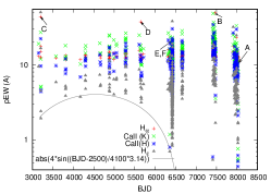
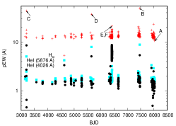
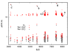
Figure 1: Variations of $pEW$ of emission lines at all dates of observations. The letter ‘A’ marks the absolute minimum of the $pEW$ of $H_{\alpha}$ (Section 4.4), letters ‘B’, ‘C’ and ‘D’ label the flares occasionally observed at BJD = 7465.8823, 3202.5647, and 5647.7300, respectively (Sect. 4.4) and letters ‘E’ and ‘F’ label the $pEW$ of two $H_{\alpha}$ flares observed across BJD = 6417 (Sect. 4.2). Grey line shows the approximation of the set of minimum values of $pEW$of H_ϵby a sinusoid; see Sect. 4.1.

4 Results

The variability of the $pEW$ of the selected emission lines on different dates is depicted in Fig. 1. These $pEW$ were determined for one dataset of the observed spectra. We draw our attention to a few expositions marked with the letters A, B, C, D, E, and F:

• The time mark ‘A’ locates the minimum level of activity of Proxima Cen, determined by the lowest $pEW$ of $H_{\alpha}$ (Sect. 4.4).

• The letters B, C, and D mark three flare events during observations on BJD = 6417 and 6418 (Sect. 4.5).

• The letters F and E mark two peaks of the ‘strong’ flare seen in $H_{\alpha}$ at BJD = 6414 (Sect. 4.8).

4.1 Long-term variatons of min H_ϵ

The temporal changes of the strength of the H_ϵ line provide some evidence about the presence of long-term variability in Proxima Cen. The emission in H_ϵ is weaker in comparison with $H_{\alpha}$, still its relative intensity is more sensitive to the level of activity in comparison with other lines. We derive a quasi-periodic variability of $\sim$ 8200 days by approximating the minimum values of the observed $pEW$ of H_ϵ at the dates BJD  = 3000–8000 by the relation $4*sin(2*\pi*(BJD-2500)/8200)$.

4.2 Temporal changes of the emission lines

We draw our attention to the temporal variability of emission lines in the spectrum of Proxima Cen. We argue that if all lines are formed in a single flare region of high temperature, we should see a strong correlation in their behaviours.

For simplicity, we adopt that the level of activity of Proxima Cen corresponds to the $pEW$ of $H_{\alpha}$ measured at a given date, that is, the minimum activity level of Proxima Cen corresponds to the minimum of the $pEW$ of $H_{\alpha}$ and vice versa. Indeed, the formation of $H_{\alpha}$ seen in emission is possible only in high-temperature regions heated by the flare events.

To analyse the relative temporal behaviour of $H_{\alpha}$ and other lines we computed the Pearson and Stockman correlation coefficients for each $pEW$ (Table 3). We note that the spectra observed between BJD = 6417 and 6429 were obtained with the Fabry-Perot wavelength calibration which generates some flux distortion at the exact position of the HeI at 4206 Å. Therefore, we excluded this line from our analysis for those dates.

In Table 3, we show the result of computations of the Pearson and Stockman correlation coefficients of the emission line strength with $H_{\alpha}$ for different time intervals. This was carried out (1) for all dates covered our interval of observations, from 3152.6001 to 6418.6431, except for BJD  =  6417 and 6429 in the case of the He₄₀₂₆ line, and (2) for two extended continuous sub-sets of observations of our lines except He₄₀₂₆ on BJD = 6417 and 6418 (Sect. 4.8).

In all cases we derive high positive values for the two correlation coefficients. In other words, we see that flare processes modulate the strength of all lines. Indeed, all lines follow the changes in intensity of $H_{\alpha}$. The He₄₀₂₆ line shows the weakest correlation with $H_{\alpha}$. We interpret this correlation as evidence that all lines are formed in or are affected by the same flare events which covered the broad range of heights in the stellar atmosphere.

In Fig. 11, we show the response of other lines on changes in the $pEW$ of $H_{\alpha}$. In fact, we can see three groups of lines with different correlation with $H_{\alpha}$, which can be roughly characterised by the gradient $b\,=\,d$($pEW$)/$d$($pEW$($H_{\alpha}$)). CaII H, K, and H_ϵ show larger $b$, while both helium lines show the weakest dependence; the relative response of NaI is stronger than He₄₀₂₆, but weaker than CaII H and K.

For convenience we implement a rather phenomenological classification of the strength of flares using quantitative criteria based on the values of the $pEW$ of H_ϵ (Table 2; Fig. 11).

Table 2: Classification of the strength of flares adopted in this paper

Classification	$pEW$(Hϵ)
0ϵ	0 $pEW$(Hϵ) $<$ 2 Å
1ϵ	2 $<$ $pEW$(Hϵ) $<$ 4 Å
2ϵ	4 $<$ $pEW$(Hϵ) $<$ 16 Å
3ϵ	$pEW$(Hϵ) $>$ 16 Å

We favour the use of H_ϵ to classify flares because its $pEW$ is strongly sensitive to the strength of flares. At the minimum of the flare activity, this line almost disappears (see Sect. 4.4). At maximum activity, the $pEW$ of H_ϵ might even be higher than the $pEW$($H_{\alpha}$), see Fig. 11. However, this is only true for $pEW$ computed with respect to the local pseudo-continuum, which can itself change during the flares (Sect. 4.6). Nonetheless, the equivalent widths of $H_{\alpha}$ always exceed the equivalent widths of H_ϵ due to the exponential drop of the flux towards the blue part of the spectrum.

Table 3: Pearson and Stockman correlation coefficients of the computed $pEW$ of the emission lines considered in this work vs. the $pEW$ of $H_{\alpha}$. Dates between BJD = 6417 and 6429 were not accounted for He₄₀₂₆ line (see Sect. 4.2).

	all, N=386		6417d, N=55		6418d, N=23
$H_{\alpha}$ vs. line	$k_{p}$	$k_{s}$	$k_{p}$	$k_{s}$	$k_{p}$	$k_{s}$
CaII (K)	0.8045	0.7229	0.9531	0.7832	0.8042	0.7955
CaII (H)	0.8897	0.7847	0.9753	0.8188	0.8068	0.8098
He5876	0.9288	0.8389	0.9377	0.7286	0.6407	0.6055
He4026	0.5265	0.4420
Hϵ	0.9068	0.7506	0.9210	0.8353	0.5907	0.6118
NaI(D2)	0.9397	0.8824	0.9456	0.7877	0.9673	0.9555
NaI(D1)	0.9496	0.8832	0.9489	0.8108	0.9628	0.9617

^∗ computed without dates between BJD = 6417 and 6429.

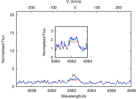
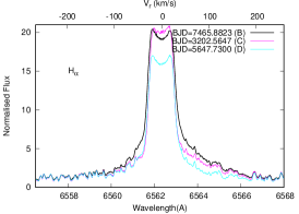
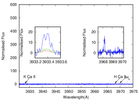
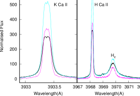
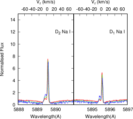
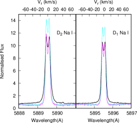
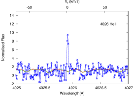
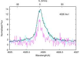
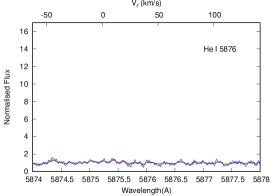
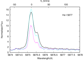
Figure 2: Left panel: Profiles of several emission lines, including $H_{\alpha}$, CaII K and H, NaI D₂ and D₁, He₅₈₇₆, and He₄₀₂₆ at the three dates of minimum activity of Proxima Cen: BJD = 8021.4600 (red), 8023.4639 (green), and 8027.4785 (blue). These dates are marked with letter ‘A’ in Fig. 1. Right panel: ‘Same lines at the dates of maximum of activity of Proxima Cen, i.e. BDJ = 7465.8823 (B; black), 3202.5647 (C; cyan), 5647.7300 (D; magenta) displayed in Fig. 1

.

4.3 Photosphere, chromosphere, and flare regions

In this paper, we discuss different aspects of the flare activity of Proxima Cen. For simplicity, we adopt that the atmosphere of Proxima Cen consists of three parts:

– The photosphere is the deepest part of the atmosphere, in which molecular and atomic absorption spectrum of Proxima. The photosphere of Proxima seems to be stable; flares do not affect its structure, because molecular lines are practically not affected by the flare events.

– The chromosphere lies above the photosphere and the temperature increases outwards. Here the formation of most emission lines occurs in NLTE. The chromosphere is a quasi-stable structure heated by the dissipation of non-thermal flows from the convective photosphere. Chromospheric lines are comparatively narrow due to absence of large-scale moves.

– According to modern notions, the flares are located in the outer part of a chromosphere and/or in the corona. Again, for simplicity we adopt flare conception described in Yokoyama & Shibata (1998). Just after an avalanche-like process of the release of energy due to the re-connection of magnetic field loops a small volume of the atmosphere of Proxima Cen (up to a few percent of the surface in the case of strongest flares) is heated up to 10⁶ K or more. Afterwards, the upward flows of hot matter from chromosphere (evaporation) and downward flows of cooling matter (condensation) toward photosphere are formed. Due to the higher temperatures in the flare regions, thermal and non-thermal motions are much higher and emission lines are broader than chromospheric lines. We follow this simplified model to avoid the uncertainty of interpretation of our observed data due to different conceptions based on the numerous theoretical models. In reality, a flare is a multi-dimensional magnetohydrodynamic process, which is variable on short timescales. Current models of flares are much more complicated (Zhang et al. 2016, and references therein); the analysis of which is beyond the scope of this paper.

4.4 Emission lines at the minimum activity of Proxima Cen

The photospheric spectrum at least in the optical and near-infrared spectral region shows rather marginal response to the flares (Pavlenko et al. 2017). On the contrary, both profiles and intensities of our emission lines respond to the changes of activity; see Fig. 1.

Firstly, we find the three lowest $pEW$ of $H_{\alpha}$ in the spectrum of Proxima Cen, with $pEW$ of 10.62Å, 11.34Å, and 11.39Å at dates BJD = 8021.4600, 8023.4639, and 8027.4785, respectively. The exposure taken on BJD = 8021.4600 is marked by ‘A’ in Fig. 1. These three dates differ by only a few days and show a minimum activity level of Proxima Cen.

The left-hand side panel of Fig. 2 compares the level of activity of the selected lines on those three dates of minimum activity of Proxima Cen. The right-hand side panel of Fig. 2 shows the relative change of these lines between the times of maximum and minimum activity.

At times of minimum activity, we find the following.

• We still see an emission component in the blue wing of $H_{\alpha}$ with $V$ = $-$30 km/s (Pavlenko et al. 2017), formed by the rapidly moving evaporating plasma, see (Abbett & Hawley 1999). In the core of the $H_{\alpha}$ emission, we see a self-absorption feature formed by the flows of neutral hydrogen moving towards and away from the observer; see the top-left panel of Fig. 2.

• The interesting phenomenon is the almost complete disappearance of emission CaII H and K as well as emission of H_ϵ (second plot from the top in the left panel of Fig. 2). Then, at the moment of the relatively stronger $H_{\alpha}$ we see the weaker emission of both CaII H and K lines.

• A notable difference in the H_ϵ and CaII H lines in Fig. 2 (right panel) is the broadening. Paulson et al. (2006) discussed the broadening of Balmer lines formed during flare events in the Barnard star and noted some problems in the physical explanation of their observed widths. However, in our case the CaII lines and H_ϵ form in different parts of the atmosphere of Proxima Cen. CaII H and K lines are collisionally controlled lines that form in the quasi-stable chromosphere whereas Balmer lines are lines controlled by the photoinisation; they form in the high-temperature flare region(s) where dispersion of thermal and/or non-thermal velocities is larger, generating broader emission lines (Thomas 1957).

• The emission in the cores of the NaI $D_{1}$ and $D_{2}$ doublet correlates with the $H_{\alpha}$ line (third left panel from the top of Fig. 2). The emission cores of NaI D₁ and D₂ lines are still strong at minimum activity although two times weaker than at maximum activity (panels in third row from the top in Fig. 2). Furthermore, these emission lines at the minimum of flare activity are affected by the absorption of cool condensed matter moving outwards from the star. Indeed, blue parts of the emission lines are more affected by absorption. In other words, moving outwards cool condensed matter ‘eats’ the blue part of the NaI emission lines.

• At the position of the HeI line at 4026 Å, we observe a narrow feature in the spectrum taken on BJD = 8027.4785 (fourth plot on the left panel of Fig. 2). However, the spectrum in the blue is noisier compared to other days. On the other hand, this ‘nebular-like’ line is at least four pixels wide, and therefore it may be a real feature formed somewhere in the outer atmosphere of the star in specific circumstances. Unfortunately, we cannot investigate the temporal evolution of this feature to verify its origin.

• He₅₈₇₆-like emission is absent on the days of minimum activity (left bottom panel of Fig. 2). Paulson et al. (2006) noted that the He₅₈₇₆ line only appears during strong-enough stellar flares. In other words, the lack of He₅₈₇₆ at the minimum of activity corresponds to a low level of activity. We note that this line is located in the optical spectral region where observed photosphetic fluxes show little variation from quiet to flare modes; see Sect. 4.6.

The time interval of the minimum activity of Proxima Cen likely extends for a few days to a few weeks. In other words, at the times of the last observations made in 2017, we observe the star in the state of absolute minimum activity.

4.5 Emission lines at the maximum activity of Proxima Cen

During the maximum activity of Proxima Cen, we observe all our lines in emission (right-hand panel of Fig. 2). The three strongest flares are highlighted in Fig. 1 with the letters B, C, and D. All belong to the 3_ϵ flares:

• During these strong flares, we see the fine structure of the self-absorption in the core of the strong $H_{\alpha}$ emission line, which can be interpreted as evidence of small-scale neutral hydrogen flows in the outer part of the flares. The strongest $H_{\alpha}$ profile shows a well-defined red asymmetry due to inward movement of hot matter (top-right panel of Fig. 2). We measure a velocity $V_{\rm r}$  of 150 km/s for the B flare, where $V_{\rm r}$  is the motion of the hot plasma from the flare regions.

• The strength of the CaII K and H emission lines anti-correlates with $H_{\alpha}$. The strongest emission of H and K lines is observed at the same time as the ‘D’ flare, the third strongest flare by intensity (second plot on the right panel of Fig. 2). Interestingly, we find the self-absorption in the cores of CaII H and K lines in all B, C, and D flares. The self-absorption is most likely formed in the outer, colder condensed flows, containing a number of CaII ions.

• The strength of the emission of the D₁ and D₂ NaI lines also anti-correlates with $H_{\alpha}$ (third plot on the right panel of Fig. 2). However, the strongest flare (B) provides the extended wings with $V_{\rm r}$  up to $\pm$80 km/s. In this case the formation region of the H and K line wings is likely affected by the strong turbulence coming from the flare region.

• The strong flares generate strong helium emission lines of He₄₀₂₆ and He₅₈₇₆ (fourth and bottom plots on the right-hand side of Fig. 2). We see that both lines are stronger when $H_{\alpha}$ is stronger, although this correlation remains rather qualitative. The second strongest $H_{\alpha}$ flare provides the weakest He lines (lower left-hand panels of Fig. 2). Again, in the case of He₅₈₇₆ line, we witness an extended red wing up to $V_{\rm r}$  = 100 km/s, likely due to the infalling hot matter on the star.

4.6 S/N and accuracy of the $pEW$measurements.

We analyse spectra of Proxima Cen obtained by different authors on different dates. One of the key questions is whether or not our measurements are reliable, and therefore whether or not we can compare the $pEW$ obtained on different dates during different levels of activity. To answer this question, we compared spectra observed in the blue ($\lambda<4200$ Å) and optical (4200 Å$<\lambda<$ 8000 Å) spectral regions at different levels of Proxima activity. The flux of M dwarfs drops towards the blue spectral region, and therefore the quality of the observed spectra in the blue and optical regions may differ simply due to ‘natural’ reasons. Furthermore, the blue-end of the spectrum is more sensitive to changes in the physical properties of emitted matter.

In Fig. 3 we show optical (left panel) and blue (right panel) wavelength ranges of the spectra of Proxima obtained on the dates of minimum (BJD = 8021.46) and maximum activity (BJD = 7465.8823). The optical and blue spectral ranges contain He₅₈₇₆ and CaII H and K emission lines, respectively. We emphasise that we work with the residual fluxes, that is fluxes reduced to the level of the local pseudocontinuum by 1.0. Due the presence of molecular absorptions in the optical spectral range, the true continuum is buried under the absorption features formed by the numerous strong molecular bands. To the contrary, the continuum is still seen in the blue spectral region, which is more or less free from molecular absorption (Pavlenko et al. 2017). The local pseudocontinuum in this part of the spectrum is formed by the wings of strong atomic lines seen in absorption and/or in emission.

In Fig. 3 we show the estimations of the accuracy of flux measurements, $F_{a}$, provided by the HARPS pipeline. In the first approach we can adopt $F_{a}/F$ $\approx$ S/N, where $F$ is the monochromatic flux.

Accuracy of the flux measurements in the optical spectral region seems to be similar in the flare and quiet modes; see left panels of Fig. 3. Furthermore, in the quiet mode the S/N is similar for the observed blue and optical spectra.

On the other hand, in the case of the CaII H, K, and H_ϵ lines, we see different S/N for the spectra obtained in the flare and quiet modes. In the flare mode we observe a decrease in S/N from $\sim$ 10 to $\sim$ 3 (see the top-right panel of Fig. 3), which cannot be explained by instrumental effects, such as different seeing or different exposures, because observations in the optical spectral regions provide the same quality, that is S/Ns in the flare and quiet modes are similar. Numerous emission lines appear in the flare mode. At the corresponding wavelengths we see absorption lines in the quiet mode, as shown in the bottom-right panel of Fig. 3. Nevertheless, we still clearly see the drop in S/N for the blue spectra obtained in the flare mode.

Likely, something happens with absolute fluxes in the blue spectral region. Namely, a decrease in S/N may be explained in the case of the drop of these fluxes in the blue spectral region during the flares. In turn, any decrease in flux may be caused by an increase in opacity in the photospheric layers due to the non-thermal ionisation of metals (and/or hydrogen?), which are the main donors of free electrons in photospheres of cool stars. Over-ionisation of metals (and/or hydrogen?) increases the number density of H^-, which is a very important source of opacity in stellar atmospheres.

On the other hand, we do not see any significant differences in S/N in the optical spectra obtained in quiet and flare modes; this could be interpreted as a very weak dependence of the observed fluxes here on the flare activity.

Detailed analysis of these phenomena is beyond the scope of this paper. We simply note that despite the possible drop in flux in the blue spectral region, the level of the pseudocontinuum can be determined with sufficient accuracy during the quiet phase, but lower accuracy during flares. However, in the last case the strong emission cores are the main contributors to the $pEW$. The emission cores can be measured with higher accuracy due to larger fluxes and higher S/N. We observe the opposite effect for weak emission lines in the quiet mode: both the pseudocontinuum and $pEW$ are well determined when S/N is greater than 10.

Overall, we estimate an error budget of less than 10% of the $pEW$ after taking into account all effects that may affect the quality of the spectra in the quiet and emission phases. We reiterate that $pEW$ measurements are done with respect to the local pseudocontinuum, which itself can change depending on physical processes in and/or over its formation levels.

Fuhrmeister et al. (2011) reported activity in Proxima Cen on BJD = 4901, 4902, and 4903, that is  March 10–12, 2009. On the third night, these latter authors observed a strong flare from X-ray to the optical, and UV excess (see their Fig. 13). They also observed many strong lines in the blue spectral range, including FeII, SiII, and TiII in the 3200–4200Å region. Likely, Fuhrmeister et al. (2011) observed an even stronger flare, known as a white flare, a phenomenon known in solar and stellar astrophysics (Walkowicz et al. 2011; Davenport et al. 2014, and references therein). In fig. 11 of Fuhrmeister et al. (2011) we see that the S/N in their UVES spectra is similar during the quiet and flare modes, suggesting that the increase of the flux in the blue spectral region does not affect the S/N in the observed spectra. This effect is contrary to our case, where the S/N increases during flare events. Unfortunately the dates of Fuhrmeister et al. (2011) do not overlap with the dates of the HARPS database so we cannot carry out a direct comparison. Howard et al. (2018) also reported a white flare detected with the Euroscope telescope.

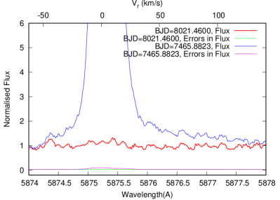
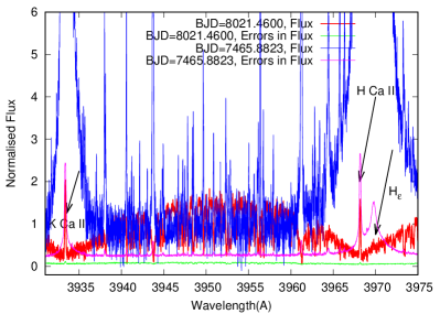
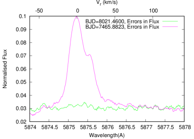
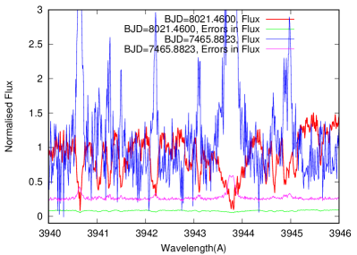
Figure 3: Top-left panel: Observed fluxes of emission lines across He₅₈₇₆spectral region at the dates of minimum and maximum activity, shown by red and blue lines, respectively. Uncertainties of the flux determination are shown by the green and pink colours, respectively. Bottom-left panel: Uncertainties of the flux determinations at the phases of minimum and maximum activity shown in larger scale. Top-right panel: Observed fluxes of emission lines across CaII H and K and H_ϵ spectral regions at the same dates of minimum and maximum activity, shown by red and blue lines, respectively. Bottom-right panel: Part of the observed spectra shown in larger scale. Flux measurement uncertainties are also shown.

4.7 Flare during the night of BJD = 6417

On the night of BJD = 6417 we find a flare of strength 3_ϵ that was fully covered by uniform observations with time steps of 10 min until it recovered its ‘normal’ state. Although 10 min might seem long for flare processes, we can investigate the main stages of this event. Moreover, we are able to simultaneously cover a significant wavelength range containing several emission lines discussed in this work.

On the night of BJD = 6417, we see a flare which started at 6417.6299 (labelled as ‘E₁’ and corresponding to $t$ = $-$34.6 min) and reached its maximum at 6417.65 (i.e. $t$ = 0.0 min, marked as ‘E’ in the top-left panel of Fig. 4). We observe a temporal fading of that flare (BJD = 6417.6841 or $t$ = $+$43.02 min; F₁) and a secondary maximum (secondary flare?) of a strength of 2_ϵ at 6417.69 ($t$ = $+$60.0 min; ‘F’) that later restored to normal state at 6417.7642 ($t$ = 160.00 min, ‘F₂’). In Fig. 4, we show the time mark E₂ (BJD = 6417.6445 $t$ = $-$12.6 min); at this time we see transit from a comparatively slow increase to an avalanche-like increase in flare intensity. The total duration of this flare is about 200 min, i.e.  more than 3h.

This flare is not the strongest in our observational set (Fig. 1). Although this phenomenon may differ from the other strong flares marked with letters ‘B’, ‘C’, and ‘D’ in Fig. 1, we note a few interesting facts:

1. The $H_{\alpha}$ line shows a symmetrical profile (see top-left panel of Fig. 5), as in the case of flares C and D shown in Fig. 2.

2. We see a good correlation between the strength of all lines and the strength of $H_{\alpha}$. We interpret this as all lines most likely forming in one flare space.

3. The cores of all lines are affected by the the self-absorption, suggesting that we see multi-component structures of the absorbing condensed matter.

4. The fine structure of the outer layers affects the cores of all lines shown in Fig. 5. This structure of the outer layers changes with time on short timescales. Indeed, we see differences in the cores of the lines observed at $t$ = $+$43.02 and $+$60.0 mins displayed with pink and cyan lines, respectively, in Fig. 5. Even in the case of the CaII K line, we note a self-absorption component shifted by different $V_{\rm r}$  at different flare stages.

5. We note the self-absorption components in the cores of the CaII and He₅₈₇₆ lines which are moving bluewards and redwards reflecting outward and inward flows of hot matter in the outer atmosphere, respectively (top-right and bottom-left panels of Fig. 5).

6. The multi-component structure of the active regions of the atmosphere is also reflected in the shape of D₁ and D₂ NaI lines. In the ‘quiet’ state, we recognise the absorption components of the cores of emission lines. In the ‘active’ phases the emission line intensity increases and self-absorption becomes notable; see the bottom-right panel of Fig. 5. However, this second emission core forms with another self-absorption component, which we interpret as at least two regions of line formation in the cases of D₁ and D₂.

4.8 Flare activity on BJD = 6718, 6420, and 6426

Other extended and well sampled sets of spectroscopic observations of the Proxima Cen were collected during the nights BJD = 6718, 6420, and 6426. From the comparison of spectral lines in emission obtained at the same times, we may study the physics of the flare variability over short timescales thanks to exposures taken every $\sim$10 min. Hence, we can investigate the relative responses of different lines during flare events.

During those nights, we detect a few flare events covered by exposures made at varying time intervals. We show the changes of $pEW$ of several lines during those nights in Fig. 4. For convenience, the upper x-axis is given in minutes. Time $t$ = 0 min corresponds to the maximum of the flares.

On BJD = 6418, we detect a flare in some lines with a duration of 250 min (top-right panel of Fig. 4). The strength of the flare is of order 2$\epsilon$. We most likely capture part of the flare, which we explain from the weak changes in amplitude of the emission lines and the absence of reaction of the He₅₈₇₆ line. On the other hand, we see the same flare phases, marked with small letters, as on the night of 6417.

On BJD = 6420 and 6426, we detect a flare event of 100 min in duration with a strength of 2_ϵ (bottom-left and bottom-right panels of Fig. 4). Again, we see the secondary flares at $t$ = $+$40 or $+$50 min. Interestingly, on BJD = 6426 we see a flare ‘extended in time’, where the strength of H_ϵ corresponds to the 2_ϵ flare.

It is worth noting again that the behaviour of H_ϵ is more sensitive to the flare events compared with other lines. We suggest that this line is formed mostly in the active region of high temperature. We observe strong changes of the $pEW$ of H_ϵ ; even in the case of the extended flare on BJD = 6418, where changes of $H_{\alpha}$ and other lines are weaker than on the previous night (top-left panel of Fig. 4).

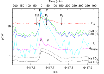
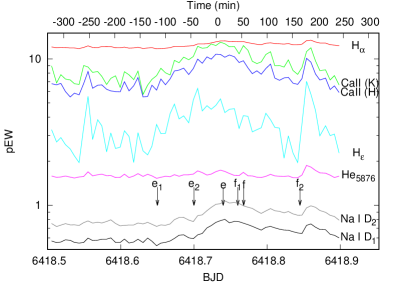
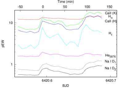
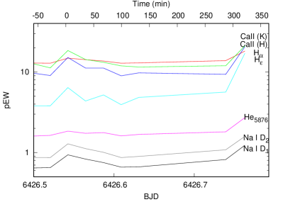
Figure 4: Temporal variations of the $pEW$ of several emission lines during four nights on BJD = 6417, 6418, 6420, and 6426. Time marks with small letters depict the phases of the flare on 6418 corresponding to the same phases as on BJD = 6417.

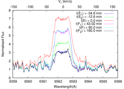
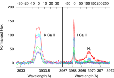
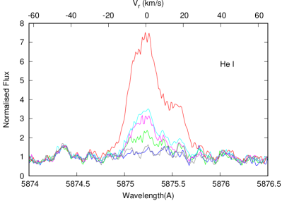
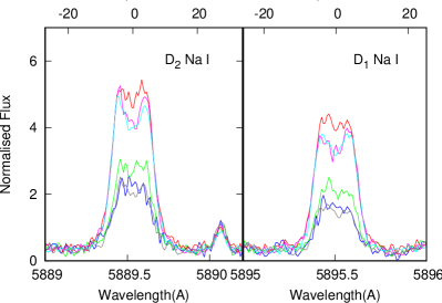
Figure 5: Temporal variations of the $pEW$ of several emission lines during the flare on the night of BJD = 6417. The times depicting the different phases are marked at the top of the top-left panel showing changes in the strength of $H_{\alpha}$.

4.9 Rotational modulation of the chromosphere and the photosphere

Here, we aim at detecting the rotation of the chromosphere of Proxima Cen thanks to the extended sets of HARPS high-resolution spectra. We removed the two flare events and the deviant data points from the $pEW$ dataset of the CaII K line, and subtracted the median values per observing epoch. Otherwise, it is not possible to see the modulation, if it exists, because of the different amplitudes of the line intensity at the different epochs and activity states. The Lomb-Scargle periodogram analysis (Lomb 1976; Scargle 1982) yields no significant strong peak. This is probably because of the artificial noise introduced by the removal of the median values from the original data. However, in the interval 30–1100 days, the highest peak lies at 90.72 days (with an uncertainty of $\pm$1.5 days as derived from the FWHM of the peak). The second-highest peak of the periodogram lies at 81.68 $\pm$ 1.5 days. We note however that the periodogram is rather sensitive to the removal of deviant data. Figure 6 displays the median-subtracted Ca ii K $pEW$ folded in phase with the period of 90.72 days. The data show a sinusoidal modulation with a small amplitude of 1.5Å. A similar sinusoidal pattern is found when using the 81.68-day period, thus making the two periodicities indistinguishable with current HARPS spectra. The two values differ from the rotational period of 116.6 $\pm$ 0.7 days determined from a subset of 222 HARPS spectra included here by Suárez Mascareño et al. (2015), but are closer to the period of $\sim$83 days reported by Benedict et al. (1998), Kiraga & Stepien (2007b), and Wargelin et al. (2017). These latter authors used photometric observations obtained with the Hubble Space Telescope (HST) and the automated sky survey ASAS (Pojmanski 1997; Pojmanski & Maciejewski 2004). A periodicity of 82.6 $\pm$ 0.1 days is also reported by Collins et al. (2017) after combining UVES, HARPS, and ASAS photometry. These authors discussed that the 116.6^d measurement published by Suárez Mascareño et al. (2015) is likely an alias induced by the specific HARPS observation times, and concluded that the most significant rotation period of Proxima Cen is 82.6 $\pm$ 0.1 days.

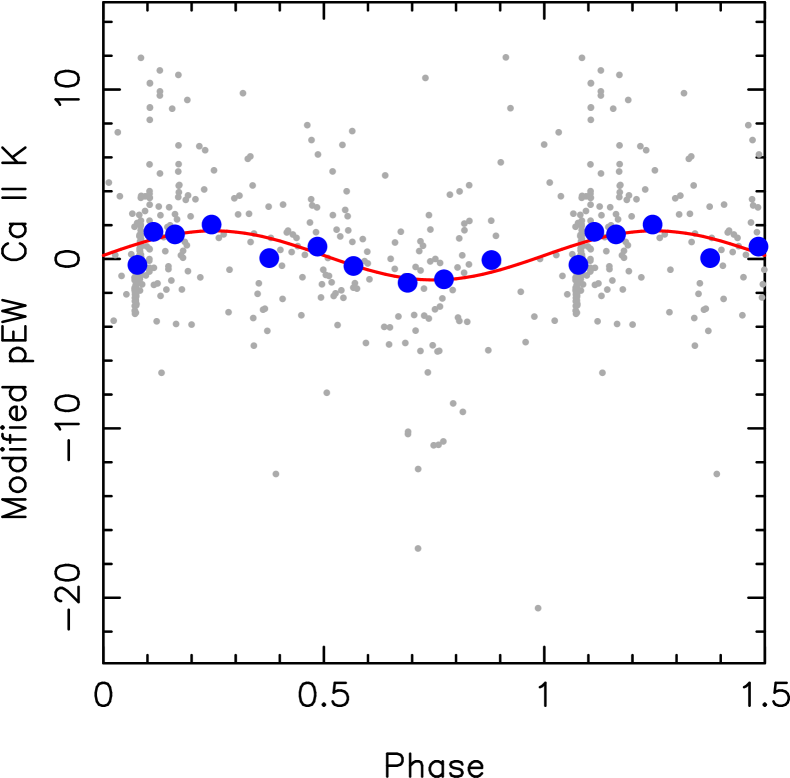
Figure 6: Median-subtracted pEWs of the Ca ii K line (grey dots) folded in phase with the period of 90.72 days. The red line depicts the sinusoidal fit to the folded data (amplitude of 1.5 Å), and the blue dots correspond to the data points averaged with their 21 neighbours. Flares and strongly deviant data points are not included in the diagram.

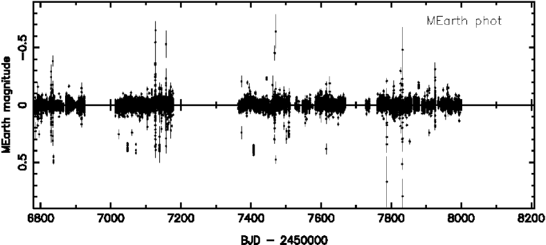
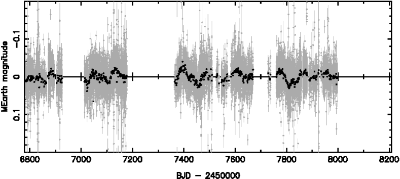
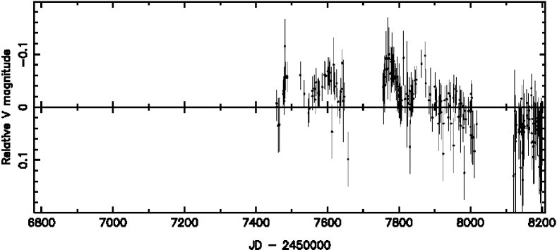
Figure 7: Top: Proxima Cen photometric light curve (filter RG715) delivered by MEarth DR7 (black dots). The data span a period of 3.2 yrs. Negative magnitudes imply brighter states of the star. Middle: Enlargement of the MEarth DR7 light curve. Original data are plotted as grey dots. The day-averaged photometry is shown with black dots. Bottom: ASAS-SN light curve (black dots) spanning a time period of 2 yrs. The mean magnitude of 11.227 mag has been subtracted from the original data for a proper comparison with the MEarth DR7 light curve.

In the recent seventh data release (DR7) of the MEarth project (Berta et al. 2012; Irwin et al. 2011), Proxima Cen is included with more than 64200 photometric magnitudes obtained with the $RG715$ filter between 2014 May and 2017 August. Irwin et al. (2011) provided a detailed review on the observing cadence, exposure times, and processing of the enormous amount of data of the MEarth monitoring campaigns. Concerning Proxima Cen, the resulting MEarth photometric light curve is illustrated in the top panel of Fig. 7, where the data present a dispersion of $\pm$30 mmag, which is three times larger than the typical photometric error bar. A quick inspection of the light curve reveals some sinusoidal patterns with small amplitudes at various epochs (e.g. BJD = 2457400). After applying a 2-$\sigma$ clipping algorithm to remove the most deviant data points, we obtained the Lomb-Scargle periodogram of the MEarth DR7 light curve shown in the top panel of Fig. 8. A strong peak is detected at 91.0 $\pm$ 3.0 days (a second strong peak is seen at $\approx$124 days, but it has a non-negligible contribution from an alias of the 91.0-day peak. This is most likely an alias of the annual window, i.e. $P_{alias}=1/(1/91-1/365)=121^{d}$). Interestingly, the MEarth DR7 periodogram shows quite a number of peaks well above the false-alarm probability (FAP) of 0.1%, suggesting that they may be significant frequencies of the data. We removed the strong 91.0-day periodicity from the original photometry, and a forest of significant peaks still remain in the periodogram. These peaks lie at 39.4, 42.9, 56.9, 83.2, 116.6, 129.2, and 167.3 days (with estimated uncertainty of 1–3 days), and all have associated amplitudes between 3 and 7 mmag (smaller than the quoted amplitude of the 91.0-day peak; see below). We note that two of these frequencies, 83.2 and 116.6 days, are consistent at the 1-$\sigma$ level with those previously reported in the literature using very different datasets (Benedict et al. 1998; Kiraga & Stepien 2007b; Suárez Mascareño et al. 2015; Wargelin et al. 2017; Collins et al. 2017). Therefore, there is little probability they are caused by the way the various data have been acquired. Rather, they may be true signals of the periodic activity of Proxima Cen. The MEarth DR7 data folded in phase with the 91.0-day period are shown in the bottom panel of Fig. 9. A sinusoid curve with an amplitude of 8.7 mmag is plotted on top of the observations.

Figure 8: Top: Lomb-Scargle periodogram of the MEarth DR7 light curve for Proxima Cen. Bottom: Lomb-Scargle periodogram of the ASAS-SN light curve for Proxima Cen after subtraction of the decreasing flux trend. The 0.1% FAP is indicated by the horizontal dashed lines.

Proxima Cen has also been part of the All-Sky Automated Survey for Supernovae (ASAS-SN) long-term photometric monitoring (Shappee et al. 2014). The ASAS-SN $V$-band light curve is shown in the bottom panel of Fig. 7. It overlaps with the MEarth DR7 data and extends over an additional period of several months of observations. Both the MEarth DR7 and ASAS-SN light curves cover a total of 3.9 years of continuous photometric monitoring. There are two obvious features highlighted by the comparison of both light curves: one is that the amplitude of the variations of the ASAS-SN data is larger than that of the MEarth DR7 photometry. This is very likely explained by the fact that the variability of Proxima Cen is more notorious at blue wavelengths. The second feature is that the ASAS-SN photometry shows a decreasing trend towards fainter $V$ magnitudes, which contrasts with the flat nature of the MEarth $RG715$ data. We note that the state of minimum activity labelled with the letter ‘A’ in previous sections corresponds to epochs with the faintest $V$ magnitudes. Whether this trend is real or an artifact of the ASAS-SN data is not clear to us since the two curves were acquired with different filters. The decreasing trend, which is mostly dominated by the most recent epoch of observations, induces a strong signal/power at small frequencies in the Lomb-Scargle periodogram of the ASAS-SN data. To identify potential peaks at longer frequencies, we removed the trend by subtracting a fourth-order polynomial from the original photometry. The resulting Lomb-Scargle periodogram is shown in the bottom panel of Fig. 8, where one strong peak is visible at 96.3 $\pm$ 5.0 days. After removing this signal from the light curve, there remains only one significant peak at 82.8 $\pm$ 4.0 days with a FAP above 0.1%.

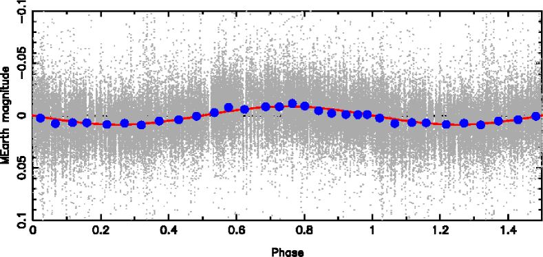
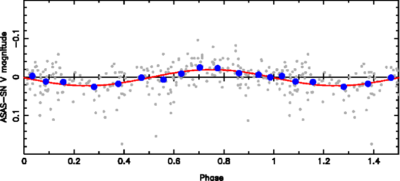
Figure 9: MEarth DR7 (top) and ASAS-SN (bottom) light curves (grey dots) folded with a period of 91.0 and 96.5 d, respectively. The sinusoid fit to the data is shown with the red curve (amplitudes of 8.7 and 21.0 mmag). Each blue dot corresponds to the average of 3000 MEarth and 19 ASAS-SN individual data points. We note that the vertical scale is different by a factor of two different between the two panels.

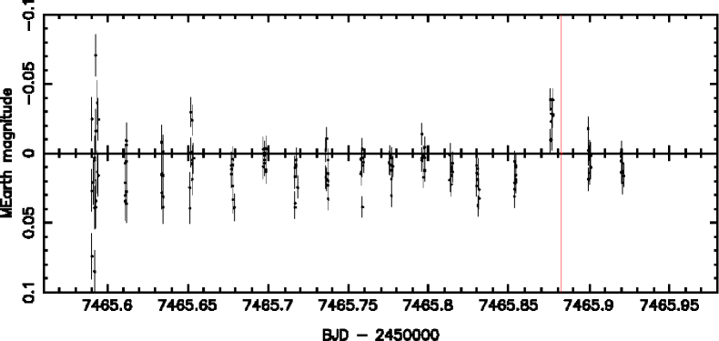
Figure 10: MEarth DR7 light curve of March 18, 2016. The red vertical line indicates the location of the spectroscopic flare B.

Within 1-$\sigma$ of the quoted uncertainties, we found the peaks at $\sim$91 and $\sim$83 days to be common to all three data sets (HARPS, MEarth, and ASAS-SN), with the peak at $\sim$91 days being the strongest signal. These two periodicities are likely related to the rotation period of Proxima Cen. The changes in the variability periods could correspond to changes and evolution (appearance and disappearance) of active regions located at different latitudes on the stellar surface. Proxima Cen shows multiple significant periods, which we interpret as differential rotation. On the other hand, we cannot exclude the possibility that the peaks at $\sim$91 or $\sim$83 days are another alias of the annual window.

The strong flare, event B, reported in previous sections is reasonably well covered by the MEarth data: photometric observations are available before, during, and after the flare. This is the only flare reported here for which there is such temporal coverage in the MEarth DR7 database. Figure 10 depicts the MEarth photometry corresponding to March 18, 2016; the location of the spectroscopic flare is indicated. The flare event induced a photometric increase of $\geq$45 mmag in the brightness of Proxima Cen at red optical wavelengths, which is about nine times greater than the amplitude of the rotation curve.

5 Discussion

In this paper we analyse the flare activity of Proxima Cen using extended sets of HARPS spectra. We inspect the intensity of the $H_{\alpha}$ line to study the ”flare activity”. Pavlenko et al. (2017) showed that the molecular background of the emission lines in the spectrum of Proxima Cen shows rather marginal response to the variations of the activity level. Using this discovery, we computed the $pEW$ of multiple emission lines and present a detailed analysis of the profiles of several emission lines of interest to study dynamic processes occurring during different flare phases. We find some similarities and differences in the temporal changes of $H_{\alpha}$ and other emission lines.

The hydrogen and helium emission lines are of special interest. Indeed, these lines form in the flare region, in layers of high temperature (T $>$ 10000 K) in the inner and/or outer chromosphere, where we observe a large dispersion of velocities in the largest flares. HeI lines form in the regions of higher temperatures and their intensities are rather marginal during the minimum activity of Proxima Cen, contrary to $H_{\alpha}$.

The minima in $pEW$ of $H_{\alpha}$ (‘A’) are just barely fainter than the mean $pEW$, yet the minima in H_ϵ are about ten times lower than the mean $pEW$. This raises the possibility that the blue end of the spectra is prone to very low S/N on certain dates, not that the blue emission lines are actually lower on the star.

The HI emission line H_ϵ disappears almost completely during the minimum activity of Proxima Cen, an effect that cannot be explained by the low S/N on those dates (Sect. 4.6). Indeed, our analysis shows that the S/N in the blue part of the spectra containing CaII H and K and H_ϵ is higher in quiet mode. On the contrary, we see a drop in S/N during phases with strong flares. However, at these dates H_ϵ increases its intensity by several orders of magnitude. Even if the increase of H_ϵ originates from the drop of the background flux formed in the stellar atmospheres the formally computed $pEW$should increase during flares.

We suggest that differences in the physical conditions responsible for the formation of the emission lines in quiet and flare modes may provide a more realistic explanation of these phenomena. Indeed, the Balmer decrement should change in flare mode due to variable physical conditions in the regions where hydrogen forms. A more detailed consideration of this problem is beyond the scope of this paper, but this last possibility cannot be discarded.

Moreover, the formation of the strong emission in the core of the NaI line appears very unusual, as already noted by Pavlenko et al. (2017). Special conditions are needed to create such strong NaI emission. We see that the half-width of the NaI line shows rather marginal changes during flares. At the same time, the intensity of the core of this line reduces in the strong flare modes while some emission appears in the wings.

Our study is based on the analysis of the $pEW$ and emission line profiles of HI, HeI, CaII, and NaI. Firstly, we looked at their correlation with the strength of $H_{\alpha}$. We selected $H_{\alpha}$ as the reference line because it forms in high-temperature (flare) regions. All lines show a good correlation with the strength of $H_{\alpha}$. The He₄₀₂₆ line shows the weakest correlation with $H_{\alpha}$, indicating that the processes and regions of the formation of this line differ from other lines. Interestingly, we note that the other HeI line He₅₈₇₆ better follows $H_{\alpha}$.

From our dataset we selected three dates of minimum and maximum activity of Proxima Cen. During the minimum activity, the spectrum of Proxima Cen does not exhibit any He₅₈₇₆ or He₄₀₂₆ lines. Moreover, the intensity of $H_{\alpha}$ is reduced by a factor of eight with respect to its maximum values, while the intensity of the CaII lines are 150 times lower. We observe an almost complete disappearance of the lines with the highest excitation during the days of absolute minimum of $H_{\alpha}$ on BJD = 8021.4600, 8023.4639, and 8027.4785 (Sect. 4.4). Furthermore, the CaII lines almost disappear, as if the star had lost its chromosphere for a while. This period of minimum activity of the chromosphere may last a few days or possibly weeks. Even the strongest of all lines, H_ϵ, is not seen, although this line is entirely formed in the flare regions, contrary to $H_{\alpha}$ which is still present in the quiet state. The evaporated chromospheric matter in flares becomes cooler during minimum activity, suggesting that the condensed matter absorbs the blue parts of the NaI emission lines. The emission in NaI D₁ and D₂ lines is still present, implying that they likely form in the remnants of the formerly strong chromosphere.

During the periods of strongest activity of Proxima Cen, an extended red wing is present in the $H_{\alpha}$ line, most likely as a result of the hot matter penetrating into the cooler layers. Strong flares affect the formation region of CaII lines and show the anti-correlation with $H_{\alpha}$ (Pavlenko et al. 2017). The intensity of the NaI, D₁, and D₂ lines is reduced during strong flares, but not as much as the CaII lines. Interestingly, different flares yield emission lines of different widths, suggesting that stronger flares occur in the regions of larger turbulent velocity dispersion. Even moderately strong 1_ϵ flares produce the notable He₄₀₂₆ and He₅₈₇₆ lines (Fig. 11). We also emphasise that absorption components are seen in the cores of all lines during maximum activity.

We analysed extended sets of spectra obtained on specific dates where flares of different strengths took place. The study of temporal sequences of $H_{\alpha}$ reveals variability on timescales of 10 min. We observe a few flares at good temporal resolution even though flares may also occur on shorter timescales. All flares show similar structures with several phases, including a slow initialization, a fast phase, a phase of fading, a secondary increase of intensity, followed by another fading phase. Unfortunately, our interpretation of the different phases lacks critical information: Firstly, we do not know the precise geometry and size of flare regions. Secondly, we do not spatially resolve the stellar disc, implying that the spectrum of Proxima Cen includes the integrated flux of the whole stellar surface. Finally, flares may appear at different parts of the stellar disc and even at the limb, or partially beyond the limb. All these cases of potential variability may produce different shapes of the observed lines.

Fortunately, we have at least four full nights with good time coverage where we see different profiles due to activity. On BJD = 6417 we have a flare with a strength of $3_{\epsilon}$ with well-defined temporal behaviour. A similar flare structure may be present on the following day (BJD = 6418), however, the temporal changes here are smoother in time. On the other hand, we see a flare on BJD = 6418, at least seen in the H_ϵ behaviour. These results agree with Davenport et al. (2014) who found that the majority of flares occurring in the atmosphere of the active M4 dwarf GJ 1243 last longer than approximately 30 minutes and show multiple peaks depicting the complex nature of flares.

Nevertheless, we see different behaviour of emission lines formed in the flare regions and the chromosphere. Our analyses suggest the presence of a flare region located over the chromosphere, with both regions being bound by a transition zone. Strong flares penetrate the chromospheric layers and partially destroy them reducing the strength of chromospheric lines. In other words, the structure of the flare region is more complicated than in the case of the Sun. Strong emission in the NaI, D₁, and D₂ lines is present during phases of minimum activity, however this emission is affected by absorption of cooling plasma located in formerly hot regions. We believe that these lines form in the lower chromosphere, as their widths show little variation with the level of activity.

We encourage observers to acquire more continuous HARPS observations over several days/weeks to assess the structure, geometry, and evolution of the flare regions. This strategy should also be extended to other bright M dwarfs in order to compare these patterns in a broader range of sources.

Appendix A A

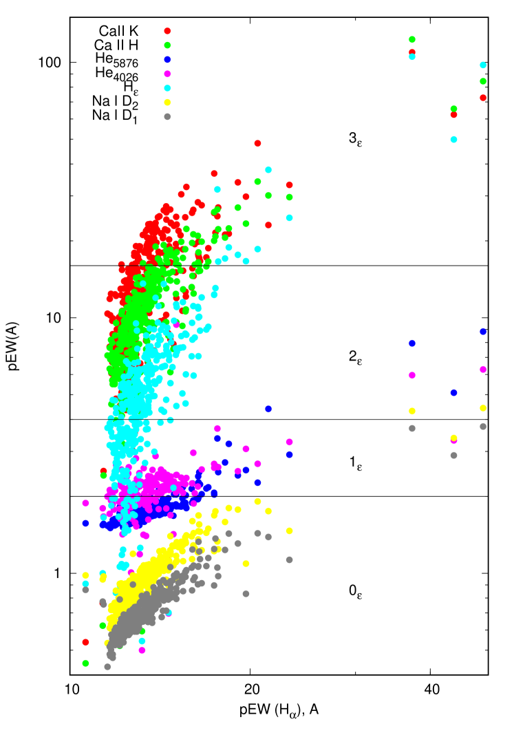
Figure 11: Correlation of the variations in the $pEW$ of some emission lines with the $pEW$ of $H_{\alpha}$ for all dates. The horizontal lines split the figure with respect to our criteria of the strengths of H_ϵ (Section 1).

Table 4: Changes of the $pEW$ of several emission lines

BJD	$H_{\alpha}$	CaII(K)	CaII(H)	He5876	He4026	Hϵ	NaI(D2)	NaI(D1)
3152.5999	12.890	19.066	14.332	1.746	1.969	9.508	0.783	0.616
3202.5847	43.796	62.410	65.757	5.088	2.720	49.893	3.384	2.894
3203.5371	17.684	27.040	22.213	2.487	2.014	16.606	1.243	0.975
3205.5317	15.059	11.952	9.609	1.829	8.572	4.514	0.948	0.794
3207.5051	12.437	5.008	4.611	1.623	0.461	1.937	0.849	0.646
3207.5110	12.436	5.141	4.421	1.636	0.656	2.414	0.769	0.635
3577.4956	12.302	13.018	9.739	1.696	1.509	5.877	0.699	0.560
3809.8936	13.313	18.012	12.005	1.591	1.395	5.211	0.909	0.703
3810.7834	11.656	11.859	7.633	1.513	1.431	3.862	0.611	0.482
3812.7822	11.895	12.353	8.525	1.571	1.469	4.745	0.649	0.524
3816.8096	12.156	12.984	8.804	1.590	1.522	4.935	0.683	0.544
4173.8184	11.678	10.228	6.880	1.505	1.379	3.748	0.610	0.475
4293.5864	12.856	16.315	11.495	1.715	1.577	6.255	0.859	0.661
4296.5933	13.383	14.243	11.246	1.801	1.409	7.216	0.962	0.752
4299.5977	12.689	12.003	9.570	1.626	1.551	4.785	0.818	0.629
4300.5576	13.433	17.932	12.330	1.694	1.519	6.094	0.937	0.737
4646.5693	13.649	19.344	13.608	1.822	1.557	7.357	0.989	0.760
4658.5645	13.239	14.329	10.858	1.687	1.323	5.207	0.923	0.691
4666.5435	12.388	14.018	9.927	1.675	1.544	5.435	0.772	0.607
4878.8638	15.044	24.824	16.890	2.035	1.813	11.295	1.170	0.874
4879.8301	12.316	13.903	9.370	1.612	1.440	4.533	0.747	0.574
4881.8735	12.993	17.230	11.340	1.722	1.589	6.705	0.811	0.617
4882.8535	14.490	24.215	16.839	1.751	1.586	7.478	1.084	0.809
4883.8618	12.937	17.681	13.541	1.652	1.668	8.912	0.784	0.591
4884.8354	12.551	13.546	9.465	1.620	1.384	4.976	0.789	0.605
4885.8750	12.190	16.156	10.349	1.577	1.743	5.487	0.708	0.550
4886.8438	12.254	11.473	7.947	1.602	1.357	4.385	0.720	0.561
4989.6523	14.229	21.399	14.083	1.707	1.460	6.406	0.867	0.674
4992.6504	11.707	12.407	8.193	1.548	1.291	4.038	0.632	0.502
5053.5562	13.055	19.046	14.432	1.677	1.635	6.294	0.908	0.692
5057.5386	12.810	17.949	12.613	1.715	1.618	6.653	0.876	0.683
5275.7715	13.849	21.512	15.388	1.770	1.672	7.411	0.976	0.741
5276.8716	12.699	14.710	10.893	1.631	1.276	4.489	0.794	0.616
5277.8062	12.215	15.401	10.607	1.559	1.434	4.604	0.743	0.578
5278.7905	14.300	20.514	15.465	1.954	1.745	9.308	0.924	0.713
5279.7920	13.347	11.439	9.874	1.707	1.223	4.173	0.986	0.724
5280.7939	13.983	22.077	15.265	1.743	1.444	7.126	1.076	0.820
5281.7598	14.344	26.349	19.259	1.933	1.824	13.570	1.023	0.782
5282.8140	14.923	22.895	17.440	2.036	1.630	9.737	1.278	0.980
5283.7788	12.705	13.590	9.549	1.621	1.395	4.515	0.866	0.663
5292.8027	13.913	16.956	12.184	1.762	1.302	6.342	0.996	0.754
5611.8071	15.581	24.732	18.560	1.890	1.586	8.670	1.384	1.012
5641.7515	13.495	17.931	13.400	1.830	1.570	6.470	0.913	0.709
5644.7910	13.526	17.867	11.860	1.667	1.388	5.601	0.859	0.657
5645.7593	13.720	16.356	12.060	1.727	1.469	6.379	0.840	0.640
5647.7300	37.302	109.430	123.000	7.946	5.102	105.250	4.318	3.691
5648.8286	12.826	15.777	11.225	1.665	1.406	5.034	0.760	0.591
5653.6494	12.629	15.355	11.026	1.693	1.484	6.154	0.749	0.589
5656.6514	11.553	10.381	7.119	1.535	1.320	3.708	0.533	0.431
5659.7778	11.786	9.915	6.983	1.536	1.326	3.157	0.594	0.467
5663.6284	12.289	9.918	7.882	1.605	1.160	3.499	0.666	0.536
5673.7227	11.785	9.952	7.198	1.616	1.380	4.766	0.598	0.482
5715.5605	13.882	16.343	12.489	1.729	1.402	5.511	0.996	0.766
6310.8408	13.167	13.643	11.507	1.669	1.585	4.713	0.899	0.684
6320.8667	16.072	26.470	21.220	1.930	2.258	11.110	1.287	0.942
6322.8281	12.535	14.110	11.043	1.596	1.702	5.558	0.772	0.599
6354.8208	13.840	15.120	11.604	1.684	1.528	4.944	1.009	0.757
6355.8647	14.611	1.183	0.803	1.778	0.314	0.702	0.896	0.797
6356.8047	13.227	14.417	10.664	1.606	1.462	4.596	0.948	0.714
6361.8389	13.061	14.120	11.607	1.601	1.737	5.260	0.851	0.635
6362.8809	13.280	16.030	12.216	1.613	1.848	5.268	0.927	0.706
6363.7783	13.247	15.810	16.343	1.984	3.200	13.605	0.830	0.647
6365.8184	13.902	23.503	19.003	1.938	2.190	11.971	1.046	0.791
6366.7949	12.956	12.878	10.572	1.651	1.600	5.694	0.795	0.599
6367.7729	12.315	11.695	9.746	1.594	1.399	4.983	0.766	0.589
6369.7544	12.357	11.586	8.773	1.577	1.432	5.029	0.724	0.568
6370.7476	12.516	15.564	11.719	1.629	1.686	6.599	0.808	0.614
6371.8052	11.940	12.188	9.538	1.549	1.854	4.436	0.685	0.545
6373.7373	12.520	15.054	11.915	1.605	1.896	5.916	0.808	0.621
6374.7646	12.445	13.615	10.970	1.582	1.620	4.681	0.764	0.596
6417.5044	12.853	6.855	6.137	1.701	7.019	3.242	0.951	0.717
6417.5117	12.499	6.492	5.210	1.617	6.727	1.474	0.918	0.678
6417.5190	13.452	9.492	8.084	1.874	8.070	5.289	1.018	0.786
6417.5264	12.733	6.340	5.064	1.712	7.245	2.227	0.982	0.724
6417.5337	12.335	5.744	4.974	1.633	7.438	1.479	0.884	0.666
6417.5410	12.374	5.840	4.923	1.676	7.502	1.688	0.866	0.658
6417.5483	12.268	5.877	4.896	1.511	7.536	1.237	0.906	0.642
6417.5557	12.128	4.543	4.372	1.608	8.082	0.892	0.899	0.638
6417.5630	12.373	5.897	5.015	1.730	7.739	1.513	0.912	0.652
6417.5703	11.930	4.819	3.972	1.604	7.703	0.839	0.855	0.613
6417.5786	12.394	5.098	5.136	1.668	8.697	1.630	0.910	0.683
6417.5859	12.275	4.520	4.387	1.619	7.164	1.582	0.844	0.650
6417.5933	13.104	5.298	4.300	1.602	6.211	1.258	0.867	0.656
6417.6006	13.057	5.500	5.139	1.542	7.222	2.418	0.887	0.654
6417.6079	13.066	6.437	5.097	1.611	7.572	2.222	0.871	0.655
6417.6152	12.842	5.664	5.000	1.588	7.280	1.831	0.885	0.646
6417.6226	12.407	4.356	4.562	1.659	8.277	1.077	0.847	0.638
6417.6299	12.638	5.648	5.299	1.609	8.611	2.201	0.891	0.629
6417.6372	13.487	6.714	6.816	1.707	6.762	3.669	0.935	0.684
6417.6445	14.596	8.690	8.519	1.967	7.775	7.300	1.027	0.789
6417.6543	21.457	23.078	30.127	4.402	7.785	37.944	1.751	1.387
6417.6621	18.424	21.342	22.382	3.210	7.487	18.869	1.800	1.430
6417.6694	17.499	21.526	20.838	2.626	6.372	13.070	1.748	1.367
6417.6768	16.397	19.851	18.034	2.269	6.457	10.032	1.685	1.329
6417.6841	16.014	15.614	14.593	2.248	6.414	8.208	1.600	1.239
6417.6914	16.443	17.121	16.055	2.486	6.800	10.095	1.554	1.217
6417.6987	16.495	16.682	15.274	2.229	6.534	8.905	1.455	1.136
6417.7056	15.973	13.144	13.186	2.142	6.626	7.071	1.395	1.051
6417.7134	15.619	12.114	10.779	2.020	6.625	6.004	1.314	1.018
6417.7207	15.413	10.649	9.295	1.967	7.584	5.058	1.222	0.932
6417.7280	14.362	9.803	9.452	1.820	6.715	4.288	1.089	0.853
6417.7354	13.835	7.442	6.306	1.773	7.986	2.992	1.087	0.844
6417.7427	13.351	6.348	6.342	1.678	7.495	2.702	1.010	0.735
6417.7505	12.945	5.992	5.181	1.622	7.066	1.960	0.932	0.701
6417.7573	12.703	6.050	6.239	1.627	6.735	1.909	0.890	0.658
6417.7642	12.431	5.184	4.577	1.595	7.311	1.827	0.831	0.630
6417.7720	12.272	6.054	5.173	1.645	7.049	3.017	0.873	0.620
6417.7793	12.314	6.740	5.787	1.653	6.820	3.430	0.820	0.612
6417.7866	12.197	5.113	4.773	1.639	7.520	1.087	0.851	0.637
6417.7939	12.057	4.415	4.326	1.650	7.906	1.667	0.802	0.614
6417.8037	12.602	6.596	6.733	1.705	5.914	3.311	0.853	0.678
6417.8105	12.336	5.492	4.764	1.589	6.410	1.438	0.902	0.672
6417.8179	12.299	6.333	5.437	1.615	7.652	1.738	0.881	0.689
6417.8257	12.176	5.365	4.563	1.583	7.374	0.835	0.914	0.663
6417.8325	12.210	4.888	4.137	1.591	7.637	1.181	0.879	0.662
6417.8403	12.511	5.888	6.523	1.579	7.553	1.472	0.915	0.679
6417.8477	12.509	7.564	5.940	1.612	6.069	1.655	0.870	0.650
6417.8545	12.304	5.414	4.496	1.558	7.006	1.052	0.861	0.655
6417.8623	12.342	7.500	5.274	1.617	7.184	1.745	0.859	0.655
6417.8691	12.297	4.855	4.995	1.561	7.629	1.867	0.883	0.667
6417.8774	12.902	7.207	5.807	1.799	7.253	4.022	0.925	0.719
6417.8848	12.582	7.012	5.415	1.678	6.322	2.917	0.936	0.711
6417.8921	12.764	6.141	5.850	1.762	6.747	2.748	0.973	0.700
6417.8994	12.850	4.932	4.836	1.818	7.729	2.112	0.945	0.717
6417.9072	12.768	6.155	5.552	1.723	6.952	2.760	0.898	0.675
6418.5054	12.067	8.944	6.769	1.588	4.445	3.284	0.753	0.572
6418.5122	11.925	6.859	6.649	1.553	4.131	2.709	0.717	0.557
6418.5181	12.002	7.799	6.805	1.565	4.418	2.904	0.734	0.563
6418.5244	11.957	7.290	5.986	1.587	4.594	2.600	0.751	0.583
6418.5308	11.876	7.188	5.496	1.560	5.016	2.431	0.736	0.577
6418.5366	11.876	6.767	5.841	1.540	4.447	2.177	0.737	0.559
6418.5430	11.771	6.698	5.689	1.563	5.110	1.961	0.730	0.553
6418.5493	11.976	9.011	6.786	1.576	4.718	3.407	0.763	0.558
6418.5552	12.277	8.807	8.210	1.695	5.208	5.551	0.784	0.598
6418.5615	11.980	8.088	6.308	1.591	4.735	2.818	0.758	0.577
6418.5684	11.937	8.199	6.614	1.619	5.907	3.845	0.767	0.579
6418.5742	12.141	7.595	6.646	1.633	5.309	3.488	0.759	0.588
6418.5806	12.148	6.684	6.204	1.595	5.573	2.321	0.777	0.589
6418.5864	12.135	7.366	6.044	1.600	5.415	3.123	0.797	0.600
6418.5928	11.912	7.670	5.983	1.550	5.469	2.448	0.753	0.559
6418.5991	11.931	6.395	5.963	1.553	5.253	2.498	0.726	0.558
6418.6050	12.031	8.181	6.982	1.634	5.479	3.231	0.730	0.589
6418.6113	11.835	7.779	6.049	1.548	5.108	2.958	0.735	0.554
6418.6177	11.884	7.224	6.554	1.588	5.508	1.963	0.735	0.563
6418.6235	12.023	8.266	7.460	1.648	4.903	3.131	0.759	0.588
6418.6304	11.785	5.727	5.501	1.578	4.869	2.354	0.748	0.558
6418.6367	11.876	6.623	5.548	1.631	6.465	2.213	0.767	0.599
6418.6426	11.933	7.250	6.622	1.592	5.275	2.534	0.744	0.570
6418.6489	11.717	7.685	6.122	1.531	5.108	3.569	0.719	0.531
6418.6548	11.783	8.633	7.294	1.556	4.446	3.094	0.737	0.553
6418.6611	11.821	8.038	6.659	1.581	4.921	3.103	0.732	0.560
6418.6675	11.934	7.770	7.309	1.569	5.509	4.237	0.748	0.572
6418.6733	12.179	9.773	8.277	1.621	4.194	4.917	0.799	0.595
6418.6797	12.179	9.419	8.385	1.582	4.461	3.895	0.827	0.626
6418.6860	12.177	10.281	8.647	1.617	4.522	4.084	0.828	0.631
6418.6929	12.246	9.867	7.818	1.619	4.350	3.663	0.795	0.601
6418.6992	12.321	10.394	8.596	1.636	4.731	5.253	0.776	0.593
6418.7051	12.652	12.186	9.971	1.721	4.857	6.292	0.850	0.630
6418.7114	12.650	11.822	9.333	1.674	4.986	4.413	0.863	0.644
6418.7178	12.676	11.919	10.329	1.611	4.680	4.794	0.920	0.702
6418.7236	12.855	12.650	9.961	1.636	4.705	4.536	0.969	0.728
6418.7300	13.086	12.344	10.772	1.699	5.338	4.818	1.018	0.766
6418.7363	13.261	12.998	10.733	1.740	5.023	5.336	1.028	0.787
6418.7422	13.279	12.699	10.263	1.706	4.814	4.305	1.074	0.803
6418.7485	13.162	12.099	10.639	1.652	5.253	4.528	1.039	0.761
6418.7554	13.172	12.160	10.341	1.602	4.662	4.575	1.047	0.778
6418.7617	13.126	10.839	9.453	1.599	4.853	3.349	1.031	0.774
6418.7676	13.126	12.320	9.717	1.681	4.498	4.098	0.994	0.757
6418.7739	12.905	11.456	8.680	1.594	4.556	4.054	0.972	0.739
6418.7798	12.747	9.631	7.932	1.589	4.407	3.174	0.953	0.720
6418.7861	12.591	9.287	8.290	1.557	4.808	3.289	0.914	0.698
6418.7920	12.507	9.545	7.859	1.550	4.443	3.388	0.882	0.678
6418.7983	12.791	10.716	8.603	1.580	4.430	4.255	0.917	0.709
6418.8047	12.878	11.202	9.215	1.630	4.437	3.846	0.952	0.719
6418.8105	12.736	8.995	7.406	1.591	5.435	3.415	0.921	0.704
6418.8169	12.674	9.014	7.140	1.582	5.219	3.373	0.912	0.689
6418.8232	12.613	8.791	7.416	1.576	5.316	2.100	0.890	0.679
6418.8291	12.734	9.851	7.487	1.590	4.870	2.985	0.909	0.678
6418.8354	12.492	8.331	6.829	1.547	5.051	2.279	0.876	0.662
6418.8418	12.497	7.842	6.707	1.545	4.501	1.962	0.857	0.649
6418.8477	12.607	8.741	7.328	1.612	5.512	3.593	0.858	0.643
6418.8540	13.325	11.225	10.094	1.876	5.171	7.026	0.963	0.731
6418.8599	13.431	11.912	9.502	1.827	4.814	5.744	0.994	0.747
6418.8662	13.049	9.691	7.886	1.735	5.056	4.449	0.970	0.710
6418.8721	12.846	8.328	7.180	1.668	5.190	2.984	0.924	0.685
6418.8799	12.825	8.414	7.392	1.661	5.368	3.496	0.898	0.682
6418.8862	12.514	7.183	6.179	1.610	5.244	2.995	0.856	0.635
6418.8921	12.414	7.691	6.550	1.551	5.235	3.067	0.840	0.626
6418.8984	12.328	6.648	5.903	1.584	5.635	2.281	0.793	0.600
6419.6675	12.727	10.426	8.272	1.635	4.766	3.976	0.887	0.660
6419.6738	12.893	11.290	9.688	1.674	4.876	5.829	0.865	0.642
6420.5552	12.127	8.202	6.737	1.584	4.671	2.927	0.772	0.577
6420.5615	12.058	7.492	6.163	1.598	5.030	2.372	0.754	0.571
6420.5688	11.882	6.849	5.898	1.539	5.454	2.507	0.749	0.559
6420.5747	11.933	7.067	6.253	1.587	5.434	2.970	0.732	0.562
6420.5811	11.863	6.915	5.730	1.547	4.811	2.431	0.715	0.549
6420.5874	11.891	7.584	6.115	1.570	5.383	3.013	0.716	0.563
6420.5933	13.629	13.173	11.070	1.986	4.431	7.729	0.982	0.774
6420.5996	13.180	11.443	10.267	1.841	5.316	4.943	1.049	0.816
6420.6055	12.918	11.598	9.585	1.721	5.656	4.327	0.956	0.739
6420.6118	12.649	9.849	9.001	1.770	5.819	4.955	0.893	0.687
6420.6182	12.882	11.196	9.620	1.760	4.597	5.397	0.908	0.689
6420.6240	12.681	10.793	8.875	1.679	5.482	4.007	0.863	0.656
6420.6309	12.242	8.165	6.951	1.570	5.237	2.890	0.800	0.619
6420.6372	12.172	8.884	6.747	1.610	5.196	3.517	0.766	0.576
6420.6436	12.188	8.936	6.992	1.586	4.700	3.367	0.769	0.594
6420.6494	12.056	9.223	7.058	1.573	4.546	2.697	0.748	0.581
6420.6558	12.408	11.212	9.149	1.681	4.315	6.759	0.786	0.603
6420.6616	13.588	15.807	13.646	1.842	4.140	9.089	1.012	0.767
6420.6680	14.089	17.955	14.921	1.804	4.655	7.080	1.131	0.864
6420.6738	13.790	16.518	13.525	1.712	4.652	6.342	1.130	0.883
6420.6802	14.317	17.979	15.046	1.745	4.720	6.448	1.228	0.940
6420.6865	14.107	16.544	12.886	1.691	4.564	5.793	1.219	0.920
6421.5015	11.727	6.065	4.591	1.558	6.548	1.842	0.744	0.575
6421.5078	12.106	7.072	5.765	1.719	5.916	3.677	0.774	0.584
6422.4927	13.462	10.689	8.858	1.726	6.435	3.206	1.007	0.745
6422.7227	16.900	17.240	15.889	2.148	6.350	8.999	1.441	1.067
6422.7305	17.029	18.719	16.591	2.172	6.382	9.224	1.494	1.148
6422.7383	16.389	17.486	15.222	1.974	6.530	7.077	1.460	1.066
6422.7466	15.601	12.640	10.600	1.839	5.419	4.620	1.332	0.968
6423.5220	12.878	8.877	7.812	1.701	5.379	3.295	0.865	0.640
6423.8257	16.376	17.757	16.482	2.396	6.796	10.876	1.359	1.061
6424.4878	12.240	7.157	5.594	1.648	6.389	3.396	0.822	0.629
6424.4956	12.267	6.994	6.380	1.620	6.119	2.428	0.816	0.610
6424.6519	12.222	10.645	8.304	1.657	4.777	4.423	0.781	0.589
6426.4980	12.926	12.753	9.698	1.600	4.570	3.798	0.870	0.644
6426.5205	12.842	11.242	9.050	1.636	4.677	3.806	0.867	0.650
6426.5425	14.837	18.459	15.145	1.846	5.637	6.409	1.284	0.938
6426.5645	14.218	14.295	11.192	1.735	4.804	4.366	1.120	0.832
6426.5869	13.671	13.191	11.188	1.768	5.246	5.193	1.008	0.752
6426.6089	12.849	11.913	8.972	1.611	4.956	3.935	0.868	0.660
6426.6309	12.981	11.530	9.750	1.681	5.572	4.836	0.896	0.665
6426.7393	13.827	11.956	9.359	1.811	6.531	5.636	1.083	0.819
6426.7632	18.156	21.164	20.598	2.715	6.895	17.063	1.589	1.234
6427.4824	12.437	7.664	6.408	1.566	6.006	2.521	0.777	0.587
6427.4990	12.869	8.074	7.317	1.817	6.282	4.623	0.875	0.642
6428.4985	12.674	6.867	6.705	1.689	6.479	2.195	0.885	0.674
6428.5283	13.394	11.346	8.836	1.661	5.772	3.657	0.965	0.705
6656.8022	12.774	14.599	11.017	1.606	1.349	4.527	0.807	0.608
6656.8154	12.695	10.841	9.241	1.633	1.133	4.030	0.793	0.594
6657.8018	12.705	16.110	10.999	1.573	1.390	4.765	0.781	0.595
6657.8169	12.606	14.394	10.067	1.574	1.562	4.294	0.756	0.585
6658.8120	16.358	28.313	20.938	1.951	1.707	11.035	1.208	0.905
6658.8271	15.999	25.759	19.644	1.888	1.610	9.561	1.137	0.858
6659.8232	12.598	14.926	11.102	1.621	1.440	5.130	0.755	0.583
6659.8379	12.991	16.808	12.266	1.642	1.406	5.959	0.843	0.641
6660.8032	13.135	12.094	9.993	1.631	1.332	4.715	0.820	0.646
6660.8574	12.976	15.067	11.119	1.605	1.403	4.712	0.836	0.644
6661.8062	12.538	12.263	9.347	1.565	1.440	3.529	0.752	0.574
6661.8511	12.683	14.837	10.835	1.589	1.361	4.678	0.803	0.624
6663.8560	13.555	18.862	13.991	1.855	1.362	7.636	0.914	0.695
6663.8706	14.059	18.137	14.756	2.108	1.742	11.117	1.008	0.792
6665.7827	13.570	16.283	12.602	1.749	1.370	6.128	0.925	0.704
6665.8130	13.263	11.411	8.948	1.594	1.114	4.221	0.922	0.685
6665.8672	14.647	19.055	14.913	1.842	1.568	7.089	1.120	0.831
6666.7861	13.500	14.258	11.316	1.630	1.242	4.886	0.881	0.645
6666.8164	13.738	17.160	14.352	1.834	1.836	8.392	0.861	0.667
6666.8623	13.043	16.767	11.546	1.607	1.255	4.806	0.807	0.612
6667.7803	12.680	14.746	11.277	1.606	1.544	5.246	0.841	0.636
6667.8291	13.529	19.423	13.997	1.659	1.510	5.955	0.976	0.739
6667.8628	12.993	17.311	11.537	1.581	1.608	5.218	0.842	0.644
7406.8706	19.677	29.783	23.379	2.535	2.321	16.663	1.092	0.831
7407.8618	13.193	0.021	0.594	1.771	0.291	0.543	0.910	0.693
7410.8677	15.438	18.531	17.151	2.173	1.743	11.524	1.290	0.979
7412.8672	13.485	19.634	13.432	1.674	1.526	6.076	0.964	0.723
7413.8696	13.543	18.554	13.554	1.707	1.524	6.199	0.925	0.688
7414.8706	14.302	20.918	15.038	1.798	1.544	7.129	1.065	0.797
7415.8789	13.451	20.635	14.148	1.692	1.610	6.324	0.945	0.707
7416.8721	15.649	32.510	22.279	1.800	1.669	8.581	1.408	1.029
7417.8789	13.687	19.669	13.204	1.704	1.545	6.018	0.948	0.699
7418.8750	20.585	48.212	34.128	2.263	2.041	18.567	1.911	1.434
7420.8760	13.520	23.220	15.779	1.770	1.734	7.424	1.012	0.759
7420.8906	13.084	18.458	12.158	1.655	1.581	5.477	0.911	0.688
7421.8799	13.232	21.094	14.027	1.690	1.570	6.300	0.915	0.684
7422.8677	13.896	22.625	15.241	1.751	1.688	7.241	0.971	0.727
7423.8765	13.604	23.280	15.605	1.747	1.610	7.227	1.015	0.750
7425.8828	13.718	21.646	14.212	1.674	1.699	6.185	0.997	0.744
7427.8833	17.418	36.709	25.927	2.033	1.903	12.332	1.685	1.245
7428.8804	14.479	27.294	18.344	1.816	1.708	8.753	1.163	0.849
7429.8818	14.028	24.742	17.070	1.865	1.748	9.581	1.012	0.760
7431.8872	14.489	25.869	17.377	1.769	1.641	7.762	1.086	0.799
7432.8833	13.396	21.882	14.051	1.676	1.527	6.303	0.966	0.715
7433.8911	13.726	22.090	15.388	1.727	1.648	7.140	1.049	0.795
7434.8799	12.807	17.495	11.918	1.645	1.522	5.703	0.856	0.649
7436.8589	13.634	23.268	15.813	1.721	1.678	7.531	0.959	0.726
7437.8618	15.345	30.427	19.847	1.825	1.677	8.480	1.329	0.972
7438.8579	14.705	26.546	18.489	1.840	1.618	8.542	1.230	0.907
7439.8579	14.107	24.974	16.776	1.774	1.687	8.197	1.092	0.818
7440.8628	13.408	18.581	13.578	1.810	1.582	8.531	0.978	0.732
7442.8687	14.064	16.390	13.015	1.892	1.733	8.505	1.058	0.795
7444.8872	19.078	33.895	27.008	2.415	1.874	17.630	1.774	1.308
7445.8706	14.645	20.241	14.068	1.779	1.486	6.832	1.109	0.815
7446.8716	14.415	22.201	14.869	1.717	1.471	6.486	1.102	0.805
7447.8765	15.303	21.047	15.326	1.826	1.527	7.638	1.268	0.927
7448.8804	15.180	21.885	16.069	1.830	1.624	7.598	1.265	0.917
7449.8760	13.594	17.315	12.678	1.799	1.529	6.562	1.057	0.783
7450.8975	15.073	23.171	18.062	2.120	1.796	11.023	1.324	0.999
7452.8789	13.465	22.219	14.870	1.722	1.567	6.889	0.978	0.731
7453.9116	13.558	18.365	12.928	1.653	1.462	5.412	1.084	0.798
7454.9087	13.950	19.692	14.563	1.735	1.647	6.815	1.109	0.817
7455.9092	17.411	25.719	20.024	2.066	1.967	12.293	1.221	0.897
7456.9082	13.642	18.608	13.181	1.677	1.575	6.049	0.997	0.734
7457.8818	14.545	21.970	16.394	1.876	1.800	9.142	1.068	0.792
7458.8984	14.735	23.535	18.004	1.842	1.735	8.482	1.186	0.874
7460.8833	13.435	19.209	13.353	1.694	1.610	6.402	0.949	0.705
7461.8843	16.599	27.590	19.851	2.041	1.895	12.016	1.231	0.915
7462.8882	13.630	20.506	15.272	1.783	1.765	7.526	1.022	0.760
7463.8901	15.037	19.436	16.241	1.855	1.474	7.596	1.282	0.970
7465.8823	49.008	72.685	84.356	8.833	5.388	97.632	4.435	3.754
7466.9131	13.074	16.625	12.239	1.704	1.509	6.172	0.913	0.702
7467.9097	12.795	15.592	11.283	1.619	1.431	5.319	0.869	0.654
7473.8726	12.828	3.548	3.918	1.708	1.214	1.686	0.906	0.738
7473.8926	12.483	8.239	6.561	1.606	1.261	3.193	0.810	0.621
7474.8945	14.192	21.417	16.216	1.868	1.837	8.964	1.109	0.831
7475.8921	12.558	13.939	10.013	1.636	1.521	5.193	0.813	0.622
7476.8892	12.957	15.540	11.992	1.763	1.484	7.566	0.831	0.635
7477.8979	12.862	15.174	11.055	1.657	1.471	5.576	0.838	0.647
7905.4707	17.631	24.980	26.565	3.370	2.950	31.806	1.332	1.053
7905.5288	15.026	15.060	12.403	1.861	1.510	7.160	1.105	0.836
7905.6182	15.089	18.555	13.867	1.841	1.601	7.367	1.119	0.845
7934.6421	14.166	9.700	8.195	1.699	1.590	3.892	1.163	0.883
7935.6562	13.512	11.040	9.451	1.653	1.326	4.540	0.971	0.721
7936.6221	13.720	11.755	9.573	1.709	1.447	4.931	0.951	0.725
7937.6421	12.714	7.830	6.815	1.627	1.185	3.579	0.854	0.649
7942.5752	13.320	13.798	10.690	1.668	1.543	5.151	0.896	0.694
7943.5610	12.488	12.904	9.937	1.655	1.275	4.689	0.787	0.619
7944.5454	14.017	17.246	14.003	1.799	1.453	7.837	1.047	0.795
7945.5918	14.759	23.442	17.556	1.808	1.551	8.028	1.073	0.804
7946.5405	13.821	20.436	14.644	1.742	1.711	7.403	0.934	0.721
7948.6543	13.514	9.600	8.859	1.749	1.210	4.431	0.991	0.753
7949.6699	13.106	6.627	6.111	1.755	0.496	3.067	0.923	0.711
7951.4634	13.403	8.135	7.531	1.805	1.034	4.383	0.902	0.674
7952.6406	12.857	11.536	9.361	1.615	1.038	4.127	0.776	0.602
7953.4731	13.517	18.296	14.287	1.787	1.748	7.715	0.940	0.722
7954.6279	14.484	16.052	13.038	1.786	1.312	7.713	0.944	0.714
7955.6372	14.889	7.890	7.555	1.680	1.088	2.161	1.073	0.830
7956.4727	13.095	19.019	13.453	1.707	1.583	6.245	0.828	0.646
7959.4731	12.593	14.209	10.473	1.711	1.374	6.010	0.786	0.603
7960.4629	12.643	13.662	10.526	1.607	1.388	4.897	0.865	0.677
7961.4854	12.074	10.035	7.928	1.624	1.421	3.889	0.703	0.549
7962.4712	12.171	12.274	9.099	1.675	1.593	5.346	0.727	0.556
7964.4727	12.108	7.860	6.688	1.592	1.199	3.406	0.697	0.523
7965.4761	12.650	4.817	4.796	1.672	0.719	2.215	0.823	0.648
7966.4746	11.771	9.732	7.981	1.552	1.342	3.425	0.673	0.530
7967.5088	14.478	10.267	9.621	1.807	0.793	4.776	1.190	0.916
7968.4785	11.648	7.700	6.316	1.554	1.179	3.173	0.664	0.517
7969.4712	12.540	11.756	9.341	1.651	1.394	4.562	0.801	0.611
7970.4761	12.904	15.024	10.904	1.680	1.525	6.111	0.828	0.633
7971.4668	12.553	14.052	10.386	1.671	1.467	5.330	0.820	0.646
7972.4653	13.630	15.064	11.640	1.751	1.541	6.320	0.991	0.754
7973.4653	13.570	10.449	9.530	1.685	1.264	4.259	1.008	0.782
7974.4624	14.147	17.958	13.729	1.874	1.582	8.179	1.049	0.808
7979.4590	13.414	10.904	8.243	1.632	1.427	3.882	0.949	0.735
7980.4609	13.432	15.123	11.394	1.801	1.544	6.347	1.077	0.828
7981.5054	15.453	15.274	12.928	1.875	1.501	7.663	1.115	0.851
7984.5039	13.538	13.041	11.668	1.719	1.397	4.723	0.979	0.749
7985.5034	12.895	10.103	8.333	1.633	1.389	3.652	0.870	0.660
7986.5156	23.263	33.132	29.664	2.912	2.514	24.623	1.465	1.129
7987.5249	13.465	14.628	11.889	1.727	1.403	5.739	0.977	0.747
7990.4902	13.813	14.746	13.084	1.907	1.441	9.011	1.017	0.788
7991.5078	13.537	13.213	10.777	1.676	1.329	4.907	0.954	0.710
7992.5029	12.787	12.982	10.182	1.632	1.554	4.451	0.869	0.671
7993.4897	12.409	12.295	9.991	1.644	1.586	5.471	0.787	0.619
7994.4746	12.645	10.458	8.650	1.653	1.217	4.652	0.825	0.638
7995.4780	16.158	19.434	16.153	1.936	1.463	8.375	1.254	0.964
7996.4805	14.066	14.697	12.151	1.737	1.221	5.677	0.993	0.753
7997.4678	16.093	14.582	12.443	1.883	1.238	5.941	1.437	1.072
7998.4819	12.367	10.043	8.047	1.580	1.149	3.560	0.758	0.582
7999.4756	12.238	3.638	3.217	1.769	1.008	2.520	0.834	0.642
8000.4780	13.079	10.159	8.924	1.667	0.882	3.857	0.947	0.711
8001.4912	12.608	13.270	9.891	1.633	1.234	4.665	0.826	0.622
8002.4766	12.514	9.687	8.363	1.726	1.421	4.683	0.788	0.615
8007.5283	12.666	6.580	7.267	1.686	1.008	3.024	0.930	0.708
8011.4893	14.721	16.474	13.983	1.777	1.230	5.549	1.215	0.930
8012.4766	12.905	7.497	6.946	1.768	0.995	4.465	0.904	0.687
8013.4751	13.084	10.954	9.233	1.766	1.444	4.668	0.933	0.716
8017.4683	14.716	8.229	6.129	1.833	1.478	3.972	1.398	1.058
8018.5127	12.994	12.005	10.280	1.676	1.550	5.589	0.860	0.662
8019.4790	12.143	9.785	7.503	1.580	1.178	3.529	0.729	0.565
8020.4834	11.836	8.020	6.802	1.584	1.321	3.174	0.668	0.533
8021.4600	10.618	0.537	0.444	1.569	1.194	0.909	0.982	0.862
8022.4614	12.113	0.563	0.520	1.818	1.207	1.061	0.910	0.790
8023.4639	11.342	0.764	0.624	1.546	1.143	1.000	0.946	0.775
8025.4741	12.738	3.012	2.120	1.676	1.238	1.706	1.192	0.903
8026.4785	12.453	8.081	7.296	1.633	1.417	3.708	0.886	0.688
8027.4785	11.379	2.514	2.416	1.560	1.213	1.655	0.973	0.755