Statics and Dynamics of Polymeric Droplets on Chemically Homogeneous and Heterogeneous Substrates

Abstract

We present a molecular dynamics study of the motion of cylindrical polymer droplets on striped surfaces. We first consider the equilibrium properties of droplets on different surfaces, we show that for small stripes the Cassie-Baxter equation gives a good approximation of the equilibrium contact angle. As the stripe width becomes non-negligible compared to the dimension of the droplets, the droplet has to deform significantly to minimize its free energy, this results in a smaller value of the contact angle than the continuum model predicts. We then evaluate the slip length, and thus the damping coefficient as a function of the stripe width. For very small stripes, the heterogeneous surface behaves as an effective surface, with the same damping as an homogeneous surface with the same contact angle. However, as the stripe width increases, damping at the surface increases until reaching a plateau. Afterwards, we study the dynamics of droplets under a bulk force. We show that if the stripes are large enough the droplets are pinned until a critical acceleration. The critical acceleration increases linearly with stripe width. For large enough accelerations, the average velocity increases linearly with the acceleration, we show that it can then be predicted by a model depending only the size of droplet, viscosity and slip length. We show that the velocity of the droplet varies sinusoidally as a function of its position on the substrate. On the other hand, for accelerations just above the depinning acceleration we observe a characteristic stick-slip motion, with successive pinnings and depinnings.

I Introduction

The wetting behaviors of liquid volumes ranging from micro-/nano-liters to picoliters in microchannels are of great importance for designing droplet-based micro-/nano-fluidic devices Squires and Quake (2005); Seemann et al. (2012); ter Schiphorst et al. (2018) such as DNA-chips, Dugas, Broutin, and Souteyrand (2005) Lab On A CD, Kong et al. (2016) inkjet printing technology, Zhou et al. (2017) or in situ investigation of fibrin networksEvans et al. (2009). Accordingly, equilibrium and dynamic wetting behaviors of liquid drops on smooth (ideal, homogeneous, flat), chemically rough/structured, and topologically patterned substrates has been studied for decades. Furmidge (1962); Lenz and Lipowsky (1998); Gau et al. (1999); Darhuber and Troian (2005); Servantie and Müller (2008a); Jullien et al. (2009); L.-Aguilar et al. (2011); Duprat et al. (2012); Amini et al. (2013); Yao et al. (2013)

FurmidgeFurmidge (1962) showed that the movement of spray liquids on different substrates depends on the droplet’s size, inclination of the substrate, the surface tension of the drop, and the advancing and receding contact angles. Gau et al. (Gau et al., 1999) showed that a shape instability (a bulge state), unlike a Rayleigh Plateau instability, can be employed for all liquids on all striped substrates if the hydrophilic stripes’ contact angles are small enough and if these stripes are long enough. They mentioned that these bulge states could be used to build two-dimensional microchannel networks and hence to construct microbridges, microchips, and microreactors.

To date many experimental,Schaffer and Wong (1998); Léopoldès and Bucknall (2005); Tavana et al. (2006); Maheshwari et al. (2008); Orejon, Sefiane, and Shanahan (2011); Mirsaidov et al. (2012); Yeong et al. (2015) computational and theoretical Shanahan (1995); Thiele and Knobloch (2006a, b); Kusumaatmaja et al. (2006); Kusumaatmaja and Yeomans (2007); Wang, Qian, and Sheng (2008); Qian et al. (2009); Beltrame, Hänggi, and Thiele (2009); Herde et al. (2012); Varagnolo et al. (2013); *SbragagliaM_PRE89_2014; Wang and Wu (2015); Zhang, Müller-Plathe, and Leroy (2015); Liu and Chen (2017) studies on the dynamic wetting behavior of droplets on textured/rough surfaces have shown that a stick-slip type of microscopic slipping is a common behavior.

Schäffer and Wong Schaffer and Wong (1998) showed that the surface roughness is a key factor in pinning of water in glass capillaries. Léopoldès and Bucknall (Léopoldès and Bucknall, 2005) studied the spreading of droplets on chemically heterogeneous striped substrates. In an intermediate regime, they observed a stick-slip behavior, in other words a sudden hopping of the drop while crossing the boundary of two adjacent stripes with different wettability. Tavana et al.(Tavana et al., 2006) investigated a number of chemically different organic ($n$-alkanes) drops on two distinct polymeric films. The observed that on the homogeneous surfaces, all of the liquids move smoothly, whereas on the heterogeneous polymeric films, liquids which have compounds with short-chains present a stick-slip behavior. They noted that the cause of this stick-slip pattern is the varying adsorption of vapor molecules on these polymer films. Maheshwari et al.(Maheshwari et al., 2008) observed a stepwise (discontinuous) pinning-depinning cyclic behavior and multiring stain-formations of the droplets of aqueous DNA solutions at high and intermediate DNA concentrations. Orejon et al.(Orejon, Sefiane, and Shanahan, 2011) observed that the magnitude of the stick-slip motion depends on the concentration of titanium dioxide nanoparticles inside the water drops on different hydrophobic substrates. Yeong et al.(Yeong et al., 2015) experimentally investigated microscopic receding three-phase contact line dynamics of water droplets on superhydrophobic substrates with regular textured pillars and with nanocomposite coatings at micron-time/length scales. They proposed that the microscopic receding contact line’s dynamic on these surfaces looks like ‘a slide-snap behavior’. In this motion, the receding contact line keeps on moving on the top surface of a pillar until snapping to the adjacent pillar in contrast to a stick and slip motion in which the microscopic receding contact lines stay pinned (stick) before jumping into the consecutive locations.

Numerical and/or theoretical investigations into these dynamic behaviors can also be summarized as the following. Shanahan (Shanahan, 1995) calculated the excess free energy per unit length of the three-phase contact line of a spherical evaporating droplet on an ideal solid surface by taking into account the solid-liquid, solid-vapor, and liquid-vapor interfacial free energies of this system. The system must overcome this potential energy barrier so that the triple line can jump to its next static anchored position after this pinning state in which case the contact radius of the drop remains constant while the contact angle and the volume of the droplet decreases. Thiele and Knobloch,(Thiele and Knobloch, 2006b, a) and Beltrame et al. (Beltrame, Hänggi, and Thiele, 2009) modeled pinning/depinning cycle of moving two- and/or three-dimensional mesoscopic droplets with a wetting layer on heterogeneous surfaces by solving the Navier-Stokes equation within the lubrication approximation. (Oron, Davis, and Bankoff, 1997) Kusumaatmaja and co-workers (Kusumaatmaja et al., 2006; Kusumaatmaja and Yeomans, 2007) described equilibrium properties of liquid droplets on substrates with different wettability strengths thanks to the Landau free energy. (Briant, Wagner, and Yeomans, 2004; *BriantAJYeomansJM_PRE69_2004_II) The free energy they choose causes a liquid droplet to coexist with its vapor phase. They computed the dynamic properties of the liquid drops by solving the continuity and the Navier-Stokes hydrodynamic equations of motion with free-energy lattice Boltzmann (LB) numerical simulation technique. (Briant, Wagner, and Yeomans, 2004; *BriantAJYeomansJM_PRE69_2004_II) Wang et al. (Wang, Qian, and Sheng, 2008) carried on continuum simulations of contact line dynamics of a binary fluid flowing between two chemically patterned solid substrates using a diffuse-interface model with the generalized Navier boundary condition. In this model they solved numerically two coupled equations of motion which consist of the convection-diffusion equation for a field variable and the Navier-Stokes equation with a capillary force density. Their simulation results showed an oscillatory (stick-slip) behavior of the interface of the two immiscible fluids on the substrate. Qian et al. (Qian et al., 2009) used both Molecular Dynamics simulations (MD) and a continuum model to investigate the nanoscale-hydrodynamics of the moving contact line on chemically striped surfaces. They observed a stick-slip motion of the contact line on these substrates. Herde et al. (Herde et al., 2012) studied the depinning/repinning dynamics of two-dimensional drops driven by a lateral body force on chemically heterogeneous flat surfaces having periodic (sinusoidal) wetting energy. They solved the Navier Stokes equation for small Reynolds numbers numerically using a boundary element method. Sbragaglia and co-workers (Varagnolo et al., 2013; *SbragagliaM_PRE89_2014) observed a stick-slip periodic behavior of liquid drops sliding over solid substrates patterned with parallel stripes of varying wettability degrees both experimentally and numerically in two dimensions. They solved the diffuse-interface Navier-Stokes equations of motion for a binary mixture using LB simulation method. Wang and Wu (Wang and Wu, 2015) investigated the stick-slip motion of moving contact line of the evaporating liquid drops on solid substrates with flexible nano-pillars thanks to MD simulations. Zhang et al. (Zhang, Müller-Plathe, and Leroy, 2015) studied the evaporation of liquid cylindrical drops on chemically heterogeneous surfaces with alternating stripes of two types of equal widths also with MD simulations. They found that at the microscopic scales, the three-phase contact line is moving slowly instead of pinning (stick) entirely at the boundary between the two distinct stripes with the different attraction or energy parameters and the roughly $48\degree$ wettability contrast.

This paper is organized as follows: In Sec. II, we outline the details of the coarse grained model and the MD simulation technique that we use in this work. Then, in Sec. III we study the equilibrium and dynamic properties of polymeric droplets on homogeneous and heterogeneous surfaces. The conclusions are finally drawn in Sec. IV.

II The Coarse-Grained MD model

In this paper, we use a generic particle based molecular dynamics (MD) simulation technique to study the static and dynamic wetting behaviors of polymer droplets on different substrates. Grest and Kremer (1986); Kremer and Grest (1990); C. Bennemann and Binder (1999) Thanks to this coarse-grained model one can investigate the universal wetting properties of polymeric droplets on corrugated or smooth substrates. In this coarse-grained model, a bead of a linear homopolymer chain actually corresponds to a group of united molecules/atoms. The advantage of using polymer melts in MD simulations is due to the fact that their vapor pressure is very low. Servantie and Müller (2008a, b) Hence, the number of atoms in the vapor phase remains small permitting the study of larger systems.

The polymer melt is modeled with bonded (intramolecular) and nonbonded (intermolecular) interactions. The bonded interactions are between neighboring beads of a polymer, it is modeled by the finitely extensible nonlinear elastic (FENE) potential, Grest and Kremer (1986); Kremer and Grest (1990)

$${U}_{\rm FENE}=\left\{\begin{array}[]{cc}-\frac{1}{2}k{R_{0}}^{2}\ln\left[1-\left(\frac{r}{R_{0}}\right)^{2}\right]&\text{for}\;r<R_{0}\\ \infty&\text{for}\;r\geq R_{0}\end{array}\right.$$ (1)

where the spring constant is $k=30\epsilon/\sigma^{2}$ and the maximum covalent bond length $R_{0}=1.5\sigma$. Thanks to the FENE potential, the connectivity of the beads along the backbone chain is obtained. In addition to the bonded potential, there is a 12-6 Lennard-Jones (LJ) potential between each pair of beads in the system,

$${U}_{\rm LJ}=\left\{\begin{array}[]{cc}4\epsilon\left[\left(\frac{\sigma}{r}\right)^{12}-\left(\frac{\sigma}{r}\right)^{6}\right]&\text{for}\;r<r_{c}\\ 0&\text{for}\;r\geq r_{c}\end{array}\right.$$ (2)

where the cut-off distance is $r_{c}=2\times 2^{1/6}\sigma$. The repulsive part of the Lennard-Jones interaction permits to enforce the excluded volume effects while the attractive part permits to have a liquid state. The system is prepared so that each polymer contains $N_{p}=10$ identical monomeric beads of mass $m$.

The surface is modelled by two rigid layers of face-centered-cubic lattice. The number density of the substrate is chosen as $\rho_{s}=2.0\sigma^{-3}$. Servantie and Müller (2008a) Large enough so that no polymer atoms go through the surface. The atoms of the substrate interact with the polymeric fluid with a modified Lennard-Jones potential, Barrat and Bocquet (1999)

$$U_{s}=\left\{\begin{array}[]{cc}4\epsilon_{s}\left[\left(\frac{\sigma_{s}}{r}\right)^{12}-C_{s}\left(\frac{\sigma_{s}}{r}\right)^{6}\right]&\text{for}\;r<r_{c}\\ 0&\text{for}\;r\geq r_{c}\end{array}\right.$$ (3)

where the cut-off distance is the same as in Eq. (2). The length and energy scales of the potential energy are fixed to $\sigma_{s}=\sigma$ and $\epsilon_{s}=\epsilon$, respectively. Finally, the empirical parameter $C_{s}$ quantifies the hydrophobicity of the surface. The larger $C_{s}$ is, the more attractive and consequently, hydrophilic the substrate is. Thus, one can easily tune the wetting properties of the surface. Furthermore, one can construct a simple heterogeneous surface by alternating the type of atom by using different hydrophobicity parameter $C_{s}$. We prepare surfaces with increasing stripe width. The hydrophobicity parameters are fixed to $C_{s}=0.4$ (hydrophobic surface) and $C_{s}=0.6$ (hydrophilic surface). All the surfaces have a total of $11520$ atoms and the dimensions $L_{x}=241.90489$ (longitudinal to the flow), $L_{y}=18.9\sigma$, and $L_{z}=150.0\sigma$ (transverse to the flow). Periodic boundaries are enforced in the $x$ and $y$ directions, while reflective periodic boundaries are in effect on the top of the simulation box in the $z$ direction. The height of the simulation box along the $z$ axis is taken large enough for the droplet’s upper part not to touch the box, therefore one can obtain a free liquid surface.

Finally, the equations of motion are integrated with the velocity Verlet algorithm Verlet (1967) with a time step of $\Delta t=0.005\tau$. We fix the temperature of the system to $k_{B}T=1.2\epsilon$ for all the MD simulations, at this temperature the density of the polymer melt is $\rho_{p}=0.788\sigma^{-3}$ and the vapor density is negligible. Pastorino et al. (2007); MacDowell et al. (2000) Consequently, we deal with so-called ”dry wetting” in this study, the surface pressure of the liquid polymer vapor on the substrate is extremely low. We depict in Fig.1 an equilibrated droplet of $N=50000$ monomers on a heterogeneous surface with stripe width $w=7.56\sigma$. The equilibrium contact angle of the droplet is $\theta_{E}=133\degree$.

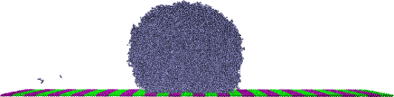
Figure 1: (Color Online) MD simulation snapshot of a static droplet at equilibrium. The droplet with $N=50000$ segments (iceblue) is on a striped surface having two types of atoms with $C_{s}=0.4$ (green) and $C_{s}=0.6$ (purple). The stripes have and equal widths of $w=7.56\sigma$.

A dissipative particle dynamics (DPD)Hoogerbrugge and Koelman (1992); Espanol and Warren (1995); Servantie and Müller (2008a) thermostat is used to keep the temperature of the system constant. The DPD thermostat has the advantage of conserving the momentum locally instead of globally as for the Nosé-Hoover thermostat. Hoogerbrugge and Koelman (1992); Espanol and Warren (1995); Soddemann, Dünweg, and Kremer (2003) The damping coefficient of the thermostat is set to $\gamma=0.5\tau^{-1}$ in all our simulations.

III Results

III.1 Equilibrium wetting properties

We calculate the equilibrium contact angles, $\theta_{E}$, of droplets for various strengths of the hydrophobicity parameter, $C_{s}$, and droplet sizes, $N$. We focus on cylindrical droplets in order to study larger liquid systems and have better statistics. We use droplet sizes from $N=10000$ to $N=50000$ monomers and hydrophobicity parameters in the range $C_{s}=0.3-0.8$ to study the equilibrium density profiles. The density profiles are obtained by counting the number of monomers in two-dimensional boxes of size $0.1\sigma$ in the $x$ and $z$ directions. We choose the contour line as the arithmetic mean of the densities of the polymer melt and its vapor, since the density of the vapor is negligible, the contour line corresponds to a density of $\rho_{p}/2=0.394\sigma^{-3}$. We depict in Fig.2 the density profiles for increasing number of monomers with the hydrophilic parameter set to $C_{s}=0.5$.

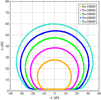
Figure 2: Density profiles for increasing monomer sizes $N=10000,\;20000,\;30000,\;40000,\;50000$. The surface is homogeneous with hydrophobic parameter $C_{s}=0.5$. The averaged equilibrium contact angle of these droplets is $\theta_{E}=137\degree\pm 1\degree$.

The contact angle is independent of the size of the droplet, we can hence evaluate the angle precisely by using drops of different sizes. Servantie and Müller (2008a) The geometry of cylindrical droplets at equilibrium satisfy the following relationships,

$$V = \frac{R^{2}}{2}\left(2\theta_{E}-\sin 2\theta_{E}\right)L_{y}$$ (4)

$$A = 2R\sin\theta_{E}Ly$$ (5)

$$H = R(1-\cos\theta_{E})$$ (6)

$$r_{z} = R\left(\frac{4}{3}\frac{\sin^{3}\theta_{E}}{2\theta_{E}-\sin 2\theta_{E}}-\cos\theta_{E}\right){}$$ (7)

where $V$, $H$, $A$, and $r_{z}$ are respectively the volume, the height, the area of contact with the substrate, and height of the center of mass. One can easily find the heights, $r_{z}$. Then, using the contour plots in Fig.2 we fit circles to the droplets to find the radius of the droplet $R$. One can then solve Eq. (7) numerically for $\theta_{E}$. The same procedure is applied for varying hydrophilic parameters. We depict in Fig. 3 the density profile of a droplet of $N=30000$ monomers for increasing values of $C_{s}$. As expected, increasing the strength of the attractive part of the interaction potential results in a more hydrophilic surface, and thus a lower contact angle. The inset of Fig.3 depicts the equilibrium contact angle as a function of $C_{s}$.

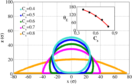
Figure 3: (Color online) Density profiles of droplets with $N=30000$ atoms for increasing hydrophilic parameters $C_{s}=0.4,\;0.5,\;0.6,\;0.7,\;0.8$. The surfaces are chemically homogeneous substrates. The inset represents the equilibrium contact angle as a function of the substrate strength.

We now focus on the striped surfaces. We determine from the inset of Fig. 3 that $C_{s}=0.4$ ($\theta_{E}=159\degree$) corresponds to a super-hydrophobic surface while $C_{s}=0.6$ ($\theta_{E}=110\degree$) is more hydrophilic. We choose those two values for the striped surfaces. We compute the equilibrium density profile of a droplet of $N=50000$ atoms on surfaces of varying stripe width from $w=1.26,\;2.52,\;3.78,\;5.04,\;6.30,\;7.56,\;8.82,\;10.08,\;11.34\sigma$. These values correspond to the stripe width to droplet length ratios of $w_{p}=3,\;5,\;8,\;10,\;13,\;15,\;18,\;20,\;23\%$. We depict in Fig. 4 the density profiles.

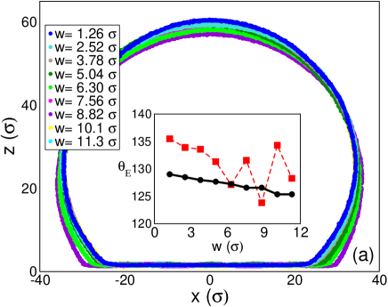
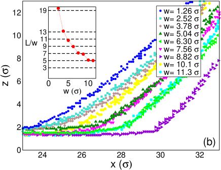
Figure 4: (Color online) (a) Density contours of a droplet of $N=50000$ atoms on different striped substrates. The circles in the inset represent the Cassie-Baxter angle, and the squares the actual equilibrium contact angle as a function of the stripe width $w$. (b) Close up view of the contact line for the different droplets, the inset depicts the length of the droplet divided by the stripe width $w$ as a function of $w$.

The inset of Fig. 4 (a) represents the equilibrium contact angles, and the contact angle corresponding to the Cassie-Baxter equation as a function of the stripe width. The Cassie-Baxter equation, Cassie and Baxter (1944) is a continuum result, it predicts the equilibrium contact angle of a droplet on a mixed surface as,

$$\cos\theta_{CB}=f_{1}\cos\theta_{1}+f_{2}\cos\theta_{2},$$ (8)

where $f_{1}$ and $f_{2}$ are respectively the contact area fractions of the surface of type 1 and 2, and $\theta_{1}$ and $\theta_{2}$ their respective equilibrium contact angles. We notice that, the calculated value $\theta_{E}$ is close to the continuum prediction $\theta_{CB}$. Indeed, on average we obtain $\theta_{E}=131\degree\pm 4\degree$ for the equilibrium contact angle, while the data for the homogeneous surfaces and $f_{1}=f_{2}=0.5$ yields $\theta_{CB}=127\pm 1\degree$. On the other hand, we notice that the contact angle decreases with the stripe width and varies wildly at large values of $w$. This is due to the fact that at equilibrium the droplet maximizes its contact area with the hydrophilic stripes in order to minimize the free energy. In order to achieve this the droplets slightly deforms to be in contact with one more hydrophilic stripe than hydrophobic stripes. In that case, the droplet has to be in contact with an odd number of stripes. As the stripe width increases, in order to accommodate an odd number of stripes, the droplet has to deform significantly, resulting in the important variation in the contact angle. We have depicted in Fig. 4(b) a close up on the contact line for all the different striped surfaces. In the inset we give the contact length to stripe width ratio. As we see, the length of the droplet varies as an odd number times the stripe width. In general, the fact that there is an extra hydrophilic stripe with respect to the hydrophobic one will make the surface effectively more hydrophilic, and hence with a lower contact angle. As the stripe width increases, the effect becomes more important, thus the contact angle will decrease with $w$. We remark that we have taken this effect into account while evaluating the Cassie-Baxter contact angle in Fig. 4(a).

III.2 Boundary condition

Before considering the dynamics of droplets on the different surfaces one has to evaluate the boundary condition. Indeed, we showed previously that for microscopic droplets the presence of slip at the surface can significantly affect the dynamics of the droplets. Specifically, for small droplets and large contact angles the slipping on the surface becomes the dominating dissipation mechanism leading to an increased velocity. Servantie and Müller (2008a) In the presence of slippage at the boundary one can use the Navier slip boundary condition,Navier (1823)

$$\eta\frac{\partial v_{x}}{\partial z}\Big{|}_{z_{b}}=\lambda v_{b}$$ (9)

where $z_{b}$ is the position of the boundary, $\lambda$ a damping coefficient quantifying the friction at the surface, and $v_{b}$ the velocity of the fluid on the surface. The damping coefficient can be evaluated thanks to a Green-Kubo relationship, namely,Bocquet and Barrat (1993, 1994)

$$\lambda=\frac{1}{k_{B}TA}\int_{0}^{\infty}dt\ \left\langle F_{s}(t)F_{s}(0)\right\rangle$$ (10)

where $F_{s}$ is the tangential force exerted by the substrate on the fluid, and $A$ the area of contact. The slip length is then given as,

$$\delta=\frac{\eta}{\lambda}$$ (11)

In order to evaluate $\delta$ we confine a fluid with $N=50000$ monomers between two surfaces with $L_{x}=90.7\sigma$ and $L_{y}=18.9\sigma$. The distance between the surfaces is tuned in order to recover the bulk liquid density far from the walls. After an equilibration, we compute the total transverse force for $4\times 10^{6}$ time steps and evaluate its time auto-correlation. Finally the slip length is obtained thanks to Eqs. 10 and 11. We depict the results in Fig. 5.

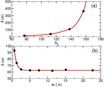
Figure 5: (Color online) (a) Slip length as a function of the equilibrium contact angle for homogeneous surfaces (b) Slip length as a function of the stripe width. The solid lines are guides for the eyes.

For homogeneous surfaces we notice a sharp increase of $\delta$ as a function of the equilibrium contact angle $\theta_{E}$. In each case, the slip length is important compared to the dimensions of the droplet, consequently we expect slippage to be the dominating mechanism of dissipation on the homogeneous surfaces. On the other hand, for the heterogeneous surfaces for very small widths we recover the value of $\delta$ corresponding to the homogeneous case i.e. for a contact angle of $\theta\approx 130\degree$ about $\delta\approx 90\ \sigma$, as the stripe width increases the slip length decreases and rapidly reaches a plateau at $\delta\approx 60\ \sigma$. The plateau is reached at approximately $3.5\ \sigma$, close to the effective size of the polymers. Indeed, the end-to-end distance of the polymers is found to be $R_{\rm ee}=3.447\ \sigma$. For very small stripe widths the stripes merge to an effective surface with an equilibrium contact angle corresponding to the Cassie-Baxter relation, as the stripe width increase the polymers interacts with the two distinct surfaces, leading to increased fluctuations at their boundaries, and consequently increased damping $\lambda$, therefore decreased slip length $\delta$. Once the stripes becomes larger than the polymers, the increased damping remains confined to the boundary between stripes, and thus a plateau is reached. We note that the slip length is important for both the homogeneous and heterogeneous surfaces, this is due to the fact that even though the striped surfaces are chemically heterogeneous they are still very smooth.

III.3 Dynamic wetting properties

In this section we focus on the dynamics of the cylindrical polymer droplets on the homogeneous and heterogeneous substrates. We first study homogeneous surfaces with only one type of atom. We consider three different hydrophilicity parameter $C_{s}=0.4,\;0.5,\;0.6$ which corresponds to the equilibrium contact angles $\theta_{E}=159\degree,\;137\degree\;,110\degree$. In order a to have a sustained motion we apply a bulk acceleration $a$ in the longitudinal direction $x$ to all the fluid atoms. The calculations are carried out for an equilibrated droplet of $N=50000$ monomers. We use five different values for the bulk acceleration, namely $a=0.00001,\;0.00002,\;0.00003,\;0.00004,\;0.00005$. After $2\times 10^{6}$ of equilibration steps, a non-equilibrium steady state is reached, we then compute the time average of the velocity of the center mass in the longitudinal direction, $\left\langle v_{\rm CM}\right\rangle$ for a further $2\times 10^{6}$ time steps. We depict the results in Fig.6.

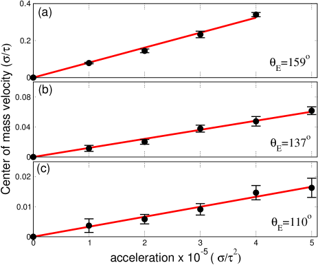
Figure 6: (Color online) x-component of the time-averaged velocity of the center of mass of the droplets for $N=50000$ monomers as a function of the acceleration for the chemically homogeneous surfaces with increasing wettability degrees, $(\text{\bf a})C_{s}=0.4,\;\theta_{E}=159\degree$, $(\text{\bf b})C_{s}=0.5,\;\theta_{E}=137\degree$, $(\text{\bf c})C_{s}=0.6,\;\theta_{E}=110\degree$. The circles are the results of the MD simulations and the plain lines are linear fits. The error bars correspond to the standard deviations of the means.

We showed previously Servantie and Müller (2008a) that the velocity profile in cylindrical droplets can be estimated by

$$v_{x}(z)=\frac{\rho_{p}}{\eta}\left[\left(H-\frac{z}{2}\right)z+\delta z\right]\ a$$ (12)

thus, the velocity of the center of mass can then be written as,

$$v_{\rm CM}=\frac{\rho_{p}}{\eta}\left[\left(H-\frac{r_{z}}{2}\right)r_{z}+\delta H\right]\ a$$ (13)

where $H$ is the height of the droplet and $\delta$ the slip length. This relationship is valid as long as the droplet is not deformed i.e. at small velocities. We hence expect a linear increase of the velocity with the acceleration. One could hence model the velocity of the center of mass as,

$$m_{\rm CM}\ \frac{dv_{\rm CM}}{dt}=-\gamma\ v_{\rm CM}+m_{\rm CM}\ a$$ (14)

where the effective damping coefficient $\gamma$ comprises all the different types of dissipation present in the droplet, namely, viscous dissipation in the volume, frictional dissipation at the surface, and dissipation at the contact line. At the steady state the expectation value of the center of mass velocity can then be written as,

$$v_{\rm CM}=\frac{\rho_{p}V}{\gamma}a.$$ (15)

Performing linear fits on the data in Fig. 6 permits to evaluate the effective dissipation coefficient $\gamma$. We present the results of the fits, and the expected value of the damping coefficient according to Eq. 13 in Table 1.

Table 1: Molecular Dynamics simulation results for polymer drops of $N=50000$ atoms on chemically homogeneous surfaces for the three wettability degrees, $C_{s}$. $\gamma$ corresponds to the calculated effective damping coefficient and $\gamma_{\rm MD}$ the one actually measured during the simulation.

$C_{s}$	$\theta_{E}$	$r_{z}$ ($\sigma)$	$H$ ($\sigma)$	$\delta$ ($\sigma)$	$\gamma$   $(m/\tau)$	$\gamma_{\rm MD}$   $(m/\tau)$
0.4	159°	31	63	364	14	6
0.5	137°	27	58	108	45	41
0.6	110°	23	52	40	112	150

We notice that apart for $C_{s}=0.4$ Eq. 13 gives a relatively good approximation of the damping coefficient. Errors come from two different approximation; firstly Eq. 13 is valid only when the contact angle is not too large, indeed it was derived according to the lubrication approximation, secondly, in order to evaluate the slip length with Eq. 11 one needs the local viscosity i.e. the viscosity at the surface. It is known that the mobility of the fluid atoms is affected by the strength of the substrate and consequently the viscosity. Servantie and Müller (2008b)

We previously looked to the size dependence of the steady state velocity. Servantie and Müller (2008a) For small droplets the dominating dissipation mechanism is the friction at the surface, in that case $v_{\rm CM}\sim R$. On the other hand, for large droplets the dominating dissipation mechanism is viscous dissipation in the volume, then $v_{\rm CM}\sim R^{2}$. In general, the velocity increases with size. Unfortunately, one can not write a simple scaling law for the dependence on contact angle in Eq. 13. Instead, one can look to the velocity at the top of the droplet $z=H$,

$$v_{\rm top}=\frac{\rho_{p}a}{\eta}\ \left(\frac{H}{2}+\delta\right)H$$ (16)

For droplets of fixed volume one can then get two limiting cases. For small droplets or a large slip length compared to its height the velocity at the top scales as $v_{\rm top}\sim\delta H$. While for large droplets or a small slip length compared its size one has $v_{\rm top}\sim H^{2}$. Notice that the height of a cylindrical droplet can be expressed as,

$$H=\sqrt{\frac{2V}{L_{y}}}\frac{1-\cos\theta_{E}}{\sqrt{2\theta_{E}-\sin 2\theta_{E}}},$$ (17)

which is a monotonically increasing function of the contact angle. Thus the steady state velocity of the droplet increases with its contact angle. As the surface becomes more hydrophobic, the shape of droplet becomes more like a sphere, which reduces the viscous damping during the rolling motion.

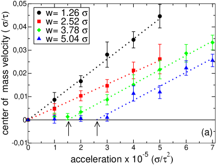
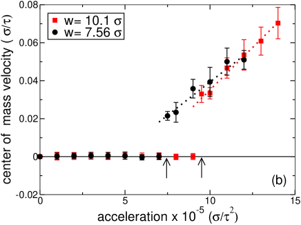
Figure 7: (Color online) Velocity of the center of mass of the droplets for $N=50000$ monomers as a function of the acceleration for the chemically heterogeneous surfaces. (a) $w=1.26-5.04\ \sigma$ and (b) $w=7.56\sigma$ and $w=10.1\ \sigma$. The symbols correspond to the results of the MD simulations and the dotted lines to linear fits. The error bars correspond to the standard deviations of the means. The arrows point to the depinning accelerations.

We now focus on the chemically heterogeneous substrate. We consider the liquid droplets in Fig. 4 and drive them with varying bulk accelerations $a$. Remark that we observed the contact angle hysteresis for $w_{p}\geq 23\%$ values, the results for these systems are not given in this paper. We depict the time averaged velocity of the center mass as a function of the acceleration for the different values of $w$ in Fig. 7. For the two smallest stripe widths, namely $w=1.26\ \sigma$ and $w=2.52\ \sigma$ the velocity of the center of mass is still a linear function of the acceleration. However, as the stripe width increase we notice that a minimum acceleration is required for a sustained motion, in other words the droplet remains pinned. Lets first focus on the pinned state. We notice that as the stripe width increases the minimum acceleration increases. Using the results in Fig. 7 we depict the critical acceleration in Fig. 8. We notice that apart for very small stripe widths, the depinning acceleration increases linearly with the stripe width. For small widths the energy barrier the droplet must cross is relatively small, consequently thermal fluctuations are enough to overcome it.

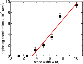
Figure 8: The minimum depinning force as a function of the stripe width $w$. The circles are the results from the MD simulations and the solid line a linear fit on the non-zero values of the depinning acceleration.

On the other hand, the linear increase of the depinning force can be explained easily by a qualitative argument. Indeed, when the droplet is pinned it maximizes its contact area with the hydrophilic stripes in order to minimize the free energy. One can see this effect clearly from the density fluctuations in pinned droplets in Fig. 9.

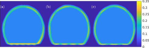
Figure 9: (Color online) Density fluctuations of a pinned droplet with a bulk acceleration $a=0.00001\;(\sigma/\tau^{2})$. (a) $w=5.04\ \sigma$, (b) $w=7.56\ \sigma$ and (c) $w=10.1\ \sigma$. The contour maps correspond to the standard deviation of the number density averaged over $2\times 10^{6}$ simulation time steps.

In order to maximize its contact with the hydrophilic stripes, each extremity of the droplet has to be on a hydrophilic stripe. In that case, if the droplet is in contact with $n$ hydrophobic stripes, it will be in contact with $n+1$ hydrophilic ones. Since there is slippage at the surface the whole contact area of the droplet moves instead of only the contact line. Assuming that $+W_{s}$ is the work required to move the fluid of a hydrophilic stripe to a hydrophobic one, then $-W_{s}$ is the work for the fluid moving from a hydrophobic stripe to a hydrophilic. Since there is an extra hydrophilic stripe there will remain a net work $+W_{s}$ in order to depin the droplet as schematized in Fig. 10.

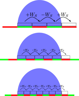
Figure 10: (Color online) An illustration for the depinning work $W_{s}$. A pinned droplet is in contact with $n$ hydrophobic stripes and $n+1$ hydrophilic stripes, the extremities must therefore be hydrophilic stripes.

The depinning work $W_{s}$ depends on the difference of surface energies $\Delta\gamma$ and on the area of fluid to move, thus $W_{s}\sim w\Delta\gamma$. If the temperature is large enough, $k_{B}T>W_{s}$, the thermal fluctuations are enough to depin the droplet. For lower temperatures, there will be a critical stripe width after which the droplet is pinned, and the depinning work will increase linearly with $w$.

We now focus on the dynamics of the droplet after the depinning. For the two smallest stripe width, we do not observe any pinning, and $\left\langle v_{\rm CM}\right\rangle$ increases linearly with the acceleration. Assuming the model for the homogeneous substrates is still valid, we perform linear fits on $\left\langle v_{\rm CM}\right\rangle$ and evaluate the effective damping coefficients. We give in Table 2 the results of the simulations and the value of $\gamma$ obtained from the slip lengths calculations and geometry of the droplet with Eqs. 13 and 15. Again we notice that the dynamics is relatively well described in terms of the model. For small stripe widths, the fact that the substrate is chemically heterogeneous does not alter significantly the dynamics. Except for a smaller slip length $\delta$, and thus a larger effective damping coefficient. This is due to the fact that while the surface is heterogeneous it is still smooth, the absence of surface roughness permits to slide and rotate easily on the substrate without any significant changes to the velocity profile inside the droplet.

Table 2: Molecular Dynamics simulation results for polymer drops of $N=50000$ atoms on chemically heterogeneous surfaces for different stripe widths.

$w(\sigma)$	$r_{z}\ (\sigma)$	$H\ (\sigma)$	$\delta\ (\sigma)$	$\gamma\;(m/\tau)$	$\gamma_{\rm MD}\;(m/\tau)$
1.26	27	59	74	60	56
2.52	27	58	64	68	96
3.78	27	59	62.5	68	81
5.04	26	57	62.5	71	83
7.56	26	57	62.5	71	71
10.08	27	58	62.5	71	57

Similarly, for the pinned droplets, after the critical acceleration, for large enough accelerations, we recover a linear regime for the velocity of the center of mass. We observe a sinusoidal variation of the velocity of the droplet as a function of time. As the edge of the droplet crosses from a hydrophilic stripe to a hydrophobic one, the total surface energy increases since the interaction is less attractive, and consequently, the kinetic energy increases. We have evaluated the average velocity and surface potential energy as a function of the position of the center of mass with respect to the substrate. We averaged the results over the distance of two stripes for better statistics, the results are depicted in Fig. 11(a) and Fig. 11(b) for the two largest stripes at an acceleration of $a=10^{-4}\ \sigma/\tau^{2}$ and for $w=3.78\ \sigma$ at $a=1.5\times 10^{-5}\ \sigma/\tau^{2}$.

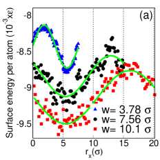
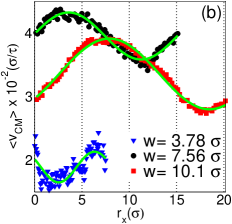
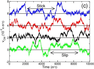
Figure 11: (Color online) (a) The surface energy per atom and (b) The averaged velocity of the center of mass as a function of the position of the center of mass. The plain lines correspond to sinusoidal fits. The center of mass velocity for $w=3.78\sigma$ is multiplied by 5 for better visualization. (c) Velocity of the center of mass as a function of time for four typical trajectories in the stick-slip regime, the velocity is translated.

When the surface energy is minimum, the center of mass of the droplet corresponds to the pinned position, in other words when it is in contact with one more hydrophilic stripe than a hydrophobic one. As the droplet crosses to a hydrophobic stripe its velocity decreases until it is in contact with one more hydrophobic stripe than a hydrophilic one, corresponding to the largest potential energy. Afterwards the velocity increases again. We notice that the modulation of the center of mass velocity does not affect significantly its mean value. Indeed, the linear fits in Fig. 7 and the corresponding results in Table 2 suggest that after the critical acceleration the dynamics of the droplet can still be relatively accurately described by the model.

On the other hand, one would expect that for accelerations just above the critical acceleration the dynamics would be consistent with stick-slip motion, in other words a succession of pinnings and depinnings. In that case, for a droplet in the pinned state, large thermal fluctuations allows to depin the droplet until it crosses to the next stripe and is pinned again. We do observe this behavior on individual trajectories as depicted in Fig. 11(c), however the time between depinnings varies wildly. Hence, once we consider time averages or the average on different trajectories one recovers the sinusoidal variation of the velocity as for the higher accelerations.

IV Conclusion

In this paper we presented coarsed-grained molecular dynamics simulation of the statics and dynamics of cylindrical polymer droplets on chemically homogeneous and heterogeneous surfaces. The surfaces consist of two layers of fcc lattices which interact with a modified Lennard-Jones potential with the polymeric fluid. The hydrophobicity of the surfaces is tuned with an empirical parameter weighting the attractive term. Chemically heterogeneous surfaces can then be defined with stripes of different hydrophobicity. We first evaluated the equilibrium contact angle on different surfaces. We showed that at equilibrium the droplet deforms slightly in order to accommodate one extra hydrophilic stripe with respect to hydrophobic ones. As a result, at equilibrium, the droplet has to be in contact with an odd number of stripes. As the stripe width increases this results in relatively large differences of contact angle. However, on average we have observed that the Cassie-Baxter relation gives a good approximation of the equilibrium contact angle.

We then focused on the boundary condition, indeed at microscopic scales the fluid can slip on the solid surface. This results in a combination of sliding and rotating motion for small droplets. We previously showed that on homogeneous surfaces, the steady-state velocity of the droplet scales linearly with the acceleration and depends only on its geometry i.e. contact angle and size, and the amount of slippage at the surface. Servantie and Müller (2008a) For small stripe widths, this is still true as the fluid only sees an effective surface, however, as the stripe width increases we noticed that the droplet becomes pinned until a sufficiently large acceleration is exerted. We showed that the depinning acceleration increases linearly with the stripe width. Since at equilibrium, the droplets extremities have to be on hydrophilic stripes, the net work required to depin the droplet is the work to move an amount of fluid from a hydrophilic stripe to an hydrophobic one, which in turn scales as the surface of the stripes. Once the droplet is depinned the steady-state velocity oscillates with time, consistent with the changes in surface energy when crossing different stripes. Finally, between the pinned state and linear regime we observed a characteristic stick-slip regime where large thermal fluctuations can depin the droplets.