Basis Expansions for Functional Snippets

Abstract

Estimation of mean and covariance functions is fundamental for functional data analysis. While this topic has been studied extensively in the literature, a key assumption is that there are enough data in the domain of interest to estimate both the mean and covariance functions. In this paper, we investigate mean and covariance estimation for functional snippets in which observations from a subject are available only in an interval of length strictly (and often much) shorter than the length of the whole interval of interest. For such a sampling plan, no data is available for direct estimation of the off-diagonal region of the covariance function. We tackle this challenge via a basis representation of the covariance function. The proposed approach allows one to consistently estimate an infinite-rank covariance function from functional snippets. We establish the convergence rates for the proposed estimators and illustrate their finite-sample performance via simulation studies and two data applications.

Keywords and phrases: Covariance estimation, Fourier series, Legendre polynomials, longitudinal data, penalized estimation, sequential compactness.

1 Introduction

Nowadays functional data are commonly encountered in practice, due to the advances in modern science and technology that enhance capability of data collection, storage and processing. Both unsupervised learning approaches, such as dimension reduction via functional principal component analysis (Rao, 1958; Dauxois et al., 1982; Hall and Hosseini-Nasab, 2009; Mas and Ruymgaart, 2015), and supervised learning, such as functional regression (Cardot et al., 1999; Müller and Stadtmüller, 2005; Ferraty and Vieu, 2006; Hall and Horowitz, 2007; Müller and Yao, 2008; Kong et al., 2016) are well studied in the literature. For a comprehensive treatment of these subjects, we recommend the monographs Ramsay and Silverman (2005), Ferraty and Vieu (2006), Horváth and Kokoszka (2012), Hsing and Eubank (2015) and Kokoszka and Reimherr (2017), and the review papers Wang et al. (2016) and Aneiros et al. (2019).

Critical to the statistical analysis of such data is the estimation of the mean and covariance functions, since they are the foundation of the aforementioned unsupervised and supervised learning tasks. For example, covariance estimation is a critical step to functional principal component analysis, as illustrated in Section 5. In addition, covariance estimation is often required for functional regression or classification for functional data. In reality, functions can only be recorded at a set of discrete points on the domain of the functions, where this set may vary among subjects and the measurements may contain noise. Estimation of mean and covariance functions in this context has been extensively studied by Rice and Silverman (1991), Cardot (2000), James et al. (2000), Cai and Yuan (2010), Cai and Yuan (2011), Yao et al. (2005b), Li and Hsing (2010) and Zhang and Wang (2016), among many others. In addition to the discrete nature of the observed functional data, subjects often stay in the study only for a subject-specific period that is much shorter than the span of the whole study. This usually does not cause much of a problem for mean estimation but brings challenges to covariance estimation.

For illustration and without loss of generality, we assume that the domain of the functional data $X(t)$ is the unit interval $\mathcal{T}=[0,1]$ and each subject only stays in the study for a period of length $\delta<1$. Data with these characteristics are termed “functional snippets”, in analogy to the longitudinal snippets analyzed in Dawson and Müller (2018). For such data, there is no information in the off-diagonal region $\mathcal{T}_{\delta}^{c}:=\{(s,t)\in[0,1]^{2}:|s-t|>\delta\}$ of the covariance function Cov$(X(s),X(t))$, and therefore there is no local information available for estimating the covariance function in this region. Mathematically, this amounts to

$$\mathbb{P}\{(\cup_{i=1}^{n}[A_{i},B_{i}]^{2})\cap\mathcal{T}_{\delta}^{c}=\emptyset\}=1,$$ (1)

for some $\delta>0$ and for all $n$, where $[A_{i},B_{i}]$ denotes the subinterval on which $X_{i}$ is observed. Figure 6(a) illustrates such a situation for the bone mineral density data, where the band with available data is prominent and narrow. Another example for a wider band is illustrated in Figure 9(a) for the systolic blood pressure data. Both data will be further studied in Section 5. For this type of data, local smoothing methods, e.g., the aforementioned Yao et al. (2005a) and Li and Hsing (2010), fail to yield a consistent estimate of the covariance function in the off-diagonal region as they are primarily interpolation methods.

The literature of statistical analysis for functional snippets is in its infancy. Delaigle and Hall (2016) proposed to approximate snippets by segments of Markov chains. This method is only valid at the discrete level, as shown by Descary and Panaretos (2019). More recently, to analyze functional snippets, Zhang and Chen (2018) and Descary and Panaretos (2019) used matrix completion techniques that innately work on a common grid of the domain $\mathcal{T}$. These approaches require modification when snippets are recorded on random and irregular design points, which is often encountered in applications. Yet, published theoretical analyses focus on the regular and dense design.

Another challenge is that estimating the covariance function for functional snippets is an extrapolation problem, which requires additional assumptions to overcome. The minimal identifiability condition for functional snippets is the trivial condition that the covariance function in the observable band $\mathcal{T}_{\delta}$ determines the covariance function on the entire domain. This minimal identifiability is a high-level concept (Delaigle et al., 2020), and consequently, existing works attempt to find some specialized conditions that imply the above minimal identifiability assumption. For instance, Descary and Panaretos (2019) assumed that the covariance function is an analytic function, and Delaigle et al. (2020) proposed the linear predictability assumption, which assumes that the values of the process $X(t)$ on a subinterval can be linearly predicted by the values of the same process on another subinterval.

In contrast to the aforementioned approaches, that impose a particular assumption on the process $X(t)$ itself or on its covariance function, we define identifiability through a family $\mathcal{C}$ in which the covariance function resides, and term such a family $\mathcal{T}_{\delta}$-identifiable if any two members from the family $\mathcal{C}$ and identical on the diagonal region $\mathcal{T}_{\delta}$ are equal everywhere. The $\mathcal{T}_{\delta}$-identifiability is the same as the above minimal identifiability except that we make the reference to a family explicit. The family $\mathcal{C}$ is comparable to the traditional parameter space or model, so our definition of identifiability is in line with the conventional statistical concept of identifiability that are imposed on the model. This concept of identifiability is rather general and encompasses the aforementioned identifiability assumptions as special cases. For example, the class of analytic functions considered in Descary and Panaretos (2019) and the class of covariance functions associated with linearly predictable random processes are $\mathcal{T}_{\delta}$-identifiable families; see Examples 1 and 4 for details. The primary reason that we adopt this minimal identifiability is that, our method and theory to be developed in Sections 2 and 3 apply to all $\mathcal{T}_{\delta}$-identifiable families under some regularity conditions.

Like functional snippets, fragments are also partially observed functional data and have been explored by many, such as Liebl (2013), Gellar et al. (2014), Goldberg et al. (2014), Kraus (2015), Gromenko et al. (2017), Stefanucci et al. (2018), Mojirsheibani and Shaw (2018), Kraus and Stefanucci (2019), Kneip and Liebl (2020) and Liebl and Rameseder (2019). However, the problem to recover the covariance function for functional fragments is often formulated as an interpolation problem, e.g., the work of Kneip and Liebl (2020) assumes that $\mathbb{P}([A_{i},B_{i}]^{2}=[0,1]^{2})>0$, which implies information and design points for the off-diagonal region $\mathcal{T}_{\delta}^{c}$ are still available. In contrast, information for that region is completely missing in the context of functional snippets (1), which significantly elevates the difficulty of statistical analysis. For this reason, we adopt the term functional snippets to distinguish them from fragments or other partially observed functional data.

Under the umbrella of $\mathcal{T}_{\delta}$-identifiability, we propose to approach functional snippets from the perspective of basis expansion. The main idea is to represent the covariance function by basis functions composed from tensor products of analytic orthonormal functions defined on $\mathcal{T}$. Basis functions, in particular spline basis functions, have been extensively explored in both nonparametric smoothing and functional data analysis by Wahba (1990), Wood (2003), Rice and Wu (2001), Ramsay and Silverman (2005) and Crambes et al. (2009), among many others. However, they are not suited for the extrapolation problem of functional snippets, as these bases are local. Unlike spline bases that are controlled by knots, analytic bases are global, in the sense that they are independent of local information such as knots or design points and are completely determined by their values on a countably infinite subset of the interval $\mathcal{T}$. This feature of analytic bases allows information to pass from the diagonal region to the off-diagonal region along the basis functions. Consequently, the missing pieces of the covariance function can then be inferred from the data available in the diagonal region when the covariance function is from a $\mathcal{T}_{\delta}$-identifiable class. In contrast, this is generally impossible for B-spline or other local bases.

In addition to the minimal identifiability assumption, the consistency of the proposed estimation method requires regularity conditions to overcome the challenges of extrapolation. One regularity condition that we identified is the bounded sequential compactness (BSC) of the family $\mathcal{C}$ of covariance functions under consideration. This new concept, developed in Section 3.3, essentially controls the complexity (or size) of the family $\mathcal{C}$ and enables us to establish the consistency and convergence rate of the proposed estimator in a nonparametric extrapolation setting. This condition is mild; for example, all families of functions that are uniformly bounded and Lipschitz continuous with a common Lipschitz constant are BSC families, as shown in Section 3.3. Such a regularity condition, not seen in the literature, is not required for interpolation and thus intrinsically separates nonparametric extrapolation from interpolation.

When our work was completed, we became aware of a related work that is independently developed by Delaigle et al. (2020). Although the work also uses a basis expansion approach, it is substantially different from ours. First, it focuses more on development of identifiability conditions while ours is on methodological development and theoretical analysis of the proposed estimators. Second, the method of Delaigle et al. (2020) extrapolates a pilot estimate from the diagonal region to the entire region by basis expansion without regularization. This may lead to excessive variability of the estimator in the off-diagonal region. In contrast, our method estimates the basis coefficients directly from data with penalized least squares and does not require a pilot estimate. Third, the convergence rate established in that work hinges on and thus is limited by the convergence rate of the pilot estimate, while our analysis gives an explicit rate that is adaptive to the smoothness of the underlying covariance function. Finally, the work of Delaigle et al. (2020) heuristically includes the identity function $f(x)=x$ into the Fourier basis to handle nonperiodicity, while ours adopts the Fourier extension technique that is well established in the field of numerical analysis.

In summary, this paper makes the following contributions to the field of functional snippet analysis. First, we develop a computationally efficient estimator for the covariance function based on basis expansion under the minimal identifiability condition. Second, we propose the novel concept of bounded sequential compactness, based on which we establish an explicit and adaptive rate of convergence for the proposed estimator without relying on any specific assumptions for identifibility. Such concept is new in the literature of nonparametric regression. Third, we introduce the well established numerical techniques, Fourier extension and geometric Newton method, to the field of functional data analysis for the first time.

2 Methodology

Let $\{X(t):t\in\mathcal{T}\}$ be a second-order stochastic process on a compact interval $\mathcal{T}\subset\mathbb{R}$, which without loss of generality is taken to be $[0,1]$. The mean and covariance functions of $X$ are defined as $\mu_{0}(t)=\mathbb{E}X(t)$ and $\gamma_{0}(s,t)=\text{Cov}(X(s),X(t)),$ respectively. The observed functions $X_{1},\ldots,X_{n}$ are statistically modeled as independent and identically distributed realizations of $X$. In practice, each realization $X_{i}$ is only recorded at subject-specific $m_{i}$ time points $T_{i1},\ldots,T_{im_{i}}$ with measurement errors. More precisely, for functional snippets, the observed data are pairs $(T_{ij},Y_{ij})$, where

$$Y_{ij}=X_{i}(T_{ij})+\varepsilon_{ij},\quad i=1,\ldots,n,\quad j=1,\ldots,m_{i},$$ (2)

$\varepsilon_{ij}$ is the random noise with mean zero and unknown variance $\sigma^{2}$, and there is a $\delta\in(0,1)$ for which $|T_{ij}-T_{ik}|\leq\delta$ for all $i$, $j$ and $k$. The focus of this paper is to estimate the mean and covariance functions of $X$ using these data pairs $(T_{ij},Y_{ij})$.

2.1 Mean Function

Although functional snippets pose a challenge for covariance estimation, they usually do not obstruct mean estimation, since data for the estimation are available likely across the whole domain of interest. In light of this observation, traditional methods such as local linear smoothing (Yao et al., 2005b; Li and Hsing, 2010) can be employed. Below we adopt an analytic basis expansion approach. The advantage of this approach is its computational efficiency and adaptivity to the regularity of the underlying mean function $\mu_{0}$; see also Section 3.2.

Let $\boldsymbol{\Phi}=\{\phi_{1},\ldots\}$ be a complete orthonormal basis of $L^{2}(0,1)$ that consists of squared integrable functions defined on the interval $[0,1]$. When $\mu_{0}\in L^{2}(0,1)$, it can be represented by the following series in terms of the basis $\boldsymbol{\Phi}$,

$$\mu_{0}(t)=\sum_{k=1}^{\infty}a_{k}\phi_{k}(t),$$

where $a_{k}=\int_{0}^{1}\mu_{0}(t)\phi_{k}(t)\mathrm{d}t$. In practice, one often approximates such series by its first $q>0$ leading terms, where $q$ is a tuning parameter controlling the approximation quality. The coefficients $a_{1},\ldots,a_{q}$ are then estimated from data by penalized least squares. Specifically, with the notation $\boldsymbol{\Phi}_{q}(t)=(\phi_{1}(t),\cdots,\phi_{q}(t))^{\top}\in\mathbb{R}^{q}$ and $\mathbf{a}_{0}=(a_{1},\ldots,a_{q})^{\top}$, the estimator of $\mathbf{a}_{0}=(a_{1},\ldots,a_{q})^{\top}$ is given by

$$\hat{\mathbf{a}}=\mathop{\arg\min}\limits_{\textbf{a}\in\mathbb{R}^{q}}\Big{\{}\sum_{i=1}^{n}v_{i}\sum_{j=1}^{m_{i}}[Y_{ij}-\textbf{a}^{\top}\boldsymbol{\Phi}_{q}(T_{ij})]^{2}+\rho H(\textbf{a}^{\top}\boldsymbol{\Phi}_{q})\Big{\}},$$ (3)

and $\mu_{0}$ is estimated by

$$\hat{\mu}(t)=\hat{\mathbf{a}}^{\top}\boldsymbol{\Phi}_{q}(t),$$

where the weights $v_{i}>0$ satisfy $\sum_{i=1}^{n}v_{i}m_{i}=1$, $H(\cdot)$ represents the roughness penalty, and $\rho$ is a tuning parameter that provides trade-off between the fidelity to the data and the smoothness of the estimate. There are two commonly used schemes for the weights, equal weight per observation (OBS) and equal weight per subject (SUBJ), for which the weights $v_{i}$ are $1/(\sum_{i=1}^{n}m_{i})$ and $1/(nm_{i})$, respectively. These and also alternative weight schemes are discussed in Zhang and Wang (2016, 2018).

The penalty term in (3) is introduced to prevent excessive variability of the estimator when a large number of basis functions are required to adequately approximate $\mu_{0}$ and when the sample size is not sufficiently large. In the asymptotic analysis of $\hat{\mu}$ in Section 3, we will see that this penalty term does not affect the convergence rate of $\hat{\mu}$ when the tuning parameter $\rho$ is not too large. In our study, the roughness penalty is given by

$$H(g)=\int_{0}^{1}\{g^{(2)}(t)\}^{2}\mathrm{d}t,$$

where $g^{(2)}$ denotes the second derivative of $g$. In matrix form, for $g(t)=\mathbf{a}^{\top}\boldsymbol{\Phi}_{q}(t)$, it equals $\textbf{a}^{\top}\textbf{W}\textbf{a}$, where $\mathbf{W}$ is a $q\times q$ matrix with elements $W_{kl}=\int_{0}^{1}\phi_{k}^{(2)}(t)\phi_{l}^{(2)}(t)\mathrm{d}t$. The choices of $q$ and $\rho$ are discussed in Section 4.1.

2.2 Covariance Function

Since functional snippets do not provide any direct information for the off-diagonal region, the only way to recover the covariance in the off-diagonal region is to infer it from the diagonal region. The following definition formulates this basic requirement for identifiability.

Definition 1.

A family $\mathcal{C}$ of covariance functions is called a $\mathcal{T}_{\delta}$-identifiable family if $\gamma_{1},\gamma_{2}\in\mathcal{C}$ and $\gamma_{1}(s,t)=\gamma_{2}(s,t)$ for all $(s,t)\in\mathcal{T}_{\delta}$ imply that $\gamma_{1}(s,t)=\gamma_{2}(s,t)$ for all $(s,t)\in\mathcal{T}^{2}$.

Intuitively, we consider a family $\mathcal{C}$ of covariance functions and require the covariance functions to be uniquely identified within the family $\mathcal{C}$ by their values on the diagonal region. Below we provide four examples to illustrate the ubiquitousness of $\mathcal{T}_{\delta}$-identifiable families.

Example 1 (Analytic functions).

A function is analytic if it can be locally represented by a convergent power series. According to Corollary 1.2.7 of Krantz and Parks (2002), if two analytic functions agree on $\mathcal{T}_{\delta}$, then they are identical on $[0,1]^{2}$. Thus, the family of analytic functions is a $\mathcal{T}_{\delta}$-identifiable family as observed by Descary and Panaretos (2019), who also provided an elegant counterexample to demonstrate that $C^{\infty}([0,1]^{2})$, the space of infinitely differentiable functions, is not $\mathcal{T}_{\delta}$-identifiable.

Example 2 (Sobolev sandwich families).

For any $0<\epsilon<\delta$, consider the family of continuous functions that belong to a two-dimensional Sobolev space on $\mathcal{T}_{\epsilon}$ and are analytic elsewhere. Such functions have an $r$-times differentiable diagonal component sandwiched between two analytic off-diagonal pieces. The family is $\mathcal{T}_{\delta}$-identifiable, because the values of such functions on the off-diagonal region are fully determined by the values on the uncountable set $\mathcal{T}_{\epsilon}^{c}\cap\mathcal{T}_{\delta}\subset\mathcal{T}_{\delta}$ according to Corollary 1.2.7 of Krantz and Parks (2002). Note that this family contains functions with derivatives only up to a finite order.

Example 3 (Semiparametric families).

Consider the family of functions of the form $g(s)h(s,t)g(t)$, where $g$ is a function from a nonparametric class $\mathcal{G}$ and $h$ is from a parametric class $\mathcal{H}$ of correlation functions. This family, considered in Lin and Wang (2020), is generally $\mathcal{T}_{\delta}$-identifiable, as long as both $\mathcal{G}$ and $\mathcal{H}$ are identifiable. For instance, when $\mathcal{G}$ is a one-dimensional Sobolev space and $\mathcal{H}$ is the class of Matérn correlation functions, the family is $\mathcal{T}_{\delta}$-identifiable. Note that no analyticity is assumed for this family.

Example 4 (Linearly predictable families).

For a random process $X$ defined on $\mathcal{T}$, we say that the snippet $\{X(t)\}_{t\in I^{\ast}}$ on the subinterval $I^{\ast}\subset\mathcal{T}$ is linearly $(B,\epsilon)$-predictable (Delaigle et al., 2020) from another subinterval $I\subset\mathcal{T}$, if for all $t\in I^{\ast}$, there exists an integrable function $L_{t}(s)$ defined on $I$ such that $\sup_{t\in I^{\ast}}\sup_{s\in I}|L_{t}(s)|<\infty$, $\sup_{t\in I^{\ast}}\int_{I}|L_{t}(s)|\mathrm{d}s<{B}$ and $X(t)=\mu(t)+\int_{I}L_{t}(s)\{X(s)-\mu(s)\}\mathrm{d}s+Z(t)$, where for all $t\in I^{\ast}$, $Z(t)$ is a zero mean random variable such that $\mathbb{E}Z^{2}(t)\leq\epsilon^{2}$. Fix an integer $h>0$ and a partition $I_{0},\ldots,I_{h}$ of $\mathcal{T}$ such that $I_{j}\times I_{j}\subset\mathcal{T}_{\delta}$. Consider only the class $\mathscr{X}$ of random processes $X$ whose snippet $\{X(t)\}_{t\in I_{j}}$ is linearly $(B_{j},\epsilon_{j})$-predictable from $I_{j^{\ast}}$ for some $0\leq j^{\ast}\leq j-1$ and all $\epsilon_{j}>0$, and for all $j=1,\ldots,h$. Let $\mathcal{L}$ be the collection of covariance functions of random processes in $\mathscr{X}$. By Delaigle et al. (2020), each member in $\mathcal{L}$ is identifiable within $\mathcal{L}$ from its values on the diagonal region $\mathcal{T}_{\delta}$, and thus $\mathcal{L}$ is $\mathcal{T}_{\delta}$-identifiable.

With the $\mathcal{T}_{\delta}$-identifiability of the family $\mathcal{C}$, it is now possible to infer the off-diagonal region by the information contained in the raw covariance $\Gamma_{ijk}=\{Y_{ij}-\hat{\mu}(T_{ij})\}\{Y_{ik}-\hat{\mu}(T_{ik})\}$ available only in the diagonal region. To this end, we propose to transport information from the diagonal region to the off-diagonal region through the basis functions $\phi_{k}\otimes\phi_{l}$ with $(\phi_{k}\otimes\phi_{l})(s,t)=\phi_{k}(s)\phi_{l}(t)$ for $s,t\in\mathcal{T}$, by approximating $\gamma_{0}$ with

$$\gamma_{{\mathbf{C}}_{0}}(s,t)=\sum_{1\leq k,l\leq p}c_{kl}\phi_{k}(s)\varphi_{l}(t),\quad(s,t)\in[0,1]^{2},$$ (4)

where $c_{kl}=\iint\gamma_{0}(s,t)\phi_{k}(s)\phi_{l}(t)\mathrm{d}s\mathrm{d}t$, ${\mathbf{C}}_{0}$ is the matrix of coefficients $c_{kl}$, and $p\geq 1$ is an integer. There are countless bases that can serve in (4); however, if we choose an analytic basis $\boldsymbol{\Phi}$, then their values in the diagonal region completely determine their values in the off-diagonal region. When such a representation of the covariance function $\gamma_{0}$ is adopted and the unknown coefficients $c_{kl}$ are estimated from data, the information contained in the estimated coefficients extends from the diagonal region to the off-diagonal region through the analyticity of the basis functions.

To estimate the coefficients $c_{kl}$ from data, we adopt the idea of penalized least squares, where the squared loss of a given function $\gamma$ is measured by the sum of weighted squared errors

$$SSE(\gamma)=\sum_{i=1}^{n}w_{i}\sum_{1\leq j\neq k\leq m_{i}}\{\Gamma_{ijl}-\gamma(T_{ij},T_{il})\}^{2},$$

where $w_{i}>0$ are weights satisfying $\sum_{i=1}^{n}m_{i}(m_{i}-1)w_{i}=1$, while the roughness penalty is given by

$$J(\gamma)=\iint\frac{1}{2}\left\{\left[\frac{\partial^{2}\gamma}{\partial s^{2}}\right]^{2}+2\left[\frac{\partial^{2}\gamma}{\partial s\partial t}\right]^{2}+\left[\frac{\partial^{2}\gamma}{\partial t^{2}}\right]^{2}\right\}\mathrm{d}s\mathrm{d}t.$$

Then,

$${J}(\gamma_{\mathbf{C}})=\mathrm{tr}(\textbf{C}\textbf{U}\textbf{C}\textbf{W})+\mathrm{tr}(\textbf{C}\textbf{V}\textbf{C}\textbf{V}),$$ (5)

where $\gamma_{\mathbf{C}}$ is defined in (4) with ${\mathbf{C}}_{0}$ replaced by $\mathbf{C}$, $\mathrm{tr}$ denotes the matrix trace, and $\mathbf{U},\mathbf{V}$ are $p\times p$ matrices with elements $U_{kl}=\int_{0}^{1}\phi_{k}(s)\phi_{l}(s)\mathrm{d}s$ and $V_{kl}=\int_{0}^{1}\phi_{k}^{(1)}(s)\phi_{l}^{(1)}(s)\mathrm{d}s$, respectively. The estimator $\hat{\gamma}(s,t)$ of $\gamma_{0}(s,t)$ is then taken as $\hat{\gamma}(s,t)=\boldsymbol{\Phi}_{p}^{\top}(s)\hat{\mathbf{C}}\boldsymbol{\Phi}_{p}(t)$ with

$$\hat{\mathbf{C}}=\mathop{\arg\min}\limits_{\mathbf{C}:\,\gamma_{\mathbf{C}}\in\mathcal{C}}\,\sum_{i=1}^{n}w_{i}\sum_{1\leq j\neq l\leq m_{i}}\{\Gamma_{ijl}-\gamma_{\textbf{C}}(T_{ij},T_{il})\}^{2}+\lambda{J}(\gamma_{\mathbf{C}}),$$ (6)

where $\lambda$ is a tuning parameter that provides a trade-off between the fidelity to the data and the smoothness of the estimate. Numerical method to solve the constraint optimization (6) is detailed in Appendix B.

Similar to (3), the penalty term in (6) is introduced to overcome excessive variability of an estimator when a large number of basis functions are required while the sample size is relatively small. It does not affect the convergence rate of $\hat{\gamma}$ when the tuning parameter $\lambda$ is not too large. The choices of $p$ and $\lambda$ are discussed in Section 4.1. For the choice of the weights $w_{i}$, Zhang and Wang (2016) discussed several weighing schemes, including the OBS scheme $w_{i}=1/\{\sum_{i=1}^{n}m_{i}(m_{i}-1)\}$ and the SUBJ scheme $w_{i}=1/\{nm_{i}(m_{i}-1)\}$. An optimal weighing scheme was proposed in Zhang and Wang (2018); we refer to this paper for further details.

3 Theory

As functional snippets are often sparsely recorded, in the sense that $m_{i}\leq m_{0}<\infty$ for all $i=1,\ldots,n$ and some $m_{0}>0$, in this section we focus on theoretical analysis tailored to this scenario. For simplicity, we assume that the number of observations for each trajectory is equal, i.e., $m_{i}=m$ for all $i=1,\ldots,n$. Note that under this assumption, the SUBJ and OBJ schemes coincide. The results for general number $m_{i}$ of observations and weight schemes can be derived in a similar fashion. We start with a discussion on the choice of basis functions and then proceed to study the convergence rates of the estimated mean and covariance functions.

3.1 Analytic Basis

While all complete orthonormal bases can be used for the proposed estimator in (3), an analytic basis is preferred for the estimator in (6). For a clean presentation, we exclusively consider analytic bases $\boldsymbol{\Phi}=\{\phi_{1},\ldots\}$ that work for both (3) and (6). In this paper, a basis is called an analytic $(\alpha,\beta)$-basis if its basis functions are all analytic and satisfy the following property: for some constants $\alpha,\beta\geq 0$, there exists a constant $C$ such that $\|\phi_{k}\|_{\infty}\leq Ck^{\alpha}$ and $\|\phi_{k}^{(r)}\|_{L^{2}}\leq Ck^{\beta r}$ for $r=1,2$ and all $k=1,\ldots$. Here, $\|\phi_{k}\|_{\infty}$ denotes the supremum norm of $\phi_{k}$, defined by $\sup_{t\in[0,1]}|\phi_{k}(t)|$, and $\phi_{k}^{(r)}$ represents the $r$th derivative of $\phi_{k}$. Throughout this paper, we assume that the basis $\boldsymbol{\Phi}=\{\phi_{1},\ldots\}$ is an analytic $(\alpha,\beta)$-basis.

Different bases lead to different convergence rates of the approximation to $\mu_{0}$ and $\gamma_{0}$. For the mean function $\mu_{0}$, when using the first $q$ basis functions $\phi_{1},\ldots,\phi_{q}$, the approximation error is quantified by

$$\mathcal{E}(\mu_{0},\boldsymbol{\Phi},q)=\left\|\mu_{0}-\sum_{k=1}^{q}a_{k}\phi_{k}\right\|_{L^{2}},$$

where we recall that $a_{k}=\int_{0}^{1}\mu_{0}(t)\phi_{k}(t)\mathrm{d}t$. The convergence rate of the error $\mathcal{E}(\mu_{0},\boldsymbol{\Phi},q)$, denoted by $\tau_{q}=\tau_{q}(\mu_{0},\boldsymbol{\Phi})$, signifies the approximation power of the basis $\boldsymbol{\Phi}$ for $\mu_{0}$. Similarly, the approximation error for $\gamma_{0}$ is measured by

$$\mathcal{E}(\gamma_{0},\boldsymbol{\Phi},p)=\left\|\gamma_{0}-\sum_{k=1}^{p}\sum_{l=1}^{p}c_{kl}\phi_{k}\otimes\phi_{l}\right\|_{L^{2}},$$

where the $L^{2}$ norm of a function $\gamma(s,t)$ is defined by $\|\gamma\|_{L^{2}}=\{\int_{0}^{1}\int_{0}^{1}|\gamma(s,t)|^{2}\mathrm{d}s\mathrm{d}t\}^{1/2}$. The convergence rate of $\mathcal{E}(\gamma_{0},\boldsymbol{\Phi},p)$ is denoted by $\kappa_{p}=\kappa_{p}(\gamma_{0},\boldsymbol{\Phi})$. Below we discuss two examples of bases.

Example 5 (Fourier basis).

Fourier basis functions, defined by $\phi_{1}(t)=1$, $\phi_{2k}(t)=\cos(2k\pi t)$ and $\phi_{2k+1}(t)=\sin(2k\pi t)$ for $k\geq 1$, constitute a complete orthonormal basis of $L^{2}(\mathcal{T})$ for $\mathcal{T}=[0,1]$. It is also an analytic $(0,1)$-basis. When $\mu_{0}$ is periodic on $\mathcal{T}$ and belongs to the Sobolev space $\mathscr{H}^{r}(\mathcal{T})$ (see Appendix A.11.a and A.11.d of Canuto et al. (2006) for the definition), then, according to Eq. (5.8.4) of Canuto et al. (2006) one has $\tau_{q}=O(q^{-r})$. Similarly, if $\gamma_{0}$ is periodic and belongs to $\mathscr{H}^{r}(\mathcal{T}^{2})$, then $\kappa_{p}=O(p^{-r})$. When $\mu_{0}$ or $\gamma_{0}$ is not a periodic function, a technique called Fourier extension, briefly described in Appendix A, can be adopted to yield the same rate (Adcock et al., 2014). This technique is well studied in the field of computational physics (Boyd, 2002) and numerical analysis (Huybrechs, 2010) as a tool to overcome the so-called Gibbs phenomenon (Zygmund, 2003), but seems not well explored in statistics yet. In Section 4, we numerically illustrate the application of this technique.

Example 6 (Legendre polynomials).

The canonical Legendre polynomial $P_{k}(t)$ of degree $k$ is defined on $[-1,1]$ by

$$P_{k}(t)=\frac{1}{2^{k}k!}\frac{\mathrm{d}^{k}}{\mathrm{d}t^{k}}\{(x^{2}-1)^{k}\}.$$

These polynomials are orthogonal in $L^{2}(-1,1)$. By a change of variable and normalization, they can be turned into an orthonormal basis of $L^{2}(\mathcal{T})$. The Legendre polynomials have numerous applications in approximation theory and numerical integration; see Wang and Xiang (2011) and references therein. One can show that the Legendre basis is an analytic $(1/2,1)$-basis. According to Eq (5.8.11) of Canuto et al. (2006), one has $\tau_{q}=O(q^{-r})$ and $\kappa_{p}=O(p^{-r})$ when $\mu_{0}$ belongs to $\mathscr{H}^{r}(\mathcal{T})$ and $\gamma_{0}$ belongs to $\mathscr{H}^{r}(\mathcal{T}^{2})$, respectively.

3.2 Mean function

For functional snippets, we shall assume that the observations from a subject scatter randomly in a subject specific time interval, whose length is $\delta$ and whose middle point is called the reference time in this paper. We further assume that the reference time $R_{i}$ of the $i$th subject are independently and identically distributed in the interval $[\delta/2,1-\delta/2]$, and the observed time points $T_{i1},\ldots,T_{im_{i}}$, conditional on $R_{i}$, are independently and identically distributed in the interval $[R_{i}-\delta/2,R_{i}+\delta/2]$.

To study the estimator $\hat{\mu}$, we make the following assumptions.

A.1

There exist $0<\mathfrak{c}_{1}\leq\mathfrak{c}_{2}<\infty,$ such that the density $f_{R}(s)$ of the reference time $R$ satisfies $\mathfrak{c}_{1}\leq f_{R}(s)\leq\mathfrak{c}_{2},$ for any $s\in[\delta/2,1-\delta/2]$. There exist $0<\mathfrak{c}_{3}\leq\mathfrak{c}_{4}<\infty$, such that the conditional density $f_{T|R}(t|s)$ of the observed time $T$ satisfies $\mathfrak{c}_{3}\leq f_{T|R}(t|s)\leq\mathfrak{c}_{4}$, for any given reference time $s\in[\delta/2,1-\delta/2]$ and $t\in[s-\delta/2,s+\delta/2]$.

A.2

$\mathbb{E}\|X\|_{L^{2}}^{2}\leq\mathfrak{c}_{5}<\infty$ for some constant $\mathfrak{c}_{5}>0$.

A.3

$q^{2\alpha+2}/n\rightarrow 0$ and $\rho/(n^{-1/2}q^{\alpha-4\beta-1/2})\rightarrow 0$.

Assumption A.1 requires the density of the reference time and conditional densities of the time points to be bounded away from zero and infinity. This also guarantees that the marginal probability density of the time points $T_{ij}$ is bounded away from zero and infinity. Assumption A.2 is mild and assumption A.3 facilitates the convergence rate, where the dimension $q$ can grow with $n$. In the sequel, we use $a_{n}\asymp b_{n}$ to denote $0<\lim_{n\rightarrow\infty}a_{n}/b_{n}<\infty$.

Theorem 1.

If $\boldsymbol{\Phi}$ is a $(\alpha,\beta)$-basis, conditions (A.1)–(A.3) imply that

$$\|\hat{\mu}-\mu_{0}\|_{L^{2}}^{2}=O_{P}\Big{(}\frac{q^{2\alpha+1}}{n}+\tau_{q}^{2}\Big{)},$$ (7)

where $\tau_{q}$ is the convergence rate of $\mathcal{E}(\mu_{0},\boldsymbol{\Phi},q)$ defined in section 3.1.

We first note that, under condition A.3, the tuning parameter $\rho$ does not have direct impact on the asymptotic rate of $\hat{\mu}$. We also observe that in (7), the term $q^{2\alpha+1}n^{-1}$ specifies the estimation error using a finite sample, while $\tau_{q}$ is the deterministic approximation error for using only the first $q<\infty$ basis functions. The latter term depends on the smoothness of $\mu_{0}$. Intuitively, it is easier to approximate smooth functions with basis functions. For a given number of basis functions, smoother functions generally yield smaller approximation errors. As discussed in Example 5 and 6, when $\mu_{0}$ belongs to the Sobolev space $\mathscr{H}^{r}(0,1)$, i.e., $\mu_{0}$ is $r$ times differentiable, we have $\tau_{q}=O(q^{-r})$. This leads to the following convergence rate, using either the Fourier basis or the Legendre basis.

Corollary 1.

Suppose $\mu_{0}^{(r)}$ exists and satisfies $\|\mu_{0}^{(r)}\|_{L^{2}}<\infty$ for some $r\geq 1$. Assume conditions (A.1)–(A.3) hold.

1. If $\boldsymbol{\Phi}$ is the Fourier basis and $\mu_{0}$ is periodic, then $\|\hat{\mu}-\mu_{0}\|_{L^{2}}^{2}=O_{P}(n^{-2r/(2r+1)})$ with the choice $q\asymp n^{1/(2r+1)}$.

2. If $\boldsymbol{\Phi}$ is the Legendre basis, then $\|\hat{\mu}-\mu_{0}\|_{L^{2}}^{2}=O_{P}(n^{-r/(r+1)})$ with the choice $q\asymp n^{1/(2r+2)}$.

For $r=2$ and a periodic function $\mu_{0}$, the convergence rate for $\hat{\mu}$ is $n^{-2/5}$ and $n^{-1/3}$, respectively, for the estimator based on Fourier and Legendre bases. We can see that the convergence rate is faster for a Fourier basis. This is because, although they are both $(\alpha,\beta)$-bases, $\alpha=1/2$ for the Legendre basis is larger than $\alpha=0$ for the Fourier basis. According to (7), a larger value of $\alpha$ leads to a slower rate. Indeed, $\alpha$ controls the growth rate of the extrema of basis functions. Fourier basis functions are uniformly bounded between $-1$ and $1$. In contrast, high-order Legendre basis functions tend to have large extrema that amplify variability. This limits the number of basis functions for estimation and thus causes a slower convergence rate for the Legendre basis. When $\mu_{0}$ is nonperiodic, the classic Fourier basis suffers from the so-called Gibbs phenomenon which, however, can be substantially alleviated by the Fourier extension technique; see Section 4 and Appendix A for more details.

3.3 Covariance function

In Section 2 we assumed $\gamma_{0}$ to reside in a $\mathcal{T}_{\delta}$-identifiable family $\mathcal{C}$ in order to meet a basic criterion of identifiability. To study the asymptotic properties of the covariance estimator, we require the family $\mathcal{C}$ to satisfy an additional regularity condition as described below. Let $\mathcal{F}$ be the space of real-valued functions defined on $\mathcal{T}^{2}$ endowed with the product topology. In this topology, a sequence of functions $\{f_{k}\}$ converges to a limit $f$ if and only if

$$\lim\limits_{k\rightarrow\infty}f_{{k}}(s,t)=f(s,t),\quad\text{for\ all}\ (s,t)\in\mathcal{T}^{2}.$$

Definition 2.

A subset $\mathcal{S}$ of $\mathcal{F}$ is called a bounded sequentially compact (BSC) family if every sequence $\{f_{k}\}\subset\mathcal{S}$ that is bounded in the $L^{2}$ norm, i.e., $\sup_{k}\|f_{k}\|_{L^{2}}<\infty$, has a subsequence converging to a limit in $\mathcal{S}$ in the product topology.

The BSC concept is closely related to the topological concept “sequential compactness”. Specifically, a subset $\mathcal{S}\subset\mathcal{F}$ is sequentially compact if every sequence in $\mathcal{S}$ has a subsequence that converges to a limit in $\mathcal{S}$ in the topology of $\mathcal{F}$. In particular, sequential compactness is stronger than BSC and thus implies the latter. However, when the subset $\mathcal{S}$ is uniformly bounded in the $L^{2}$ norm, i.e., $\sup_{f\in\mathcal{S}}\|f\|_{L^{2}}<\infty$, then the two concepts coincide. If all functions in $\mathcal{S}$ are bounded by a common constant and are Lipschitz continuous with a common Lipschitz constant, then $\mathcal{S}$ is a BSC family. To see this, we note that such family is locally equicontinuous, and also the set $\{f(s,t):f\in\mathcal{S}\}$ is bounded for all $s,t\in\mathcal{T}$. Then the claim follows from the Arzelà–Ascoli Theorem (Chapter 7, Remmert, 1997). Also, the product of two BSC families of which the functions are uniformly bounded in the $L^{2}$ norm is also a BSC family. This property is useful for constructing new BSC families from existing ones; see Example 8 for an illustration. The following proposition, of which the proof is trivial or already discussed in the above and thus is omitted, summarizes the aforementioned properties of BSC and its connections to sequential compactness.

Proposition 1.

Let $\mathcal{F}$ be the collection of real-valued functions defined on $\mathcal{T}^{2}$ and endowed with the product topology. Let $\mathcal{S}$ be a subset of $\mathcal{F}$.

1. If $\mathcal{S}$ is sequentially compact, then it is a BSC family.

2. If $\mathcal{S}$ is a BSC family and $\sup_{f\in\mathcal{S}}\|f\|_{L^{2}}<\infty$, then $\mathcal{S}$ is sequentially compact.

3. If $\sup_{f\in\mathcal{S}}\|f\|_{\infty}<\infty$ and $\sup_{f\in\mathcal{S}}\sup_{x\neq y}|f(x)-f(y)|/\|x-y\|_{2}<\infty$, then $\mathcal{S}$ is a BSC family.

4. If both $\mathcal{S}$ and $\mathcal{Q}\subset\mathcal{F}$ are sequentially compact, then the family $\mathcal{S}\mathcal{Q}=\{fg:f\in\mathcal{S},g\in\mathcal{Q}\}$ is also sequentially compact. Consequently, if $\mathcal{S}$ and $\mathcal{Q}$ are BSC families satisfying $\sup_{f\in\mathcal{S}\cup\mathcal{Q}}\|f\|_{L^{2}}<\infty$, then $\mathcal{S}\mathcal{Q}$ is also a BSC family.

The following examples utilize Proposition 1 to exhibit BSC families and illustrate the abundance of BSC families.

Example 7 (Bounded Sobolev sandwich families).

Let $M_{1},M_{2}>0$ be fixed but potentially arbitrarily large constants. Let $\mathcal{S}(M_{1},M_{2})$ be the subfamily of the $\mathcal{T}_{\delta}$-identifiable family introduced in Example 2 such that, if $f\in\mathcal{S}(M_{1},M_{2})$ then $\|f\|_{\infty}\leq M_{1}$ and the Lipschitz constant of $f$ is bounded by $M_{2}$, where the Lipschitz constant of $f$ is defined as $\sup_{x\neq y}|f(x)-f(y)|/\|x-y\|_{2}$. By Proposition 1(iii), $\mathcal{S}(M_{1},M_{2})$ is a BSC family.

Example 8 (BSC semiparametric families).

Let $\mathcal{H}$ be a family of covariance functions indexed by a parameter $\theta$ in a compact space $\Theta\subset\mathbb{R}^{d}$ for some $d>0$. If each $f_{\theta}\in\mathcal{H}$ is Lipschtiz continuous and has a Lipschitz constant continuous in $\theta$, i.e., $|f_{\theta}(s)-f_{\theta}(y)|\leq\ell_{\theta}\|x-y\|_{2}$ for $x,y\in\mathbb{R}^{2}$ and $\ell_{\theta}$ is continuous in $\theta$ on $\Theta$, then $\mathcal{H}$ is a BSC family. To see this, we note that the continuity and compactness of $\mathcal{T}$ and $\Theta$ imply that $\|f\|_{\infty}\leq M_{1}$ and $\sup_{x\neq y}|f(x)-f(y)|/\|x-y\|_{2}\leq M_{2}$, for some constants $M_{1},M_{2}>0$. Then the claim follows from Proposition 1(iii). Similar reasoning shows that the family $\mathcal{G}=\{g\otimes g:$ $\|g\|_{\infty}<M_{3}$ and $\|g^{\prime}\|_{\infty}<M_{4}\}$ is a BSC family of which functions are uniformly bounded in the $L^{2}$ norm, where $(g\otimes g)(s,t)=g(s)g(t)$, and $M_{3},M_{4}>0$ are constants. According to Proposition 1(iv), the semiparametric family $\{gh:g\in\mathcal{G},h\in\mathcal{H}\}$ is a BSC family.

We also note that the construction in the above example can be used to derive BSC subfamilies of the $\mathcal{T}_{\delta}$-identifiable families introduced in Example 1 and 4. All of these BSC subfamilies clearly contain countless covariance functions of infinite rank. In the sequel we shall assume the family $\mathcal{C}$ under consideration is a BSC family. The above examples suggest that this regularity condition, essentially controlling the complexity of the family, holds for any family of functions that are collectively bounded and Lipschitz continuous, and thus is mild. Formally, we shall assume the following conditions.

B.1

The covariance function $\gamma_{0}$ belongs to a $\mathcal{T}_{\delta}$-identifiable BSC family $\mathcal{C}$.

B.2

The random function $X$ satisfies $\mathbb{E}\|X\|^{4}_{L^{2}}<\infty$.

B.3

$p^{8\alpha+4}/n\rightarrow 0$ and $\lambda/(n^{-1/2}p^{2\alpha-4\beta-3/2})\rightarrow 0$ as $n\rightarrow\infty$.

Since a $\mathcal{T}_{\delta}$-identifiable BSC family, such as $\mathcal{S}(M_{1},M_{2})$ in Example 7, may contain covariance functions of infinite rank, the theory developed below applies to functional snippets of infinite dimension. To avoid the entanglement with the error from mean function estimation, we shall assume that $\mu_{0}$ is known in the following discussion, noting that the case that $\mu_{0}$ is unknown can also be covered but requires a much more involved presentation and tedious technical details and thus is not pursued here. The following result establishes the convergence rate of the proposed estimator for any class of analytic $(\alpha,\beta)$-bases.

Theorem 2.

If $\boldsymbol{\Phi}$ is an analytic $(\alpha,\beta)$-basis, under assumptions A.1, B.1–B.3 and $m\geq 2$, we have

$$\|\hat{\gamma}-\gamma_{0}\|_{L^{2}}^{2}=O_{P}\Big{(}\frac{p^{4\alpha+2}}{n}+\kappa_{p}^{2}\Big{)},$$ (8)

where $\kappa_{p}$ is the convergence rate of $\mathcal{E}(\gamma_{0},\boldsymbol{\Phi},p)$ defined in section 3.1.

Note that, with the condition B.3 on $\lambda$, the tuning parameter $\lambda$ does not impact the asymptotic rate of $\hat{\gamma}$. As in the case of the mean function, the rate in (8) contains two components, the estimation error $p^{4\alpha+2}n^{-1}$ stemming from the finiteness of the sample, and the approximation bias $\kappa_{p}$ attributed to the finiteness of the number of basis functions being used in the estimation. When the Fourier basis or Legendre basis is used, we have the following convergence rate for $r$ times differentiable covariance functions.

Corollary 2.

Suppose assumptions A.1 and B.1–B.3 hold, $m\geq 2$, and $\gamma_{0}$ belongs to the Sobolev space $\mathscr{H}^{r}(\mathcal{T}^{2})$ for some $r\geq 1$.

1. If $\boldsymbol{\Phi}$ is the Fourier basis and $\gamma_{0}$ is periodic, then with $p\asymp n^{1/(2r+2)}$, one has $\|\hat{\gamma}-\gamma_{0}\|_{L^{2}}^{2}=O_{P}\big{(}n^{-r/(r+1)}\big{)}$.

2. If $\boldsymbol{\Phi}$ is the Legendre basis, then with $p\asymp n^{\min\{1/(2r+4),1/8\}}$, one has $\|\hat{\gamma}-\gamma_{0}\|_{L^{2}}^{2}=O_{P}\big{(}n^{-\min\{r/(r+2),r/4\}}\big{)}$.

When $r=2$ and $\gamma_{0}$ is periodic, the convergence rate for $\hat{\gamma}$ is $n^{-1/3}$ and $n^{-1/4}$, respectively, for the estimator based on the Fourier and Legendre bases. The reason behind this observation is similar to the case of the mean function: high-order Legendre basis functions tend to have large extrema that amplify variability, which limits the number of basis functions for estimation and leads to a relatively slower rate. For a nonperiodic $\gamma_{0}$, the Fourier extension technique can also be used to alleviate the Gibbs phenomenon suffered by the Fourier basis; see Appendix A for more details.

The above corollary, as well as Corollary 1, shows that the proposed analytic basis expansion approach automatically adapts to the smoothness of $\mu_{0}$ and $\gamma_{0}$. In particular, when $\mu_{0}$ or $\gamma_{0}$ is smooth, i.e., has infinite order of differentiability, our estimators enjoy a near-parametric rate. This contrasts with the local polynomial smoothing method and the B-spline basis approach, for which the convergence rate is limited by the order of the polynomials or B-spline basis functions used in the estimation, even when $\mu_{0}$ or $\gamma_{0}$ might have a higher order of smoothness. In practice, it is not easy to determine the right order for these methods, since the mean and covariance functions and their smoothness are unknown.

Remark 1.

Delaigle et al. (2020) adopted a two-stage procedure to estimate the covariance function, where in the first stage a pilot estimate is constructed only in the diagonal region $\mathcal{T}_{\delta}$. This pilot estimate can be obtained through any 2D smoother, such as PACE (Yao et al., 2005a). At the second stage, this pilot estimate is numerically extrapolated by basis expansion (without penalty) to arrive at an estimate of the entire covariance function. The advantage of this two-stage approach is that the convergence rate of the final estimator is immediately available and inherited from the convergence rate of the pilot estimator, since the basis approximation error is negligible when a sufficiently large number of basis functions are used. The drawback is that, the convergence rate (Theorem 2, Delaigle et al., 2020) is then limited by the pilot estimate. For instance, if a local linear smoother is adopted to produce the pilot estimate as in PACE, then the convergence rate of the final estimator is the same as the local linear smoother, even though the true covariance function might have higher-order degree of smoothness. In contrast, our approach estimates the basis coefficients directly from the data through penalized least squares, and thus is able to automatically exploit the high-order smoothness of the true covariance. This also allows us to establish an explicit convergence rate without reference to a pilot estimate. Note that the convergence theories in Delaigle et al. (2020) and our paper are based on different and incomparable sets of conditions, and thus do not imply each other.

Remark 2.

One of the theoretical novelties in Delaigle et al. (2020) is the approximation error bound in its Theorem 2 to quantify the approximation errors, when the covariance function is not identifiable. This is a very appealing feature and upon the suggestion of a referee we address the case that $\gamma_{0}$ is not in the $\mathcal{T}_{\delta}$-identifiable BSC family $\mathcal{C}$ but can be well approximated by a member of the family.

Specifically, let $\tilde{\gamma}\in\mathcal{C}$ and assume $\|\gamma_{0}-\tilde{\gamma}\|_{L^{2}}\leq\eta$ for some constant $\eta\geq 0$. Below we show that, when the model of $\gamma_{0}$ is misspecified, the estimation quality also depends on the degree of misspecification that is quantified by $\eta$.

Theorem 3.

Suppose that $\boldsymbol{\Phi}$ is an analytic $(\alpha,\beta)$-basis, $m\geq 2$, and assumptions A.1 and B.2–B.3 hold. If there exists $\tilde{\gamma}$ in the $\mathcal{T}_{\delta}$-identifiable BSC family $\mathcal{C}$ such that $\|\tilde{\gamma}-\gamma_{0}\|_{L^{2}}\leq\eta$, then we have

$$\|\hat{\gamma}-\gamma_{0}\|_{L^{2}}^{2}=O_{P}\Big{(}\frac{p^{4\alpha+2}}{n}+\kappa_{p}^{2}+\eta^{2}\Big{)},$$ (9)

where $\kappa_{p}$ is the convergence rate of $\mathcal{E}(\gamma_{0},\boldsymbol{\Phi},p)$ defined in Section 3.1.

Corollary 3.

Suppose that the conditions of Theorem 3 hold, and $\gamma_{0}$ belongs to the Sobolev space $\mathscr{H}^{r}(\mathcal{T}^{2})$ for some $r\geq 1$.

1. If $\boldsymbol{\Phi}$ is the Fourier basis and $\gamma_{0}$ is periodic, then with $p\asymp n^{1/(2r+2)}$, one has $\|\hat{\gamma}-\gamma_{0}\|_{L^{2}}^{2}=O_{P}\big{(}n^{-r/(r+1)}+\eta^{2}\big{)}$.

2. If $\boldsymbol{\Phi}$ is the Legendre basis, then with $p\asymp n^{\min\{1/(2r+4),1/8\}}$, one has $\|\hat{\gamma}-\gamma_{0}\|_{L^{2}}^{2}=O_{P}\big{(}n^{-\min\{r/(r+2),r/4\}}+\eta^{2}\big{)}$.

Remark 3.

Although for simplicity we focus on functional snippets where each observed trajectory consists of only a single snippet of equal width, without any modification, the proposed estimation procedure in Section 2 is applicable to more general cases, including the case that snippets have random and different widths of span and/or the case that each trajectory is composed by multiple pieces of snippets. The theory developed in this section can also accommodate such cases with slight modification of condition A.1, as follows. For random width $\delta$, we require $\mathbb{P}(\delta>\delta_{0})>0$ for some constant $\delta_{0}\in(0,1)$. To model multiple pieces of snippets per trajectory, one can introduce multiple reference time points, one for each piece, i.e., for the $j$th piece within a single trajectory, there is a reference time $R^{(j)}$. Without loss of generality, we assume $R^{(1)}<R^{(2)}<\cdots<R^{(S)}$, where the (potentially random) quantity $S\geq 1$ denotes the number of snippets per trajectory. Then our theories are still valid if the condition A.1 holds for the first and last pieces, i.e. for the pieces indexed by the reference time points $R^{(1)}$ and $R^{(S)}$.

4 Numerical Studies

4.1 Computational Details

To compute the estimator in (3), one needs to determine a set of basis functions. We recommend the Fourier basis, for it is often computationally stabler than Legendre polynomials and other polynomial bases. To handle nonperiodic data, we incorporate the technique of Fourier extension described in Appendix A, and thus need to select an additional tuning parameter, the extension margin $\zeta$. Through extensive numerical experiments, we found that the results are often not sensitive to $\zeta$ when it is not too large and too small. As a rule-of-thumb, we recommend $\zeta$ to be one tenth of the span of the study. If computational capacity allows, a data-driven value for $\zeta$ can also be selected via cross-validation.

To select the other two tuning parameters $q$ and $\rho$, we adopt a $K$-fold cross-validation procedure with $K=5$, as follows. Let $\Xi$ and $\Theta$ be sets of candidate values for $q$ and $\rho$, respectively. We choose a pair $(q,\rho)\in\Xi\times\Theta$ that minimizes the validation error

$$\mathrm{CV}(q,\rho)=\sum_{k=1}^{K}\sum_{i\in\mathcal{P}_{k}}\sum_{j=1}^{m_{i}}(Y_{ij}-\hat{\mu}_{-k}^{q,\rho}(T_{ij}))^{2},$$

where $\mathcal{P}_{1},\ldots,\mathcal{P}_{K}$ form a roughly even partition of $\{1,\ldots,n\}$, and $\hat{\mu}_{-k}^{q,\rho}$ is the estimator for $\mu_{0}$ with $q$ basis functions and the penalization parameter $\rho$ and only using subjects with indices in $\{1,\ldots,n\}\backslash\mathcal{P}_{k}$.

To compute the covariance estimator in (6), we shall choose a BSC family $\mathcal{C}$, and for our simulation studies we adopt the family exhibited in Example 7 with large values of $M_{1}=100$ and $M_{2}=100$, since it is a large family that allows us to reduce model bias while identify the covariance function. The matrix $\mathbf{C}$ in (6) is positive definite, which renders the optimization difficult. We tackle the issue of positive definiteness via geometric Newton method by realizing that the space of symmetric positive definite matrices is a Riemannian manifold when it is endowed with the easy-to-compute Log-Cholesky metric (Lin, 2019); see Appendix B for details. In contrast, Delaigle et al. (2020) reparameterized $\mathbf{C}$ by its Cholesky factor $\mathbf{B}$, which is a lower triangular matrix satisfying $\mathbf{C}=\mathbf{B}\mathbf{B}^{\top}$, and then turned it into a nonconstrained optimization problem. However, this approach is observed to suffer from numerical instability, as the Cholesky decomposition $\mathbf{C}=\mathbf{B}\mathbf{B}^{\top}$ is not unique.

For the other two parameters $p$ and $\lambda$, we adopt the following selection procedure. Let $\Xi$ and $\Theta$ be sets of candidate values for $p$ and $\lambda$, respectively. We choose a pair $(p,\lambda)\in\Xi\times\Theta$ that minimizes the error

$$\mathrm{Err}(p,\lambda)=\sum_{\stackrel{{\scriptstyle 1\leq j,l\leq G}}{{|t_{j}-t_{l}|\leq\hat{\delta}}}}\{\check{\gamma}(t_{j},t_{l})-\hat{\gamma}^{p,\lambda}(t_{j},t_{l})\}^{2},$$ (10)

where $t_{1},\ldots,t_{G}$ are $G$ equally spaced points on the domain $\mathcal{T}$ for some $G>0$, $\hat{\delta}=\max\{|T_{ij}-T_{il}|:1\leq i\leq n,1\leq j,l\leq m_{i}\}$ is an estimate for $\delta$, $\check{\gamma}$ is a pilot estimate for $\gamma_{0}$ on the diagonal region $\mathcal{T}_{\hat{\delta}}$ and can be computed by PACE (Yao et al., 2005a; Chen et al., 2020), and $\hat{\gamma}^{p,\lambda}$ is the estimator with $p$ basis functions and the penalization parameter $\lambda$. Unlike the selection of $q$ and $\rho$ for estimating the mean function, we use (10) instead of the cross-validation error that would be computed from the raw observations $\Gamma_{ijl}=\{Y_{ij}-\hat{\mu}(T_{ij})\}\{Y_{il}-\hat{\mu}(T_{il})\}$. This is because the raw observations are too noisy and often result in substantial variability in the cross-validation procedure. In contrast, by utilizing the PACE estimate, we not only denoise the raw observations but also better leverage the information available in the diagonal region through the equally spaced grid $(t_{1},\ldots,t_{G})$. In Delaigle et al. (2020), the pilot estimator $\check{\gamma}$ is used to directly estimate the basis coefficients, while we use it for selecting tuning parameters. The simulation studies in the next subsection demonstrate that our strategy is favored in most cases.

4.2 Monte Carlo Simulations

We now illustrate the numerical performance of the proposed approach using the Fourier basis. For the mean function, we consider two scenarios, $\mu_{1}(t)=\sum_{k=1}^{9}(-1)^{k}1.2^{-k}\phi_{k}(t)$ and $\mu_{2}(t)=2t$. The former is a periodic function while the latter is nonperiodic. For the covariance function, we consider the following cases:

• the periodic covariance function $\gamma_{1}(s,t)=(\phi_{1}(s),\ldots,\phi_{5}(s))\cdot\mathbf{C}\cdot(\phi_{1}(t),\ldots,\phi_{5}(t))^{\top}$, where $\mathbf{C}$ is a $5\times 5$ matrix with $\textbf{C}=\{c_{kl}\}$ and $c_{kl}=2^{-|k-l|-5/2}$ if $k\neq l$ and $1.5^{1-k}$ if $k=l$;

• the nonperiodic and nonsmooth covariance function $\gamma_{2}(s,t)$ that is determined by the correlation function $e^{-|s-t|^{2}}$ and the variance function $v(t)=\{1+\int_{0}^{t}(1+\lfloor 4.5x\rfloor)\mathrm{d}x\}/\sqrt{2}$,

  $$\gamma_{2}(s,t)=\sqrt{v(s)v(t)/2}e^{-|s-t|^{2}},$$

  where $\lfloor 4.5x\rfloor$ denotes the integer part of $4.5x$;

• the periodic covariance function $\gamma_{3}$ that is the same as $\gamma_{1}$ except that the dimension of $\mathbf{C}$ is increased to $30\times 30$;

• the one-rank covariance function $\gamma_{4}(s,t)=0.4\varphi(s)\varphi(t)$ with $\varphi(t)=0.3f_{0.3,0.05}(t)+0.7f_{0.7,0.05}(t)$, where $f_{a,b}$ is the probability density of the normal distribution with mean $a$ and standard deviation $b$.

Covariance functions in the cases I, III and IV fall into the family $\mathcal{C}$ we chose in Section 4.1, while the one in the case II is not, since the function $\gamma_{2}$ is nonsmooth and falls outside our chosen family $\mathcal{C}$. The covariance functions in the last two cases, $\gamma_{3}$ and $\gamma_{4}$, although have different ranks, require a large number of Fourier basis functions for a good approximation. All of the last three covariance functions represent challenging cases for our approach.

In the evaluation of the performance for the mean function, the covariance function is fixed to be $\gamma_{1}$, while the mean function is fixed to be $\mu_{1}$ in the evaluation of the covariance function. This strategy avoids the bias from covariance to influence the estimation of the mean function, and vice versa.

The estimation quality is measured by the empirical mean integrated squared error (MISE) based on $N=100$ independent simulation replicates. For the mean estimator $\hat{\mu}$, the MISE is defined by

$$\text{MISE}=\frac{1}{N}\sum_{k=1}^{N}\int\{\hat{\mu}_{k}(t)-\mu_{0}(t)\}^{2}\mathrm{d}t,$$

and for the covariance estimator $\hat{\gamma}$, it is defined by

$$\text{MISE}=\frac{1}{N}\sum_{k=1}^{N}\iint\{\hat{\gamma}_{k}(s,t)-\gamma_{0}(s,t)\}^{2}\mathrm{d}s\mathrm{d}t,$$

where $\hat{\mu}_{k}$ and $\hat{\gamma}_{k}$ are estimators in the $k$th simulation replicate. The tuning parameters $q$, $p$, $\rho$, $\lambda$ and the extension margin (see Appendix A) are selected by the procedures described in Section 4.1.

In all replicates, the reference time $R_{i}$ are sampled from a uniform distribution on $[\delta/2,1-\delta/2]$. The number of observations $m_{i}$ are independent and follow the distribution $2+\text{Poisson(3)}$. The measurement noise variables $\varepsilon_{ij}$ are i.i.d. sampled from a Gaussian distribution with mean zero and variance $\sigma^{2}$, where the noise level $\sigma^{2}$ is set to make the signal-to-noise ratio $\mathbb{E}\|X-\mu_{0}\|_{L^{2}}^{2}/\sigma^{2}=4$. We consider three sample sizes, $n=50,150,500$, and two different values of $\delta$, $\delta=0.25,0.75$, representing short snippets and long snippets, respectively.

The results are summarized in Table 1 and 2 for the mean and covariance functions, respectively. As expected, in all settings, the performance of the estimators improves as $n$ or $\delta$ gets larger. We also observe that if the function to be estimated is periodic, like $\mu_{1}$ and $\gamma_{1}$, it is better not to use Fourier extensions. However, if the function is nonperiodic, like $\mu_{2}$ and $\gamma_{2}$, then the estimators with Fourier extension considerably outperform those without the extension, especially for the mean function or when the sample size is large. This demonstrates that Fourier extension is a rather effective technique that complements the Fourier basis for nonparametric smoothing, and might deserve further investigation in the framework of statistical methodology.

As a comparison, we follow the description of Delaigle et al. (2020) to implement their estimator for the covariance function, where the pilot estimate is obtained by local linear smoothing in the region $\mathcal{T}_{\delta}$. We also compare our method with the estimator $\hat{\gamma}_{DP}$ of Descary and Panaretos (2019) and and the one $\hat{\gamma}_{ZC}$ of Zhang and Chen (2018). These two estimates are obtained by extrapolating the raw covariance function in the region $\mathcal{T}_{\delta}$ using matrix completion techniques. In our implementation of these estimators, we replace the raw covariance function in $\mathcal{T}_{\delta}$ with the smooth pilot estimate obtained by local linear smoothing, as we find that this way substantially improves the quality of $\hat{\gamma}_{DP}$ and $\hat{\gamma}_{ZC}$. In particular, the obtained matrix completion estimators are also relatively smooth, as demonstrated by the estimators $\hat{\gamma}_{DP}$ and $\hat{\gamma}_{ZC}$ in Figures 1–4. This contrasts with the implementation of these estimators in Delaigle et al. (2020), as shown in their Figure 4, in which the raw covariance is used and the yielded estimators exhibit significant roughness and variability. For both $\hat{\gamma}_{DP}$ and $\hat{\gamma}_{ZC}$, we set the resolution (the number of grid) to $d=51$. We then follow the description of Descary and Panaretos (2019) and Zhang and Chen (2018) to set other tuning parameters required to compute $\hat{\gamma}_{DP}$ and $\hat{\gamma}_{ZC}$, except the rank. For $\hat{\gamma}_{ZC}$, although Zhang and Chen (2018) suggested a random subsampling cross-validation to determine the rank, no details are given for the number of random splits. As of Delaigle et al. (2020), we set the rank of $\hat{\gamma}_{ZC}$ to the true rank for the cases I, III and IV, and to the maximum allowed rank for the case II. Therefore, the $\hat{\gamma}_{ZC}$ we computed here is an oracle estimator, as it uses the practically inaccessible true rank. For $\hat{\gamma}_{DP}$, although Descary and Panaretos (2019) provided a graphical strategy to select the rank, it is not suitable for extensive simulation studies. To determine the rank for $\hat{\gamma}_{DP}$, we apply their graphical strategy to five random samples for each of the simulation settings. This yields five selected ranks, and we use the median $r_{DP}$ of them for all simulated replicates. However, we observe that the estimator $\hat{\gamma}_{DP}$ is sensitive to the rank, and the value $r_{DP}$ might not be suitable for all replicates. To compensate this, we also compute the estimators $\hat{\gamma}_{DP,-1}$ corresponding to the rank $r_{DP}-1$ (if $r_{DP}>1$) and $\hat{\gamma}_{DP,+1}$ corresponding to the rank $r_{DP}+1$, respectively, and set the MISE of $\hat{\gamma}_{DP}$ to the minimum of the MISE of $\hat{\gamma}_{DP}$, $\hat{\gamma}_{DP,-1}$ and $\hat{\gamma}_{DP,+1}$.

Table 2 summarizes the numerical results, while Figures 1–4, depicting the estimated covariance function corresponding to the median MISE for each method when $\delta=0.25$ and $n=150$, provide visual comparison of the four methods. Based on the results, we make the following observations for each case.

• The proposed method substantially outperforms the others in all settings, which is also evidenced by Figure 1. This hardly surprising, since the true covariance function $\gamma_{1}$ favors our method.

• All methods have similar performance, which is also supported by Figure 2. Our method is slightly favored when the sample size is small, while the matrix completion methods have slightly better performance when the sample size is large.

• Our method has superior performance in all settings. This could attribute to the fact that the true covariance function is still representable by a finite number of Fourier basis functions, although the number of Fourier basis functions in such representation is large.

• Since this is a rather challenging case, all methods have close but deteriorated performance, and there is no clear winner. Figure 4 suggests that all methods are able to capture the four modes of the true covariance function, but none of them can get close to the magnitude of these modes.

In summary, the performance of our method dominates the one of the DHHK estimator which also uses Fourier basis expansion. As previously mentioned, DHHK uses Fourier basis expansion as a purely numerical device to extrapolate a pilot estimate on the diagonal region obtained by a smoothing method, while ours directly estimates the basis coefficients from the data based on penalized least squares. We find that the approach of Delaigle et al. (2020) tends to produce excessive variability, especially in the off-diagonal region. In addition, these two methods adopt different strategies to handle nonperiodicity. Specifically, DHHK adds the identity function to the basis system, while ours uses the numerically well established Fourier extension technique. From the case II and Figure 2, our strategy seems more promising. These primary differences between DHHK and our method might explain why the latter has superior performance relative to the former in almost all cases and settings. Comparing to the matrix completion methods, the proposed method seems preferred when the sample size is small or a small number of basis functions are sufficient for a good approximation to the true covariance function. In other scenarios, like the cases II and IV with a large sample size, the performance of our estimator is nearly as good as the matrix completion methods.

Table 1: MISE of the proposed estimator for the mean function. The MISE and their Monte Carlo standard errors in this table are scaled by 10 for a clean presentation. FE refers to Fourier basis with Fourier extension, while NFE refers the basis without the extension.

	$n$	$50$		$150$		$450$
	$\delta$	0.25	0.75	0.25	0.75	0.25	0.75
$\mu_{1}$	FE	3.27(3.19)	1.94(1.27)	1.10(0.59)	0.68(0.44)	0.35(0.20)	0.25(0.16)
	NFE	3.18(3.09)	1.89(1.26)	1.05(0.57)	0.65(0.41)	0.34(0.19)	0.23(0.16)
$\mu_{2}$	FE	2.74(3.20)	1.53(0.95)	0.99(0.73)	0.66(0.50)	0.42(0.28)	0.27(0.20)
	NFE	3.20(3.03)	2.00(0.75)	1.61(0.60)	1.20(0.37)	0.89(0.31)	0.77(0.21)

Table 2: MISE of the proposed estimator for the covariance function. The MISE and their Monte Carlo standard errors in this table are scaled by 10 for a clean presentation. LWZ refers to the proposed Fourier basis expansion approach with Fourier extension, while LWZNE refers the one without the extension. DHHK refers to the estimators of Delaigle et al. (2020). DP refers to the estimators of Descary and Panaretos (2019). ZC refers to the estimators of Zhang and Chen (2018).

	$n$	$\delta$	LWZ	LWZNE	DHHK	DP	ZC
$\gamma_{1}$	50	0.25	6.40(3.90)	6.32(3.85)	10.65(4.10)	9.64(5.12)	8.22(4.66)
		0.75	6.04(3.17)	5.81(3.91)	9.46(3.59)	7.58(4.89)	8.11(3.93)
	150	0.25	3.60(2.20)	3.44(2.05)	8.94(3.13)	8.53(5.17)	7.71(4.21)
		0.75	3.38(2.01)	3.11(2.25)	5.91(2.99)	4.42(3.36)	5.64(3.18)
	450	0.25	2.22(1.21)	2.09(1.12)	7.61(3.06)	7.67(4.25)	6.68(3.01)
		0.75	1.52(1.39)	1.42(1.38)	3.53(2.65)	2.31(1.79)	3.11(2.18)
$\gamma_{2}$	50	0.25	5.40(3.50)	5.51(3.73)	7.88(4.89)	6.35(3.49)	5.83(2.82)
		0.75	4.09(3.03)	4.16(3.13)	4.90(2.93)	4.41(3.10)	4.13(2.75)
	150	0.25	2.65(1.47)	2.74(1.43)	4.32(4.15)	3.73(4.40)	3.07(3.33)
		0.75	2.35(2.02)	2.41(2.59)	2.48(2.18)	2.33(2.78)	2.35(2.70)
	450	0.25	1.56(1.02)	1.68(1.07)	2.47(2.16)	2.00(1.64)	1.58(1.03)
		0.75	1.16(0.93)	1.29(0.94)	1.12(1.17)	0.98(0.91)	1.08(1.00)
$\gamma_{3}$	50	0.25	7.91(5.62)	7.85(5.78)	12.81(7.72)	11.55(6.88)	10.14(4.98)
		0.75	6.85(3.74)	6.53(3.45)	11.51(8.13)	8.61(4.61)	7.94(3.66)
	150	0.25	5.25(2.88)	4.93(2.82)	9.92(5.85)	9.26(5.56)	8.37(3.83)
		0.75	4.81(3.45)	4.42(3.61)	7.61(5.31)	6.14(3.82)	6.09(3.81)
	450	0.25	3.50(2.13)	3.22(1.88)	8.46(4.52)	8.14(4.22)	8.06(4.63)
		0.75	2.18(0.98)	1.79(0.73)	4.52(3.02)	2.88(1.23)	3.35(1.50)
$\gamma_{4}$	50	0.25	10.64(5.27)	10.54(5.12)	13.28(7.81)	10.13(5.77)	12.47(6.85)
		0.75	7.50(2.04)	7.45(2.07)	8.14(2.24)	7.84(2.04)	8.08(2.24)
	150	0.25	8.57(2.15)	8.51(2.19)	8.97(3.72)	8.40(4.88)	9.19(5.88)
		0.75	6.93(1.36)	6.89(1.41)	7.17(1.33)	7.23(1.23)	6.67(1.30)
	450	0.25	7.05(1.20)	6.97(1.16)	8.19(2.92)	7.25(4.53)	7.90(3.82)
		0.75	6.47(0.67)	6.41(0.68)	6.84(0.94)	6.24(0.93)	6.26(0.97)

Figure 1: Estimated covariance functions corresponding to the median MISE for $\gamma=\gamma_{1}$; top left, true covariance function; top middle, LWZ estimate; top right, LWZ estimate without Fourier extension; bottom left, DHHK estimate; bottom middle, DP estimate; bottom right, ZC estimate.

Figure 2: Estimated covariance functions corresponding to the median MISE for $\gamma=\gamma_{2}$; top left, true covariance function; top middle, LWZ estimate; top right, LWZ estimate without Fourier extension; bottom left, DHHK estimate; bottom middle, DP estimate; bottom right, ZC estimate.

Figure 3: Estimated covariance functions corresponding to the median MISE for $\gamma=\gamma_{3}$; top left, true covariance function; top middle, LWZ estimate; top right, LWZ estimate without Fourier extension; bottom left, DHHK estimate; bottom middle, DP estimate; bottom right, ZC estimate.

Figure 4: Estimated covariance functions corresponding to the median MISE for $\gamma=\gamma_{4}$; top left, true covariance function; top middle, LWZ estimate; top right, LWZ estimate without Fourier extension; bottom left, DHHK estimate; bottom middle, DP estimate; bottom right, ZC estimate.

5 Applications

5.1 Spinal Bone Mineral Density

In the study of Bachrach et al. (1999), 423 individuals with age ranging from 8 to 27, were examined for their longitudinal spinal bone mineral density. The bone density of each individual was irregularly recorded in four consecutive years, at most once for each year. The data for each individual then lead to a functional snippet spanning at most 4 years. In our study, individuals who have only one measurement are excluded, since they do not carry information for the covariance structure. This results in a total of 280 individuals who have at least two measurements and whose ages range from 8.8 to 26.2.

We are interested in the mean and covariance structure of the mineral density, the latter enabling us to derive the first few principal components. Figure 6(a) depicts the empirical design of the covariance function, underscoring the nature of these data as a collection of snippets: there is no data available to directly infer the off-diagonal region of the covariance structure. We also note that the design time points are irregular. This feature renders techniques based on matrix completion less appropriate since they require a regular design for the measurement time points. In contrast, our method is able to accommodate this irregularity.

The mineral density data and the estimated mean function are displayed in Figure 5(a) and 5(b), respectively. We observe that the mean density starts with a low level, rises rapidly before the age of 16 and then goes up relatively slowly to a peak at the age of around 20. This indicates that the spinal bone mineral accumulates fast during adolescence, during which rapid physical growth and psychological changes occur, and then remains at a stable high level in the early 20s. From Figure 5(a), we see that observations are relatively sparse from age 23 to age 26, especially near the boundary at age 26. Therefore, we suspect that the upward trend around age 26 might be due to a boundary effect, in particular the marked rightmost point in Figure 5(a). To check this, we refit the data with this point excluded. The refitted mean curve is in Figure 5(c), and indeed the upward trend disappears.

The estimated covariance surface, after removing the rightmost point, is shown in Figure 6(b), which suggests larger variability of the data around the age of 17. It also indicates that the correlation of the longitudinal mineral density at different ages decays drastically as ages become more distant. Given the estimated covariance function in the entire domain, we are able to derive the first three principal components that are shown in Figure 7. These principal components account for 69.6%, 22.1% and 3.6% of the variance of the data, respectively. We see that the first three principal components can explain over 95% of the total variance of the data. The first principal component, which explains nearly 70% of the variation, shows that the highest variation in the bone density trajectories corresponds to overall growth that is consistently either above or below the mean curve with the difference to the mean most prominent around age 15. Those with positive first principal component scores have bone densities consistently above the mean function with a surge at age 15, and vice versa for those with negative scores. The second principal component reflects the contrast of growth before and after age 17.5. Those with positive second scores have above average bone densities up to age 17.5 but then drop below the average afterwards. The third principal component reflects the random fluctuation of the bone growth.

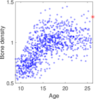
(a)

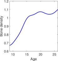
(b)

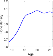
(c)

Figure 5: (a) Spinal bone mineral density data. (b) Estimated mean function. (c) Estimated mean function when the rightmost point in the left panel is removed from the data.

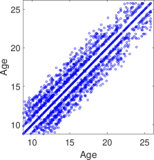
(a)

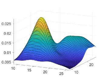
(b)

Figure 6: (a) Empirical design plot of the covariance structure of the spinal bone mineral density. (b) Estimated covariance function of the spinal bone mineral density, using the proposed method with Fourier basis and nonperiodic extension.

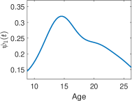
(a)

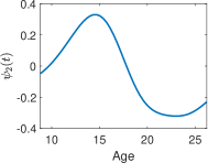
(b)

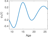
(c)

Figure 7: The first three principal components of spinal bone density data

5.2 Systolic Blood Pressure

We apply our method to the study of age-associated changes in blood pressure of healthy men using an anonymous data from the Baltimore Longitudinal Study of Aging (BLSA). In the study, 1590 healthy male volunteers (age 17–97) were scheduled to visit the Gerontology Research Center bi-annually. On each visit, systolic blood pressure (in mm Hg) was recorded along with other health related information. Measurements taken within 2 years of death (49 visits in 44 men) are excluded to avoid potential bias due to diseases that might interfere with blood pressure. The data have a sparse and irregular design as many visits were missed by participants or not on the schedule; see Pearson et al. (1997) for more details. Since there are very few data available beyond age 95, we restrict our focus to the age range 17–95. We also exclude subjects with only one visit. This results in a dataset of 1290 subjects, with approximate 7.5 visits per subject, shown in Figure 8(a).

From the design plot shown in Figure 9(a) for the covariance function, we see that there are no design points in the off-diagonal regions. Therefore, this is a dataset of functional snippets. Our estimated mean and covariance functions are shown in Figure 8(b) and Figure 9(b), respectively. We observe that the systolic blood pressure is relatively stable between 17 and 45, and then increases stiffly until the age 85. This is aligned with the discovery in Pearson et al. (1997). The slight downward trend after 85 could be due to insufficient data around the boundary. It could also be attributed, at least partly, to the selection effect (Müller et al., 1997; Wang et al., 1998): people with lifespan over 85, termed the oldest-old in aging research, are a selected group of subjects with favorable physical or genetic conditions.

The estimated covariance function suggests an increasing trend of variability of systolic blood pressure along the age. Similar to the mean function, the slight downward trend after 85 could be due to the selection effect or lack of data. We also utilize the estimated covariance function in the entire domain to provide the first three principal components, shown in Figure 10. These principal components account for 72.3%, 16.2% and 6.07% of the variance of the data, respectively. The first principal component function has a similar shape as the mean function, reflecting that the largest variation of systolic blood pressure is a vertical shift of the trajectory. This is a quite common phenomenon for functional data. The second principal component reflects the contrast before and after age 68. Those with positive second scores have higher than average systolic blood pressure before age 68 but lower than average systolic blood pressure after age 68. The third principal components depicts the contrast before and after age 50. Those with positive third scores have higher than average systolic blood pressure before age 50, with a peak around age 40, but lower than average blood pressure after age 50, probably due to change to a healthier life style.

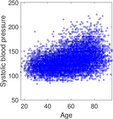
(a)

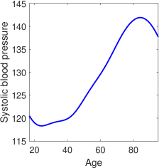
(b)

Figure 8: (a) Systolic blood pressure data. (b) Estimated mean function.

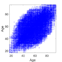
(a)

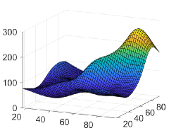
(b)

Figure 9: (a) Empirical design plot of the covariance structure of the systolic blood pressure. (b) Estimated covariance function of the systolic blood pressure, using the proposed method with Fourier basis and nonperiodic extension.

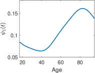
(a)

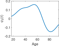
(b)

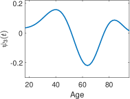
(c)

Figure 10: The first three principal components of systolic blood pressure data

Appendix A: Fourier Extension

For a nonperiodic function $g$, its finite Fourier series expansion $g_{N}$ is observed to suffer from the so-called Gibbs phenomenon (Zygmund, 2003) which refers to the drastic oscillatory overshoot in the region close to the two endpoints of the domain. A remedy to this issue is to employ the technique of Fourier extension mentioned in Example 5.

The idea of Fourier extension is to approximate a nonperiodic function $g$ by Fourier basis functions defined on an extended domain $\mathcal{T}_{\zeta}=[-\zeta,1+\zeta]$ for some $\zeta>0$ that we refer to as extension margin. The basis functions, are then defined by $\phi_{1}(t)=(1+2\zeta)^{-1/2}$, $\phi_{2k}(t)=\cos\{2k\pi t/(1+2\zeta)\}$ and $\phi_{2k-1}(t)=\sin\{2k\pi t/(1+2\zeta)\}$ for $k>1$. To elaborate, let $\mathscr{G}_{N}(\zeta)=\mathrm{span}\{\phi_{1},\ldots,\phi_{N}\}$. The Fourier extension of $g$ within $\mathscr{G}_{N}(\zeta)$, denoted by $\tilde{g}_{N}$, is defined by

$$\tilde{g}_{N}=\underset{h\in\mathscr{G}_{N}(\zeta)}{\arg\min}\,\|g-h\|_{L^{2}(0,1)},$$

where we emphasize that the norm $\|\cdot\|_{L^{2}(0,1)}$ is for the domain $\mathcal{T}$. One can easily see that the Fourier extension of $g$ is not unique. However, all such extensions have the same approximation quality for $g$ over the domain $\mathcal{T}$ of interest. Intuitively, for a Fourier extension of $g$, even if there is a Gibbs phenomenon, for a suitable $\zeta$, the phenomenon is expected to occur only within the extended part of the domain, i.e., $[-\zeta,0]$ and $[1,1+\zeta]$. Consequently, the nonperiodic function $g$ can then be well approximated on the domain $[0,1]$. Indeed, the speed of the convergence of a Fourier extension of $g$ in the domain $[0,1]$ adapts to the smoothness of $g$ (Adcock et al., 2014). For example, $\tilde{g}_{N}$ converges to $g$ at the rate of $N^{-r}$ ($c^{-N}$ for some $c>1$, respectively) when $g$ is $r$ times differentiable (analytic, respectively).

The above discussion can be straightforwardly extended to the two-dimensional case. Let $\mathscr{G}_{N}^{2}(\zeta)=\mathrm{span}\{\phi_{k}\otimes\phi_{l}:1\leq k,l\leq N\}$, where $\phi_{k}\otimes\phi_{l}$ represents the function $\phi_{k}(s)\phi_{l}(t)$ defined on the two-dimensional square $[-\zeta,1+\zeta]^{2}$. For a function $\gamma$ defined on $[0,1]^{2}$, its Fourier extension $\tilde{\gamma}$ within $\mathscr{G}_{N}^{2}(\zeta)$ is given by

$$\tilde{\gamma}_{N}=\underset{h\in\mathscr{G}_{N}^{2}(\zeta)}{\arg\min}\,\|\gamma-h\|_{L^{2}([0,1]^{2})},$$

where $L^{2}([0,1]^{2})$ denotes the space of squared integrable functions defined on $[0,1]^{2}$ with the norm $\|\gamma-h\|_{L^{2}([0,1]^{2})}=\{\int_{0}^{1}\int_{0}^{1}|\gamma(s,t)|^{2}\mathrm{d}s\mathrm{d}t\}^{1/2}$.

Appendix B: Geometric Newton Method

Let $\mathbf{C}=\mathbf{L}\mathbf{L}^{\top}$, where $\mathbf{L}$ is a lower triangular matrix whose diagonal elements are all positive. This is the so-called Cholesky decomposition of $\mathbf{C}$ and it is unique (since we require the diagonal elements of $\mathbf{L}$ to be positive). The objective function in (6) can be written as

$$Q(\mathbf{L})= \sum_{i=1}^{n}\mathrm{tr}[(\mathbf{R}_{i}-\mathbf{B}_{i}\mathbf{L}\mathbf{L}^{\top}\mathbf{B}_{i}^{\top})(\mathbf{R}_{i}-\mathbf{B}_{i}\mathbf{L}\mathbf{L}^{\top}\mathbf{B}_{i}^{\top})^{\top}]$$

$$-\sum_{i=1}^{n}\sum_{j=1}^{N_{i}}(\Gamma_{ijj}-\mathbf{b}_{ij}\mathbf{L}\mathbf{L}^{\top}\mathbf{b}_{ij}^{\top})^{2}$$

$$+\lambda\mathrm{tr}(\mathbf{\mathbf{L}\mathbf{L}^{\top}U\mathbf{L}\mathbf{L}^{\top}W}+\mathbf{\mathbf{L}\mathbf{L}^{\top}V\mathbf{L}\mathbf{L}^{\top}V}),$$

where $\mathbf{R}_{i}$ is a matrix whose $(j,k)$-entry is $\Gamma_{ijk}$, $\mathbf{B}_{i}$ is a matrix whose $(j,k)$-entry is $\phi_{j}(T_{ik})$ for $j=1,\ldots,p$ and $k=1,\ldots,m_{i}$, and $\mathbf{b}_{ij}$ is a row vector representing the $j$th row of $\mathbf{B}_{i}$. Instead of a constraint optimization problem in the space of all $p\times p$ lower triangular matrices, we view the minimization of $Q$ as an unconstrained optimization problem in the manifold of $p\times p$ lower triangular matrices whose diagonal elements are all positive, and then adopt Newton’s method on manifolds, as follows.

Informally speaking, a $d$-dimensional manifold $\mathcal{M}$ can be viewed as a subset of $\mathbb{R}^{D}$ for $d\leq D$, such that, for every $x\in\mathcal{M}$, there is a $d$-dimensional hyperplane $\mathbb{T}_{x}$ (of $\mathbb{R}^{D}$) that is tangential to $\mathcal{M}$ at $x$. If one endows the hyperplane $\mathbb{T}_{x}$ with an inner product, and the inner product (depending on $x$) varies smoothly with respect to $x$, then the manifold is called a Riemannian manifold. For a Riemannian manifold, for each $x$, there is an map $\mathrm{Exp}_{x}:\mathbb{T}_{x}\rightarrow\mathcal{M}$, called the Riemannian exponential map at $x$, such that for $u\in\mathbb{T}_{x}\subset\mathbb{R}^{D}$, $\mathrm{Exp}(u)=\psi(1)$ for a geodesic $\psi:[-1,1]\rightarrow\mathcal{M}$ passing through $x$ and $\psi^{\prime}(0)=u\in\mathbb{R}^{D}$. For an in-depth introduction to manifolds, we recommend the textbook by Lang (1995). For the manifold $\mathcal{M}=\{\mathbf{L}\in\mathbb{R}^{p\times p}:\,\mathbf{L}$ is lower triangular and has positive diagonal elements$\}$, Lin (2019) introduced a way to define smoothly varying inner products among the hyperplanes $\mathbb{T}_{\mathbf{X}}$ for $\mathbf{X}\in\mathcal{M}$, which turn $\mathcal{M}$ into a Riemannian manifold with Riemannian exponential map defined by $\mathrm{Exp}_{\mathbf{X}}\mathbf{S}=(\mathbf{X}-\mathbb{D}(\mathbf{X}))+(\mathbf{S}-\mathbb{D}(\mathbf{S}))+\mathbb{D}(\mathbf{X})\mathrm{expm}\{\mathbb{D}(\mathbf{S})\mathbb{D}(\mathbf{X})^{-1}\}$ for $\mathbf{X}\in\mathcal{M}$ and $\mathbf{S}\in\mathbb{T}_{\mathbf{X}}$, where $\mathbb{D}(\mathbf{X})$ denotes the diagonal matrix formed by the diagonal part of $\mathbf{X}$, and $\mathrm{expm}(\mathbf{A})=\sum_{k=0}^{\infty}\mathbf{A}^{k}/k!$, defined for any square matrix $\mathbf{A}$, denotes the matrix exponential function.

The geometric Newton method is the generalization of classic Newton method to Riemannian manifolds to compute a zero of a function $F(x)\in\mathbb{T}_{x}$. It can be used to solve our minimization problem by observing that if $Q(\mathbf{L})$ is (locally) minimized at $\mathbf{L}^{\ast}$ then $\partial Q/\partial\mathbf{L}$ vanishes at $\mathbf{L}^{\ast}$. In this case, $F(\mathbf{L})=\partial Q/\partial\mathbf{L}$. Starting with an initial point $\mathbf{L}_{0}\in\mathcal{M}$, for $k=0,1,\ldots$, we first solve the Newton equation

$$\mathcal{H}_{\mathbf{L}_{k}}\eta_{k}=-F(\mathbf{L}_{k})$$

for the unknown $\eta_{k}\in\mathbb{T}_{\mathbf{L}_{k}}$, where $\mathcal{H}_{\mathbf{L}}:\mathbb{T}_{\mathbf{L}}\rightarrow\mathbb{T}_{\mathbf{L}}$ denotes the gradient of $F$ (or equivalently, the Hessian of $Q$), and then set $\mathbf{L}_{k+1}=\mathrm{Exp}_{\mathbf{L}_{k}}(\eta_{k})$. The iteration is terminated if 1) $k\geq K$ for some specified integer $K>0$, 2) $\|F(\mathbf{L}_{k})\|_{2}\leq\epsilon$ for a tolerance level $\epsilon>0$, or 3) $\gamma_{{\mathbf{L}}_{k+1}{\mathbf{L}}_{k+1}^{\top}}\not\in\mathcal{C}$. One also needs to select an initial point $\mathbf{L}_{0}$, which is determined in the following way. We first minimize $Q$ with respect to $\mathbf{C}$ without considering the positive definiteness and the constraint $\gamma_{\mathbf{C}}\in\mathcal{C}$. In this case, $Q$ is a quadratic form of $\mathbf{C}$ and a closed-form solution is available. Denote the minimizer by $\check{\mathbf{C}}$. If $\check{\mathbf{C}}$ is not positive definite, we obtain its eigendecomposition $\check{\mathbf{C}}=\check{\mathbf{P}}\check{\Lambda}\check{\mathbf{P}}^{\top}$ for an orthogonal matrix $\check{\mathbf{P}}$ and a diagonal matrix $\check{\Lambda}$, and then set $\check{\mathbf{C}}=\check{\mathbf{P}}\mathring{\Lambda}\check{\mathbf{P}}^{\top}$, where $\mathring{\Lambda}$ is obtained from $\check{\Lambda}$ by setting its nonpositive diagonal elements to $0.01\times$largest singular value of $\check{\mathbf{C}}$.

It remains to compute the gradient $F$ and the Hessian $\mathcal{H}$ of the objective function $Q$. Straightforward computation shows that

$$F(\mathbf{L})= -4\sum_{i=1}^{n}\mathbf{B}_{i}^{\top}\mathbf{R}_{i}\mathbf{B}_{i}\mathbf{L}$$

$$+4\sum_{i=1}^{n}\mathbf{B}_{i}^{\top}\mathbf{B}_{i}\mathbf{L}\mathbf{L}^{\top}\mathbf{B}_{i}^{\top}\mathbf{B}_{i}\mathbf{L}$$

$$-4\sum_{i=1}^{n}\sum_{j=1}^{N_{i}}\mathbf{b}_{ij}^{\top}\mathbf{b}_{ij}\mathbf{L}\mathbf{L}^{\top}\mathbf{b}_{ij}^{\top}\mathbf{b}_{ij}\mathbf{L}$$

$$+4\sum_{i=1}^{n}\sum_{j=1}^{N_{i}}\Gamma_{ijj}\mathbf{b}_{ij}^{\top}\mathbf{b}_{ij}\mathbf{L}$$

$$+2\lambda\{\mathbf{U}\mathbf{L}\mathbf{L}^{\top}\mathbf{W}\mathbf{\mathbf{L}}+\mathbf{W}\mathbf{L}\mathbf{L}^{\top}\mathbf{U}\mathbf{L}\}$$

$$+4\lambda\mathbf{V}\mathbf{L}\mathbf{L}^{\top}\mathbf{V}\mathbf{\mathbf{L}}.$$

To compute the Hessian of $Q$, we first observe that, according to Proposition 5.5.4 of Absil et al. (2008),

$$\mathcal{H}_{\mathbf{L}}=\mathrm{Hess}(Q\circ\mathrm{Exp}_{\mathbf{L}})(0),$$

where $\circ$ denotes the composition of functions. Let $\mathbf{X}=\mathrm{Exp}_{\mathbf{L}}\mathbf{S}$ and $\Psi(\mathbf{S})=(Q\circ\mathrm{Exp}_{\mathbf{L}})(\mathbf{S})$. Then

$$\mathrm{grad}\Psi= -4\sum_{i=1}^{n}(\mathbf{B}_{i}^{\top}\mathbf{R}_{i}\mathbf{B}_{i}\mathbf{X})\odot\mathbf{Z}$$

$$+4\sum_{i=1}^{n}(\mathbf{B}_{i}^{\top}\mathbf{B}_{i}\mathbf{X}\mathbf{X}^{\top}\mathbf{B}_{i}^{\top}\mathbf{B}_{i}\mathbf{X})\odot\mathbf{Z}$$

$$-4\sum_{i=1}^{n}\sum_{j=1}^{N_{i}}(\mathbf{b}_{ij}^{\top}\mathbf{b}_{ij}\mathbf{X}\mathbf{X}^{\top}\mathbf{b}_{ij}^{\top}\mathbf{b}_{ij}\mathbf{X})\odot\mathbf{Z}$$

$$+4\sum_{i=1}^{n}\sum_{j=1}^{N_{i}}\Gamma_{ijj}(\mathbf{b}_{ij}^{\top}\mathbf{b}_{ij}\mathbf{X})\odot\mathbf{Z}$$

$$+2\lambda\{\mathbf{U}\mathbf{X}\mathbf{X}^{\top}\mathbf{W}\mathbf{\mathbf{X}}+\mathbf{W}\mathbf{X}\mathbf{X}^{\top}\mathbf{U}\mathbf{X}\}\odot\mathbf{Z}$$

$$+4\lambda(\mathbf{V}\mathbf{X}\mathbf{X}^{\top}\mathbf{V}\mathbf{\mathbf{X}})\odot\mathbf{Z},$$

where $\odot$ denotes matrix Hadamard product, and $\mathbf{Z}=\{z_{jk}\}$ is a $p\times p$ lower triangular matrix such that $z_{jk}=1$ if $k<j$ and $z_{jj}=e^{s_{jj}/L_{jj}}$ with $L_{jj}$ being the $(j,j)$-entry of $\mathbf{L}$. To compute the Hessian of $Q\circ\mathrm{Exp}_{\mathbf{L}}$ at $\mathbf{S}$, we proceed to compute the gradient of $\mathrm{grad}\Psi$. We first observe that, the terms in $\mathrm{grad}\Psi$ can be divided into two types: one is of the form $\mathbf{H}\mathbf{X}\odot\mathbf{Z}$, and the other is of the form $\mathbf{H}\mathbf{X}\mathbf{X}^{\top}\mathbf{G}\mathbf{\mathbf{X}}\odot\mathbf{Z}$, where $\mathbf{H}$ and $\mathbf{G}$ are some matrices not containing $\mathbf{X}$ or $\mathbf{S}$. Below we address them separately.

For the first type, let

$$\Xi_{jk}\equiv(\mathbf{H}\mathbf{\mathbf{X}})_{jk} =\sum_{\ell}h_{j\ell}x_{\ell k},$$

where $h_{j\ell}$ and $x_{\ell k}$ are the $(j,\ell)$- and $(\ell,k)$-entry of $\mathbf{H}$ and $\mathbf{X}$, respectively. Below we compute $\frac{\partial\Xi_{jk}}{\partial s_{\tau\nu}}$ for $1\leq k\leq j\leq p$ and $1\leq\nu\leq\tau\leq p$. When $k\neq\nu$, $L_{\ell k}$ does not contain $s_{\tau\nu}$, and thus

$$\frac{\partial\Xi_{jk}}{\partial s_{\tau\nu}}=\frac{\partial}{\partial s_{\tau\nu}}\sum_{\ell}h_{j\ell}x_{\ell k}=0.$$

When $k=\nu$, for $\nu=\tau$,

$$\frac{\partial\Xi_{jk}}{\partial s_{\tau\nu}}=\frac{\partial}{\partial s_{\tau\nu}}\sum_{\ell}h_{j\ell}x_{\ell k}=e^{s_{\tau\nu}/L_{\tau\nu}}h_{j\tau},$$

and for $\nu<\tau$,

$$\frac{\partial\Xi_{jk}}{\partial s_{\tau\nu}}=\frac{\partial}{\partial s_{\tau\nu}}\sum_{\ell}h_{j\ell}x_{\ell k}=h_{j\tau}.$$

To deal the second type, let

$$\Xi_{jk}\equiv(\mathbf{H}\mathbf{X}\mathbf{X}^{\top}\mathbf{G}\mathbf{\mathbf{X}})_{jk} =\sum_{\omega}\sum_{\ell}\sum_{a}\sum_{b}h_{j\omega}x_{\omega\ell}x_{a\ell}g_{ab}x_{bk}.$$

Now we compute $\frac{\partial\Xi_{jk}}{\partial s_{\tau\nu}}$ for $1\leq k\leq j\leq p$ and $1\leq\nu\leq\tau\leq p$. When $k\neq\nu$, for $\nu=\tau$,

$$\frac{\partial\Xi_{jk}}{\partial s_{\tau\nu}}=e^{s_{\tau\nu}/L_{\tau\nu}}\sum_{a}\sum_{b}(h_{j\tau}x_{a\nu}g_{ab}x_{bk})+e^{s_{\tau\nu}/L_{\tau\nu}}\sum_{\omega}\sum_{b}h_{j\omega}x_{\omega\nu}g_{\tau b}x_{bk},$$

and for $\nu<\tau$,

$$\frac{\partial\Xi_{jk}}{\partial s_{\tau\nu}} =\sum_{a}\sum_{b}h_{j\tau}x_{a\nu}g_{ab}x_{bk}+\sum_{\omega}\sum_{b}h_{j\omega}x_{\omega\nu}g_{\tau b}x_{bk}$$

$$=h_{j\tau}\mathbf{X}_{\cdot\nu}^{\top}\mathbf{G}\mathbf{X}_{\cdot k}+\mathbf{H}_{j\cdot}\mathbf{X}_{\cdot\nu}\mathbf{G}_{\tau\cdot}\mathbf{X}_{\cdot k},$$

where the notation $\mathbf{X}_{\cdot k}$ denotes the $k$th column of the matrix $\mathbf{X}$, and $\mathbf{G}_{\tau\cdot}$ denotes the $\tau$th row of $\mathbf{G}$.

When $k=\nu$, for $\tau=\nu$,

$$\frac{\partial\Xi_{jk}}{\partial s_{\tau\nu}} =e^{s_{\tau\nu}/L_{\tau\nu}}\left(\sum_{a}\sum_{b}h_{j\tau}x_{a\nu}g_{ab}x_{bk}+\sum_{\ell}\sum_{b}h_{j\ell}x_{\ell\nu}g_{\tau b}x_{bk}+\sum_{\omega}\sum_{\ell}\sum_{a}h_{j\omega}x_{\omega\ell}x_{a\ell}g_{a\tau}\right)$$

$$=e^{s_{\tau\nu}/L_{\tau\nu}}(h_{j\tau}\mathbf{X}_{\cdot\nu}^{\top}\mathbf{G}\mathbf{X}_{\cdot k}+\mathbf{H}_{j\cdot}\mathbf{X}_{\cdot\nu}\mathbf{G}_{\tau\cdot}\mathbf{X}_{\cdot k}+\mathbf{H}_{j\cdot}\mathbf{X}\mathbf{X}^{\top}\mathbf{G}_{\cdot\tau}),$$

and for $\nu<\tau$,

$$\frac{\partial\Xi_{jk}}{\partial s_{\tau\nu}} =\sum_{a}\sum_{b}h_{j\tau}x_{a\nu}g_{ab}x_{bk}+\sum_{\omega}\sum_{b}h_{j\omega}x_{\omega\nu}g_{\tau b}x_{bk}+\sum_{\omega}\sum_{\ell}\sum_{a}h_{j\omega}x_{\omega\ell}x_{a\ell}g_{a\tau}$$

$$=h_{j\tau}\mathbf{X}_{\cdot\nu}^{\top}\mathbf{G}\mathbf{X}_{\cdot k}+\mathbf{H}_{j\cdot}\mathbf{X}_{\cdot\nu}\mathbf{G}_{\tau\cdot}\mathbf{X}_{\cdot k}+\mathbf{H}_{j\cdot}\mathbf{X}\mathbf{X}^{\top}\mathbf{G}_{\cdot\tau}.$$

Appendix C: Technical Proofs

Notation.

Without loss of generality, we assume $\mathcal{T}=[0,1]$. We use $\boldsymbol{\Phi}_{q}$ to denote the column vector $(\phi_{1},\ldots,\phi_{q})^{\top}$, and $\boldsymbol{\Phi}_{q}(t)$ to denote its value evaluated at $t$. The $\ell^{2}$ norm of a vector $\mathbf{v}$ is denoted by $\|\mathbf{v}\|_{2}$. When $\mathbf{v}$ is viewed as a linear functional, its operator norm is denoted by $\|\mathbf{v}\|$. Note that $\|\mathbf{v}\|=\|\mathbf{v}\|_{2}$. For a matrix $\mathbf{M}$, $\|\mathbf{M}\|$ denotes its induced operator norm, while $\|\mathbf{M}\|_{\mathrm{F}}$ denotes its Frobenius norm. For a function $\mu$ defined on $\mathcal{T}$, its $L^{2}$ norm, denoted by $\|\mu\|_{L^{2}}$, is defined by $\|\mu\|_{L^{2}}=\{\int_{\mathcal{T}}|\mu(t)|^{2}\mathrm{d}t\}^{1/2}$. For a covariance function $\gamma$, we use $\|\gamma\|_{L^{2}}$ to denote its $L^{2}$ norm that is defined by $\|\gamma\|_{L^{2}}=\{\int_{\mathcal{T}^{2}}|\gamma(s,t)|^{2}\mathrm{d}s\mathrm{d}t\}^{1/2}$.

Proof of Theorem 1.

In the sequel, we use $\mathbf{a}$ to denote the vector of the coefficients of $\mu_{0}$ with respect to the basis functions $\phi_{1},\ldots,\phi_{p}$.

First, we observe that, $\mathfrak{c}_{1}\mathfrak{c}_{3}\delta/2\leq f_{T}(t)\leq\mathfrak{c}_{2}\mathfrak{c}_{4}\delta$ for all $t\in[0,1]$. Let $C_{1}=\min\{\mathfrak{c}_{1},\mathfrak{c}_{3},\mathfrak{c}_{1}\mathfrak{c}_{3}\delta/2\}$, $C_{2}=\max\{\mathfrak{c}_{2},\mathfrak{c}_{4},\mathfrak{c}_{2}\mathfrak{c}_{4}\delta\}$ and $\varrho_{n}\asymp n^{-1/2}q^{\alpha+1/2}+\tau_{q}$. Define

$$Q(\mathbf{a})=\frac{1}{nm}\sum_{i=1}^{n}\sum_{j=1}^{m}\{Y_{ij}-\mathbf{a}^{\top}\boldsymbol{\Phi}_{q}(T_{ij})\}^{2}+\rho H(\mathbf{a}^{\top}\boldsymbol{\Phi}_{q}).$$

Then we observe that

$$Q(\mathbf{a}+\varrho_{n}\mathbf{u})-Q(\mathbf{a})$$

$$= -\frac{2\varrho_{n}}{nm}\sum_{i=1}^{n}\sum_{j=1}^{m}\mathbf{u}^{\top}\boldsymbol{\Phi}_{q}(T_{ij})\{Y_{ij}-\mathbf{a}^{\top}\boldsymbol{\Phi}_{q}(T_{ij})\}+\frac{\varrho_{n}^{2}}{nm}\sum_{i=1}^{n}\sum_{j=1}^{m}\{\mathbf{u}^{\top}\boldsymbol{\Phi}_{q}(T_{ij})\}^{2}$$

$$+2\rho\varrho_{n}\mathbf{u}^{\top}\mathbf{W}\mathbf{a}+\rho\varrho_{n}^{2}\mathbf{u}^{\top}\mathbf{W}\mathbf{u}$$

$$\equiv -2\varrho_{n}\mathrm{I}+\varrho_{n}^{2}\mathrm{II}+2\rho\varrho_{n}\mathrm{III}+\rho\varrho_{n}^{2}\mathrm{IV}.$$ (11)

It is easy to check that $\|\mathbf{W}\|\leq\|\mathbf{W}\|_{\mathrm{F}}=O(q^{4\beta+1})$. Thus, $|\mathrm{III}|=O(q^{4\beta+1})\|\mathbf{u}\|_{2}$ and $|\mathrm{IV}|=O(q^{4\beta+1})\|\mathbf{u}\|_{2}^{2}$. According to Claim 1 and 2, we have that, for any $\epsilon>0$, there exists $N_{\epsilon}>0$, $\theta_{\epsilon}>0$, and $\Omega_{n,\epsilon}\subset\Omega$, such that for all $n\geq N_{\epsilon}$,

• $\mathbb{P}(\Omega_{n,\epsilon})\geq 1-\epsilon$, and

• for all $\omega\in\Omega_{n,\epsilon}$, $|\mathrm{I}|=|\mathrm{I}(\omega)|\leq\theta_{\epsilon}(n^{-1/2}q^{\alpha+1/2+\tau_{q}})\|\mathbf{u}\|_{2}$, and

• for all $\omega\in\Omega_{n,\epsilon}$, $|\mathrm{II}|=|\mathrm{II}(\omega)|\geq C_{1}\|\mathbf{u}\|_{2}^{2}/2$,

where $\Omega$ denotes the sample space. With the choice of $\varrho_{n}$ and $\rho$, we can see that $Q(\mathbf{a}+\varrho_{n}\mathbf{u})-Q(\mathbf{a})>0$ on $\Omega_{n,\epsilon}$ for all $\mathbf{u}$ with $\|\mathbf{u}\|_{2}=D_{\epsilon}$ for a sufficiently large and fixed constant $D_{\epsilon}>0$. Therefore, with probability tending to one, the minimizer $\hat{\mathbf{a}}$ of $Q$ falls into the ball $\{\mathbf{u}\in\mathbb{R}^{q}:\|\mathbf{u}-\mathbf{a}\|_{2}\leq D_{\epsilon}\varrho_{n}\}$. Now,

$$\|\hat{\mu}-\mu_{0}\|_{L^{2}}^{2}\leq 2\|\hat{\mu}-\mathbf{a}^{\top}\boldsymbol{\Phi}_{q}\|_{L^{2}}^{2}+2\|\mathbf{a}^{\top}\boldsymbol{\Phi}_{q}-\mu_{0}\|_{L^{2}}^{2}=O_{P}(\varrho_{n}^{2}+\tau_{q}^{2}),$$

and the proof of the theorem is completed. ∎

Claim 1.

For any $\epsilon>0$, there exists $N_{\epsilon}>0$, $\theta_{\epsilon}>0$, and $\Omega_{n,\epsilon}\subset\Omega$, such that for all $n\geq N_{\epsilon}$,

• $\mathbb{P}(\Omega_{n,\epsilon})\geq 1-\epsilon$, and

• for all $\omega\in\Omega_{n,\epsilon}$, $|\mathrm{I}|=|\mathrm{I}(\omega)|\leq\theta_{\epsilon}(n^{-1/2}q^{\alpha+1/2}+\tau_{q})\|\mathbf{u}\|_{2}$, where $\mathrm{I}$ is given in (11).

Proof.

We first observe that

$$\mathrm{I} =\frac{1}{nm}\sum_{i=1}^{n}\sum_{j=1}^{m}\mathbf{u}^{\top}\boldsymbol{\Phi}_{q}(T_{ij})\{Y_{ij}-\mu_{0}(T_{ij})+\mu_{0}(T_{ij})-\mathbf{a}^{\top}\boldsymbol{\Phi}_{q}(T_{ij})\}$$

$$=\frac{1}{nm}\sum_{i=1}^{n}\sum_{j=1}^{m}\mathbf{u}^{\top}\boldsymbol{\Phi}_{q}(T_{ij})\{Y_{ij}-\mu_{0}(T_{ij})\}+\frac{1}{nm}\sum_{i=1}^{n}\sum_{j=1}^{m}\mathbf{u}^{\top}\boldsymbol{\Phi}_{q}(T_{ij})\{\mu_{0}(T_{ij})-\mathbf{a}^{\top}\boldsymbol{\Phi}_{q}(T_{ij})\}$$

$$\equiv\mathrm{I}_{1}+\mathrm{I}_{2}.$$

Now we consider the first term $\mathrm{I}_{1}$. Let $\mathbf{s}=\frac{1}{nm}\sum_{i=1}^{n}\sum_{j=1}^{m}\{Y_{ij}-\mu_{0}(T_{ij})\}\boldsymbol{\Phi}_{q}(T_{ij})$. We treat it as a linear functional on the Euclidean space $(\mathbb{R}^{q},\|\cdot\|_{2})$. It is seen that $\mathbb{E}\mathbf{s}=0$. Note that the operator norm of $\mathbf{s}$ is equal to its $\ell^{2}$ norm. Then,

$$\mathbb{V}(\|\mathbf{s}\|) \leq\mathbb{E}\|\mathbf{s}\|^{2}=\mathbb{E}\|\mathbf{s}\|_{2}^{2}$$

$$=\sum_{1\leq l\leq q}\mathbb{E}\left(\frac{1}{nm}\sum_{i=1}^{n}\sum_{j=1}^{m}\{Y_{ij}-\mu_{0}(T_{ij})\}\phi_{l}(T_{ij})\right)^{2}$$

$$=\frac{1}{n}\sum_{1\leq l\leq q}\mathbb{E}\left(\frac{1}{m}\sum_{j=1}^{m}\{Y_{1j}-\mu_{0}(T_{1j})\}\phi_{l}(T_{1j})\right)^{2}$$

$$=O(n^{-1}q^{2\alpha+1}),$$

where the last equation is obtained with the aid of the assumption that $\|\phi_{k}\|_{\infty}=O(k^{\alpha})$ uniformly over all $k$, as the basis is assumed to be an $(\alpha,\beta)$-basis. The above derivation also shows that $\mathbb{E}\|\mathbf{s}\|_{2}\leq(\mathbb{E}\|\mathbf{s}\|_{2}^{2})^{1/2}=O(n^{-1/2}q^{\alpha+1/2})$, Thus,

$$\sup_{\mathbf{u}\neq 0}\frac{|\mathrm{I}_{1}|}{\|\mathbf{u}\|_{2}}=\sup_{\mathbf{u}\neq 0}\frac{\|\mathbf{s}^{\top}\mathbf{u}\|_{2}}{\|\mathbf{u}\|_{2}}\leq\|\mathbf{s}\|_{2}=O_{P}(n^{-1/2}q^{\alpha+1/2}).$$ (12)

Similar argument shows that

$$\mathrm{I}_{2}-\mathbb{E}\mathrm{I}_{2}=O_{P}(n^{-1/2}q^{\alpha+1/2}).$$ (13)

In addition,

$$|\mathbb{E}\mathrm{I}_{2}| =|\mathbb{E}\mathbf{u}^{\top}\boldsymbol{\Phi}_{q}(T_{11})\{\mu_{0}(T_{11})-\mathbf{a}^{\top}\boldsymbol{\Phi}_{q}(T_{11})\}|$$

$$\leq[\mathbb{E}\{\mathbf{u}^{\top}\boldsymbol{\Phi}_{q}(T_{11})\}^{2}]^{1/2}[\mathbb{E}\{\mu_{0}(T_{11})-\mathbf{a}^{\top}\boldsymbol{\Phi}_{q}(T_{11})\}^{2}]^{1/2}$$

$$=O(1)\|\mathbf{u}\|_{2}\cdot O(1)\|\mu_{0}-\mathbf{a}^{\top}\boldsymbol{\Phi}_{q}\|_{L^{2}}$$

$$=O(\tau_{q})\|\mathbf{u}\|_{2}.$$

Combined with (12) and (13), this proves the claim. ∎

Claim 2.

Suppose $q^{2\alpha+2}n^{-1}\rightarrow 0$. Then, for any $\epsilon>0$, there exists $N_{\epsilon}>0$, and $\Omega_{n,\epsilon}\subset\Omega$, such that for all $n\geq N_{\epsilon}$,

• $\mathbb{P}(\Omega_{n,\epsilon})\geq 1-\epsilon$, and

• for all $\omega\in\Omega_{n,\epsilon}$, $|\mathrm{II}|=|\mathrm{II}(\omega)|\geq C_{1}\|\mathbf{u}\|_{2}^{2}/2$, where $\mathrm{II}$ is given in (11).

Proof.

Let $\mathbf{B}=n^{-1}m^{-1}\sum_{i}\sum_{j}\boldsymbol{\Phi}_{q}^{\top}(T_{ij})\boldsymbol{\Phi}_{q}(T_{ij})$ and $\mathbf{E}=\mathbb{E}\mathbf{B}$. Now we derive the bound for the smallest eigenvalue $\underline{\Lambda}(\mathbf{E})$ of $\mathbf{E}$. As $\mathbf{E}$ is positive semi-positive definite, one has

$$\underline{\Lambda}(\mathbf{E})=\inf_{\|\mathbf{u}\|_{2}=1}\mathbf{u}^{\top}\mathbf{E}\mathbf{u}.$$

Let $E_{jk}$ be the element of $\mathbf{E}$ at the $j$th row and $k$th column. Note that

$$E_{jk}=\mathbb{E}\{\phi_{j}(T)\phi_{k}(T)\}=\int_{0}^{1}\phi_{j}(t)\phi_{k}(t)f_{T}(t)\mathrm{d}t.$$

Thus,

$$\mathbf{u}^{\top}\mathbf{E}\mathbf{u} =\sum_{j,k}u_{j}E_{jk}u_{k}=\int_{0}^{1}f_{T}(t)\left(\sum_{j}u_{j}\phi_{j}(t)\right)^{2}\mathrm{d}t$$

$$\geq C_{1}\int_{0}^{1}\left(\sum_{j}u_{j}\phi_{j}(t)\right)^{2}\mathrm{d}t=C_{1}\|\mathbf{u}\|_{2}^{2},$$

where the last inequality is due to the orthonormality of $\{\phi_{k}\}$. Thus,

$$\underline{\Lambda}(\mathbf{E})\geq C_{1}.$$

Observe that $\mathbf{B}=\mathbf{E}+\Delta$ with $\Delta=\mathbf{B}-\mathbf{E}$. We then have $\mathbb{E}\Delta=\mathbf{0}$ and

$$\mathbb{V}(\|\Delta\|) \leq\mathbb{E}\|\Delta\|^{2}\leq\mathbb{E}\|\Delta\|_{\mathrm{F}}^{2}$$

$$\leq\sum_{1\leq l,h\leq q}\mathbb{E}\left(n^{-1}m^{-1}\sum_{i}\sum_{j}\phi_{l}(T_{ij})\phi_{h}(T_{ij})-E_{lh}\right)^{2}$$

$$=\sum_{1\leq l,h\leq q}\frac{1}{n}\mathbb{E}\left(\frac{1}{m}\sum_{j}\phi_{l}(T_{1j})\phi_{h}(T_{1j})-E_{lh}\right)^{2}$$

$$=O(q^{2\alpha+2}n^{-1}).$$

Now the claim follows from Weyl’s inequality. ∎

Proof of Theorem 2 and 3.

Theorem 2 is a special case of Theorem 3 with $\eta=0$. Below we prove Theorem 3. In the sequel, we use $\tilde{\mathbf{C}}$ to denote the matrix formed by the coefficients of $\tilde{\gamma}$ with respect to the basis functions $\{\phi_{k}\otimes\phi_{l}:\,1\leq k,l\leq p\}$.

Let $\varrho_{n}=p^{2\alpha+1}n^{-1/2}+\kappa_{p}+\eta$ and

$$\mathcal{B}_{p}(\theta)=\{\mathbf{D}:\|\mathbf{D}\|_{\mathrm{F}}=\theta,\tilde{\mathbf{C}}+\mathbf{D}\in\mathfrak{C}(p)\},$$ (14)

where ${\mathfrak{C}}(p)$ denotes the collection of $p\times p$ symmetric matrices $\mathbf{G}=[g_{kl}]$ such that $\gamma_{\mathbf{G}}=\sum_{1\leq k,l\leq p}g_{kl}\phi_{k}\otimes\phi_{l}\in\mathcal{C}$. For any $p\times p$ matrix $\mathbf{C}$, define

$$Q(\mathbf{C})=\frac{1}{nm(m-1)}\sum_{i=1}^{n}\sum_{1\leq j\neq k\leq m}\{\Gamma_{ijk}-\gamma_{\mathbf{C}}(T_{ij},T_{ik})\}^{2}+\lambda J(\gamma_{\mathbf{C}}).$$

Then we observe that

$$Q(\tilde{\mathbf{C}}+\varrho_{n}\mathbf{D})-Q(\tilde{\mathbf{C}})$$

$$= -2\varrho_{n}\frac{1}{nm(m-1)}\sum_{i=1}^{n}\sum_{1\leq j\neq k\leq m}\{\Gamma_{ijk}-\gamma_{\tilde{\mathbf{C}}}(T_{ij},T_{ik})\}\boldsymbol{\Phi}_{p}^{\top}(T_{ij})\mathbf{D}\boldsymbol{\Phi}_{p}(T_{ik})$$

$$+\varrho_{n}^{2}\frac{1}{nm(m-1)}\sum_{i=1}^{n}\sum_{1\leq j\neq k\leq m}\{\boldsymbol{\Phi}_{p}^{\top}(T_{ij})\mathbf{D}\boldsymbol{\Phi}_{p}(T_{ik})\}^{2}$$

$$+2\lambda\varrho_{n}\{\mathrm{tr}(\mathbf{DW}\tilde{\mathbf{C}}\mathbf{U})+\mathrm{tr}(\mathbf{D}\mathbf{V}\tilde{\mathbf{C}}\mathbf{V})\}$$

$$+\lambda\varrho_{n}^{2}\{\mathrm{tr}(\mathbf{DU}\mathbf{D}\mathbf{W})+\mathrm{tr}(\mathbf{D}\mathbf{V}\mathbf{D}\mathbf{V})\}$$

$$\equiv -2\varrho_{n}\mathrm{I}+\varrho_{n}^{2}\mathrm{II}+2\lambda\varrho_{n}\mathrm{III}+\lambda\varrho_{n}^{2}\mathrm{IV}.$$ (15)

Note that $\mathrm{tr}(\mathbf{A})\leq\sqrt{p}\|\mathbf{A}\|_{\mathrm{F}}$ for any $p\times p$ matrix $\mathbf{A}$. With the the assumption that $\|\phi_{k}^{(r)}\|_{L^{2}}=O(k^{\beta r})$ for $r=1,2$, one can then check that $|\mathrm{tr}(\mathbf{DW}\tilde{\mathbf{C}}\mathbf{U})|=O(p^{4\beta+5/2})\|\mathbf{D}\|_{\mathrm{F}}$, $|\mathrm{tr}(\mathbf{D}\mathbf{V}\tilde{\mathbf{C}}\mathbf{V})|=O(p^{4\beta+5/2})\|\mathbf{D}\|_{\mathrm{F}}$, $|\mathrm{tr}(\mathbf{DU}\mathbf{D}\mathbf{W})|=O(p^{4\beta+5/2})\|\mathbf{D}\|_{\mathrm{F}}^{2}$ and $|\mathrm{tr}(\mathbf{D}\mathbf{V}\mathbf{D}\mathbf{V})|=O(p^{4\beta+5/2})\|\mathbf{D}\|_{\mathrm{F}}^{2}$ by using the fact that $\|\mathbf{U}\|_{\mathrm{F}}^{2}=O(p^{2})$, $\|\mathbf{W}\|_{\mathrm{F}}^{2}=O(p^{8\beta+2})$, $\|\mathbf{V}\|_{\mathrm{F}}^{2}=O(p^{4\beta+2})$ and $\|\tilde{\mathbf{C}}\|_{\mathrm{F}}\leq\|\gamma_{0}\|_{L^{2}}+\eta=O(1)$. These give the orders of the terms $\mathrm{III}$ and $\mathrm{IV}$, which are $O(p^{4\beta+5/2})\|\mathbf{D}\|_{\mathrm{F}}$ and $O(p^{4\beta+5/2})\|\mathbf{D}\|_{\mathrm{F}}^{2}$, respectively.

According to Claim 3 and 4, now we have that, for any $\epsilon>0$, there exists $N_{\epsilon}>0$, $\theta_{\epsilon}>0$, and $\Omega_{n,\epsilon}\subset\Omega$, such that for all $n\geq N_{\epsilon}$,

• $\mathbb{P}(\Omega_{n,\epsilon})\geq 1-\epsilon$, and

• for all $\omega\in\Omega_{n,\epsilon}$, $|\mathrm{I}|=|\mathrm{I}(\omega)|\leq\theta_{\epsilon}(p^{2\alpha+1}n^{-1/2}+\kappa_{p}+\eta)\|\mathbf{D}\|_{\mathrm{F}}$, and

• for all $\omega\in\Omega_{n,\epsilon}$, $|\mathrm{II}|=|\mathrm{II}(\omega)|\geq\theta_{1}\|\mathbf{D}\|_{\mathrm{F}}^{2}$, where the constant $\theta_{1}>0$ depends only on $f_{R}$, $f_{T\mid R}$, $\gamma_{0}$ and $\mathcal{C}$.

With the choice of $\varrho_{n}$ and $\lambda$, we can see that $Q(\tilde{\mathbf{C}}+\varrho_{n}\mathbf{D})-Q(\tilde{\mathbf{C}})>0$ on $\Omega_{n,\epsilon}$ for all $\mathbf{D}\in\mathcal{B}_{p}(\theta)$ for all sufficiently large and fixed constant $\theta>0$. Therefore, with probability tending to one, the minimizer $\hat{\mathbf{C}}$ of $Q$ falls into $\{\mathbf{G}\in\mathfrak{C}(p):\|\mathbf{G}-\tilde{\mathbf{C}}\|_{\mathrm{F}}\leq\varrho_{n}\theta\}$. Therefore,

$$\|\hat{\gamma}-\gamma_{0}\|_{L^{2}}\leq\|\hat{\gamma}-\boldsymbol{\Phi}_{p}^{\top}\tilde{\mathbf{C}}\boldsymbol{\Phi}_{p}\|_{L^{2}}+\|\boldsymbol{\Phi}_{p}^{\top}\tilde{\mathbf{C}}\boldsymbol{\Phi}_{p}-\tilde{\gamma}\|_{L^{2}}+\|\tilde{\gamma}-\gamma_{0}\|_{L^{2}}=O_{P}(\varrho_{n}+\kappa_{p}+\eta),$$

and the proof of the theorem is completed. ∎

Claim 3.

For any $\epsilon>0$, there exists $N_{\epsilon}>0$, $\theta_{\epsilon}>0$, and $\Omega_{n,\epsilon}\subset\Omega$, such that for all $n\geq N_{\epsilon}$,

• $\mathbb{P}(\Omega_{n,\epsilon})\geq 1-\epsilon$, and

• for all $\omega\in\Omega_{n,\epsilon}$, $|\mathrm{I}|=|\mathrm{I}(\omega)|\leq\theta_{\epsilon}(p^{2\alpha+1}n^{-1/2}+\kappa_{p}+\eta)\|\mathbf{D}\|_{\mathrm{F}}$, where $\mathrm{I}$ is given in (15).

Proof.

We first observe that

$$\mathrm{I}= \frac{1}{nm(m-1)}\sum_{i=1}^{n}\sum_{1\leq j\neq k\leq m}\{\Gamma_{ijk}-\gamma_{0}(T_{ij},T_{ik})\}\boldsymbol{\Phi}_{p}^{\top}(T_{ij})\mathbf{D}\boldsymbol{\Phi}_{p}(T_{ik})$$

$$+\frac{1}{nm(m-1)}\sum_{i=1}^{n}\sum_{1\leq j\neq k\leq m}\{\gamma_{0}(T_{ij},T_{ik})-\gamma_{\tilde{\mathbf{C}}}(T_{ij},T_{ik})\}\boldsymbol{\Phi}_{p}^{\top}(T_{ij})\mathbf{D}\boldsymbol{\Phi}_{p}(T_{ik})$$

$$\equiv \mathrm{I}_{1}+\mathrm{I}_{2}.$$

Now we consider the first term $\mathrm{I}_{1}$. Let $\mathbf{S}=\frac{1}{nm(m-1)}\sum_{i=1}^{n}\sum_{1\leq j\neq k\leq m}[\{Y_{ij}-\mu_{0}(T_{ij})\}\{Y_{ik}-\mu_{0}(T_{ik})\}-\gamma_{0}(T_{ij},T_{ik})]\boldsymbol{\Phi}_{p}^{\top}(T_{ij})\odot\boldsymbol{\Phi}_{p}^{\top}(T_{ik})$, where $\odot$ denotes the Kronecker product of matrices. This $\mathbf{S}$ is viewed as a random linear functional acting on $\overrightarrow{\mathbf{D}}\in\mathbb{R}^{p^{2}}$, where $\overrightarrow{\mathbf{D}}$ denotes the vectorization of $\mathbf{D}$ obtained by stacking the columns of $\mathbf{D}$ into a single column vector. To quantify the order of its operator norm $\|\mathbf{S}\|$, we first observe that $\mathbb{E}\mathbf{S}=0$. Noting the operator norm is bounded by the Frobenius norm, we deduce that

$$\mathbb{V}(\|\mathbf{S}\|)\leq\mathbb{E}\|\mathbf{S}\|_{\mathrm{F}}^{2}$$

$$=\frac{1}{n}\sum_{1\leq l,h\leq p}\mathbb{E}\left(\frac{1}{m(m-1)}\sum_{1\leq j\neq k\leq m}[\{Y_{ij}-\mu_{0}(T_{ij})\}\{Y_{ik}-\mu_{0}(T_{ik})\}-\gamma_{0}(T_{ij},T_{ik})]\phi_{l}(T_{ij})\phi_{h}(T_{ik})\right)^{2}$$

$$\leq\frac{1}{n}\frac{1}{m(m-1)}\sum_{1\leq l,h\leq p}\sum_{1\leq j\neq k\leq m}\mathbb{E}\left([\{Y_{1j}-\mu_{0}(T_{1j})\}\{Y_{1k}-\mu_{0}(T_{1k})\}-\gamma_{0}(T_{1j},T_{1k})]\phi_{l}(T_{1j})\phi_{h}(T_{1k})\right)^{2}$$

$$=O(n^{-1})\sum_{1\leq l,h\leq p}l^{2\alpha}h^{2\alpha}\sum_{1\leq j\neq k\leq m}\mathbb{E}\left([\{Y_{1j}-\mu_{0}(T_{1j})\}\{Y_{1k}-\mu_{0}(T_{1k})\}-\gamma_{0}(T_{1j},T_{1k})]\right)^{2}$$

$$=O\left(\frac{p^{4\alpha+2}}{n}\right)\mathbb{E}[\{Y_{11}-\mu_{0}(T_{11})\}\{Y_{12}-\mu_{0}(T_{12})\}-\gamma_{0}(T_{11},T_{12})]^{2}$$

$$=O\left(\frac{p^{4\alpha+2}}{n}\right)(\mathbb{E}[\{Y_{11}-\mu_{0}(T_{11})\}\{Y_{12}-\mu_{0}(T_{12})\}]^{2}+\mathbb{E}[\gamma_{0}(T_{11},T_{12})]^{2})$$

$$=O(p^{4\alpha+2}n^{-1}),$$

where the last equation is due to the fact that $\gamma_{0}$ is continuous and thus bounded on $[0,1]^{2}$, and the fact that, with the notation $Z_{1}=X_{1}-\mu_{0}$,

$$\mathbb{E}[\{Y_{11}-\mu_{0}(T_{11})\}\{Y_{12}-\mu_{0}(T_{12})\}]^{2}$$

$$=\mathbb{E}[\{Z_{1}(T_{11})+\varepsilon_{11})\}\{Z_{1}(T_{12})+\varepsilon_{12}\}]^{2}$$

$$\leq 4\mathbb{E}\{Z_{1}^{2}(T_{11})+\varepsilon_{11}^{2}\}\{Z_{1}^{2}(T_{12})+\varepsilon_{12}^{2}\}$$

$$=4\mathbb{E}\{Z_{1}^{2}(T_{11})Z_{1}^{2}(T_{12})\}+O(\mathbb{E}\|Z_{1}\|^{2}_{L^{2}})+O(1)$$

$$=4\mathbb{E}[\mathbb{E}\{Z_{1}^{2}(T_{11})\mid O_{1},Z_{1}\}\mathbb{E}\{Z_{1}^{2}(T_{12})\mid O_{1},Z_{1}\}]+O(\mathbb{E}\|X\|^{2}_{L^{2}})+O(1)$$

$$=O(\mathbb{E}\{\|Z_{1}\|^{2}_{L^{2}}\|Z_{1}\|^{2}_{L^{2}}\})+O(\mathbb{E}\|X\|^{2}_{L^{2}})+O(1)$$

$$=O(\mathbb{E}\{\|X\|^{4}_{L^{2}})+O(\mathbb{E}\|X\|^{2}_{L^{2}})+O(1)$$

$$=O(1),$$

since $\mathbb{E}\|X\|^{4}_{L^{2}}<\infty$ which also implies $\mathbb{E}\|X\|^{2}_{L^{2}}<\infty$. Thus,

$$\sup_{\mathbf{D}\neq 0}\frac{|\mathrm{I}_{1}|}{\|\mathbf{D}\|_{\mathrm{F}}}=\sup_{\mathbf{D}\neq 0}\frac{|\mathbf{S}\overrightarrow{\mathbf{D}}|}{\|\mathbf{D}\|_{\mathrm{F}}} \leq\|\mathbf{S}\|_{\mathrm{F}}=O(p^{2\alpha+1}n^{-1/2}).$$

Therefore,

$$\mathrm{I}_{1}=O_{P}(p^{2\alpha+1}n^{-1/2})\|\mathbf{D}\|_{\mathrm{F}},$$ (16)

where the term $O_{P}(\cdot)$ is uniform over all $\mathbf{D}$.

Similar derivation combined with the strategy for establishing (13) shows that

$$\mathrm{I}_{2}-\mathbb{E}\mathrm{I}_{2}=O_{P}(p^{2\alpha+1}n^{-1/2})\|\mathbf{D}\|_{\mathrm{F}}.$$ (17)

In addition,

$$|\mathbb{E}\mathrm{I}_{2}| =|\mathbb{E}[\{\gamma_{0}(T_{11},T_{12})-\gamma_{\tilde{\mathbf{C}}}(T_{11},T_{12})\}\boldsymbol{\Phi}_{p}^{\top}(T_{11})\mathbf{D}\boldsymbol{\Phi}_{p}(T_{12})]|$$

$$\leq[\mathbb{E}\{\gamma_{0}(T_{11},T_{12})-\gamma_{\tilde{\mathbf{C}}}(T_{11},T_{12})\}^{2}]^{1/2}[\mathbb{E}\{\boldsymbol{\Phi}_{p}^{\top}(T_{11})\mathbf{D}\boldsymbol{\Phi}_{p}(T_{12})\}^{2}]^{1/2}$$

$$\leq O(1)\|\gamma_{0}-\gamma_{\tilde{\mathbf{C}}}\|_{\mathrm{F}}\cdot O(1)\|\mathbf{D}\|_{\mathrm{F}}$$

$$\leq O(\kappa_{p}+\eta)\|\mathbf{D}\|_{\mathrm{F}}.$$

The claim then follows from the above derivation, (16), and (17). ∎

Claim 4.

Suppose $p^{4\alpha+2}n^{-1/2}\rightarrow 0$. Then, for any $\epsilon>0$, there exists $N_{\epsilon}>0$ and $\Omega_{n,\epsilon}\subset\Omega$, such that for all $n\geq N_{\epsilon}$,

• $\mathbb{P}(\Omega_{n,\epsilon})\geq 1-\epsilon$, and

• for some constant $\theta_{1}$ depending on $f_{R}$, $f_{T\mid R}$, $\gamma_{0}$ and $\mathcal{C}$, for all $\omega\in\Omega_{n,\epsilon}$, $|\mathrm{II}|=|\mathrm{II}(\omega)|\geq\theta_{1}\|\mathbf{D}\|_{\mathrm{F}}^{2}$ for some constant $\theta_{1}>0$, where $\mathrm{II}$ is given in (15).

Proof.

We first establish that $\mathbb{E}\{\boldsymbol{\Phi}_{p}^{\top}(T_{11})\mathbf{D}\boldsymbol{\Phi}_{p}(T_{12})\}^{2}\geq\theta_{1}\|\mathbf{D}\|_{\mathrm{F}}^{2}$ for some constant $\theta_{1}$ independent of $\mathbf{D}$. Suppose that this is false. Then there is a sequence $\xi_{r}\rightarrow 0$ and a sequence $\mathbf{D}_{r}\in\mathcal{B}_{p}(\theta)$, such that

$$\mathbb{E}\{\boldsymbol{\Phi}_{p}^{\top}(T_{11})\mathbf{D}_{r}\boldsymbol{\Phi}_{p}(T_{12})\}^{2}\leq\xi_{r}\|\mathbf{D}_{r}\|_{\mathrm{F}}^{2}=\xi_{r}\theta^{2}\rightarrow 0,$$

where $\mathcal{B}_{p}(\theta)$ is defined in (14). By Fatou’s lemma, we have

$$\mathbb{E}\underset{r\rightarrow\infty}{\underline{\lim}}\{\boldsymbol{\Phi}_{p}^{\top}(T_{11})\mathbf{D}_{r}\boldsymbol{\Phi}_{p}(T_{12})\}^{2}\leq\underset{r\rightarrow\infty}{\underline{\lim}}\mathbb{E}\{\boldsymbol{\Phi}_{p}^{\top}(T_{11})\mathbf{D}_{r}\boldsymbol{\Phi}_{p}(T_{12})\}^{2}\rightarrow 0.$$

This implies that there exists a subsequence $\{r_{\ell}\}_{\ell=1}^{\infty}$ such that

$$\lim_{\ell\rightarrow\infty}\{\boldsymbol{\Phi}_{p}^{\top}(s)\mathbf{D}_{r_{\ell}}\boldsymbol{\Phi}_{p}(t)\}=0\qquad a.e.\,\,\text{on}\,\,\mathcal{T}_{\delta},$$

or equivalently,

$$\lim_{\ell\rightarrow\infty}\{\boldsymbol{\Phi}_{p}^{\top}(s)(\tilde{\mathbf{C}}+\mathbf{D}_{r_{\ell}})\boldsymbol{\Phi}_{p}(t)\}=\boldsymbol{\Phi}_{p}^{\top}(s)\tilde{\mathbf{C}}\boldsymbol{\Phi}_{p}(t)=\gamma_{\tilde{\mathbf{C}}}(s,t)\qquad a.e.\,\,\text{on}\,\,\mathcal{T}_{\delta},$$ (18)

where $\mathcal{T}_{\delta}=\{(s,t):s,t\in[0,1],|s-t|<\delta\}$. Furthermore, the uniform boundedness of the sequence $\boldsymbol{\Phi}_{p}^{\top}(s)(\tilde{\mathbf{C}}+\mathbf{D}_{r_{\ell}})\boldsymbol{\Phi}_{p}(t)$ implies that there exists a further subsequence $r_{\ell_{h}}$ such that $\boldsymbol{\Phi}_{p}^{\top}(s)(\tilde{\mathbf{C}}+\mathbf{D}_{r_{\ell_{h}}})\boldsymbol{\Phi}_{p}(t)$ converges pointwisely to some $\psi\in\mathcal{C}$, since $\boldsymbol{\Phi}_{p}^{\top}(\tilde{\mathbf{C}}+\mathbf{D}_{r_{\ell_{h}}})\boldsymbol{\Phi}_{p}\in\mathcal{C}$ due to $\mathbf{D}_{r_{\ell_{h}}}\in\mathcal{B}_{p}(\theta)$ and we recall that $\mathcal{C}$ is a BSC family. This $\psi$ ought to be $\psi(s,t)=\gamma_{\tilde{\mathbf{C}}}(s,t)$ for all $s,t\in[0,1]^{2}$, since $\mathcal{C}$ is a $\mathcal{T}_{\delta}$-identifiable family and $\psi$ agrees with $\gamma_{\tilde{\mathbf{C}}}$ on $\mathcal{T}_{\delta}$ according to (18). Now Fatou’s lemma suggests that

$$\theta^{2} =\|\mathbf{D}_{r_{\ell_{h}}}\|_{\mathrm{F}}^{2}=\underset{h\rightarrow\infty}{\overline{\lim}}\int_{0}^{1}\int_{0}^{1}\{\boldsymbol{\Phi}_{p}^{\top}(s)\mathbf{D}_{r_{\ell_{h}}}\boldsymbol{\Phi}_{p}(t)\}^{2}\mathrm{d}s\mathrm{d}t$$

$$\leq\int_{0}^{1}\int_{0}^{1}\underset{h\rightarrow\infty}{\overline{\lim}}\{\boldsymbol{\Phi}_{p}^{\top}(s)\mathbf{D}_{r_{\ell_{h}}}\boldsymbol{\Phi}_{p}(t)\}^{2}\mathrm{d}s\mathrm{d}t$$

$$=\int_{0}^{1}\int_{0}^{1}\underset{h\rightarrow\infty}{\overline{\lim}}\{\boldsymbol{\Phi}_{p}^{\top}(s)(\tilde{\mathbf{C}}+\mathbf{D}_{r_{\ell_{h}}})\boldsymbol{\Phi}_{p}(t)-\boldsymbol{\Phi}_{p}^{\top}(s)\tilde{\mathbf{C}}\boldsymbol{\Phi}_{p}(t)\}^{2}\mathrm{d}s\mathrm{d}t$$

$$=\int_{0}^{1}\int_{0}^{1}\{\psi(s,t)-\gamma_{\tilde{\mathbf{C}}}(s,t)\}^{2}\mathrm{d}s\mathrm{d}t$$

$$=0,$$

which contradicts with $\theta>0$.

Now we write $\mathbf{r}$ for the column vector of $\{\phi_{k}\otimes\phi_{l}:1\leq k,l\leq p\}$ and define $\mathbf{R}=n^{-1}m^{-1}(m-1)^{-1}\sum_{i=1}^{n}\sum_{1\leq j\neq k\leq m}\mathbf{r}(T_{ij},T_{ik})\mathbf{r}^{\top}(T_{ij},T_{ik})$. This $\mathbf{R}$ is viewed as a linear operator on $(\mathbb{R}^{p^{2}},\|\cdot\|_{2})$. The above result shows that $\mathbb{E}(\overrightarrow{\mathbf{D}}^{\top}\mathbf{R}\overrightarrow{\mathbf{D}})\geq\theta_{1}\|\mathbf{D}\|_{\mathrm{F}}^{2}$, where $\overrightarrow{\mathbf{D}}$ denotes the vectorization of $\mathbf{D}$. More precisely,

$$\inf_{\mathbf{D}\in\mathcal{B}_{p}(\theta)}\frac{\overrightarrow{\mathbf{D}}^{\top}(\mathbb{E}\mathbf{R})\overrightarrow{\mathbf{D}}}{\|\mathbf{D}\|_{\mathrm{F}}^{2}}\geq\theta_{1}.$$ (19)

Let $\Delta=\mathbf{R}-\mathbb{E}\mathbf{R}$. We observe that

$$\sup_{\mathbf{D}\in\mathcal{B}_{p}(\theta)}\frac{\overrightarrow{\mathbf{D}}^{\top}\Delta\overrightarrow{\mathbf{D}}}{\|\mathbf{D}\|_{\mathrm{F}}^{2}}\leq\sup_{\mathbf{D}}\frac{\overrightarrow{\mathbf{D}}^{\top}\Delta\overrightarrow{\mathbf{D}}}{\|\mathbf{D}\|_{\mathrm{F}}^{2}}\leq\|\Delta\|\leq\|\Delta\|_{\mathrm{F}}=O_{P}(p^{4\alpha+2}n^{-1/2}),$$ (20)

since

$$\mathbb{E}\|\Delta\|_{\mathrm{F}}^{2} \leq\sum_{1\leq l,h,r,s\leq p}\mathbb{E}\left(\frac{1}{nm(m-1)}\sum_{i=1}^{n}\sum_{1\leq j\neq k\leq m}\phi_{l}(T_{ij})\phi_{h}(T_{ik})\phi_{r}(T_{ij})\phi_{s}(T_{ik})-R_{lhrs}\right)^{2}$$

$$\leq\frac{1}{n}\sum_{1\leq l,h,r,s\leq p}\mathbb{E}\left(\frac{1}{m(m-1)}\sum_{1\leq j\neq k\leq m}\phi_{l}(T_{1j})\phi_{h}(T_{1k})\phi_{r}(T_{1j})\phi_{s}(T_{1k})-R_{lhrs}\right)^{2}$$

$$=O(p^{8\alpha+4}/n),$$

where $R_{lhrs}=\mathbb{E}\{\phi_{l}(T_{ij})\phi_{h}(T_{ik})\phi_{r}(T_{ij})\phi_{s}(T_{ik})\}=O(p^{4\alpha})$ uniform over all $l$, $h$, $r$ and $s$. Now the conclusion of the claim follows from (19), (20), and the observation $\mathrm{I}_{2}=\overrightarrow{\mathbf{D}}^{\top}\mathbf{R}\overrightarrow{\mathbf{D}}=\overrightarrow{\mathbf{D}}^{\top}(\mathbb{E}\mathbf{R})\overrightarrow{\mathbf{D}}+\overrightarrow{\mathbf{D}}^{\top}\Delta\overrightarrow{\mathbf{D}}$. ∎

References

- Absil et al. (2008) Absil, P.-A., Mahony, R. and Sepulchre, R. (2008). Optimization Algorithms on Matrix Manifolds. Princeton University Press, Princeton, NJ.
- Adcock et al. (2014) Adcock, B., Huybrechs, D. and Martín-Vaquero, J. (2014). On the numerical stability of Fourier extensions. Foundations of Computational Mathematics 14 635–687.
- Aneiros et al. (2019) Aneiros, G., Cao, R., Fraiman, R., Genest, C. and Vieu, P. (2019). Recent advances in functional data analysis and high-dimensional statistics. Journal of Multivariate Analysis 170 3–9.
- Bachrach et al. (1999) Bachrach, L. K., Hastie, T., Wang, M.-C., Narasimhan, B. and Marcus, R. (1999). Bone mineral acquisition in healthy asian, hispanic, black, and caucasian youth: A longitudinal study. The Journal of Clinical Endocrinology & Metabolism 84 4702–4712.
- Boyd (2002) Boyd, J. P. (2002). A comparison of numerical algorithms for Fourier extension of the first, second, and third kinds. Journal of Computational Physics 178 118–160.
- Cai and Yuan (2010) Cai, T. and Yuan, M. (2010). Nonparametric covariance function estimation for functional and longitudinal data. Technical report, University of Pennsylvania.
- Cai and Yuan (2011) Cai, T. and Yuan, M. (2011). Optimal estimation of the mean function based on discretely sampled functional data: Phase transition. The Annals of Statistics 39 2330–2355.
- Canuto et al. (2006) Canuto, C., Hussaini, M. Y., Quarteroni, A. and Zang, T. A. (2006). Spectral Methods: Fundamentals in Single Domains. Springer-Verlag, Berlin.
- Cardot (2000) Cardot, H. (2000). Nonparametric estimation of smoothed principal components analysis of sampled noisy functions. Journal of Nonparametric Statistics 12 503–538.
- Cardot et al. (1999) Cardot, H., Ferraty, F. and Sarda, P. (1999). Functional linear model. Statistics & Probability Letters 45 11–22.
- Chen et al. (2020) Chen, Y., Carroll, C., Dai, X., Fan, J., Hadjipantelis, P. Z., Han, K., Ji, H., Müller, H.-G. and Wang, J.-L. (2020). fdapace: Functional Data Analysis and Empirical Dynamics. R package version 0.5.2, available at https://CRAN.R-project.org/package=fdapace.
- Crambes et al. (2009) Crambes, C., Kneip, A. and Sarda, P. (2009). Smoothing splines estimators for functional linear regression. The Annals of Statistics 37 35–72.
- Dauxois et al. (1982) Dauxois, J., Pousse, A. and Romain, Y. (1982). Asymptotic theory for the principal component analysis of a vector random function: some applications to statistical inference. Journal of Multivariate Analysis 12 136–154.
- Dawson and Müller (2018) Dawson, M. and Müller, H.-G. (2018). Dynamic modeling of conditional quantile trajectories, with application to longitudinal snippet data. Journal of the American Statistical Association 113 1612–1624.
- Delaigle and Hall (2016) Delaigle, A. and Hall, P. (2016). Approximating fragmented functional data by segments of Markov chains. Biometrika 103 779–799.
- Delaigle et al. (2020) Delaigle, A., Hall, P., Huang, W. and Kneip, A. (2020). Estimating the covariance of fragmented and other related types of functional data. Journal of the American Statistical Association to appear.
- Descary and Panaretos (2019) Descary, M.-H. and Panaretos, V. M. (2019). Recovering covariance from functional fragments. Biometrika 106 145–160.
- Ferraty and Vieu (2006) Ferraty, F. and Vieu, P. (2006). Nonparametric Functional Data Analysis: Theory and Practice. Springer-Verlag, New York.
- Gellar et al. (2014) Gellar, J. E., Colantuoni, E., Needham, D. M. and Crainiceanu, C. M. (2014). Variable-domain functional regression for modeling icu data. Journal of the American Statistical Association 109 1425–1439.
- Goldberg et al. (2014) Goldberg, Y., Ritov, Y. and Mandelbaum, A. (2014). Predicting the continuation of a function with applications to call center data. Journal of Statistical Planning and Inference 147 53–65.
- Gromenko et al. (2017) Gromenko, O., Kokoszka, P. and Sojka, J. (2017). Evaluation of the cooling trend in the ionosphere using functional regression with incomplete curves. The Annals of Applied Statistics 11 898–918.
- Hall and Horowitz (2007) Hall, P. and Horowitz, J. L. (2007). Methodology and convergence rates for functional linear regression. The Annals of Statistics 35 70–91.
- Hall and Hosseini-Nasab (2009) Hall, P. and Hosseini-Nasab, M. (2009). Theory for high-order bounds in functional principal components analysis. Mathematical Proceedings of the Cambridge Philosophical Society 146 225–256.
- Horváth and Kokoszka (2012) Horváth, L. and Kokoszka, P. (2012). Inference for functional data with applications. Springer Series in Statistics. Springer.
- Hsing and Eubank (2015) Hsing, T. and Eubank, R. (2015). Theoretical Foundations of Functional Data Analysis, with an Introduction to Linear Operators. Wiley.
- Huybrechs (2010) Huybrechs, D. (2010). On the Fourier extension of non-periodic functions. SIAM Journal on Numerical Analysis 47 4326–4355.
- James et al. (2000) James, G. M., Hastie, T. J. and Sugar, C. A. (2000). Principal component models for sparse functional data. Biometrika 87 587–602.
- Kneip and Liebl (2020) Kneip, A. and Liebl, D. (2020). On the optimal reconstruction of partially observed functional data. The Annals of Statistics 48 1692–1717.
- Kokoszka and Reimherr (2017) Kokoszka, P. and Reimherr, M. (2017). Introduction to Functional Data Analysis. Chapman and Hall/CRC.
- Kong et al. (2016) Kong, D., Xue, K., Yao, F. and Zhang, H. H. (2016). Partially functional linear regression in high dimensions. Biometrika 103 147–159.
- Krantz and Parks (2002) Krantz, S. G. and Parks, H. R. (2002). A primer of real analytic functions. Springer.
- Kraus (2015) Kraus, D. (2015). Components and completion of partially observed functional data. Journal of Royal Statistical Society: Series B (Statistical Methodology) 77 777–801.
- Kraus and Stefanucci (2019) Kraus, D. and Stefanucci, M. (2019). Classification of functional fragments by regularized linear classifiers with domain selection. Biometrika 106 161–180.
- Lang (1995) Lang, S. (1995). Differential and Riemannian Manifolds. Springer, New York.
- Li and Hsing (2010) Li, Y. and Hsing, T. (2010). Uniform convergence rates for nonparametric regression and principal component analysis in functional/longitudinal data. The Annals of Statistics 38 3321–3351.
- Liebl (2013) Liebl, D. (2013). Modeling and forecasting electricity spot prices: A functional data perspective. The Annals of Applied Statistics 7 1562–1592.
- Liebl and Rameseder (2019) Liebl, D. and Rameseder, S. (2019). Partially observed functional data: The case of systematically missing parts. Computational Statistics & Data Analysis 131 104–115.
- Lin (2019) Lin, Z. (2019). Riemannian geometry of symmetric positive definite matrices via cholesky decomposition. SIAM Journal on Matrix Analysis and Applications 40 1353–1370.
- Lin and Wang (2020) Lin, Z. and Wang, J.-L. (2020). Mean and covariance estimation for functional snippets. Journal of the American Statistical Association to appear.
- Mas and Ruymgaart (2015) Mas, A. and Ruymgaart, F. (2015). High-dimensional principal projections. Complex Analysis and Operator Theory 9 35–63.
- Mojirsheibani and Shaw (2018) Mojirsheibani, M. and Shaw, C. (2018). Classification with incomplete functional covariates. Statistics & Probability Letters 139 40–46.
- Müller and Stadtmüller (2005) Müller, H.-G. and Stadtmüller, U. (2005). Generalized functional linear models. The Annals of Statistics 33 774–805.
- Müller et al. (1997) Müller, H.-G., Wang, J.-L. and Capra, W. B. (1997). From lifetables to hazard rates: The transformation approach. Biometrika 84 881–892.
- Müller and Yao (2008) Müller, H.-G. and Yao, F. (2008). Functional additive models. Journal of the American Statistical Association 103 1534–1544.
- Pearson et al. (1997) Pearson, J., Morrell, C., Brant, L., Landis, P. and Fleg, J. (1997). Age-associated changes in blood pressure in a longitudinal study of healthy men and women. Journal of Gerontology: Medical Sciences 52 177–183.
- Ramsay and Silverman (2005) Ramsay, J. O. and Silverman, B. W. (2005). Functional Data Analysis. Springer Series in Statistics, 2nd edition. Springer, New York.
- Rao (1958) Rao, C. R. (1958). Some statistical methods for comparison of growth curves. Biometrics 14 1–17.
- Remmert (1997) Remmert, R. (1997). Classical Topics in Complex Function Theory. Springer.
- Rice and Silverman (1991) Rice, J. A. and Silverman, B. W. (1991). Estimating the mean and covariance structure nonparametrically when the data are curves. Journal of the Royal Statistical Society. Series B 53 233–243.
- Rice and Wu (2001) Rice, J. A. and Wu, C. O. (2001). Nonparametric mixed effects models for unequally sampled noisy curves. Biometrics 57 253–259.
- Stefanucci et al. (2018) Stefanucci, M., Sangalli, L. M. and Brutti, P. (2018). PCA-based discrimination of partially observed functional data, with an application to aneurisk65 data set. Statistica Neerlandica 72 246–264.
- Wahba (1990) Wahba, G. (1990). Spline Models for Observational Data. Society for Industrial and Applied Mathematics, Philadelphia.
- Wang and Xiang (2011) Wang, H. and Xiang, S. (2011). On the convergence rates of Legendre approximation. Mathematics of Computation 81 861–877.
- Wang et al. (2016) Wang, J.-L., Chiou, J.-M. and Müller, H.-G. (2016). Review of functional data analysis. Annual Review of Statistics and Its Application 3 257–295.
- Wang et al. (1998) Wang, J.-L., Müller, H.-G. and Capra, W. B. (1998). Analysis of oldest-old mortality: Lifetables revisited. The Annals of Statistics 26 126–163.
- Wood (2003) Wood, S. N. (2003). Thin plate regression splines. Journal of the Royal Statistical Society: Series B (Statistical Methodology) 65 95–114.
- Yao et al. (2005a) Yao, F., Müller, H.-G. and Wang, J.-L. (2005a). Functional data analysis for sparse longitudinal data. Journal of the American Statistical Association 100 577–590.
- Yao et al. (2005b) Yao, F., Müller, H.-G. and Wang, J.-L. (2005b). Functional linear regression analysis for longitudinal data. The Annals of Statistics 33 2873–2903.
- Zhang and Chen (2018) Zhang, A. and Chen, K. (2018). Nonparametric covariance estimation for mixed longitudinal studies, with applications in midlife women’s health. arXiv .
- Zhang and Wang (2016) Zhang, X. and Wang, J.-L. (2016). From sparse to dense functional data and beyond. The Annals of Statistics 44 2281–2321.
- Zhang and Wang (2018) Zhang, X. and Wang, J.-L. (2018). Optimal weighting schemes for longitudinal and functional data. Statistics & Probability Letters 138 165–170.
- Zygmund (2003) Zygmund, A. (2003). Trigonometric Series. Cambridge University Press.