Asymptotic flatness of Morrey extremals
Abstract
We study the limiting behavior as of extremal functions for Morrey’s inequality on . In particular, we compute the limit of as and show tends to . To this end, we exploit the fact that extremals are uniformly bounded and that they each satisfy a PDE of the form for some and distinct . More generally, we explain how to quantitatively deduce the asymptotic flatness of bounded -harmonic functions on exterior domains of for .
1 Introduction
For each and , Morrey’s inequality asserts that there is a constant such that
| (1.1) |
for all continuously differentiable functions . In particular, it provides control on the Hölder seminorm of any function whose first partial derivatives belong to . In recent work [6], we showed that there is a smallest constant for which (1.1) holds and that there are nonconstant functions for which equality holds in (1.1) with . We call any such function an extremal.
It turns out that for any nonconstant extremal function , there is a unique pair of distinct points such that
| (1.2) |
Moreover, satisfies the PDE
| (1.3) |
in for some nonzero constant . Here
| (1.4) |
is the -Laplacian, and equation (1.3) is understood to mean
| (1.5) |
for each .
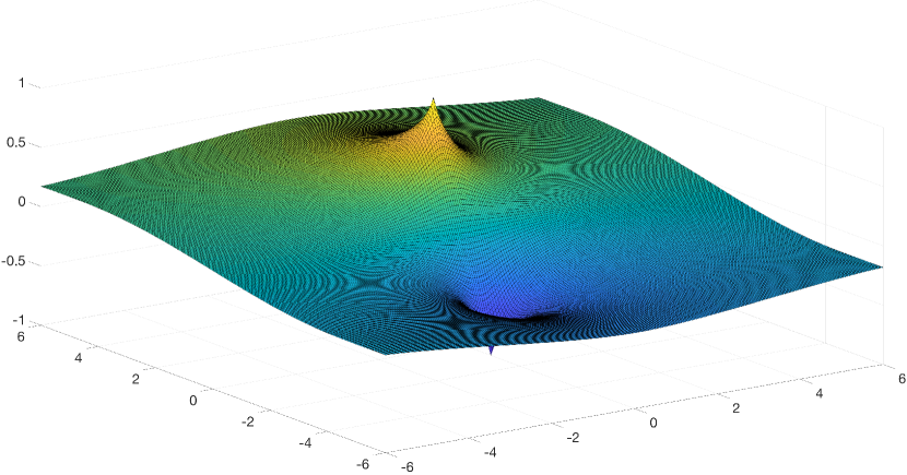
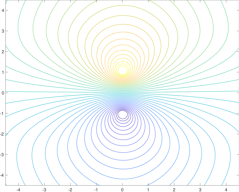
Equation (1.3) can be used to show that each extremal is bounded and has various symmetry properties. In this note, we will make use of these facts to prove the following theorem. We interpret the existence of limit (1.6) below as asserting that extremals are asymptotically flat. This result was also confirmed by numerical computations as observed in Figure 1.
Theorem 1.1.
Suppose and that . If is an extremal which satisfies (1.2), then
| (1.6) |
and
| (1.7) |
Furthermore,
| (1.8) |
is nonincreasing in for some and tends to as .
In proving Theorem 1.1, we will first verify that any bounded -harmonic function on the exterior domain
is asymptotically flat for . That is, there is some for which
By employing a Harnack inequality, we can quantify this assertion and show there are positive numbers and such that
| (1.9) |
In particular, we will be able to conclude that the limit (1.6) occurs with an (at least) algebraic rate of convergence.
The precise decay estimate we derive is described as follows.
Theorem 1.2.
Suppose and . There are positive constants and such that
for each function that is bounded and -harmonic in .
Then we’ll show how these results extend to solutions of the multipole equation
| (1.10) |
where are distinct and satisfy . The main point is to establish that each solution is bounded. Moreover, we will argue that each solution is not differentiable at any in which it has a strict local maximum or minimum. Finally, in the appendix, we will explain the numerical method we used to produce Figure 1 as shown above.
2 Bounded -harmonic functions on exterior domains
In what follows, we will suppose that
are fixed. Even though we are primarily interested in functions defined on , we will also consider functions defined on bounded domains or possibly on the complement of such subsets. Recall that each function in the Sobolev space has a Hölder continuous representative (Theorem 5 section 5.6 of [3]). Consequently, we will always identify a function with its continuous representative and consider as a subset of the continuous functions on .
For a given domain , we will say that is -harmonic in and write
so long as and
| (2.1) |
for each . Likewise, for a signed Borel measure on , we say that
provided and
| (2.2) |
for all .
In this section, we will establish three facts about bounded -harmonic functions on . We first show that these functions are all asymptotically flat and their gradients tend to zero as at a certain rate. Then we show that if one of these functions lies strictly between two values, its limit as lies strictly between these two values, as well. Finally, we establish decay and monotonicity properties of two integral quantities involving these functions.
2.1 Asymptotic flatness
As mentioned above, our first order of business is to verify the asymptotic flatness of bounded -harmonic functions on . This is the central goal of this subsection. We also note that the first part of following statement has essentially been verified by Serrin [15], who showed that a positive -harmonic function on an exterior domain has a positive limit as or tends to at a specific rate; this result was also extended recently by Fraas and Pinchover [4, 5]. Our result is not as general, however our proof is simple and direct.
Proposition 2.1.
Suppose is a bounded -harmonic function on . Then the limit
exists and
To this end, we will need to make use of a version of Caccioppoli’s inequality and a Liouville-type assertion for -harmonic functions on punctured domains.
Lemma 2.2.
Suppose is a domain and . Further assume satisfies
| (2.3) |
in for some constant . Then for each nonnegative ,
| (2.4) |
Proof.
Corollary 2.3.
Suppose is a domain and . Further assume satisfies
| (2.5) |
in for some constant . Then
| (2.6) |
Proof.
Choose with , in and
Then set
Clearly, is nonnegative, in and
The conclusion follows from substituting this in (2.4). ∎
Corollary 2.4.
Suppose is bounded and satisfies
| (2.7) |
in for some constant . Then is necessarily constant and .
Proof.
We are now ready to employ these observations to fashion a proof of Proposition 2.1.
Proof of Proposition 2.1.
1. For , set
| (2.8) |
Note that is -harmonic on . Without loss of generality, suppose for all , so that
for . We will now proceed to send .
By a result of Ural’ceva [17] (see also Lewis [10] and Evans [2]), there is depending on and such that
for each compact and sufficiently large. Here depends on and and . Consequently, there is a sequence with and such that
| (2.9) |
for each compact . It follows easily that is -harmonic on .
By Theorem 1.1 and Remark 1.6 of [8] (see also [9]), there is a constant such that
| (2.10) |
in . Moreover,
This limit gives that is locally integrable in a neighborhood of . Since
for all , we have . Corollary 2.4 then implies that is identically equal to a constant and so
locally uniformly on .
2. Consider
for . By the comparison principle for -harmonic functions,
for . It follows that
for . In particular, is quasiconcave. So there is for which is monotone (Theorem 17 in Chapter 3 of [12]) and thus
exists.
We can choose an with so that
We may as well also suppose that is convergent. In this case,
With virtually the same argument, we find
Consequently,
uniformly for .
3. Now let be a sequence such that . Without loss of generality, we will suppose and that is convergent as these properties are true for a subsequence of . Then
and we conclude that
We also have that
tends to uniformly for . Choosing as above, we find
That is,
∎
Remark 2.5.
This theorem can be proved without appealing to the estimates for -harmonic functions. Local uniform convergence of a subsequence of in would follow from Morrey’s inequality, and convergence in can be verified using the Browder and Minty method (as described in section 9.1 of [3]).
Remark 2.6.
In Corollary 4.2 below, we will show that is nondecreasing and is nonincreasing for all .
2.2 Strict bounds on limiting values
The next assertion states that the limit of a bounded -harmonic function on always lies strictly within the bounds observed by the function. In particular, any bounded and positive -harmonic function on an exterior domain has a positive limit. Pinchover and Tintarev [13] established this conclusion using a different argument and for more general operators.
Proposition 2.7.
Suppose is -harmonic in and
for some . Then
| (2.11) |
Proof.
Fix , and for define
Note that is -harmonic in the annulus ,
Now choose such that
By comparison,
| (2.12) |
Let and suppose . Then and so
| (2.13) | ||||
| (2.14) | ||||
| (2.15) |
As a result,
Likewise, we find . ∎
Remark 2.8.
We will see in Corollary 4.2, that the same conclusion holds only assuming
for some . This improvement relies on a global comparison property of bounded -harmonic functions on the exterior domain .
2.3 Integral decay and monotonicity
In Proposition 2.1, we showed that if is a bounded -harmonic function in , then
| (2.16) |
This limit immediately implies the following decay property.
Corollary 2.9.
Suppose is bounded and -harmonic in . Then
| (2.17) |
for any . Moreover,
| (2.18) |
Proof.
Fix . By (2.16), there is so large that
for . Then
Since
the first assertion follows. As for the second claim,
The conclusion follows as is arbitrary. ∎
Using a certain identity for smooth -harmonic functions, we can strengthen the conclusion of the previous corollary.
Proposition 2.10.
Suppose is smooth, bounded and -harmonic in . Then
| (2.19) |
is nonincreasing. In particular,
| (2.20) |
Moreover,
| (2.21) |
for each .
3 Asymptotics of extremals
This section is dedicated to the proof of Theorem 1.1. Let be an extremal satisfying (1.2). In Proposition 3.5 of [6], we established that
| (3.1) |
for each ; this inequality is also established in Lemma 5.4 below. As a result, is uniformly bounded and is -harmonic in for
It follows from Proposition 2.1 that the limit
exists and
As is smooth in (section 4.3 of [6]), we can apply Proposition 2.10 to conclude
for . Moreover, this quantity is nonincreasing on and tends to as .
In Proposition 3.4 of [6], we showed
for each . This equality implies that is antisymmetric with respect to reflection about the hyperplane
In particular,
for each . As is unbounded, it must be that
4 Quantitative flatness
We will now establish a Harnack inequality for bounded, nonnegative -harmonic functions on . We will then prove Theorem 1.2 similar to how Hölder continuity of -harmonic functions can be established with a Harnack inequality (as explained in section 2 of [11]). To this end, we will start with the following comparison principle.
Lemma 4.1.
Suppose and that are bounded and -harmonic in with
on . Then
in .
Proof.
In view of the monotonicity of the mapping ,
| (4.1) | ||||
| (4.2) |
As is bounded and vanishes on , we can integrate by parts and appeal to (2.16) in order to deduce
| (4.3) | ||||
| (4.4) | ||||
| (4.5) | ||||
| (4.6) | ||||
| (4.7) |
Combining with (4.1) gives
As is strictly monotone, it must either be that the Lebesgue measure of is zero or that almost everywhere in . If the Lebesgue measure of is zero, for almost every ; as are continuous, this would imply that for every . Otherwise, in which would mean is constant throughout Since vanishes on , we would have in . That is, in . ∎
Corollary 4.2.
Suppose is -harmonic and bounded in .
-
(i)
For each ,
-
(ii)
For ,
-
(iii)
For ,
-
(iv)
If and for , then
Proof.
We will only prove the statements involving suprema. Let denote the constant function on which is equal to . As is bounded, -harmonic, and for , it follows that for each . That is,
By part ,
Part also implies
Choose so small that . By part , for each . Consequently, . ∎
The following harnack inequality is now an easy consequence of these observations.
Proposition 4.3.
There is a constant such that
| (4.8) |
for each and bounded, nonnegative -harmonic in .
Remark 4.4.
The example shows that the boundedness assumption cannot be removed.
Proof.
Along with this Harnack inequality, we will need one more fact to prove Theorem 1.2.
Lemma 4.5.
Suppose is nonincreasing and satisfies
for some . Then
for .
Remark 4.6.
, so decays like a power of as .
Proof.
By induction,
for each nonnegative integer . Choose so that
and
Then
∎
Proof of Theorem 1.2.
Set
for . Observe that and are nonincreasing. Also note is a bounded, nonnegative -harmonic function for . By Proposition 4.8,
for some independent of . Likewise is a bounded, nonnegative -harmonic function for , so
Adding these inequalities gives
That is,
By the Lemma 4.5,
for some ; here we used . In particular,
for . ∎
Corollary 4.7.
5 Multipole equation
We define
| (5.1) |
and suppose are distinct and are given. Let us consider the minimization problem: find which minimizes the integral
| (5.2) |
subject to the constraints
| (5.3) |
Direct methods from the calculus of variations can be used to show that there is a minimizer . Moreover, as the Dirichlet integral (5.2) is strictly convex, is unique.
These observations were first noted by Kichenassamy in section 2.3 of [7]. Discrete analogs of this minimization problem also arise in semi-supervised learning with labels as studied recently by Calder [1] and by Slepčev and Thorpe [16]. We became interested in this problem when we noticed that the minimizer above satisfies a generalized version of the PDE solved by Morrey extremals.
Proposition 5.1.
Remark 5.2.
Choosing in (5.4), we see that .
Remark 5.3.
If satisfies (5.4), then is a solution of the multipole equation
| (5.5) |
Proof.
It also turns out that minimizers are uniformly bounded.
Lemma 5.4.
Proof.
We will only establish the claimed upper bounds. Set
and define
It is plain to see that and that satisfies (5.3). Moreover,
Observe that is nonpositive and -harmonic in the domain . By the strong maximum principle (Corollary 2.21 of [11]), it is either that or in . Since is not constant in is must be that in . ∎
Corollary 5.5.
Remark 5.6.
We can also make a few basic observations about a particular level set of solutions of equation (5.5).
Corollary 5.7.
Proof.
We have established
Since is continuous, there is some for which . Consequently, .
If for some , then either in or in . If in , then is a bounded and positive -harmonic function on an exterior domain. By Proposition 2.7, there is a such that as . However, this contradicts as . Thus, no such exists and is noncompact.
Finally, we note that if there is a sequence with and then
That is, is compact when . ∎
Remark 5.8.
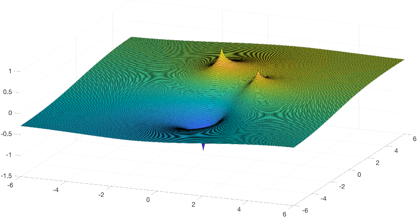
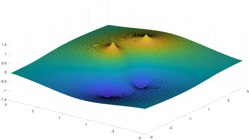
We conclude by studying the (non)differentiability of minimizers at the points . This and the other properties we have already discussed about solutions of the multipole PDE may be seen in Figures 3 and 4.
Proposition 5.9.
Proof.
We will prove that is not differentiable at provided that it has a strict local max at . With this assumption, there is some such that for . In particular,
| (5.12) |
Choosing smaller if necessary, we may also suppose that is -harmonic in .
Set
for . Note that and
As is -harmonic in , comparison gives in .
If is differentiable at , then
| (5.13) | ||||
| (5.14) | ||||
| (5.15) | ||||
| (5.16) |
as . Rearranging this inequality gives
And sending leads us to
which contradicts (5.12). Consequently, is not differentiable at . ∎
Corollary 5.10.
Appendix A Numerical method
We will now discuss the method used to approximate the solution of PDE (1.3) displayed in Figure 1. It turns out that this method also can be adapted to obtain approximations of solutions of the multipole equation (5.5), as exhibited in Figures 3 and 4. For simplicity, we will focus on the particular case of approximating a solution of the PDE
| (A.1) |
in . We will also change notation and use ordered pairs to denote points in so that .
Observe that any solution of (A.1) minimizes
| (A.2) |
among all . For a given , we may also consider the problem of minimizing
| (A.3) |
amongst . It is not hard to show this problem has a minimizer . Further, it is routine to check that converges to for each as , where is the unique minimizer of (A.2) with . Consequently, we will focus on approximating .
Below we will show how to derive a discrete version of our minimization problem for . Then we will explain how to use an iteration scheme based on a quasi-Newton method. Again we emphasize that all of the figures in this article were based on this method or minor variants to account for differences in the particular examples we considered.
A.1 Discrete energy
Let us fix () and discretize the interval along the -axis with
for . Here
and we note that each of the subintervals has length . We can do the same for the interval along the -axis and obtain
for . Our goal is to derive an appropriate energy specified for functions defined on the grid points .
To this end, we observe that if is sufficiently smooth
We also suppose for some which gives
and
As a result, we will attempt to minimize
| (A.4) |
over the variables
A minimizer for would then form an approximation for on the grid points
A.2 Quasi-Newton method
We used a multidimensional version of the secant method to approximate minimizers of the discrete energy defined above in (A.4). In particular, since is convex we only need to approximate a such that
for each with .
First we chose the initial guesses
and
Here
is approximately equal to
which is a solution of the Dipole equation in .
Then we performed the iteration
| (A.5) |
for until the stopping criterion
was achieved. The iteration was computed for all except for .
References
- [1] Jeff Calder. The game theoretic -Laplacian and semi-supervised learning with few labels. Nonlinearity, 32(1):301–330, 2019.
- [2] Lawrence C. Evans. A new proof of local regularity for solutions of certain degenerate elliptic p.d.e. J. Differential Equations, 45(3):356–373, 1982.
- [3] Lawrence C. Evans. Partial differential equations, volume 19 of Graduate Studies in Mathematics. American Mathematical Society, Providence, RI, second edition, 2010.
- [4] Martin Fraas and Yehuda Pinchover. Positive Liouville theorems and asymptotic behavior for -Laplacian type elliptic equations with a Fuchsian potential. Confluentes Math., 3(2):291–323, 2011.
- [5] Martin Fraas and Yehuda Pinchover. Isolated singularities of positive solutions of -Laplacian type equations in . J. Differential Equations, 254(3):1097–1119, 2013.
- [6] Ryan Hynd and Francis Seuffert. Extremals of Morrey’s inequality. Preprint, 2018.
- [7] Satyanad Kichenassamy. Quasilinear problems with singularities. Manuscripta Math., 57(3):281–313, 1987.
- [8] Satyanad Kichenassamy and Laurent Véron. Singular solutions of the -Laplace equation. Math. Ann., 275(4):599–615, 1986.
- [9] Satyanad Kichenassamy and Laurent Véron. Erratum: “Singular solutions of the -Laplace equation”. Math. Ann., 277(2):352, 1987.
- [10] John L. Lewis. Regularity of the derivatives of solutions to certain degenerate elliptic equations. Indiana Univ. Math. J., 32(6):849–858, 1983.
- [11] Peter Lindqvist. Notes on the -Laplace equation, volume 102 of Report. University of Jyväskylä Department of Mathematics and Statistics. University of Jyväskylä, Jyväskylä, 2006.
- [12] Béla Martos. Nonlinear programming. North-Holland Publishing Co., Amsterdam-Oxford; American Elsevier Publishing Co., Inc., New York, 1975. Theory and methods.
- [13] Yehuda Pinchover and Kyril Tintarev. On positive solutions of minimal growth for singular -Laplacian with potential term. Adv. Nonlinear Stud., 8(2):213–234, 2008.
- [14] James Serrin. Local behavior of solutions of quasi-linear equations. Acta Math., 111:247–302, 1964.
- [15] James Serrin. Singularities of solutions of nonlinear equations. In Proc. Sympos. Appl. Math., Vol. XVII, pages 68–88. Amer. Math. Soc., Providence, R.I., 1965.
- [16] Dejan Slepčev and Matthew Thorpe. Analysis of -Laplacian regularization in semisupervised learning. SIAM J. Math. Anal., 51(3):2085–2120, 2019.
- [17] N. N. Ural’ceva. Degenerate quasilinear elliptic systems. Zap. Naučn. Sem. Leningrad. Otdel. Mat. Inst. Steklov. (LOMI), 7:184–222, 1968.