CO Emission in Infrared-Selected Active Galactic Nuclei
Abstract
In order to better understand how active galactic nuclei (AGN) effect the interstellar media of their host galaxies, we perform a meta-analysis of the CO emission for a sample of galaxies from the literature with existing CO detections and well-constrained AGN contributions to the infrared (67 galaxies). Using either Spitzer/IRS mid-IR spectroscopy or Spitzer+Herschel colors we determine the fraction of the infrared luminosity in each galaxy that can be attributed to heating by the AGN or stars. We calculate new average CO spectral line ratios (primarily from Carilli & Walter 2013) to uniformly scale the higher- CO detections to the ground state and accurately determine our sample’s molecular gas masses. We do not find significant differences in the gas depletion timescales/star formation efficiencies (SFEs) as a function of the mid-infrared AGN strength ( or ), which indicates that the presence of an IR-bright AGN is not a sufficient sign-post of galaxy quenching. We also find that the dust-to-gas ratio is consistent for all sources, regardless of AGN emission, redshift, or , indicating that dust is likely a reliable tracer of gas mass for massive dusty galaxies (albeit with a large degree of scatter). Lastly, if we classify galaxies as either AGN or star formation dominated, we do not find a robust statistically significant difference between their CO excitation.
1. Introduction
The production of luminous quasars is a dramatic story, wherein two immense galaxies collide, fueling a burst of star formation and triggering rapid growth of a supermassive black hole (e.g., Sanders & Mirabel, 1996; Hopkins et al., 2006; Goulding et al., 2018). In this scenario, the active galactic nucleus (AGN) goes through an obscured growth phase, where the accretion disk is hidden by a dust torus. This phase ends when the AGN launches winds powerful enough to blow away some of the circumnuclear obscuring dust so that the accretion disk becomes visible in the optical (Glikman et al., 2012). As the winds clear away the circumnuclear dust, the galaxy’s star formation quenches due to galaxy-scale, AGN-driven outflows (Page et al., 2012; Pontzen et al., 2017). However, evidence for this scenario is strongly linked to observational biases. In large statistical samples of optically-selected AGN (Stanley et al., 2017) and X-ray+IR selected AGN (Harrison et al., 2012), no correlation between AGN luminosity and decreased star formation rate is observed. On the other hand, theoretical models suggest AGN may occur at a special phase in a galaxy’s life, immediately prior to quenching (Caplar et al., 2018). X-ray selected AGN at are observed to occur after a galaxy has compactified and but before star formation decreases in the center of the galaxy (Kocevski et al., 2017).
At , galaxies both on and above the “main sequence” (e.g., Brinchmann et al., 2004; Daddi et al., 2007; Elbaz et al., 2007; Noeske et al., 2007) appear to have higher gas masses, gas mass fractions, and star formation rates than local galaxies (e.g., Tacconi et al., 2013; Scoville et al., 2016). The high star formation rates (SFRs) and gas masses of dusty galaxies are a particular challenge for simulation work, both in terms of reproducing the characteristics of these high- systems and in terms of the resulting “red and dead” galaxy populations that would exist today (e.g., Casey et al. 2014 and references therein; though see Narayanan et al. 2015). Given the tight correlation observed between galaxies’ black hole masses and bulge masses at (implied by the - relation; Ferrarese & Merritt 2000; Gebhardt et al. 2000) and the concurrent peaks of both AGN and star formation activity at , theoretical studies have suggested that AGN may play a role in quenching the high SFRs of massive galaxies in the early universe (e.g., Somerville et al., 2008).
However, AGN may not be solely responsible for quenching star formation. Recently, Spilker et al. (2018) found molecular mass outflow rates a factor of two higher than the SFR in a star forming galaxy at that lacked an AGN. In contrast, Hunt et al. (2018) find a quenched galaxy at with a large molecular gas reservoir and no indication of gas outflows. Indeed, post-starburst galaxies, which lack AGN signatures, are seen to retain large molecular gas reservoirs (albeit with depleted dense gas; French et al. 2015; Suess et al. 2017; French et al. 2018). How these results fit with growing supermassive black holes into a quenching paradigm remains unclear. Both the relative importance of AGN feedback to stellar feedback (e.g., Bouché et al., 2010; Davé et al., 2011; Shetty & Ostriker, 2012; Lilly et al., 2013; Kim et al., 2013) and exact feedback mechanism for AGN (outflows vs. accretion suppression; e.g., Croton et al. 2006; Hopkins et al. 2006; Gabor et al. 2011; Cicone et al. 2014) are still debated. In addition, recent work suggests that AGN may locally enhance star formation (e.g., Stacey et al., 2010; Ishibashi & Fabian, 2012; Silk, 2013; Mahoro et al., 2017).
While the influence of AGN on galaxy-wide scales is unclear, AGN are known to heat their torus and circumnuclear dust to K, producing an IR SED that emits as a power-law in the near and mid-IR (Elvis et al., 1994). Empirically, dust-enshrouded AGN are observed to heat circumnuclear dust out to at least 40 m, producing a flattening in the far-IR (Mullaney et al., 2011; Sajina et al., 2012; Kirkpatrick et al., 2012; Symeonidis et al., 2016; Ricci et al., 2017). Physical radiative transfer models of the narrow line region (NLR) also predict a modified blackbody peaking at m from dust clouds comingled with the ionized gas (Groves et al., 2006). AGN may therefore have a non-negligible contribution to the infrared luminosity () and thus any inferred IR SFRs if the AGN is not properly accounted for. The far-IR influence of AGN produces an enhanced dust emission with temperatures of 100 K (Kirkpatrick et al., 2012). Gas and dust are largely considered to be comingled within the interstellar medium, at least locally, implying that AGN could be heating the molecular reservoirs in the centers of galaxies as well, producing a possible feedback mechanism that does not require outflows. However, at , gas fractions have dramatically increased, and there has been some suggestion that the gas reservoirs are more spatially extended than the dust (e.g., Hodge et al. 2015, 2016; Tadaki et al. 2017 but see also Hodge et al. 2018).
If AGN influence the star formation history of galaxies, their effects may be measured in the molecular ISM that fuels star formation. Molecular outflows have been observed in the CO rotational lines of luminous Type 1 and Type 2 QSOs at low redshift (e.g., Feruglio et al., 2010; Cicone et al., 2014; Fiore et al., 2017), but outflows are not present in all AGN host galaxies. Very high excitation CO lines () have been observed in some AGN at all redshifts (e.g., Weiß et al., 2007; Ao et al., 2008; Hailey-Dunsheath et al., 2012; Spinoglio et al., 2012; Rosenberg et al., 2015), but this component likely represents a small fraction of their total molecular gas reservoirs. At high redshift, the CO spectral line energy distributions (SLEDs) of Type 1 QSOs are known to peak, on average, at higher- transitions () than those of star-forming submillimeter-selected galaxies (SMGs; ; e.g., Weiss et al. 2007; Carilli & Walter 2013). However, when high star formation rate densities can explain SLED excitation (e.g., Narayanan & Krumholz, 2014) it is challenging to isolate the potential effects of the AGN in driving these more moderate excitation CO rotational lines.
In this paper, we reanalyze data from the literature to examine whether AGN that are heating circumnuclear dust may also affect the molecular ISM. In our reanalysis, we demonstrate how different measurements of infrared luminosity and AGN heating can cause incongruent conclusions about the state of the ISM in AGN. In Section 2, we discuss our sample selection. In Section 3, we describe how we assess the presence and strength of obscured AGN, determine and the inferred SFRs, and use new average SLEDs from the literature to calibrate the gas masses of our sample. In Section 4, we look for evidence of decreased star formation efficiency in AGN and evaluate CO SLEDs for effects from the central AGNs. Finally, in Section 5, we summarize and lay out future directions for uncovering the true effect of an AGN on its host ISM.
2. Sample Selection
We aim to compare the CO emission properties of IR-selected AGN with star forming galaxies. Due to the lack of a homogeneous survey, we reanalyze published sources. This technique has also been employed by other authors due to the difficulty of carrying out large scale molecular gas surveys (e.g. Herrera-Camus et al., 2019; Perna et al., 2018). The meta-analysis necessarily means that our sample will be heterogeneous, although we apply the same analysis techniques uniformly to each source. The relatively recent Carilli & Walter (2013) annual review described molecular gas in galaxies at . This review compiled 173 galaxies with spectroscopic redshifts where molecular gas had been measured, comprising all published measurements at that time. From this parent sample, we initially selected all galaxies with a CO line flux for any transition, that have a magnification , and with at least 3 photometric data points spanning the range m. We also removed two galaxies (SMM J105131 and SMM J09431+4700) since they are resolved doubles in their CO emission, but we do not have matching resolved mid-IR colors or IRS spectroscopy to disentangle the AGN emission from the two sources.111SMM J123707+6214 is also a resolved double. However, the combined system has a measured mid-IR AGN fraction of , so we do not have to worry about differences in the two components’ AGN fractions. In addition, the CO line ratios are identical between the two components (Riechers et al., 2011b), so we can treat the system as one for our analysis without any biasing concerns (this effectively under-weights SMM J123707+6214). We also add in three 70 m selected galaxies (GN70.38, GN70.8, GN70.104) from Pope et al. (2013), where CO was observed with IRAM/PdBI; these galaxies were not in the Carilli & Walter (2013) compilation. We add in three more QSOs (COB011, no.226, 3C 298) from the Perna et al. (2018) compilation which meet our criteria for full coverage of the IR SED. Additionally, we include 10 galaxies at from Kirkpatrick et al. (2014), which have CO(1-0) measured with the Large Millimeter Telescope, have Herschel observations covering the far-IR, and have Spitzer mid-IR spectroscopy. We have a total heterogenous sample of 67 galaxies. Figure 1 shows the redshift- distribution of our final sample of 67 galaxies. We list all sources, redshifts, and in Table 3 in the Appendix.
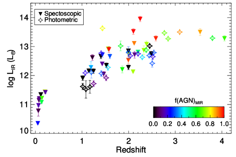
The triangles indicate galaxies where we identified IR AGN using Spitzer mid-IR spectroscopy, while the stars are galaxies where AGN were found using IR color diagnostics.
3. Methods: AGN fraction, SFR, , and
3.1. AGN fractions from Spitzer Spectroscopy and IR Colors
We use either Spitzer IRS spectroscopy (available for 41 galaxies) or IR color diagnostics (26 galaxies) to locate AGN within our sample. We quantify , the fraction of mid-IR (m) luminosity arising from an AGN torus. We do not perform a full SED decomposition into multiple components as has become common in the literature because this risks overfitting and overinterpretting the sparse amount of IR data available.
The low resolution () Spitzer IRS spectra were reduced following the method outlined in Pope et al. (2008). We used the Spitzer IRS spectra to calculate the AGN contribution to the mid-IR luminosity following the technique described in Pope et al. (2008) and Kirkpatrick et al. (2015). We fit the individual spectra with a model comprised of three components: (1) the star formation component is represented by the mid-IR spectrum of the prototypical starburst M 82; (2) the AGN component is determined by fitting a pure power-law with the slope and normalization as free parameters; (3) an extinction curve from the Draine (2003) dust models is applied to the AGN component; for our wavelength range, the extinction curve primarily constrains the 9.7 m silicate absorption feature. We fit all three components simultaneously. We integrate under the best fit model and the power-law component to measure . Our spectroscopic measurement technique is uncertain by less than 10% in (Kirkpatrick et al., 2015).
For the 26 sources that lack mid-IR spectroscopy, we determine using Spitzer+Herschel color classification as described in Kirkpatrick et al. (2017), which is based on observed AGN emission in galaxies at . We created a redshift dependent diagnostic that assigns an depending on the ratio of , which at separates AGN on the basis of a hot torus as compared with the 1.6 m stellar bump seen in star-forming galaxies (SFGs). This is combined with either or , which trace the relative amounts of cold and hot dust (since AGN should have a larger hot dust component). Color determination of in this manner is accurate to 30% (Kirkpatrick et al., 2017).
Our mid-IR classifications largely agree with the classifications in Carilli & Walter (2013). That is, sources with are predominately listed as a type of star forming galaxy in Carilli & Walter (2013), and the radio AGN and QSOs identified in Carilli & Walter (2013) all have . In addition, we identify 9 additional galaxies as AGN that were originally listed as star forming galaxies in Carilli & Walter (2013). We note our 9 “new” AGN in Table 3.
3.2. and SFRs
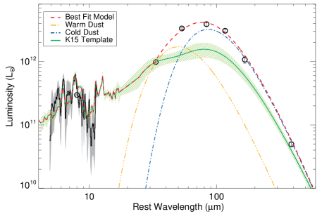
We gathered all available photometry for our sample using the Spitzer/IRSA and NED databases. The number of far-IR data points per source varies. To allow the greatest flexibility when determining , we combine a template from Kirkpatrick et al. (2015), which are empirically derived from galaxies at , with a far-IR model consisting of two modified blackbodies. The number of data points at m determines how many far-IR parameters we allow to vary, so that we are at most fitting for parameters. At a minimum, we only fit for the normalization of the cold component, and a maximum, we fit both normalizations and the cold dust temperature. The warm dust temperature is held fixed at 65-90 K, where using a warmer dust temperature depends on the presence of an AGN (Kirkpatrick et al., 2012). Here, we use a warmer dust temperature when , which is when this component starts to contribute measurably () to the far-IR SED (Kirkpatrick et al., 2015). We choose this simple method rather than using a library of models because we do not want to risk over-fitting a scarcity of data points in many sources. As we are not trying to measure dust temperatures or , we are not concerned with degeneracies between the parameters. is robust against small variations in and as long as the model fits all the data points. The Kirkpatrick et al. (2015) library provides templates based on , and we use the appropriate template for each source to complete the best fit model at m. In Figure 2 we illustrate how our technique of modifying templates is more accurate than simply scaling a template to a photometric data point.
The can be converted to a SFR once the AGN heating is removed. Due to the disparate data available for each source, we are not able to decompose the full SEDs into an AGN and star forming component. However Kirkpatrick et al. (2015) demonstrate that is related to , the AGN contribution to m), through the quadratic relation
| (1) |
We correct for AGN heating using using
| (2) |
and then convert to a SFR following Murphy et al. (2011):
| (3) |
3.3. Dust Masses
In order to explore whether increased AGN heating of the ISM affects the gas-to-dust ratio in galaxies, we use two methods for determining the dust mass in our sample.
For the first method, we calculate the dust mass and characteristic radius of the dust emission using the physically motivated, self-consistent radiative transfer model from Chakrabarti & McKee (2005, 2008). The far-IR SED can be characterized by the ratio of to and the radius of the source for a given dust opacity (Witt & Gordon, 2000; Misselt et al., 2001; Chakrabarti & McKee, 2005, 2008). The authors use the Weingartner & Draine (2001) dust models with to parameterize the grain composition and emission properties. It should be noted that the choice of has a negligible effect in the far-IR, where is calculated. The authors make the simplifying assumption that star forming regions can be represented as homogeneous and spherically symmetric. Each star forming region is surrounded by spherical shells of dust, and the temperature and density profiles of the dust shells are approximated as power-laws. The radiative transfer code also calculates a far-IR luminosity (m), which is consistent with our calculated above. Many of our galaxies lack enough data to fit the near, mid, and far-IR with a robust dust model (such as Draine & Li, 2007) that calculates grain populations. As the relative abundance of small grains and carbonaceous grains does not have a significant effect on the large-grain submm emission, we opt for a model that only fits the far-IR. We list and from the Chakrabarti & McKee (2005) model in Table 4.
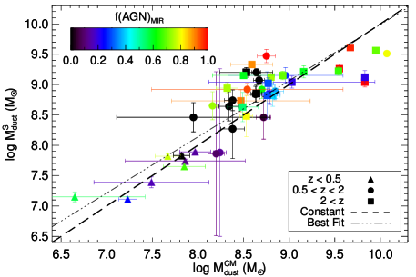
For comparison to the Chakrabarti & McKee (2005) model, we also calculate the dust mass using the simple model of Scoville et al. (2016). In this model, the dust mass is calculated using any sub-mm observation with m, and assuming a standard cold dust temperature of 25 K. Several of our galaxies lack a sub-mm observation at m, so we are unable to calculate a dust mass in this manner. We compare these dust masses, and , in Figure 3; their values are broadly consistent. The large errors on many indicate the unreliability of fitting a multi-component model to a scarce number of data points. Some of our galaxies only had two photometric measurements beyond m.
3.4. and Gas Masses
3.4.1 Excitation Correction
Our sample have been observed in many different CO lines. In order to determine and the associated gas masses free from excitation effects, assumptions need to be made about the line ratios in objects that do not have measurements of the CO(1–0) line (the ground-state rotational transition that best traces the total molecular gas). Bothwell et al. (2013) produced an average CO spectral line energy distribution (SLED) for a sample of – SMGs with spectroscopic redshifts (generally from Lyman-, , or PAH observations). However, there are significantly more CO detections currently in the literature, particularly more objects with CO(1–0) detections and more objects at higher redshifts.
We therefore construct a new average CO SLED using the entire library of high- CO detections from Carilli & Walter (2013), supplemented with new CO detections from Pope et al. (2013), Aravena et al. (2014), Sharon et al. (2016), Yang et al. (2017), Frayer et al. (2018), Perna et al. (2018) and references therein. We have included the entire library, as opposed to just those sources with well-sampled IR SEDs, in order to make use of all the available molecular gas information and therefore reduce uncertainties on our new SLED.
To construct the average CO SLED, we follow Bothwell et al. (2013). We linearly scale all sources’ line fluxes and uncertainties by the ratio of their FIR luminosity to the approximate median FIR luminosity of the full sample () in order to prevent the brightest sources from biasing later averages. For each CO transition, we find the median scaled line luminosity for all sources detected in that line. We determine the uncertainty on the median scaled line luminosity via bootstrapping (with replacement) over 10,000 iterations, perturbing the random subset of line fluxes by their uncertainties in each iteration. We note that many sources from Carilli & Walter (2013) have small uncertainties. We assume that if those uncertainties are less than of the measured value, then only the statistical uncertainty was reported. For those objects, we add an additional uncertainty in quadrature to the reported value in order to approximate flux calibration uncertainties. For the very few line measurements with missing uncertainties, we assume a uncertainty. Note that this analysis only includes reported line detections, which may produce a median SLED biased both towards the characteristics of the brighter classes of objects that are more commonly observed (which cannot be accounted for by luminosity scaling) and towards higher-excitation specifically (since upper limits from higher- non-detections are not included in the analysis).
We give the ratio of the median line luminosity to the median CO(1–0) line luminosity (using the scaled measured values) and the standard deviation of the ratio (from bootstrapping) in Table 1. The line ratios (in units of brightness temperature) can be related to the line luminosity and integrated line flux by
| (4) |
In Figure 4, we plot the median CO SLED, as well as the individual line ratios contributing to that SLED. For individual sources that lack CO(1–0) measurements, we use the median CO(1–0) flux from our bootstrapped analysis, scaled by the ratio of that source’s FIR luminosity to the fiducial value, in order to calculate and plot an illustrative line ratio for that object.
| Measured Sample | ||||||||||||
|---|---|---|---|---|---|---|---|---|---|---|---|---|
| All Sources | Matched , , | All | IRS-determined | Color-determined | ||||||||
| Transition | Ratio | Ratio | Ratio | RatioaaThe astute reader may notice that combined median ratios do not always fall between the color-determined and IRS-determined median ratios (similar effects are also seen for other ratios presented in this paper). This result is due to our method of calculating a ratio of medians as opposed to a median of ratios as described in Section 3.4.1 (which is necessary since not all sources have detections of both the relevant lines and we want to use all available information). Since we calculate the median and the median , those luminosities may skew in different directions depending on the number of detections and luminosities of their sub-populations. Thus the resulting ratio of median luminosities may be higher or lower than that of the objects or sub-samples from which the ratio is composed. | Ratio | Ratio | ||||||
| CO(1–0) | ||||||||||||
Note. — The first three sets of median line ratios are calculated from the parent sample of Carilli & Walter (2013), Pope et al. (2013), Aravena et al. (2014), Sharon et al. (2016), Yang et al. (2017), Frayer et al. (2018), Perna et al. (2018) and references therein (which includes our sample with calculated mid-IR AGN fractions), and various subsets as indicated by the columns’ titles. Median line ratios for our sample with measured mid-IR AGN fractions are shown in the last three columns. In all cases, refers to the number of galaxies with detections of the specified CO transition that contribute to the median line luminosity, and thus the median line ratio.
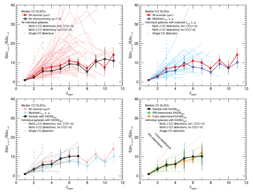
Many high- sources studied in CO are gravitationally lensed due to the advantageous boosting of the observed flux. However, spatially varying magnification factors may interact with spatially varying properties of the galaxy, biasing unresolved measurements of lensed galaxies’ fluxes (e.g., Blain, 1999; Hezaveh et al., 2012; Serjeant, 2012). In a series of simulations, Serjeant (2012) showed that differential lensing tends to scatter unresolved measurements of galaxies’ average properties towards those of their most compact and luminous regions (like those of the central AGN and star-forming clouds, which are typically warmer than the ambient material), particularly for strongly lensed sources with magnifications of . Since differential lensing could bias measured CO SLEDs towards more high- CO emission, we also compute the median CO SLED as above, but restrict the included sources to those with magnifications of , where Serjeant (2012) found little evidence for differential lensing affecting the shape of galaxy-wide average CO SLEDs (Figure 4, top left). This selection reduces the number of lines in the sample by . While removing the strongly-lensed sources does systematically produce lower line ratios (at least where there are a significant number of input line measurements), differences in individual line ratios are not statistically significant (Table 1).
Galaxies’ observed CO SLEDs can also be affected by the cosmic microwave background (CMB), which can both act as an additional heating mechanism and as a background above which the CO lines must be detected (e.g., da Cunha et al., 2013, and references therein). For galaxies at higher redshifts (), da Cunha et al. (2013) finds that the CMB’s effect on theoretical CO SLEDs can be substantial. However, the effects on the measured line ratios also depend on the density and temperature of the molecular gas. We therefore cannot apply redshift-dependent corrections to individual galaxies in our sample since we do not have a priori constraints on their gas physical conditions. Therefore, our redshift-binned samples will have some additional scatter introduced by the effects of the CMB. However, the effects of the CMB in the redshift range of interest () are generally much smaller than the scatter introduced by the galaxies’ intrinsic range of gas temperatures and densities (da Cunha et al., 2013).
To ensure that including such a broad range of redshifts and IR luminosities will not bias our updated SLED, we also calculate the median line ratios for the sub-sample of galaxies from Carilli & Walter (2013), Perna et al. (2018), etc. that matches the redshift (), magnification (), and IR luminosity () of our mid-IR sample described in Section 2. The median CO line ratios are reported in Table 1 and the CO SLED is plotted in Figure 4 (top right). There is no significant difference between the median line ratios for this sub-sample and the full literature sample.
Finally, we compare how the CO excitation of our IR selected sample compares with the CO SLED using the full literature sample. In Figure 4, we show the median CO SLED for all sources with (bottom left panel), and consider the sub-samples with IRS-determined and color-determined separately (bottom right panel; listed in Table 1). The sample with measured MIR AGN fractions has only –30 CO detections per line, and no CO observations above the CO(7–6) transition. Again, we find no significant difference between the median CO line ratios for the sub-sample and the complete literature sample. We consider the effect of AGN on the SLED in Section 4.2.
Though there is no statistically significant difference between the line ratios for the various median CO SLEDs, we use the median ratios calculated from the low-magnification sub-sample that matches the redshift and IR luminosities of the sample of interest (top right of Figure 4) to avoid any potential biases when extrapolating down from higher- CO lines to the CO(1–0) line luminosity. The highest- transition we use to determine the ground state CO line luminosity is the CO(4–3) line. We use these excitation-corrected CO line luminosities to determine molecular gas masses.
3.4.2 Choice of CO-to- Conversion Factor
Calculating gas mass from requires assuming a conversion factor, , that depends on the conditions in the ISM. These assumptions range from using a single conversion factor for all galaxies (e.g. Scoville et al., 2016), to a bimodal conversion for main sequence and starbursts (e.g. Bolatto et al., 2013), to a continuous conversion factor that depends on CO surface density and metallicity (e.g., Narayanan et al., 2012). We explore two extremes: calculating gas mass with a single conversion factor and using a physically motivated continuous conversion factor from Narayanan et al. (2012).
The continuous conversion factor requires us to know the metallicity and the surface area of the ISM in our galaxies. For this literature-based sample, most CO observations are unresolved. However, the shape of the far-IR SED contains information about the physical extent of the dust emission; at the most fundamental level, the luminosity of a blackbody depends solely on temperature and radius. We make the simplifying assumption that the dust and gas are predominantly cospatial (though the few existing high resolution dust studies may challenge that assumption; e.g., Hodge et al. 2015, 2016; Tadaki et al. 2017; but see also Hodge et al. 2018). We use the radius output by the Chakrabarti & McKee (2005) code to calculate surface area.
The continuous conversion factor is given by
| (5) |
where is the CO surface density in K km s-1 and is the metallicity (Narayanan et al., 2012). To calculate the CO surface density, we use the characteristic radius from the far-IR fitting code (listed in Table 4) and calculate an average surface density given by . Since we lack stellar masses for many galaxies, we cannot explicitly use the mass-metallicity relationship to estimate metallicities. However, also correlates with metallicity, so we follow the calibration in Rémy-Ruyer et al. (2015):
| (6) | ||||
(where 8.69 is the value for solar metallicity). For the above expression, we use (rather than ) to be consistent with our calculated radius. This method yields CO-to- conversion factors of (in units of ; Table 4) and a mean value of . All of the conversion factors calculated in this manner are less than the determined for local dusty starbursts (Solomon et al., 1997) and frequently applied to high- starbursts. The relatively low conversion factors are likely a product of the compact dust sizes we use to calculate the CO surface brightness. However, without spatially resolved CO observations, the size of the dust emitting region the best estimate for the CO size currently available for this sample. See Section 4.3 for further discussion.
As a simple upper limit on the gas masses, we also assume a constant conversion factor of (Solomon & Barrett, 1991), which is standard for main sequence galaxies. We do not know if our galaxies are on the main sequence as defined by SFR/, since we do not have uniform measurements. Just based on , Sargent et al. (2012) find that at , 90% of galaxies with are on the main sequence, and 50% of galaxies with are on the main sequence. Similarly, at , 90% of galaxies with are on the main sequence, and 50% of galaxies with are on the main sequence. Given these luminosity estimates, our sample is likely a mix of main sequence and starbursting galaxies. Since we cannot distinguish between these for this sample, we use the main sequence conversion factor, although any observed trends would be unchanged if we instead used . We calculate with the varying and with and list both in Table 4 in the Appendix.
4. Analysis & Discussion
4.1. Star Formation Efficiency in AGN
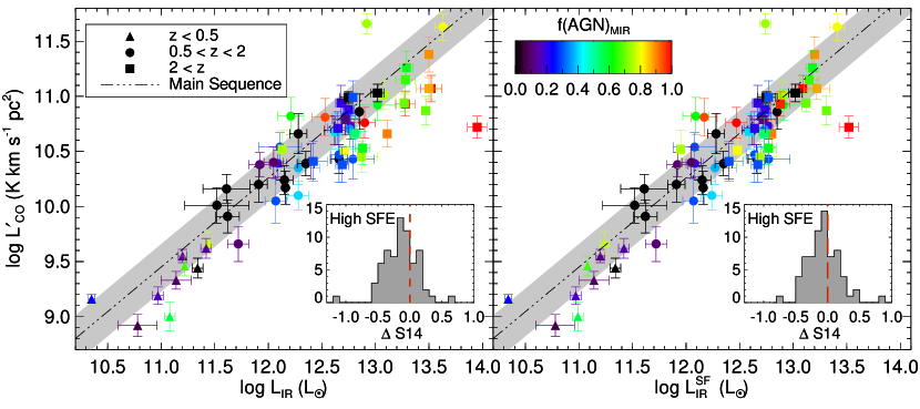
In the past, galaxies have conventionally been categorized in terms of two different modes of star formation: a main sequence-like “normal” mode (historically associated with local disk galaxies) and a starburst mode (historically associated with local U/LIRGs and frequently extended to high- SMGs). Normal star-forming galaxies have long gas depletion timescales of Myr (or for the depletion timescale’s inverse: high star formations efficiencies; SFEs), while starbursts are compact and have short gas depletion timescales. However, due to increased gas fractions, the relationship between compactness, main sequence, starburst, and SFE becomes increasingly murky with lookback time (e.g., Kartaltepe et al., 2012; Chang et al., 2018). For example, in a sample of IR selected galaxies, Kirkpatrick et al. (2014) demonstrate that the SFR/ criteria does not correlate with star formation efficiency. In addition, typical assumptions of bimodal CO-to- conversion factors may induce a separation between normal galaxies and starbursts (e.g. Daddi et al., 2010), and hinges on distinguishing reliably between a starburst galaxy and a normal galaxy, rather than assuming a smooth transition between the two regimes. In order to avoid the complicating choice of conversion factor, Carilli & Walter (2013) use a standard convention of comparing with as a proxy for SFE, where starbursting galaxies have higher star formation efficiencies manifested as an elevated for a given ( SFR) (see also Daddi et al., 2010; Genzel et al., 2010; Sargent et al., 2014). In Carilli & Walter (2013), radio AGN and QSOs had higher than main sequence selected galaxies.
In light of our recalculated homogeneous and values, and our quantitative/continuous approach to AGN emission, we revisit the relationship between and in Figure 5. We compare our sample to the - correlation for normal star formation in galaxies from Sargent et al. (2014). We should take care here to note that this relationship is not a main sequence of star formation in the way that the relationship between SFR and is (e.g. Noeske et al., 2007). Rather, it is the region of parameter space where most main sequence galaxies (the so-called normal population) tend to lie. But a galaxy in the grey regime in Figure 5 may not necessarily be a main sequence galaxy according to SFR/. Many of our galaxies lie off this norma relationship in the area of the graph (lower right) that would indicate a high SFE. This is not surprising since high- observations tend to be biased towards the brightest systems. As the relationship between and is meant to be a proxy for the relationship between molecular gas mass and SFR (i.e. an integrated form of the Schmidt-Kennicutt relation; Schmidt 1959; Kennicutt 1989), we should only be using the portion of due to star formation, . We therefore show vs. in the right panel of Figure 5. Using , almost every galaxy lies around the normal relation, which we quantify by calculating the difference in observed from the Sargent et al. (2014) prediction for normal star formation given a galaxy’s . Before the AGN correction, the geometric mean difference () is , where the negative indicates that sources are underluminous in CO, corresponding to a higher SFE. After the AGN correction, the mean difference is ; although it is small, this shift indicates how the presence of an AGN can bias interpretations of galaxy relationships if not properly accounted for.
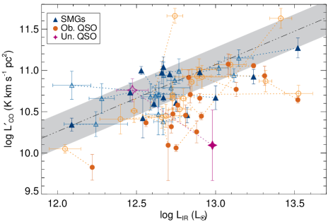
This result is noticeably differs from the recent work of Perna et al. (2018) which finds that obscured and unobscured QSOs from Carilli & Walter (2013) have higher SFEs. Of their sample, 30 submillimeter galaxies, 35 obscured quasars, and 6 unobscured quasars meet our selection criteria of being unlensed, at , and having a CO detection. Of these, only 15 SMGs, 18 obscured QSOs, and 1 unobscured QSO meet our criteria of having enough publicly available IR photometry to fully sample the SED. (All except 3 of these galaxies are drawn from the Carilli & Walter (2013) compilation.) Perna et al. (2018) determine using a spectral decomposition method that relies on the Chary & Elbaz (2001) and Dale & Helou (2002) templates derived from local galaxies. As we demonstrated in Kirkpatrick et al. (2012), IR luminous galaxies at have significantly different far-IR emission than the Chary & Elbaz (2001) library and require their own set of templates. In Figure 6, we show that the measurements from Perna et al. (2018) do indeed place QSOs in the region of high star formation efficiency. However, when calculating using high- templates that account for AGN emission and calculating using our new CO SLEDs, the same QSOs lie much closer to the main sequence. This result clearly illustrates that conclusions regarding how galaxies evolve critically depend on how the measurements are made.
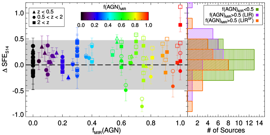
In Figure 7, we look for a correlation between black hole heating of the ISM and depressed star formation efficiency. We parameterize SFE as . We first use the Sargent et al. (2014) relation in Figure 5 to determine the SFE of normal galaxies. Then, we calculate the distance of our galaxies from this relation, . We plot as a function of in Figure 7. The shaded region represents a factor of 3 above and below the Sargent et al. (2014) SFE. There is no trend between and as confirmed by a Spearman’s rank test (, significance=0.85, which is not a statistically significant deviation from 0.0).
We split the sample at to measure whether low galaxies have a different distribution of than high galaxies. We plot the distributions in the right panel of Figure 7. A two-population Kolmogorov-Smirnov test cannot rule out the null hypothesis that of the two-subsamples are drawn from the same parent population. In other words, for our limited, heterogenous sample, there is no significant difference in the SFEs of high galaxies versus low galaxies. However, if we had not corrected for the AGN contribution when calculating SFE and , the two-population Kolmogorov-Smirnov test indicates that the distributions of for the SF-dominated and AGN-dominated galaxies significantly differ. We show the uncorrected s as the unfilled symbols in the left panel, and as the purple histogram in the right panel of Figure 7.
The star formation efficiency assumes that star formation is the dominant mode of consuming gas. Powerful AGN are also accreting gas, but at a much lower rate (e.g. Delvecchio et al., 2014). Massive outflows could expel gas, but estimates of this mass loss rate exist in only a handful of galaxies. In the local universe, an ionized mass loss rate of was measured in a Compton thick quasar (Revalski et al., 2018) and that outflow was solely attributed to its AGN (as opposed to a potential nuclear starburst); such outflow rates are not enough to drastically alter gas depletion timescales in AGN relative to normal SFGs. Gowardhan et al. (2018) find massive molecular outflows of hundreds of solar masses per year in two low redshift () ultra luminous infrared galaxies. In these galaxies, the molecular outflow is the dominant source depleting the gaseous ISM. However, the outflow correlates with both SFR and AGN luminosity, indicating that the AGN alone is not the dominant predictor of quenching-enabling feedback.
The fact that we do not observe lower SFE in AGN has three possible interpretations. First, our sample may be biased. Considering we have put together a heterogeneous, data-mined sample, we may be missing a key portion of galaxies that would exhibit enhanced or depleted SFE with increasing AGN energetics. However, for the sample that we have, we have taken care to measure properties and identify AGN in a homogeneous way. A large, blind IR survey followed with CO observations for all galaxies is the proper way to test gas depletion timescales in IR AGN.
A second potential reason for the lack of difference between the SFEs may be that IR AGN do not occur at special points in galaxies’ life cycles. (Kirkpatrick et al., 2012) showed that AGN are heating the central ISM relative to normal SFGs (indicated by rising warm dust emission from m; see also some discussion of AGN heating effects on CO in the following subsection). This heating may prevent star formation in the central 100 pc, and could be a significant contributor to quenching; verification of this effect requires future resolved observations of the ISM in the centers of IR AGN hosts. However, the lack of evidence for lower gas masses or shorter gas depletion timescales in our AGN suggests that AGN do not play a universal role in quenching star formation, even in massive galaxies (see also Xu et al., 2015). It leaves open the question of whether AGN are growing in lockstep with their galaxies, consuming the same fuel as the nascent stars (e.g., Kormendy & Ho, 2013, and references therein). If AGN are passively accreting in their hosts, rather than actively quenching, then why do only some galaxies have visible AGN? Either the triggering mechanisms of IR AGN do not seem to be universally responsible for enhanced star formation in dusty SFGs, as evidenced by our galaxies with high SFRs, short , but no AGN signatures, or the physics associated with AGN flickering make measuring any correlation hopeless.
Finally, we consider the possibility that the lack of difference between the SFEs may be rooted in the timescales of AGN activity. Theoretical models suggest that supermassive black holes go through growth spurts, causing a variable luminosity on 10,000 year timescales (Hickox et al., 2014) that would make correlations between AGN activity and SFR (or SFE) difficult to identify. In addition, the density of dust clouds in the torus cause it to cool quickly, from 1000 K to 100 K, in less than 10 years, (Ichikawa & Tazaki, 2017), making IR AGN unidentifiable when the supermassive black hole is not actively accreting. For such variable AGN, we may not expect to see a correlation between and SFE. The exact timescales traced by AGNs’ IR emission is relatively unconstrained, but it is likely extremely short ( Myr). IR-determined SFRs trace timescales of 100 Myr, so we may never see a correlation between the two phenomena, even if there is an underlying relationship. Finally, galaxies evolve over Gyr timescales. Given these differing ranges, looking for correlations between SFE and AGN activity may never reveal any information about the impact of AGN activity on its host galaxy.
Given the limitations potentially introduced by the timescales of AGN activity, we briefly consider whether progress might be made using future far-IR observations. As a back-of-the-envelope example, we assume the AGN heating can account for all dust emission at m in a galaxy with at m. If we assume that an AGN behaves as a compact emission source surrounded by a sphere of dust, then we can estimate the radius using . We use K, which gives pc. This is similar to the radius of the narrow line region, which extends 10-1000 pc (Groves et al., 2006; Hainline et al., 2013). At the extreme, if the AGN is heating the local diffuse cold neutral medium, beyond the ionized NLR, the main cooling is through the [CII] fine structure line. For thermal equilibrium, with a low density of , the cooling timescale is longer than 10,000 years. However, if the AGN’s influence is confined to the ionized narrow line region, then the cooling timescale will be much shorter (Groves et al., 2006; Hainline et al., 2016). Therefore, resolved 70 m observations (on scales of a kpc or less) may be a promising way to look for AGN emission over long timescales.
4.2. Average Gas Excitation Properties of AGN- and Starbust-dominated Galaxies
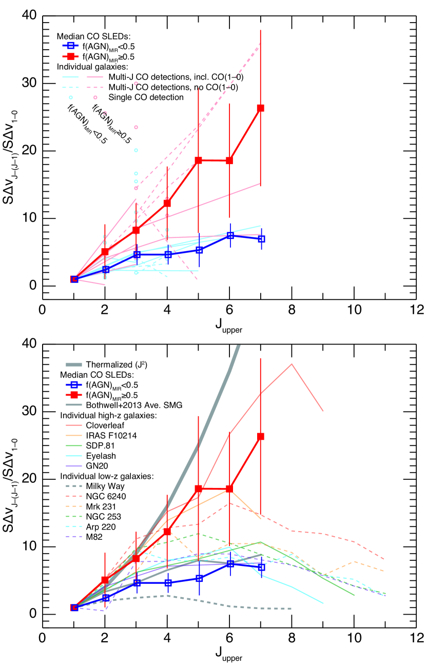
Using the methods described in Section 3.4, we also calculate the median CO SLEDs for galaxies with measured MIR AGN fractions (Table 2 and Figure 8). While the effects of AGN heating are likely continuous with , there are too few CO detection per source to look for fine-grained differences in the CO SLEDs as a function of . Therefore, as in the previous section, we divide the sources into two groups at in order to improve our statistics; for convenience, we refer to the sources below and above as SF-dominated and AGN-dominated respectively. In the bottom panel of Figure 8, we compare our new SLEDs to previous work (SLEDs for local ULIRGs are taken from Kamenetzky et al. 2016). Our median SF-dominated SLED closely resembles the average SMG SLED from Bothwell et al. (2013) and is also consistent with the SLEDs of local U/LIRGs such as Arp 220 and M82 (given our large uncertainties and the effects of small number statistics). Our median AGN-dominated SLED appears consistent with thermalized emission in the Rayleigh-Jeans limit (where flux ratios are equal to ). While thermalized emission is expected to arise in the dense molecular ISM of ULIRGs, SMGs, and AGN for low- lines (e.g., Weiß et al., 2007; Harris et al., 2010; Riechers et al., 2011a), it is generally not expected for the kinetic temperature to be sufficiently high to drive higher- emission to the asymptotic Rayleigh-Jeans limit. The consistency with thermalized emission for the high- lines in the AGN-dominated sample is likely due to the small number statistics that produce the considerable uncertainties. Significant amounts of high excitation emission is not uncommon for high- AGN, and our AGN-dominated SLED is consistent with that of the Cloverleaf galaxy and IRAS F10214+4724, which are both type 1 QSOs at . Local U/LIRGs with known AGN (i.e. NGC 6240, Mrk 231, and NGC 253) appear to have somewhat lower line ratios in their highest- transitions than we find in our median AGN-dominated SLED, but again they are consistent given our sample’s small numbers and large uncertainties. Given the uncertainties for our line ratios (Table 2), there is no significant difference between the CO excitation for the AGN-dominated galaxies () and the SF-dominated galaxies ().
| Transition | Ratio | Ratio | ||
|---|---|---|---|---|
| CO(1–0) | 8 | 8 | ||
| 16 | 5 | |||
| 15 | 18 | |||
| 7 | 5 | |||
| 2 | 3 | |||
| 1 | 1 | |||
| 1 | 4 | |||
However, there may be a systematic difference in the CO SLED for the two populations (Figure 8) even if individual line ratios are consistent within their uncertainty. In order to explore whether this systematic difference is significant, we compare the average emission line flux between the two populations for each CO line directly, thereby avoiding additional uncertainty from the CO(1–0) line when comparing the ratios between the two populations. We use a similar bootstrapping with replacement technique as described in Section 3.4 to determine the median line luminosities and their uncertainties for both samples, where line fluxes have been scaled linearly by the ratio of their individual IR luminosity to the median IR luminosity of the full sample (Figure 9). While there are still substantial uncertainties on the population ratios for each line, the observed trend with is statistically significant; performing a Spearman’s rank correlation test yields a chance of getting an observed correlation at least this strong with a null hypothesis of no correlation. However, this correlation is not robust. When removing either of the extrema from the correlation test (either the CO(1–0) population ratio or the CO(7–6) population ratio), the probability increases to , which is sufficiently large that we likely cannot rule out the null hypothesis of no correlation. In addition, if we Monte Carlo over the uncertainties (since the Spearman’s rank test does not factor those in), only of iterations yield of getting an observed correlation at least this strong. Therefore we must conclude that our data does not show a significant difference between the CO excitation of SF-dominated and AGN-dominated galaxies as defined by .
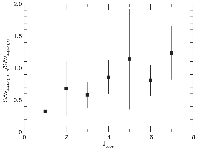
Ultimately, only two lines have detections in both the AGN-dominated and SF-dominated samples: the CO(1–0) line with eight detections below and above , and the CO(3–2) line with 15 and 18 detections below and above respectively (Table 2). We find that the ratio of CO(1–0) fluxes for the AGN-dominated to SF-dominated galaxies is , and the ratio for the CO(3–2) line is . At face value, these low-J ratios seem to indicate that for the same IR luminosity, galaxies with SF-dominated MIR fluxes have more gas than galaxies with AGN-dominated MIR fluxes. Such systematically lower gas masses in high- AGN might be expected if AGN play a role in quenching periods of rapid star formation or if AGN are temporally correlated with the transition between more bursty and more quiescent phases of galaxy evolution. However, this result would be at odds with the observed lack of difference in SFEs found in Section 4.1. Due to the small sample size, more data is needed before drawing strong conclusions.
This observed difference may be artificially produced by our method of linearly scaling using the ratio of the total (including both the contributions from star formation and any AGN) to some fiducial value.222Scaling by the do not change these result. If the correlation between and (the integrated Schmidt-Kennicutt relation) is super-linear (or sub-linear in the case of Fig. 5 where the axes are swapped), and of the AGN-dominated galaxies are dex brighter than the SF-dominated galaxies on average, then in the process of linearly scaling we effectively over-scale the gas emission of the AGN-dominated sources and correspondingly under-scale that for the SF-dominated sources. These scalings would then compound to produce the relatively lower ratios of AGN-to-SF gas masses. This effect of the scaling may come into play in the average SLEDs produced in Section 3.4, since AGN-dominated and SF-dominated galaxies are averaged together. If the total distributions differ systematically with galaxy class (or some other parameter of interest) that has systematically differing CO excitation, and the - is super-linear, then the net effect would be a bias towards the excitation characteristics of the lower luminosity population. If the index of the Schmidt-Kennicutt correlation becomes shallower for higher- CO gas tracers (e.g., Greve et al. 2014 and references therein; cf. Liu et al. 2015; Kamenetzky et al. 2016), then the applied scaling becomes systematically more appropriate for the higher- CO lines, and thus could also produce the observed correlation in Figure 9. In order to correct for such -dependent effects, either we would need new observations of a -matched sample with MIR-determined AGN fractions, or we would need to find some other parameter that linearly scales with gas mass to use when calculating the median CO luminosities. However, such scaling effects produced by the different populations’ distributions are removed by considering the higher- lines in ratio to the ground state (as for the CO SLED plots in Figure 8).
While high- CO emission from IR-bright AGN is well-documented (e.g., Downes et al., 1999; Bertoldi et al., 2003; Walter et al., 2003; Weiss et al., 2007; Gallerani et al., 2014; Tuan-Anh et al., 2017), we do not find conclusive evidence for systematically higher excitation CO SLEDs in this AGN-dominated sample. In spatially resolved studies of galaxies, it is well known that regions with different heating sources (and thus cloud physical conditions; i.e. temperatures and densities) will produce different CO line ratios—cold molecular clouds with moderate star formation rates in the peripheries of disk galaxies will produce sub-thermal emission at even the lowest- CO lines (e.g., for the outer disk of the Milky Way; Fixsen et al. 1999) while dense starbursts’ clouds or the central regions near AGN can produce nearly thermalized emission to much higher- (e.g., variations in the Antennae or near the central AGN of NGC 1068; Zhu et al. 2003; Spinoglio et al. 2012; Viti et al. 2014). Therefore, depending on the relative balance of these energy sources in each galaxy, we expect to measure different global line ratios (e.g., Harris et al., 2010; Narayanan & Krumholz, 2014). It follows that if the warm dust continuum emission from the AGN is dominating , and dust and molecular gas is comingled, then we might expect to see higher excitation is such systems’ CO SLEDs. Given the limitations of our current sample, we do not see evidence of this effect when comparing high- SFGs and IR AGN as defined by . Therefore, barring access to an -matched sample with MIR-determined AGN fractions (which will become possible in the era of JWST), increasing the number of multi-line CO detections (particularly at higher-) for archival Spitzer sources is likely the best way to improve statistics for the immediate future.
4.3. Evolving Gas-to-Dust Ratio
Due to the relatively modest time required for continuum observations as compared with gas emission lines submillimeter emission has recently been promoted as a gas mass tracer (e.g., Groves et al., 2015; Scoville et al., 2016). Calibrators for converting dust continuum emission into a gas mass rely on the assumption that the gas-to-dust mass ratio (GDR) is constant in solar metallicity galaxies out to . We can test this assumption, since we have independently measured dust and gas masses in a heterogeneous sample of galaxies out to , and we can look for changes in the GDR with increasing .
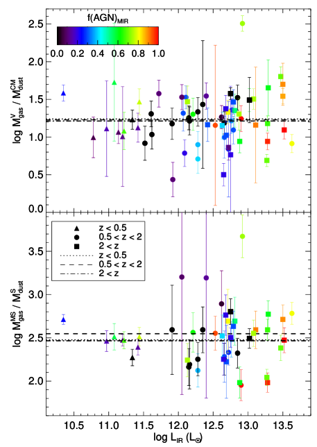
Figure 10 shows the GDR for our sample as a function of . In the top panel, we use a varying (Narayanan et al., 2012), and in the bottom panel, we use a constant for all galaxies, as described in Section 3.4.2. We determine the geometric mean of the GDR in three redshift bins and find it to be remarkably consistent; for a varying (constant) CO-to- conversion factor, the GDR is () for , () for , and () for . We find no trend in GDR with , and no difference in GDR between the sources above and below . The exact gas to dust ratio depends strongly on the assumed . It is difficult to know what the expected GDR at is, since it hinges so sensitively on and converting higher CO transitions to the ground state. In a sample of four solar metallicity galaxies at , Seko et al. (2016) use the CO(2-1) transition and and calculate GDRs in the range 220-1450, in agreement with our measurements. Saintonge et al. (2013) measured the GDR in 17 lensed galaxies at . They observe CO(3-2) and use a variable based on metallicity. They derive gas to dust ratios in the range of 100-700 and demonstrate that these values are 1.7 greater than local galaxies. For local galaxies, Leroy et al. (2011) presents a relation to derive GDR from metallicity. Based on the Leroy et al. (2011) relation, the expected average GDR of our galaxies is , closer to the value we derived following the Narayanan et al. (2012) method. The expected GDR, based on literature values for solar metallicity galaxies, is 100–200. The use of rather than would increase the GDR by a small amount (the most significant increase is for where the GDR increases to ).
The GDR calculted using the varying are very low. These low GDRs are due to the low gas masses inferred from the lower CO-to- conversion factors; these low conversion factors are either due to small radii used in calculating the CO surface brightness () or overestimated metallicities. Large (and thus low GDRs) could occur if dust and gas is not cospatial and the dust emission in high- SMGs is particularly compact (e.g., Hodge et al., 2016). If we assume that all galaxies have solar metallicity, then the average radius of the CO emission would need to be a factor of ten larger than the typical dust emission to produce GDR in all galaxies. Indeed, if we assume that all galaxies have solar metallicity, then there would be a consistent increase in GDR with redshift, so that by , GDR=34. Alternatively, if the low GDR is due to an overestimate of the metallicities, we would need to drop metallicities to in order to produce GDRs of . Such a drop in metallicity would imply a significant evolution in the relationship between and metallicity in massive galaxies as a function of redshift.
Assuming that any concerns with the CO-to- conversion factor are satisfied, our values of the GDR indicate that the varying assumptions used for calculating and likely require adjustment for galaxies beyond the local universe. Additional concerns about arise from estimating the gas phases at high redshift, particularly since more hydrogen may be in the molecular phase rather than the atomic phase compared with the local universe (Bertemes et al., 2018; Janowiecki et al., 2018). Regardless of method or assumptions, the GDR is consistent for all across the range of redshifts probed here. However, for individual objects, the ratios can vary significantly. Using the dust emission to estimate gas emission is likely only valid on average across large samples, rather than for individual objects.
5. Conclusions & Future Directions
We have compiled a heterogeneous sample of 67 galaxies from the literature that have CO line measurements and IR spectroscopy/photometry from . We have diagnosed the presence of an IR AGN using spectral decomposition or IR color selection based on techniques calibrated for galaxies at , and measured , , and consistently for all sources. Our findings are as follows:
-
1.
SFE is not strongly correlated with AGN emission. Strong AGN are observed to have both high and low star formation efficiencies, indicating that the presence of an AGN itself does not indicate a galaxy is beginning to quench. Any expected correlation may necessarily be murky due to AGN luminosity flickering on much shorter timescales than galaxy evolution.
-
2.
It is important to fully sample the IR SED, use appropriate templates, and take AGN heating effects into account when calculating . If this is not done, derived SFRs will be too high and SFE will wrongly appear to be enhanced in IR AGN.
-
3.
Gas-to-dust ratios do not appear to evolve with redshift for this heterogeneous sample, although the scatter is large. We find consistent gas-to-dust ratios regardless of redshift, luminosity, or AGN strength. However, for individual objects, the exact gas to dust ratio can vary significantly.
-
4.
We do not find a statistically significant difference in the CO excitation for individual line ratios for galaxies above and below . While it appears that the median CO SLED of sources with is at systematically higher excitation than median CO SLED of galaxies with for all rotational transitions, this result is not robust statistically.
Many of our conclusions about the molecular gas content and the effects of AGN heating is limited by small number statistics and the lack of matched luminosity samples. A systematic CO SLED survey of galaxies with known IR AGN content (i.e. measured ) is critical for disentangling evidence of AGN feedback affecting star-forming molecular gas via the gas physical conditions. Since the problem of high SFRs that require some limiting mechanism to prevent the over-production of massive galaxies today is particularly acute among dusty SFGs, studies of AGN feedback are more likely to be successful when focused on high- IR-bright galaxies such as SMGs. Since comparing average gas properties requires scaling out the dominant effect of brighter/more-massive galaxies being brighter across the electromagnetic spectrum (to first order), accurate normalization is similarly critical. Firmer conclusions could be reached with either (a) more observations of the CO(1–0) line to normalize the excitation, (b) more observations of the CO lines where the number of detections for samples are lowest, or (c) developing matched IR luminosity samples among IR AGN and SFGs. Until we have the mid-IR spectroscopic/photometric capabilities of JWST that enable the selection of matched samples of high- galaxies, we are restricted to analyzing galaxies with archival Sptizer data.
AK thanks Sukanya Chakrabarti and Desika Narayanan for helpful conversations. AK gratefully acknowledges support from the YCAA Prize Postdoctoral Fellowship.
| Name | RA | Dec | z | aaThese sources had Spitzer IRS spectroscopy which was decomposed to measure the mid-IR AGN fraction. | ||
|---|---|---|---|---|---|---|
| 5MUSES-179 | 16:08:03.71 | +54:53:02.0 | 0.053 | 0.24aaThese sources had Spitzer IRS spectroscopy which was decomposed to measure the mid-IR AGN fraction. | ||
| 5MUSES-169 | 16:04:08.30 | +54:58:13.1 | 0.064 | 0.06aaThese sources had Spitzer IRS spectroscopy which was decomposed to measure the mid-IR AGN fraction. | ||
| 5MUSES-105 | 10:44:32.94 | +56:40:41.6 | 0.068 | 0.16aaThese sources had Spitzer IRS spectroscopy which was decomposed to measure the mid-IR AGN fraction. | ||
| 5MUSES-171 | 16:04:40.64 | +55:34:09.3 | 0.078 | 0.08aaThese sources had Spitzer IRS spectroscopy which was decomposed to measure the mid-IR AGN fraction. | ||
| 5MUSES-229 | 16:18:19.31 | +54:18:59.1 | 0.082 | 0.12aaThese sources had Spitzer IRS spectroscopy which was decomposed to measure the mid-IR AGN fraction. | ||
| 5MUSES-132 | 10:52:06.56 | +58:09:47.1 | 0.117 | 0.00aaThese sources had Spitzer IRS spectroscopy which was decomposed to measure the mid-IR AGN fraction. | ||
| 5MUSES-227 | 16:17:59.22 | +54:15:01.3 | 0.134 | 0.57aaThese sources had Spitzer IRS spectroscopy which was decomposed to measure the mid-IR AGN fraction. | ||
| 5MUSES-141 | 10:57:05.43 | +58:04:37.4 | 0.140 | 0.67aaThese sources had Spitzer IRS spectroscopy which was decomposed to measure the mid-IR AGN fraction. | ||
| 5MUSES-136 | 10:54:21.65 | +58:23:44.7 | 0.204 | 0.77aaThese sources had Spitzer IRS spectroscopy which was decomposed to measure the mid-IR AGN fraction. | ||
| 5MUSES-216 | 16:15:51.45 | +54:15:36.0 | 0.215 | 0.14aaThese sources had Spitzer IRS spectroscopy which was decomposed to measure the mid-IR AGN fraction. | ||
| PEPJ123646+621141 | 12:36:46.18 | +62:11:42.0 | 1.016 | 0.00 | ||
| GN70.38aaThese sources had Spitzer IRS spectroscopy which was decomposed to measure the mid-IR AGN fraction. | 12:36:33.68 | +62:10:05.9 | 1.016 | 0.00aaThese sources had Spitzer IRS spectroscopy which was decomposed to measure the mid-IR AGN fraction. | ||
| EGS13035123 | 14:20:05.40 | +53:01:15.4 | 1.070 | 0.20 | ||
| PEPJ123759+621732 | 12:37:59.47 | +62:17:32.9 | 1.084 | 0.00 | ||
| GN70.8 | 12:36:20.94 | +62:07:14.2 | 1.148 | 0.00aaThese sources had Spitzer IRS spectroscopy which was decomposed to measure the mid-IR AGN fraction. | ||
| PEPJ123750+621600 | 12:37:50.89 | +62:16:00.7 | 1.170 | 0.00 | ||
| SMMJ163658+405728 | 16:36:58.78 | +40:57:27.6 | 1.193 | 0.38aaThese sources had Spitzer IRS spectroscopy which was decomposed to measure the mid-IR AGN fraction. | ||
| EGS13003805 | 14:19:40.08 | +52:49:38.6 | 1.200 | 0.30 | ||
| J123634.53+621241.3 | 12:36:34.57 | +62:12:41.0 | 1.223 | 0.04aaThese sources had Spitzer IRS spectroscopy which was decomposed to measure the mid-IR AGN fraction. | ||
| GN70.104 | 12:37:02.74 | +63:14:01.5 | 1.246 | 0.00aaThese sources had Spitzer IRS spectroscopy which was decomposed to measure the mid-IR AGN fraction. | ||
| PEPJ123712+621753 | 12:37:12.15 | +62:17:54.0 | 1.249 | 0.10 | ||
| SMMJ030227+000653 | 03:02:27.66 | +00:06:53.0 | 1.406 | 0.00aaThese sources had Spitzer IRS spectroscopy which was decomposed to measure the mid-IR AGN fraction. | ||
| EGS13004291 | 14:19:14.96 | +52:49:30.1 | 1.410 | 0.20 | ||
| no.226 | 03:32:15.99 | -27:48:59.4 | 1.413 | 0.30 | ||
| RGJ123645.88+620754.2 | 12:36:45.88 | +62:07:54.2 | 1.434 | 0.13aaThese sources had Spitzer IRS spectroscopy which was decomposed to measure the mid-IR AGN fraction. | ||
| 3C298 | 14:19:08.18 | +06:28:34.8 | 1.438 | 0.80 | ||
| HR10 | 16:45:02.26 | +46:26:26.5 | 1.440 | 0.27aaThese sources had Spitzer IRS spectroscopy which was decomposed to measure the mid-IR AGN fraction. | ||
| BzK-4171 | 12:36:26.52 | +62:08:35.4 | 1.465 | 0.09aaThese sources had Spitzer IRS spectroscopy which was decomposed to measure the mid-IR AGN fraction. | ||
| 51613 | 10:02:43.36 | +01:34:20.9 | 1.517 | 0.10 | ||
| BzK-21000 | 12:37:10.60 | +62:22:34.6 | 1.523 | 0.00aaThese sources had Spitzer IRS spectroscopy which was decomposed to measure the mid-IR AGN fraction. | ||
| 51858 | 10:02:40.43 | +01:34:13.1 | 1.556 | 0.40 | ||
| MIPS8342 | 17:14:11.55 | +60:11:09.3 | 1.562 | 0.74a,ba,bfootnotemark: | ||
| 3C318 | 05:20:05.49 | +20:16:05.7 | 1.577 | 1.00aaThese sources had Spitzer IRS spectroscopy which was decomposed to measure the mid-IR AGN fraction. | ||
| SMMJ105151+572636 | 10:51:51.77 | +57:26:35.3 | 1.597 | 0.30aaThese sources had Spitzer IRS spectroscopy which was decomposed to measure the mid-IR AGN fraction. | ||
| COSB011 | 10:00:38.02 | +02:08:22.9 | 1.827 | 0.60 | ||
| SMMJ123555+620901 | 12:35:54.85 | +62:08:54.7 | 1.864 | 0.63a,ba,bfootnotemark: | ||
| SMMJ123632+620800 | 12:36:33.04 | +62:08:05.1 | 1.994 | 0.95a,ba,bfootnotemark: | ||
| SMMJ123712+621322 | 12:37:12.12 | +62:13:22.2 | 1.996 | 0.00aaThese sources had Spitzer IRS spectroscopy which was decomposed to measure the mid-IR AGN fraction. | ||
| SMMJ123618.33+621550.5 | 12:36:18.47 | +62:15:51.0 | 1.996 | 0.36aaThese sources had Spitzer IRS spectroscopy which was decomposed to measure the mid-IR AGN fraction. | ||
| SMMJ123711+621325 | 12:37:11.19 | +62:13:31.2 | 1.996 | 0.00aaThese sources had Spitzer IRS spectroscopy which was decomposed to measure the mid-IR AGN fraction. | ||
| RG J123711 | 12:37:11.34 | +62:32:31.0 | 1.996 | 0.30 | ||
| MIPS16080 | 17:18:44.77 | +60:01:15.9 | 2.006 | 0.81a,ba,bfootnotemark: | ||
| SMMJ021738-050339 | 02:17:38.68 | -05:03:39.3 | 2.037 | 0.20 | ||
| RG J123644.13+621450.7 | 12:36:44.13 | +62:14:50.7 | 2.095 | 0.75aaThese sources had Spitzer IRS spectroscopy which was decomposed to measure the mid-IR AGN fraction. | ||
| HS1002+4400 | 10:05:17.43 | +43:46:09.3 | 2.102 | 1.00aaThese sources had Spitzer IRS spectroscopy which was decomposed to measure the mid-IR AGN fraction. | ||
| MIPS15949 | 17:21:09.22 | +60:15:01.3 | 2.119 | 0.91a,ba,bfootnotemark: | ||
| MIPS16144 | 17:24:22.09 | +59:31:50.8 | 2.128 | 0.11aaThese sources had Spitzer IRS spectroscopy which was decomposed to measure the mid-IR AGN fraction. | ||
| MIPS429 | 17:16:11.83 | +59:12:13.2 | 2.201 | 0.54aaThese sources had Spitzer IRS spectroscopy which was decomposed to measure the mid-IR AGN fraction. | ||
| SMMJ123549+6215 | 12:35:49.43 | +62:15:36.7 | 2.202 | 0.20 | ||
| RXJ124913.86-055906.2 | 12:49:13.85 | -05:59:19.4 | 2.247 | 1.00aaThese sources had Spitzer IRS spectroscopy which was decomposed to measure the mid-IR AGN fraction. | ||
| SMMJ021725-045934 | 02:17:25.16 | -04:59:34.9 | 2.292 | 0.40 | ||
| MIPS16059 | 17:24:28.45 | +60:15:33.0 | 2.326 | 0.75a,ba,bfootnotemark: | ||
| SMMJ16371+4053 | 16:37:06.50 | +40:53:14.0 | 2.377 | 0.60bbWe identified these sources as IR AGN, but they are classified as SFGs in Carilli & Walter (2013). | ||
| SMMJ163650+405734 | 16:36:50.41 | +40:57:34.4 | 2.385 | 0.75a,ba,bfootnotemark: | ||
| SMMJ105227+572512 | 10:52:27.10 | +57:25:16.0 | 2.440 | 0.30 | ||
| SMMJ16358+4105 | 16:36:58.20 | +41:05:24.0 | 2.450 | 0.00 | ||
| SMMJ123707+6214 | 12:37:07.28 | +62:14:08.6 | 2.488 | 0.00aaThese sources had Spitzer IRS spectroscopy which was decomposed to measure the mid-IR AGN fraction. | ||
| SMMJ123606+621047 | 12:36:06.85 | +62:10:21.4 | 2.505 | 0.30 | ||
| SMMJ221804+002154 | 22:18:04.42 | +00:21:54.4 | 2.517 | 0.20 | ||
| SMMJ021738-050528 | 02:17:38.88 | -05:05:28.2 | 2.541 | 0.30 | ||
| VCV J1409+5628 | 14:09:55.50 | +56:28:27.0 | 2.583 | 0.98aaThese sources had Spitzer IRS spectroscopy which was decomposed to measure the mid-IR AGN fraction. | ||
| AMS12 | 17:18:22.65 | +59:01:54.3 | 2.766 | 0.70 | ||
| SMMJ04135+10277 | 04:13:27.28 | +10:27:40.4 | 2.846 | 0.70bbWe identified these sources as IR AGN, but they are classified as SFGs in Carilli & Walter (2013). | ||
| B3 J2330+3927 | 23:30:24.84 | +39:37:12.2 | 3.094 | 0.90 | ||
| 6C1909+722 | 19:08:23.70 | +72:20:11.6 | 3.532 | 0.88aaThese sources had Spitzer IRS spectroscopy which was decomposed to measure the mid-IR AGN fraction. | ||
| 4C41.17 | 06:50:52.10 | +41:30:30.5 | 3.796 | 0.60 | ||
| GN20 | 12:37:11.86 | +62:22:12.6 | 4.055 | 0.66aaThese sources had Spitzer IRS spectroscopy which was decomposed to measure the mid-IR AGN fraction. |
| Name | aaVariable calculated from Narayanan et al. (2012). | (kpc)bbISM radius, , and are the parameters derived by fitting a radiative transfer model to far-IR photometry using the method of Chakrabarti & McKee (2008). | bbISM radius, , and are the parameters derived by fitting a radiative transfer model to far-IR photometry using the method of Chakrabarti & McKee (2008). | cc is calculated using the formalism of Scoville et al. (2016). | dd is calculated using the variable in Column 2. Errors are the same as for in Table 3. | ee is calculated using a single for every galaxy. Errors are the same as for in Table 3. |
|---|---|---|---|---|---|---|
| 5MUSES-179 | 0.45 | 0.11 | 8.81 | 9.82 | ||
| 5MUSES-169 | 0.42 | 0.10 | 8.55 | 9.58 | ||
| 5MUSES-105 | 0.26 | 0.06 | 8.60 | 9.85 | ||
| 5MUSES-171 | 0.39 | 0.19 | 8.92 | 9.99 | ||
| 5MUSES-229 | 0.21 | 0.09 | 8.87 | 10.21 | ||
| 5MUSES-132 | 0.41 | 0.22 | 9.05 | 10.10 | ||
| 5MUSES-227 | 0.24 | 0.02 | 8.38 | 9.66 | ||
| 5MUSES-141 | 0.30 | 0.14 | 8.93 | 10.12 | ||
| 5MUSES-136 | 0.29 | 0.15 | 9.14 | 10.33 | ||
| 5MUSES-216 | 0.30 | 0.19 | 9.09 | 10.28 | ||
| PEPJ123646+621141 | 0.28 | 0.34 | 9.36 | 10.57 | ||
| GN70.38 | 0.22 | 0.35 | 9.56 | 10.86 | ||
| EGS13035123 | 0.22 | 0.67 | 9.73 | 11.05 | ||
| PEPJ123759+621732 | 0.25 | 0.36 | 9.41 | 10.67 | ||
| GN70.8 | 0.24 | 0.36 | 9.55 | 10.83 | ||
| PEPJ123750+621600 | 0.24 | 0.33 | 9.55 | 10.82 | ||
| SMMJ163658+405728 | 0.25 | 0.74 | 9.75 | 11.01 | ||
| EGS13003805 | 0.21 | 0.43 | 9.86 | 11.20 | ||
| J123634.53+621241.3 | 0.20 | 0.67 | 9.98 | 11.35 | ||
| GN70.104 | 0.25 | 0.42 | 9.63 | 10.90 | ||
| PEPJ123712+621753 | 0.35 | 0.19 | 9.21 | 10.32 | ||
| SMMJ030227+000653 | 0.24 | 0.64 | 9.82 | 11.09 | ||
| EGS13004291 | 0.18 | 0.57 | 9.99 | 11.39 | ||
| no.226 | 0.24 | 0.26 | 9.44 | 10.71 | ||
| RG J123645.88+620754.2 | 0.24 | 0.42 | 9.78 | 11.07 | ||
| 3C298 | 0.23 | 8.22 | 10.98 | 12.29 | ||
| HR10 | 0.10 | 0.31 | 9.80 | 11.48 | ||
| BzK-4171 | 0.21 | 0.34 | 9.73 | 11.06 | ||
| 51613 | 0.20 | 0.75 | 9.68 | 11.04 | ||
| BzK-21000 | 0.10 | 0.08 | 9.38 | 11.05 | ||
| 51858 | 0.26 | 0.55 | 9.51 | 10.76 | ||
| MIPS8342 | 0.10 | 0.44 | 10.67 | 12.32 | ||
| 3C318 | 0.17 | 0.60 | 9.99 | 11.42 | ||
| SMMJ105151+572636 | 0.20 | 0.57 | 9.78 | 11.13 | ||
| COSB011 | 0.18 | 0.75 | 10.18 | 11.58 | ||
| SMMJ123555+620901 | 0.15 | 0.51 | 10.00 | 11.48 | ||
| SMMJ123632+620800 | 0.08 | 0.15 | 9.70 | 11.47 | ||
| SMMJ123712+621322 | 0.22 | 0.74 | 10.00 | 11.32 | ||
| SMMJ123618.33+621550.5 | 0.23 | 0.94 | 10.06 | 11.36 | ||
| SMMJ123711+621325 | 0.20 | 0.78 | 10.16 | 11.52 | ||
| RG J123711 | 0.30 | 1.07 | 9.91 | 11.09 | ||
| MIPS16080 | 0.22 | 0.56 | 9.86 | 11.17 | ||
| SMMJ021738-050339 | 0.17 | 0.74 | 10.17 | 11.60 | ||
| RGJ123644.13+621450.7 | 0.19 | 0.35 | 9.79 | 11.18 | ||
| HS1002+4400 | 0.38 | 5.99 | 10.64 | 11.73 | ||
| MIPS15949 | 0.09 | 0.16 | 9.63 | 11.32 | ||
| MIPS16144 | 0.19 | 1.11 | 10.07 | 11.45 | ||
| MIPS429 | 0.15 | 0.35 | 9.84 | 11.32 | ||
| SMMJ123549+6215 | 0.08 | 0.28 | 9.79 | 11.54 | ||
| RXJ124913.86-055906.2 | 0.41 | 5.99 | 10.34 | 11.38 | ||
| SMMJ021725-045934 | 0.20 | 0.72 | 9.97 | 11.34 | ||
| MIPS16059 | 0.18 | 0.33 | 9.70 | 11.11 | ||
| SMMJ16371+4053 | 0.37 | 2.24 | 10.10 | 11.19 | ||
| SMMJ163650+405734 | 0.20 | 1.04 | 10.30 | 11.67 | ||
| SMMJ105227+572512 | 0.25 | 0.72 | 9.78 | 11.04 | ||
| SMMJ16358+4105 | 0.10 | 0.28 | 10.02 | 11.69 | ||
| SMMJ123707+6214 | 0.17 | 0.69 | 10.22 | 11.65 | ||
| SMMJ123606+621047 | 0.20 | 0.43 | 9.71 | 11.07 | ||
| SMMJ221804+002154 | 0.42 | 5.99 | 10.33 | 11.37 | ||
| SMMJ021738-050528 | 0.18 | 0.83 | 10.24 | 11.65 | ||
| VCV J1409+5628 | 0.48 | 8.35 | 10.61 | 11.59 | ||
| AMS12 | 0.73 | 7.68 | 10.73 | 11.53 | ||
| SMMJ04135+10277 | 0.50 | 11.57 | 10.64 | 11.60 | ||
| B3 J2330+3927 | 0.08 | 0.33 | 10.29 | 12.04 | ||
| 6C1909+722 | 0.25 | 1.76 | 10.46 | 11.73 | ||
| 4C41.17 | 0.08 | 0.25 | 10.15 | 11.92 | ||
| GN20 | 0.37 | 6.39 | 10.72 | 11.81 |
References
- Ao et al. (2008) Ao, Y., Weiß, A., Downes, D., et al. 2008, A&A, 491, 747
- Aravena et al. (2014) Aravena, M., Hodge, J. A., Wagg, J., et al. 2014, MNRAS, 442, 558
- Bertemes et al. (2018) Bertemes, C., Wuyts, S., Lutz, D., et al. 2018, MNRAS, 478, 1442
- Bertoldi et al. (2003) Bertoldi, F., Cox, P., Neri, R., et al. 2003, A&A, 409, L47
- Blain (1999) Blain, A. W. 1999, MNRAS, 304, 669
- Bolatto et al. (2013) Bolatto, A. D., Wolfire, M., & Leroy, A. K. 2013, ARA&A, 51, 207
- Bothwell et al. (2013) Bothwell, M. S., Smail, I., Chapman, S. C., et al. 2013, MNRAS, 429, 3047
- Bouché et al. (2010) Bouché, N., Dekel, A., Genzel, R., et al. 2010, ApJ, 718, 1001
- Brinchmann et al. (2004) Brinchmann, J., Charlot, S., White, S. D. M., et al. 2004, MNRAS, 351, 1151
- Caplar et al. (2018) Caplar, N., Lilly, S. J., & Trakhtenbrot, B. 2018, ApJ, 867, 148
- Carilli & Walter (2013) Carilli, C. L., & Walter, F. 2013, ARA&A, 51, 105
- Casey et al. (2014) Casey, C. M., Narayanan, D., & Cooray, A. 2014, Phys. Rep., 541, 45
- Chakrabarti & McKee (2005) Chakrabarti, S., & McKee, C. F. 2005, ApJ, 631, 792
- Chakrabarti & McKee (2008) —. 2008, ApJ, 683, 693
- Chang et al. (2018) Chang, Y.-Y., Ferraro, N., Wang, W.-H., et al. 2018, ApJ, 865, 103
- Chary & Elbaz (2001) Chary, R., & Elbaz, D. 2001, ApJ, 556, 562
- Cicone et al. (2014) Cicone, C., Maiolino, R., Sturm, E., et al. 2014, A&A, 562, A21
- Croton et al. (2006) Croton, D. J., Springel, V., White, S. D. M., et al. 2006, MNRAS, 365, 11
- da Cunha et al. (2013) da Cunha, E., Groves, B., Walter, F., et al. 2013, ApJ, 766, 13
- Daddi et al. (2007) Daddi, E., Dickinson, M., Morrison, G., et al. 2007, ApJ, 670, 156
- Daddi et al. (2010) Daddi, E., Elbaz, D., Walter, F., et al. 2010, ApJ, 714, L118
- Dale & Helou (2002) Dale, D. A., & Helou, G. 2002, ApJ, 576, 159
- Davé et al. (2011) Davé, R., Oppenheimer, B. D., & Finlator, K. 2011, MNRAS, 415, 11
- Delvecchio et al. (2014) Delvecchio, I., Gruppioni, C., Pozzi, F., et al. 2014, MNRAS, 439, 2736
- Downes et al. (1999) Downes, D., Neri, R., Wiklind, T., Wilner, D. J., & Shaver, P. A. 1999, ApJ, 513, L1
- Draine (2003) Draine, B. T. 2003, ARA&A, 41, 241
- Draine & Li (2007) Draine, B. T., & Li, A. 2007, ApJ, 657, 810
- Elbaz et al. (2007) Elbaz, D., Daddi, E., Le Borgne, D., et al. 2007, A&A, 468, 33
- Elvis et al. (1994) Elvis, M., Wilkes, B. J., McDowell, J. C., et al. 1994, ApJS, 95, 1
- Ferrarese & Merritt (2000) Ferrarese, L., & Merritt, D. 2000, ApJ, 539, L9
- Feruglio et al. (2010) Feruglio, C., Maiolino, R., Piconcelli, E., et al. 2010, A&A, 518, L155
- Fiore et al. (2017) Fiore, F., Feruglio, C., Shankar, F., et al. 2017, A&A, 601, A143
- Fixsen et al. (1999) Fixsen, D. J., Bennett, C. L., & Mather, J. C. 1999, ApJ, 526, 207
- Frayer et al. (2018) Frayer, D. T., Maddalena, R. J., Ivison, R. J., et al. 2018, ArXiv e-prints, arXiv:1805.07212
- French et al. (2015) French, K. D., Yang, Y., Zabludoff, A., et al. 2015, ApJ, 801, 1
- French et al. (2018) French, K. D., Zabludoff, A. I., Yoon, I., et al. 2018, ApJ, 861, 123
- Gabor et al. (2011) Gabor, J. M., Davé, R., Oppenheimer, B. D., & Finlator, K. 2011, MNRAS, 417, 2676
- Gallerani et al. (2014) Gallerani, S., Ferrara, A., Neri, R., & Maiolino, R. 2014, MNRAS, 445, 2848
- Gebhardt et al. (2000) Gebhardt, K., Bender, R., Bower, G., et al. 2000, ApJ, 539, L13
- Genzel et al. (2010) Genzel, R., Tacconi, L. J., Gracia-Carpio, J., et al. 2010, MNRAS, 407, 2091
- Glikman et al. (2012) Glikman, E., Urrutia, T., Lacy, M., et al. 2012, ApJ, 757, 51
- Goulding et al. (2018) Goulding, A. D., Greene, J. E., Bezanson, R., et al. 2018, PASJ, 70, S37
- Gowardhan et al. (2018) Gowardhan, A., Spoon, H., Riechers, D. A., et al. 2018, ApJ, 859, 35
- Greve et al. (2014) Greve, T. R., Leonidaki, I., Xilouris, E. M., et al. 2014, ApJ, 794, 142
- Groves et al. (2006) Groves, B., Dopita, M., & Sutherland, R. 2006, A&A, 458, 405
- Groves et al. (2015) Groves, B. A., Schinnerer, E., Leroy, A., et al. 2015, ApJ, 799, 96
- Hailey-Dunsheath et al. (2012) Hailey-Dunsheath, S., Sturm, E., Fischer, J., et al. 2012, ApJ, 755, 57
- Hainline et al. (2013) Hainline, K. N., Hickox, R., Greene, J. E., Myers, A. D., & Zakamska, N. L. 2013, ApJ, 774, 145
- Hainline et al. (2016) Hainline, K. N., Hickox, R. C., Chen, C.-T., et al. 2016, ApJ, 823, 42
- Harris et al. (2010) Harris, A. I., Baker, A. J., Zonak, S. G., et al. 2010, ApJ, 723, 1130
- Harrison et al. (2012) Harrison, C. M., Alexander, D. M., Mullaney, J. R., et al. 2012, ApJ, 760, L15
- Herrera-Camus et al. (2019) Herrera-Camus, R., Tacconi, L., Genzel, R., et al. 2019, ApJ, 871, 37
- Hezaveh et al. (2012) Hezaveh, Y. D., Marrone, D. P., & Holder, G. P. 2012, ApJ, 761, 20
- Hickox et al. (2014) Hickox, R. C., Mullaney, J. R., Alexander, D. M., et al. 2014, ApJ, 782, 9
- Hodge et al. (2015) Hodge, J. A., Riechers, D., Decarli, R., et al. 2015, ApJ, 798, L18
- Hodge et al. (2016) Hodge, J. A., Swinbank, A. M., Simpson, J. M., et al. 2016, ApJ, 833, 103
- Hodge et al. (2018) Hodge, J. A., Smail, I., Walter, F., et al. 2018, ArXiv e-prints, arXiv:1810.12307
- Hopkins et al. (2006) Hopkins, P. F., Somerville, R. S., Hernquist, L., et al. 2006, ApJ, 652, 864
- Hunt et al. (2018) Hunt, Q., Bezanson, R., Greene, J. E., et al. 2018, ApJ, 860, L18
- Ichikawa & Tazaki (2017) Ichikawa, K., & Tazaki, R. 2017, ApJ, 844, 21
- Ishibashi & Fabian (2012) Ishibashi, W., & Fabian, A. C. 2012, MNRAS, 427, 2998
- Janowiecki et al. (2018) Janowiecki, S., Cortese, L., Catinella, B., & Goodwin, A. J. 2018, MNRAS, 476, 1390
- Kamenetzky et al. (2016) Kamenetzky, J., Rangwala, N., Glenn, J., Maloney, P. R., & Conley, A. 2016, ApJ, 829, 93
- Kartaltepe et al. (2012) Kartaltepe, J. S., Dickinson, M., Alexander, D. M., et al. 2012, ApJ, 757, 23
- Kennicutt (1989) Kennicutt, Jr., R. C. 1989, ApJ, 344, 685
- Kim et al. (2013) Kim, C.-G., Ostriker, E. C., & Kim, W.-T. 2013, ApJ, 776, 1
- Kirkpatrick et al. (2015) Kirkpatrick, A., Pope, A., Sajina, A., et al. 2015, ApJ, 814, 9
- Kirkpatrick et al. (2012) Kirkpatrick, A., Pope, A., Alexander, D. M., et al. 2012, ApJ, 759, 139
- Kirkpatrick et al. (2014) Kirkpatrick, A., Pope, A., Aretxaga, I., et al. 2014, ApJ, 796, 135
- Kirkpatrick et al. (2017) Kirkpatrick, A., Alberts, S., Pope, A., et al. 2017, ApJ, 849, 111
- Kocevski et al. (2017) Kocevski, D. D., Barro, G., Faber, S. M., et al. 2017, ApJ, 846, 112
- Kormendy & Ho (2013) Kormendy, J., & Ho, L. C. 2013, ARA&A, 51, 511
- Leroy et al. (2011) Leroy, A. K., Bolatto, A., Gordon, K., et al. 2011, ApJ, 737, 12
- Lilly et al. (2013) Lilly, S. J., Carollo, C. M., Pipino, A., Renzini, A., & Peng, Y. 2013, ApJ, 772, 119
- Liu et al. (2015) Liu, D., Gao, Y., Isaak, K., et al. 2015, ApJ, 810, L14
- Mahoro et al. (2017) Mahoro, A., Pović, M., & Nkundabakura, P. 2017, MNRAS, 471, 3226
- Misselt et al. (2001) Misselt, K. A., Gordon, K. D., Clayton, G. C., & Wolff, M. J. 2001, ApJ, 551, 277
- Mullaney et al. (2011) Mullaney, J. R., Alexander, D. M., Goulding, A. D., & Hickox, R. C. 2011, MNRAS, 414, 1082
- Murphy et al. (2011) Murphy, E. J., Condon, J. J., Schinnerer, E., et al. 2011, ApJ, 737, 67
- Narayanan & Krumholz (2014) Narayanan, D., & Krumholz, M. R. 2014, MNRAS, 442, 1411
- Narayanan et al. (2012) Narayanan, D., Krumholz, M. R., Ostriker, E. C., & Hernquist, L. 2012, MNRAS, 421, 3127
- Narayanan et al. (2015) Narayanan, D., Turk, M., Feldmann, R., et al. 2015, Nature, 525, 496
- Noeske et al. (2007) Noeske, K. G., Weiner, B. J., Faber, S. M., et al. 2007, ApJ, 660, L43
- Page et al. (2012) Page, M. J., Symeonidis, M., Vieira, J. D., et al. 2012, Nature, 485, 213
- Perna et al. (2018) Perna, M., Sargent, M. T., Brusa, M., et al. 2018, A&A, 619, A90
- Pontzen et al. (2017) Pontzen, A., Tremmel, M., Roth, N., et al. 2017, MNRAS, 465, 547
- Pope et al. (2008) Pope, A., Chary, R.-R., Alexander, D. M., et al. 2008, ApJ, 675, 1171
- Pope et al. (2013) Pope, A., Wagg, J., Frayer, D., et al. 2013, ApJ, 772, 92
- Rémy-Ruyer et al. (2015) Rémy-Ruyer, A., Madden, S. C., Galliano, F., et al. 2015, A&A, 582, A121
- Revalski et al. (2018) Revalski, M., Dashtamirova, D., Crenshaw, D. M., et al. 2018, ApJ, 867, 88
- Ricci et al. (2017) Ricci, C., Assef, R. J., Stern, D., et al. 2017, ApJ, 835, 105
- Riechers et al. (2011a) Riechers, D. A., Carilli, C. L., Maddalena, R. J., et al. 2011a, ApJ, 739, L32
- Riechers et al. (2011b) Riechers, D. A., Carilli, L. C., Walter, F., et al. 2011b, ApJ, 733, L11
- Rosenberg et al. (2015) Rosenberg, M. J. F., van der Werf, P. P., Aalto, S., et al. 2015, ApJ, 801, 72
- Saintonge et al. (2013) Saintonge, A., Lutz, D., Genzel, R., et al. 2013, ApJ, 778, 2
- Sajina et al. (2012) Sajina, A., Yan, L., Fadda, D., Dasyra, K., & Huynh, M. 2012, ApJ, 757, 13
- Sanders & Mirabel (1996) Sanders, D. B., & Mirabel, I. F. 1996, ARA&A, 34, 749
- Sargent et al. (2012) Sargent, M. T., Béthermin, M., Daddi, E., & Elbaz, D. 2012, ApJ, 747, L31
- Sargent et al. (2014) Sargent, M. T., Daddi, E., Béthermin, M., et al. 2014, ApJ, 793, 19
- Schmidt (1959) Schmidt, M. 1959, ApJ, 129, 243
- Scoville et al. (2016) Scoville, N., Sheth, K., Aussel, H., et al. 2016, ApJ, 820, 83
- Seko et al. (2016) Seko, A., Ohta, K., Yabe, K., et al. 2016, PASJ, 68, 62
- Serjeant (2012) Serjeant, S. 2012, MNRAS, 424, 2429
- Sharon et al. (2016) Sharon, C. E., Riechers, D. A., Hodge, J., et al. 2016, ApJ, 827, 18
- Shetty & Ostriker (2012) Shetty, R., & Ostriker, E. C. 2012, ApJ, 754, 2
- Silk (2013) Silk, J. 2013, ApJ, 772, 112
- Solomon & Barrett (1991) Solomon, P. M., & Barrett, J. W. 1991, in IAU Symposium, Vol. 146, Dynamics of Galaxies and Their Molecular Cloud Distributions, ed. F. Combes & F. Casoli, 235
- Solomon et al. (1997) Solomon, P. M., Downes, D., Radford, S. J. E., & Barrett, J. W. 1997, ApJ, 478, 144
- Somerville et al. (2008) Somerville, R. S., Hopkins, P. F., Cox, T. J., Robertson, B. E., & Hernquist, L. 2008, MNRAS, 391, 481
- Spilker et al. (2018) Spilker, J. S., Aravena, M., Béthermin, M., et al. 2018, Science, 361, 1016
- Spinoglio et al. (2012) Spinoglio, L., Pereira-Santaella, M., Busquet, G., et al. 2012, ApJ, 758, 108
- Stacey et al. (2010) Stacey, G. J., Hailey-Dunsheath, S., Ferkinhoff, C., et al. 2010, ApJ, 724, 957
- Stanley et al. (2017) Stanley, F., Alexander, D. M., Harrison, C. M., et al. 2017, MNRAS, 472, 2221
- Suess et al. (2017) Suess, K. A., Bezanson, R., Spilker, J. S., et al. 2017, ApJ, 846, L14
- Symeonidis et al. (2016) Symeonidis, M., Giblin, B. M., Page, M. J., et al. 2016, MNRAS, 459, 257
- Tacconi et al. (2013) Tacconi, L. J., Neri, R., Genzel, R., et al. 2013, ApJ, 768, 74
- Tadaki et al. (2017) Tadaki, K.-i., Kodama, T., Nelson, E. J., et al. 2017, ApJ, 841, L25
- Tuan-Anh et al. (2017) Tuan-Anh, P., Hoai, D. T., Nhung, P. T., et al. 2017, MNRAS, 467, 3513
- Viti et al. (2014) Viti, S., García-Burillo, S., Fuente, A., et al. 2014, A&A, 570, A28
- Walter et al. (2003) Walter, F., Bertoldi, F., Carilli, C., et al. 2003, Nature, 424, 406
- Weingartner & Draine (2001) Weingartner, J. C., & Draine, B. T. 2001, ApJ, 548, 296
- Weiß et al. (2007) Weiß, A., Downes, D., Neri, R., et al. 2007, A&A, 467, 955
- Weiss et al. (2007) Weiss, A., Downes, D., Walter, F., & Henkel, C. 2007, in Astronomical Society of the Pacific Conference Series, Vol. 375, From Z-Machines to ALMA: (Sub)Millimeter Spectroscopy of Galaxies, ed. A. J. Baker, J. Glenn, A. I. Harris, J. G. Mangum, & M. S. Yun, 25
- Witt & Gordon (2000) Witt, A. N., & Gordon, K. D. 2000, ApJ, 528, 799
- Xu et al. (2015) Xu, L., Rieke, G. H., Egami, E., et al. 2015, ApJ, 808, 159
- Yang et al. (2017) Yang, C., Omont, A., Beelen, A., et al. 2017, A&A, 608, A144
- Zhu et al. (2003) Zhu, M., Seaquist, E. R., & Kuno, N. 2003, ApJ, 588, 243