Separating Structure from Noise in Large Graphs
Using the Regularity Lemma
Abstract
How can we separate structural information from noise in large graphs? To address this fundamental question, we propose a graph summarization approach based on Szemerédi’s Regularity Lemma, a well-known result in graph theory, which roughly states that every graph can be approximated by the union of a small number of random-like bipartite graphs called “regular pairs”. Hence, the Regularity Lemma provides us with a principled way to describe the essential structure of large graphs using a small amount of data. Our paper has several contributions: (i) We present our summarization algorithm which is able to reveal the main structural patterns in large graphs. (ii) We discuss how to use our summarization framework to efficiently retrieve from a database the top- graphs that are most similar to a query graph. (iii) Finally, we evaluate the noise robustness of our approach in terms of the reconstruction error and the usefulness of the summaries in addressing the graph search task.
keywords:
Regularity Lemma , Graph summarization , Structural patterns , Noise , Randomness , Graph similarity searchMSC:
[2018] 00-01, 99-001 Introduction
Recent years are characterized by an unprecedented quantity of available network data which are produced at an astonishing rate by an heterogeneous variety of interconnected sensors and devices. This high-throughput generation calls for the development of new effective methods to store, retrieve, understand and process massive network data. To tackle this challenge, we introduce a framework for summarizing large graphs based on Szemerédi’s Regularity Lemma[1], which roughly states that any sufficiently large graph can almost entirely be partitioned into a bounded number of random-like bipartite graphs, called regular pairs. The partition resulting from the Regularity Lemma gives rise to a summary, called reduced graph, which inherits many of the essential structural properties of the original graph [2, 3].
In this paper, we posit that the Regularity Lemma can be used to summarize large graphs revealing its main structural patterns, while filtering out noise, which is common in any real-world networks. In its original form, the lemma is an existential predicate, but during the last decades various constructive algorithms have been proposed [4, 5, 6]. However, despite being polynomial in the size of the underlying graph, all these algorithms have a hidden tower-type dependence on an accuracy parameter. To overcome this limitation, in the last years we have proposed some simple heuristics that, most of the times, allowed us to construct a regular partition [7, 8, 9].
The main contribution of this paper is the introduction of a new heuristic algorithm which is characterized by an improvement of the summary quality both in terms of reconstruction error and of noise filtering. In particular, we first build the reduced graph of a graph , and then we ”blow-up” the reduced graph to obtain a graph , called reconstructed graph, which is close to in terms of the -reconstruction error. We study the noise robustness of our approach in terms of the reconstruction error by performing an extensive series of experiments on both synthetic and real-world data. As far as the synthetic data are concerned, we generate graphs with a cluster structure, where the clusters are perturbed with different levels of noise. As far as the real-world data are concerned, we add spurious edges in accord with different noise probabilities. The aim of this series of experiments is to assess if the framework is able to separate structure from noise. In the ideal case, the distance between and should be only due to the filtered noise.
Moreover, in the second part of the paper, we use our summarization algorithm to address the graph search problem defined under a similarity measure. The aim of graph search is to retrieve from a database the top- graphs that are most similar to a query graph. Since noise is common in any real-world dataset, the biggest challenge in graph search is developing efficient algorithms suited for dealing with large graphs containing noise in terms of missing and adding spurious edges. In our approach, all the graphs contained in a database are compressed off-line, while the query graph is compressed on-line. Thus, graph search can be performed on the summaries, and this allows us to speed up the search process and to reduce storage space. Finally, we evaluate the usefulness of our summaries in addressing the graph search problem by performing an extensive series of experiments. In particular, we study the quality of the answers in terms of the found top- similar graphs, and the scalability both in the size of the database and in the size of the query graphs.
Related Works
The first contribution of our paper is the introduction of a principled framework for summarizing large graphs with the aim of preserving their main structural patterns. Previous related works presented methods which mainly built summaries by grouping the vertices into subsets, such that the vertices within the same subset share some topological properties. The works in [10, 11] introduced methods for partitioning the vertices into non-overlapping clusters, so that vertices within the same cluster are more connected than vertices belonging to different clusters. A graph summary can be constructed by considering each cluster as a supernode, and by connecting each pair of supernodes with a superedge of weight equals to the sum of the cross-cluster edges. However, since graph summarization and clustering have different goals, this approach is suited only if the input graph has a strong community structure. In [12], the summary is generated by greedily grouping vertices, such that the normalized reconstruction error between the adjacency matrix of the input graph and the adjacency matrix of the reconstructed graph is minimized. Since in their work they exploited heuristic algorithms, they can not give any guarantees on the quality of the summary. The work in [13] proposed a method of building a summary with quality guaranty by minimizing the -reconstruction error between the adjacency matrix of the input graph and the adjacency matrix of the reconstructed graph. Since both approaches aim to minimize a distance measure between the input and the reconstructed graph, they are not the best choice for summarizing noisy graphs. By contrast, our goal is to develop a graph summarization algorithm which is robust against noise. For a more detailed picture on how the field has evolved previously, we refer the interested reader to the survey of Liu et al. [14].
The second contribution of our paper consists in addressing the graph search problem using the proposed summarization framework. Locating the occurrences of a query graph in a large database is a problem which has been approached in two main different ways, based on subgraph isomorphism and approximate graph matching respectively. Ullman [15] put one of the first milestones in subgraph isomorphism. He proposed an algorithm which decreases the computational complexity of the matching process by reducing the search space with backtracking. Recently, Carletti et al. [16] introduced an algorithm for graph and subgraph isomorphism which scales better than Ullmann’s one. In particular, Carletti et al’s algorithm, which may be considered as the state-of-the-art in exact subgraph matching, can process graphs of size up to ten thousand nodes. However, since subgraph isomorphism is a NP-complete problem, the algorithms based on exact matching are prohibitively expensive for querying against a database which contains large graphs. Moreover, due to the noise contained in any real-world networks, it is common to mismatch two graphs which have the same structure but different levels of noise. Indeed, these contributions are focused on exact matching and, even if they proposed efficient solutions, they are not noise robust. By contrast, our goal is to develop an efficient graph search algorithm which is robust against noise. Hence, approaches based on approximate graph matching are more suitable for addressing the graph search problem. Indeed, in this category lies the most effective graph similarity search algorithms. Most of the time, the searching phase is conducted under the graph edit distance () constraint [17, 18, 19]. The graph edit distance is defined as the minimum number of edit operations (adding, deletion and substitution) that modify step-by-step to (or vice versa). In [18] and in [20], the authors underline the robustness of against noise due to its error-tolerant capability. Unfortunately, the computation is NP-hard, and most existing solutions adopt a filtering-verification technique. In particular, first, a pruning strategy is used to filter out false positive matches, and then the remaining candidates are verified by computing . In this context, the work of Liang and Zhao [17] represents the state-of-the-art. They provided a partition-based lower bound to improve the filter capability, and a multi-layered indexing approach to filter out false positives in an efficient way. Their algorithm can deal with databases with a high number of graphs, but cannot handle large graphs due to the complexity of computation. Instead, our algorithm is designed to scale both in the size of the databases and in the size of the graphs.
Roadmap
The paper is organized as follows. In section 2, we provide the basic concepts and notations used in the next sections as well as the formal definition of graph summary. In section 3, we present a short theoretical description of Szemerédi’s Regularity Lemma and we describe how to find a regular partition. Section 4 is devoted to the description of our summarization framework, while in section 5, we introduce the formal definition of graph search problem, and we discuss how to use our framework to speed up the search process and to reduce the storage space. In section 6, we report an extensive experimental evaluation of the noise robustness of our approach, in terms of the reconstruction error, and of the usefulness of the summaries in addressing the graph search task. Finally, we drawn our conclusions in section 7.
2 Preliminaries
Let be an undirected graph without self-loops. The edge density of a pair of two disjoint vertex sets is defined as:
| (1) |
where denotes the number of edges of with an endpoint in and an endpoint in .
Given a positive constant , we say that the pair of disjoint vertex sets is -regular if for every and satisfying we have
| (2) |
This means that the edges in an -regular pair are distributed fairly uniformly, where the deviation from the uniform distribution is controlled by the tolerance parameter .
Definition 1 (-regular partition).
A partition , with being the exceptional set111 has only a technical purpose: it makes it possible that all other classes have exactly the same number of vertices. is called -regular if:
-
1.
it is equitable: ;
-
2.
;
-
3.
all but at most of the pairs are -regular, ().
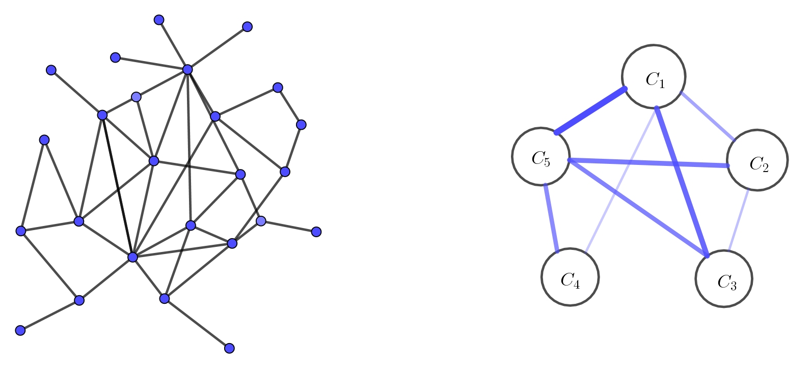
In this paper, we propose a summarization algorithm which, given an undirected graph , iteratively builds a summary, called reduced graph (Figure 1), defined as follows.
Definition 2 (Reduced graph).
Given an -regular partition
of a graph and , the reduced graph of is the undirected weighted graph , where , and is defined as follows:
We are now ready to state the Regularity Lemma which provides us a principled way to develop a summarization algorithm with the aim of separating structure from noise in a large graph.
3 Szemerédi’s Regularity Lemma
In essence, Szemerédi’s Regularity Lemma states that given an , every sufficiently dense graph can be approximated by the union of a bounded number of quasi-random bipartite graphs, where the deviation from randomness is controlled by the tolerance parameter . In other words, we can partition the vertex set into a bounded number of classes , such that almost every pair behaves similarly to a random bipartite graph, ().
Lemma 1 (Szemerédi’s regularity lemma ()).
For every positive real and for every positive integer , there are positive integers and with the following property: for every graph , with , there is an -regular partition of into classes such that .
The strength of the Regularity Lemma is corroborated by the so-called Key Lemma, which is an important theoretical result introduced by Komlos et al. [3]. It basically states that the reduced graph does inherit many of the essential structural properties of the original graph. Before presenting its original formulation, another kind of graph needs to be defined, namely the fold graph. Given an integer and a graph (which may be seen as a reduced graph), let denote the graph obtained by “blowing up” each vertex of to a set of independent vertices, and joining to if and only if is an edge in . Thus, is a graph in which every edge of is replaced by a copy of the complete bipartite graph . The following lemma shows a link between the reduced graph and .
Theorem 1 (Key Lemma).
Given , a graph , and a positive integer , let us construct a graph by performing the following steps:
-
1.
replace every vertex of by vertices;
-
2.
replace the edges of with -regular pairs of density at least .
Let be a subgraph of with vertices and maximum degree , and let and . If and , then is embeddable into (i.e. contains a subgraph isomorphic to ). In fact, we have:
| (3) |
where denotes the number of labeled copies of in .
Hence, the Key Lemma provides us a theoretical guarantee on the quality of the summary built from an -regular partition. In particular, for , , and if the constraint on the edge density is satisfied, the Key Lemma ensures that every small subgraph of is also a subgraph of . Thus, we can use the Regularity Lemma to build a summary of , and then we can infer structural properties of by studying the same properties on .
Finding Regular Partitions
The original proof of the Regularity Lemma is not constructive, but during the last decades different constructive versions have been proposed. In this paper, we focus on the Alon et al.’s [4] work. In particular, they proposed a new formulation of the Regularity Lemma which emphasizes the algorithmic nature of the result.
Theorem 2.
(Alon et al., 1994) For every and every positive integer there is an integer such that every graph with vertices has an -regular partition into classes, where . For every fixed and such partition can be found in sequential time, where is the time for multiplying two matrices with entries over the integers. It can also be found in time on an Exclusive Read Exclusive Write Parallel Random Access Machine(EREW PRAM) with a polynomial number of parallel processors.
A sketch of the proof is then presented. Let be a bipartite graph with color classes and , with . Let us define the average degree of as:
where is the degree of vertex .
For two distinct vertices the neighbourhood deviation of and is defined as:
where is the set of neighbours of vertex . For a subset the deviation of is defined as:
Let , it can be proved that, if there exists such that , then at least one of the following cases occurs:
-
1.
( is -regular);
-
2.
there exists in a set of more than vertices whose degrees deviate from by at least ( is -irregular);
-
3.
there are subsets such that ( is -irregular).
Note that one can easily check if 1 holds in time . Similarly, it is trivial to check if 2 holds in time, and in case it holds to exhibit the required subset of establishing this fact. If the first two conditions are not verified, the 3 condition must be checked. To this end, we have to find the subsets , called certificates, that witness the irregularity of the bipartite graph . To address this task, we first select a subset of whose vertex degrees “deviate” the most from the average degree of . More formally: for each with we find the vertex set . The proof provided by Alon et al. guarantees the existence of at least one such for which . Thus, the subsets and are the required certificates. These two subsets represent the collection of vertices that contribute more to the irregularity of the pair . The sets are called complements. Since the computation of the quantities , for , can be done by squaring the adjacency matrix of , the overall complexity of this algorithms is .
Before reporting Alon et al.’s algorithm, we present a measure to assess the goodness of a partition of the vertex set of a graph , which was introduced by Szemerédi [1]. Given a partition of a graph , the index (sze_idx) of the partition is defined as follows:
Since , it can be seen that . Szemerédi proved that if a partition violates the regularity condition, then it can be refined by a new partition such that . Finally, we can now present Alon et al.’s algorithm, which provides a way to find an -regular partition. The procedure is divided into two main steps: in the first step all the constants needed during the next computation are set; in the second one, the partition is iteratively created. An iteration is called refinement step, because, at each iteration, the current partition is closer to a regular one.
Alon et al.’s Algorithm
-
1.
Create the initial partition: arbitrarily divide the vertices of into an equitable partition with classes where .
-
2.
Check Regularity: for every pair of , verify if it is -regular or find two certificates such that .
-
3.
Count regular pairs: if there are at most pairs that are not -regular, then stop. is an -regular partition.
-
4.
Refine: apply a refinement algorithm and obtain a partition with classes, such that .
-
5.
Go to step 2.
Even if the above mentioned algorithm has polynomial worst case complexity in the size of , there is a hidden tower-type dependence on an accuracy parameter. Unfortunately, Gowers [21] proved that this tower function is necessary in order to guarantee a regular partition for all graphs. This implies that, in order to have a faithful approximation, the original graph size should be astronomically big. This has typically discouraged researchers from applying regular partitions to practical problems, thereby confining them to the purely theoretical realm.
To make the algorithm truly applicable, [9], and later [22, 7], instead of insisting on provably regular partitions, proposed a few simple heuristics that try to construct an approximately regular partition. In the next section, we present a new heuristic algorithm which is characterized by an improvement of the summary quality both in terms of reconstruction error and of noise filtering.
4 The Summarization Algorithm
The main limitations which prevent the application of Alon et al.’s algorithm to practical problems concern Step 2 and Step 4. In particular, in Step 2 the algorithm checks the regularity of all classes pairs by using the three conditions previously described. Given a pair , condition 1 verifies if it is -regular, otherwise conditions 2 and 3 are used to obtain the certificates and that witness the irregularity. The main obstacle concerning the implementation of condition 3 is the necessity to scan over almost all possible subsets of . To make the implementation of condition 3 feasible, given a class , we select in a greedy way a set with the highest deviation (the deviation is defined in 3). To do so, the nodes of are sorted by bipartite degree, and is built by adding nodes with the highest degree. At each iteration of the greedy algorithm, the node with a degree that deviates most from the average degree is added to the candidate certificate . This last operation is repeated until the subset , that satisfies condition 3, is found. This almost guarantees to put in the candidate certificate the nodes that have a connectivity pattern that deviates most from the one characterizing the majority of the nodes which belong to .
As far Step 4 is concerned, here an irregular partition is refined by a new partition , such that the partition index sze_idx is increased. This step poses the main obstacle towards a practical version of Alon et al.’s algorithm involving the creation of an exponentially large number of subclasses at each iteration. Indeed, as we have said, Step 2 finds all possible irregular pairs in the graph. As a consequence, each class may be involved with up to irregular pairs, being the number of classes in the current partition , thereby leading to an exponential growth. To avoid the problem, for each class, one can limit the number of irregular pairs containing it to at most one, possibly chosen randomly among all irregular pairs. This simple modification allows one to divide the classes into a constant, rather than exponential, number of subclasses (typically ). Despite the crude approximation this seems to work well in practice.
The devised algorithm takes as input two main parameters, the tolerant parameter and the minimum compression rate , that acts as a stopping criterion in the refinement process, and returns an approximated -regular partition. Its pseudocode is reported in Algorithm 1, where the procedure ApproxAlonCertificates, based on the two heuristics described above, takes as input a partition and returns the number of irregular pairs of . In the next paragraph, we describe the Refinement procedure which refines a partition into a partition . Its pseudocode is reported in Algorithm 2. The overall complexity of our summarization algorithm is , which is dominated by the verification of condition 3.
Given a partition , the Refinement procedure starts by randomly selecting a class , then iteratively processes all the others.
-
•
If is -regular with all the others, the procedure sorts the nodes of by their internal degree, i.e. the degree calculated with respect to the nodes of the same class, obtaining the following sorted sequence of nodes . The next step splits (Unzip) this sequence into two sets and . The latter sets are part of the refined partition .
-
•
If forms an irregular pair with other classes, the heuristic selects the candidate that shares the most similar internal structure with by maximizing , where is the internal density.
After selecting the best matching class , we are ready to split the pair in 4 new classes based on the internal densities of the certificates and .
-
–
In particular, a Sparsification procedure is applied when the internal density of a certificate is below a given threshold. This procedure randomly splits the certificate into two new classes. In order to match the equi-cardinality property, the new classes are filled up to by adding the remaining nodes from the corresponding complement. We choose the nodes that share the minimum number of connections with the new classes.
-
–
On the other hand, if the internal density of a certificate is above a given threshold, then a Densification procedure is applied. In particular, the heuristics sorts the nodes of the certificate by their internal degree and Unzip the set into two new classes. Also in this case, we fill the new sets up to by adding the remaining nodes from the corresponding complement by choosing the nodes which share the major number of connections with the new classes.
-
–
5 Graph Search Using Summaries
In this section, we discuss how to use our summarization framework to efficiently address the graph search problem defined under a similarity measure. The aim of graph search is to retrieve from a database the top- graphs that are most similar to a query graph.
Problem Definition
We consider a graph database containing a high number of simple undirected graphs , and, for the sake of generality, we allow the edges to be weighted.
Problem 1 (Graph search).
Given a graph database , a query graph , and a positive integer , the graph similarity search problem is to find the top- graphs in that are most similar to according to a similarity measure.
As far as the similarity measure is concerned, the most used one is the graph edit distance () due to its generality, broad applicability and noise robustness [17, 20]. However, since the computation is NP-hard, it is not suited to deal with large graphs. To overcome this limitation, we use the spectral distance [23], which is computed by comparing the eigenvalues of the two graphs being matched. The choice of this measure is motivated by the work of Van Dam and Haemers [24], who show that graphs with similar spectral properties generally share similar structural patterns. In this paper, we introduce a slightly modified version of the spectral distance to increase its range of applicability to pairs of graphs that violate the assumption of the Theorem 1 in [23], which assumes a precise order between the eigenvalues of the two graphs being matched. To this aim, we simply compute the absolute value of the difference between the - eigenvalue of the first graph with the - one of the second graph.
Definition 3 (Spectral distance).
Given two simple undirected weighted
graphs with , and with . Let us denote the corresponding spectra as and . We may assume without loss of generality that . The spectral distance is then defined as follows
| (4) |
where, controls which part of the spectra are being matched. In particular, eigenvalues of are compared with the head and tail eigenvalues of the .
Using The Summaries
In our approach, all the graphs contained in a database are summarized off-line, while the query graph is summarized on-line by means of our summarization framework. Thus, graph search can be performed on graph summaries, and this allows us to speed up the search process and to reduce the storage space. In particular, for each graph of a database , we store two different quantities: the summary of and the eigenvalues of . We then summarized on-line the query graph obtaining its summary . Finally, we compute the spectral distance between and each summary . The desired top- graphs will be obtained by selecting, from , the graphs corresponding to the smallest value of the spectral distance previously computed. The pseudocode of our approach to graph search is reported in Algorithm .
6 Experimental Evaluation
In this section, we evaluate our summarization algorithm both on synthetic graphs and on real-world networks to assess:
-
•
the ability of the proposed algorithm to separate structure from noise;
-
•
the usefulness of the summaries in retrieving from a database the top- graphs that are most similar to a query graph.
Experimental Settings
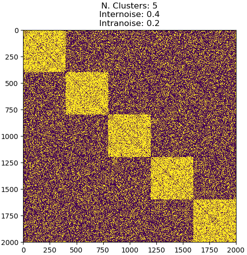
In our experiments we used both synthetic graphs and real-world networks. We generated synthetic graphs with a cluster structure, where the clusters are perturbed with different levels of noise. In particular, each graph is generated by adding spurious edges between cluster pairs and by dropping edges inside each cluster. Figure 2 provides a concrete example with a visual explanation. The pseudocode of the algorithm used to generate the synthetic datasets is reported in Algorithm 4.
As far as the real-world networks are concerned, we used two different datasets which have been taken from two famous repositories: the Stanford Large Network Dataset Collection SNAP [25] and the Konect repository of the University Koblenz-Landau Konect [26]. In particular, we used the following networks: Facebook [27], Email-Eu-core [28][29], Openflights[30], and Reactome [31]. Our algorithm is implemented in Python 222The implementation is available from https://github.com/MarcoFiorucci/graph-summarization-using-regular-partitions and the experiments are performed on an Intel Core i5 @ 2.60GHz HP Pavilion 15 Notebook with 8GB of RAM (DDR3 Synchronous 1600 MHz) running Arch-Linux with kernel version 4.14.4-1.
6.1 Graph Summarization
We performed experiments on both synthetic graphs and on real-world networks to assess the ability of the proposed algorithm to separate structure from noise. As evaluation criterion, we used the reconstruction error, which is expressed in terms of normalized norm computed between the similarity matrix of an input graph and the similarity matrix of the corresponding reconstructed graph .
Definition 4 (Reconstruction error).
Given the similarity matrix of the input graph and the similarity matrix of the reconstructed graph , the reconstruction error is defined as follows:
We decided to use the reconstruction error in order to compare our results with the ones presented by Riondato et al. [13], who evaluated the summary quality using this measure. This choice is due to the fact that their algorithm summarizes a graph by minimizing the reconstruction error. However, they pointed out that the reconstruction error has some shortcomings. In particular, given an unweighted graph , it is possible to produce an uninteresting summary with only one supenode corresponding to the vertex set and reconstruction error at most . On the other hand, if we obtained an useful summary, where each pair of vertices belonging to a supernode share an high number of common neighbors, then we get a low (say ) reconstruction error: this is a desirable behavior because low values of correspond to high quality summaries. Unfortunately, such low values are often obtained only with summaries having an high number of supernodes. This prevents to adopt the reconstruction error as a general measure to assess the summary quality.
As far the summarization and reconstruction steps are concerned, we proceeded, in all the experiments, in the following way: we applied our summarization algorithm (see Algorithm 1) to summarize an input graph . We then “blow-up” the summary in order to obtain the reconstructed graph , which preserves the main structure carried by the input graph (Figure 3).

Noise Robustness Evaluation
We study the ability of the proposed algorithm to separate structure from noise in graphs performing an extensive series of experiments on both synthetic graphs and real-world networks. As far synthetic graph experiments are concerned, we generated a graph by corrupting the clusters of in the following way: we added spurious edges between each cluster pair with probability , and we dropped edges inside each cluster with probability (see algorithm 4). As far as the real-world networks experiments are concerned, we added spurious edges with probability to a original graph obtaining an input graph .
In the ideal case, the distance between and the corresponding reconstructed graph should be only due to the filtered noise, while the distance between an should be closed to zero. Hence, we computed the reconstruction error to assess the robustness of our summarization framework against noise.
Experiment 1. We generated synthetic graphs of different sizes, spanning from up to nodes. We synthesized graphs by considering, for each of the different sizes, all the combinations of the following noise probabilities:
-
•
the probability of adding a spurious edge between a pair of clusters, called inter-cluster noise probability, which assumes values in ;
-
•
the probability of dropping an edge inside each cluster, called intra-cluster noise probability, which assumes values in .
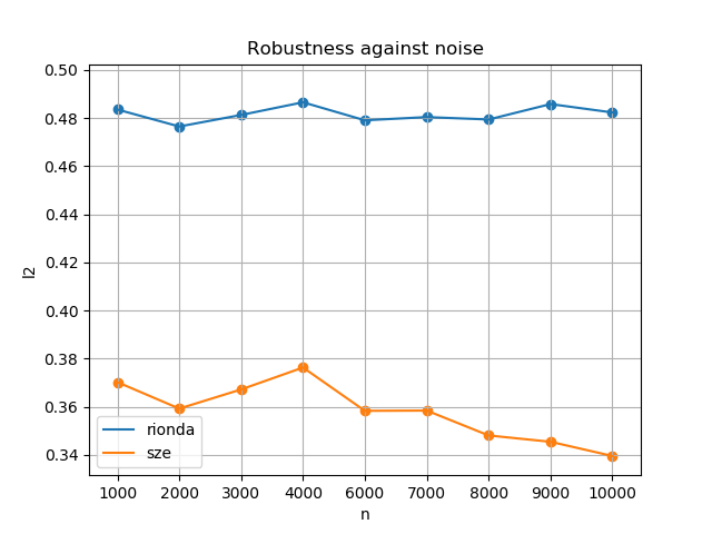
Let’s consider a synthetic graph , where n is its size, and corresponds to one of the pairs of noise probabilities. For each we obtained the reconstructed graph , and we then computed the reconstruction error . Given a size , we computed the median of
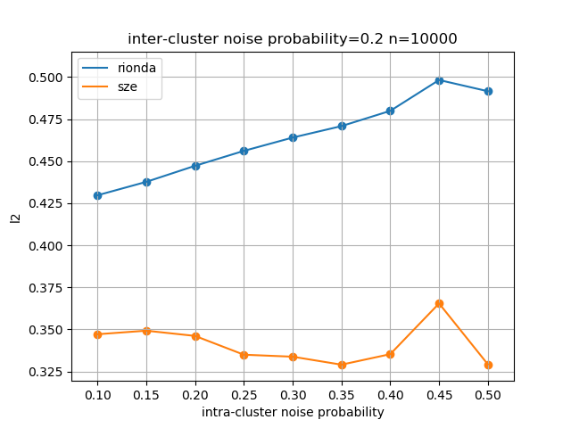
. We reported in figure 4 the medians computed using our summarization framework and the corresponding medians obtained by applying Riondato et al.’s algorithm [13]. We can see how our framework outperforms the state-of-the-art summarization algorithm in terms of robustness against noise.
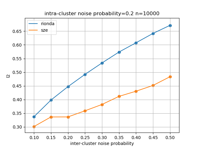
Experiment 2. The aim of this experiment is to study separately the robustness against the inter-cluster and the intra-cluster noise. Let’s consider the probability of dropping an edge inside each cluster equals to and the graph size equals to . To asses the inter-cluster noise robustness, we generated synthetic graphs , where assumes values in , and we computed the reconstruction errors . As far the intra-cluster noise is concerned, we chose the probability of adding a spurious edges between each pair of clusters , and the graph size . We then generated synthetic graphs , where assumes values in , and we computed the reconstruction errors .
Figure 5 illustrates the comparison between our results with those obtained by applying Riondato et al.’s algorithm [13]. This results are in accord to those presented in figure 4, and provides an experimental verification of the ability of our method to separate structure from noise in graphs.
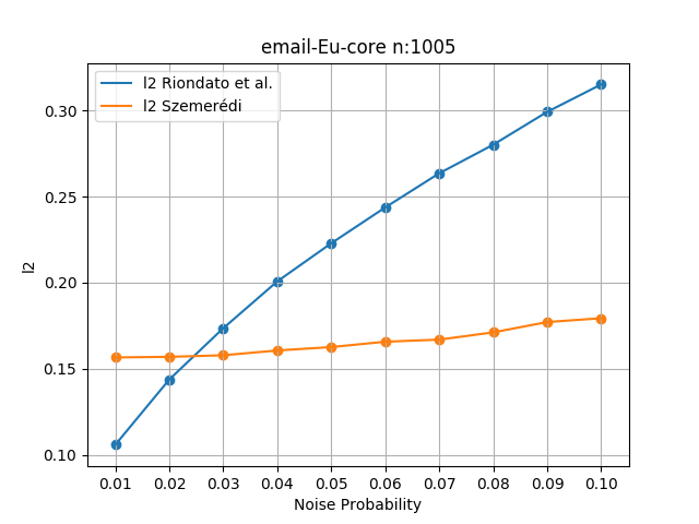
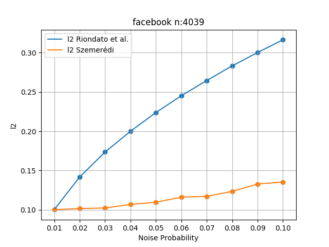
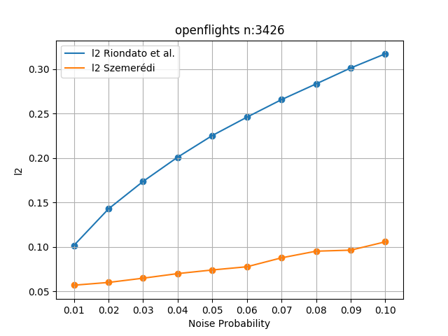
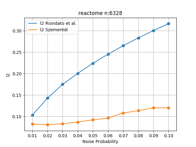
Experiment 3. We added spurious edges with probability to an original real-world network obtaining an input graph . The assumes values in . We applied this procedure on real-word networks, which have been taken from the Stanford Large Network Dataset Collection SNAP [25] and from the Konect repository of the University Koblenz-Landau Konect [26]. Since our framework is based on the Regularity Lemma, which is suited to deal only with dense graphs, we expect to obtain low quality summaries from sparse real-world networks. However, as shown in figure 6, our framework outperforms the state-of-the-art summarization algorithm in terms of robustness against noise providing good quality summary even on sparse real-world networks. In particular, we can see how the quality increases with the size of the input graph, which is in accord with the assumptions of the Regularity Lemma.
6.2 Graph Search
We performed extensive experiments on synthetic datasets to assess the usefulness of the summaries in retrieving, from a database, the top- graphs that are most similar to a query graph. To this end, we evaluate the quality of the answer in terms of the found top- similar graphs, and we evaluate the scalability both in the size of the database and in the size of the graphs.
Quality Evaluation
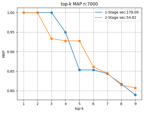
We conducted the following experiment: we compared graph search on the summaries with the baseline approach, in which the spectral distance is computed between no preprocessed graphs. The aim of the experiment is to show that pre-summarizing the graphs in the databases increases the noise robustness of the search process. We created a database contained synthetic graphs, which have different structures corrupting with different levels of noise (see algorithm 4). In particular, each graph is generated by combining the following three factors: five different possible number of clusters , six different possible levels of intra-cluster noise probability and six different possible levels of inter-cluster noise probability . Given a size , we generated graphs considering all the possible combinations of these three parameters. As described in Algorithm 3, we stored in the eigenvalues of the synthetic graphs, their summaries and the corresponding eigenvalues. Finally, we grouped the database graphs into five groups. Each group , with , is composed by 36 graphs that are generated by corrupting the same cluster structure with different combinations of intra-cluster and inter-cluster noise probability. Hence, all the graphs belonging to a given group are similar, since they have the same main structure.
More formally, we constructed a set of five query graphs by randomly sampling one graph from each group . Then, we first computed the spectral distance between and every graph in the database . We then calculated the for each query by considering relevant the graphs belonging to i.e. the same group of . Finally, we computed the score by averaging the average precision of the five graphs in .
We repeated the same procedure using the summaries of the synthetic graphs contained in . The aim of this experiment is to compare the quality obtained using our approach with that obtained by computing the spectral distance between original graphs.
We performed the experiment by considering the following graph sizes .
The and the are defined as follows.
Definition 5 (Average precision).
Given a query , a set of relevant graphs (graphs that share the same structure with ). Let us consider the output top- graphs in a database ordered by crescent spectral distance. We define the average precision at as follows.
| (5) |
where is the relevant proportion of the found top- graphs, while is if the considered graph is part of and is otherwise. Finally, is the number of relevant graphs.
Definition 6 (Mean average precision).
Given a query set , the mean average precision is defined as follows.
| (6) |
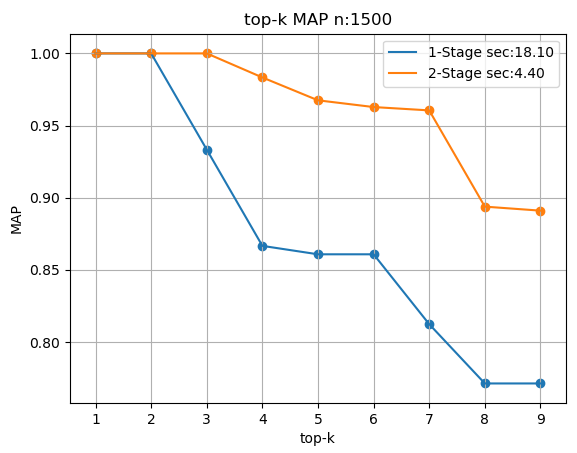
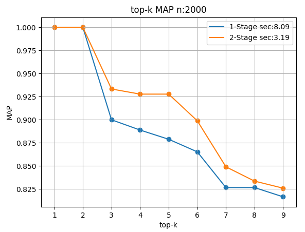
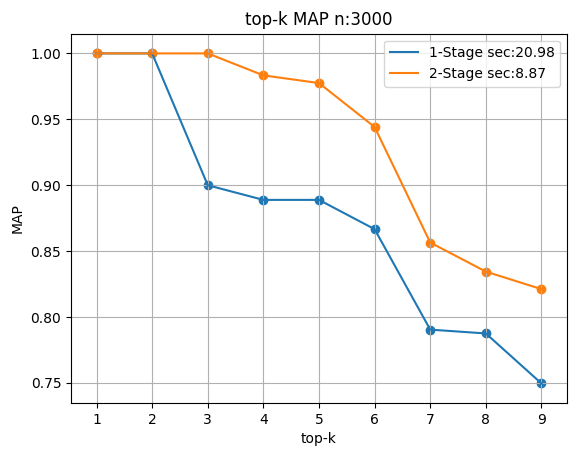
In particular, the higher is the value of the , the higher is the quality of the proposed graph search algorithm. Figures 7, 8, 9, 10 show that the proposed summarization based approach improved the query quality.
Scalability
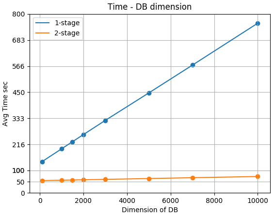
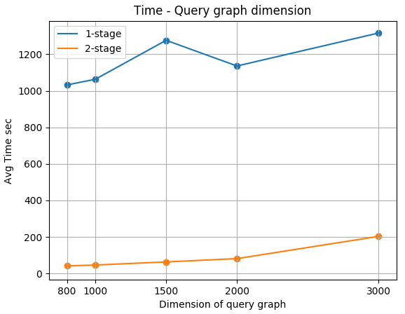
In order to evaluate the scalability of our approach, we conducted two different experiments. In the first one, we investigated the time required to perform a single query as the dimension of the database grows. In the second one, we investigated the query time in function of the size of the query graph.
In the first experiment, we fixed the size of all the graphs to be . We then generated the graphs in using all the possible combinations of the following factors: three different numbers of clusters , six different levels of intra-cluster noise probability , and six different levels of inter-cluster noise probability . The combination of these three parameters allow us to generate 108 graphs. We then copied them enough times to reach a database cardinality spanning from up to graphs.
The query time is calculated as follows:
| (7) |
where is the time required to obtain the summary of the query graph ; is the time required to calculate the eigenvectors of ; and is the time required to calculate the spectral distances between and each graph summary contained in . We reported in Figure 11, the computed time versus the cardinality of the database .
In the second experiment, we generated different databases , containing graphs. All the graphs in have the same size and have been created analogously as the previous experiment. We then constructed a query graph of the same size of the graphs in , and we measured the query time as we did for the previous experiment. We reported in Figure 12, the computed versus the size of the graph query . Figures 11, 12 provide us an experimental verification of the scalability of our approach both in the size of the database and in the size of the query graph.
7 Conclusions
In this work, we introduced a graph summarization approach based on the Regularity Lemma, which provides us with a principled way to describe the essential structure of large graphs using a small amount of data. We have successfully validated our framework both on synthetic and real-world graphs showing that our algorithm surpasses the state-of-the-art graph summarization methods in terms of noise robustness. In the second part of the paper, we presented an algorithm to address the graph similarity search problem exploiting our summaries. In particular, the proposed method is tailored for efficiently dealing with databases containing a high number of large graphs, and, moreover, it is robust against noise, which is always presented in real-world data. This achievement seems of particular interest since, to the best of our knowledge, we are the first to devise a graph search algorithm which satisfies all the above requirements together. A weak point of our summarization algorithm is related to its time complexity, which prevents the application of our framework to networks of millions of nodes. This demands for the development of efficient approaches suited to deal with large sparse graphs. In this direction, it would be a good idea to develop a heuristic based on the version of the Weak Regularity Lemma introduced by Fox et al. [32], as well as designing a distributed version of the regular decomposition algorithm introduced by Reittu et al. [33], who studied the linkage among the Regularity Lemma, the Stochastic Block Model and the Minimum Description Length. We think that the notion of regular partition will allow us to tackle the scalability issue faced by graph-based approaches [34, 35]. This would pave the way for a principled approach to massive network data analysis by combining modern graph theory and combinatorics with machine learning and pattern recognition.
References
References
- [1] E. Szemerédi, On sets of integers containing no k elements in arithmetic progression, Acta Arithm. 27 (1975) 199–245.
- [2] J. Komlós, A. Shokoufandeh, M. Simonovits, E. Szemerédi, The regularity lemma and its applications in graph theory, in: G. B. Khosrovshahi, A. Shokoufandeh, A. Shokrollahi (Eds.), Theoretical Aspects of Computer Science: Advanced Lectures, Springer, Berlin, 2002, pp. 84–112.
- [3] J. Komlos, M. Simonovits, Szemerédi’s Regularity Lemma and its applications in graph theory, DIMACS Technical Report.
- [4] N. Alon, R. Duke, H. Lefmann, V. Rodl, R. Yuster, The algorithmic aspects of the regularity lemma, Journal of Algorithms 16 (1) (1994) 80 – 109.
- [5] A. Czygrinow, V. Rödl, An algorithmic regularity lemma for hypergraphs, SIAM Journal on Computing 30 (4) (2000) 1041–1066.
- [6] A. M. Frieze, R. Kannan, A simple algorithm for constructing szemere’di’s regularity partition, Electr. J. Comb. 6.
- [7] M. Fiorucci, A. Torcinovich, M. Curado, F. Escolano, M. Pelillo, On the interplay between strong regularity and graph densification, in: Graph-Based Representations in Pattern Recognition - 11th IAPR-TC-15 International Workshop, GbRPR 2017, Anacapri, Italy, May 16-18, 2017, Proceedings, 2017, pp. 165–174.
- [8] M. Pelillo, I. Elezi, M. Fiorucci, Revealing structure in large graphs: Szemerédi’s regularity lemma and its use in pattern recognition, Pattern Recognition Letters 87 (2017) 4 – 11, advances in Graph-based Pattern Recognition.
- [9] A. Sperotto, M. Pelillo, Szemerédi’s regularity lemma and its applications to pairwise clustering and segmentation, in: Energy Minimization Methods in Computer Vision and Pattern Recognition, 6th International Conference, EMMCVPR 2007, Ezhou, China, August 27-29, 2007, Proceedings, 2007, pp. 13–27.
- [10] S. E. Schaeffer, Graph clustering, Computer Science Review 1 (1) (2007) 27 – 64.
- [11] M. E. J. Newman, M. Girvan, Finding and evaluating community structure in networks, Phys. Rev. E 69 (2) (2004) 026113.
- [12] K. LeFevre, E. Terzi, Grass: Graph structure summarization, Proceedings of the 2010 SIAM International Conference on Data Mining (2010) 454–465.
- [13] M. Riondato, D. García-Soriano, F. Bonchi, Graph summarization with quality guarantees, Data Min. Knowl. Discov. 31 (2) (2017) 314–349.
- [14] Y. Liu, A. Dighe, T. Safavi, D. Koutra, Graph Summarization: A Survey, ACM Computing Surveys V (N).
- [15] J. R. Ullmann, An algorithm for subgraph isomorphism, J. ACM 23 (1) (1976) 31–42.
- [16] V. Carletti, P. Foggia, A. Saggese, M. Vento, Challenging the time complexity of exact subgraph isomorphism for huge and dense graphs with vf3, IEEE Transactions on Pattern Analysis and Machine Intelligence 40 (4) (2018) 804–818.
- [17] Y. Liang, P. Zhao, Similarity search in graph databases: A multi-layered indexing approach, in: 2017 IEEE 33rd International Conference on Data Engineering (ICDE), 2017, pp. 783–794.
- [18] W. Zheng, L. Zou, X. Lian, D. Wang, D. Zhao, Efficient graph similarity search over large graph databases, IEEE Transactions on Knowledge and Data Engineering 27 (4) (2015) 964–978.
- [19] W. Zheng, L. Zou, X. Lian, D. Wang, D. Zhao, Graph similarity search with edit distance constraint in large graph databases, in: Proceedings of the 22Nd ACM International Conference on Information & Knowledge Management, CIKM ’13, ACM, 2013, pp. 1595–1600.
- [20] S. Zhang, J. Yang, W. Jin, Sapper: Subgraph indexing and approximate matching in large graphs, Proc. VLDB Endow. 3 (1-2) (2010) 1185–1194.
- [21] T. Gowers, Lower bounds of tower type for Szemerédi’s uniformity lemma, Geom Func. Anal. 7 (2) (1997) 322–337.
- [22] G. Sárközy, F. Song, E. Szemerédi, S. Trivedi, A prectical regularity partitioning algorithm and its applications in clustering, arXiv:1209.6540v1 [math.CO] (2012).
- [23] Y. Jin, J. F. JáJá, Network summarization with preserved spectral properties, CoRR abs/1802.04447.
- [24] E. R. van Dam, W. H. Haemers, Which graphs are determined by their spectrum?, Linear Algebra and its Applications 373 (2003) 241 – 272, combinatorial Matrix Theory Conference (Pohang, 2002).
- [25] J. Leskovec, A. Krevl, SNAP Datasets: Stanford large network dataset collection, http://snap.stanford.edu/data (Jun. 2014).
- [26] J. Kunegis, KONECT – The Koblenz Network Collection, in: Proc. Int. Conf. on World Wide Web Companion, 2013, pp. 1343–1350.
- [27] J. Leskovec, J. J. Mcauley, Learning to Discover Social Circles in Ego Networks, in: F. Pereira, C. J. C. Burges, L. Bottou, K. Q. Weinberger (Eds.), Advances in Neural Information Processing Systems 25, Curran Associates, Inc., 2012, pp. 539–547.
- [28] H. Yin, A. R. Benson, J. Leskovec, D. F. Gleich, Local Higher-Order Graph Clustering, in: Proceedings of the 23rd ACM SIGKDD International Conference on Knowledge Discovery and Data Mining - KDD ’17, 2017, pp. 555–564.
- [29] J. Leskovec, J. Kleinberg, C. Faloutsos, Graph Evolution: Densification and Shrinking Diameters, ACM Trans. Knowl. Discov. Data 1 (1).
- [30] Openflights network dataset – KONECT (Sep. 2016).
- [31] G. Joshi-Tope, M. Gillespie, I. Vastrik, P. D'Eustachio, E. Schmidt, B. de Bono, B. Jassal, G. R. Gopinath, G. R. Wu, L. Matthews, S. Lewis, E. Birney, L. Stein, Reactome: A knowledgebase of biological pathways, Nucleic Acids Research 33 (DATABASE ISS.).
- [32] J. Fox, L. M. Lovász, Y. Zhao, A fast new algorithm for weak graph regularity, CoRR abs/1801.05037 (2018) 1–13.
- [33] H. Reittu, L. Leskela, T. Raty, M. Fiorucci, Analysis of large sparse graphs using regular decomposition of graph distance matrices, in: 2018 IEEE International Conference on Big Data (Big Data), 2018, pp. 3784–3792.
- [34] H. Bunke, K. Riesen, Recent advances in graph-based pattern recognition with applications in document analysis, Pattern Recognition 44 (5) (2011) 1057 – 1067.
- [35] M. Vento, A long trip in the charming world of graphs for pattern recognition, Pattern Recogn. 48 (2) (2015) 291–301.