A numerical approach for solving fractional optimal control problems using modified hat functions

Somayeh Nemati s.nemati@umz.ac.ir, s.nemati@ua.pt Pedro M. Lima pedro.t.lima@ist.utl.pt Delfim F. M. Torres delfim@ua.pt Department of Mathematics, Faculty of Mathematical Sciences, University of Mazandaran, Babolsar, Iran Center for Research and Development in Mathematics and Applications (CIDMA),
Department of Mathematics, University of Aveiro, Aveiro 3810-193, Portugal
Centro de Matemática Computacional e Estocástica, Instituto Superior Técnico,
Universidade de Lisboa, Av. Rovisco Pais, 1049-001 Lisboa, Portugal
Abstract

We introduce a numerical method, based on modified hat functions, for solving a class of fractional optimal control problems. In our scheme, the control and the fractional derivative of the state function are considered as linear combinations of the modified hat functions. The fractional derivative is considered in the Caputo sense while the Riemann–Liouville integral operator is used to give approximations for the state function and some of its derivatives. To this aim, we use the fractional order integration operational matrix of the modified hat functions and some properties of the Caputo derivative and Riemann–Liouville integral operators. Using results of the considered basis functions, solving the fractional optimal control problem is reduced to the solution of a system of nonlinear algebraic equations. An error bound is proved for the approximate optimal value of the performance index obtained by the proposed method. The method is then generalized for solving a class of fractional optimal control problems with inequality constraints. The most important advantages of our method are easy implementation, simple operations, and elimination of numerical integration. Some illustrative examples are considered to demonstrate the effectiveness and accuracy of the proposed technique.

keywords:
Fractional optimal control problems , Modified hat functions , Operational matrix of fractional integration , Inequality constraints.
MSC:
[2010] 26A33 , 34A08 , 49M05.

1 Introduction

Optimal control theory allows us to choose control functions in a dynamical system to achieve a certain goal. The theory generalizes that of the classical calculus of variations and has found many applications in engineering, physics, economics, and life sciences [1, 2]. In 1996/97, motivated by nonconservative physical processes in mechanics, the subject was extended to the case in which derivatives and integrals are understood as fractional operators of arbitrary order [3, 4].

Fractional optimal control is nowadays an important research area, allowing to apply the power of variational methods to real systems [5, 6, 7]. It is an expanding branch of applied mathematics that attracts more and more attention, having been applied in transportation, electronic, chemical and biological systems [8]. Another applications of fractional optimal control problems are shown in [9]. Besides providing nontrivial generalizations of the classical theory, it opens doors to new and interesting modern scientific problems [10, 11]. Given the complexity of the problems, numerical methods are indispensable [12, 13, 14].

Recently, numerical methods based on modified hat functions have shown to provide an effective way for solving fractional differential equations [15, 16]. Here, for the first time in the literature, we introduce such a method for solving a general class of fractional optimal control problems. More precisely, in this work we begin by considering the following fractional optimal control problem (FOCP):

minJ=0tff(t,x(t),u(t))𝑑t𝐽superscriptsubscript0subscript𝑡𝑓𝑓𝑡𝑥𝑡𝑢𝑡differential-d𝑡\min~{}J=\int_{0}^{t_{f}}f(t,x(t),u(t))dt (1)

subject to the fractional dynamic system

Dαx(t)=g(t,x(t),Dα1x(t),Dα2x(t),,Dαkx(t),u(t)),m1<αm,formulae-sequencesuperscript𝐷𝛼𝑥𝑡𝑔𝑡𝑥𝑡superscript𝐷subscript𝛼1𝑥𝑡superscript𝐷subscript𝛼2𝑥𝑡superscript𝐷subscript𝛼𝑘𝑥𝑡𝑢𝑡𝑚1𝛼𝑚D^{\alpha}x(t)=g\left(t,x(t),D^{\alpha_{1}}x(t),D^{\alpha_{2}}x(t),\ldots,D^{\alpha_{k}}x(t),u(t)\right),\quad m-1<\alpha\leq m,\\ (2)

and the initial conditions

x(i)(0)=qi,i=0,1,,m1,formulae-sequencesuperscript𝑥𝑖0subscript𝑞𝑖𝑖01𝑚1x^{(i)}(0)=q_{i},\quad i=0,1,\ldots,m-1, (3)

where α>αk>>α2>α1>0𝛼subscript𝛼𝑘subscript𝛼2subscript𝛼10\alpha>\alpha_{k}>\ldots>\alpha_{2}>\alpha_{1}>0, Dαsuperscript𝐷𝛼D^{\alpha} denotes the (left) Caputo derivative of order α𝛼\alpha, x()𝑥x(\cdot) is the state function, u()𝑢u(\cdot) is the control function, J𝐽J is called the performance index, and f𝑓f and g𝑔g are given continuous functions. The aim of problem (1)–(3) consists in finding the optimal state and control functions that minimize the performance index. In this paper, a numerical method based on the modified hat functions is introduced for solving problem (1)–(3) and then the method is developed for FOCPs with inequality constraints. Because of the importance of fractional optimal control in applications, the numerical solution of FOCPs is crucial and our results can be very useful for many researchers.

The paper is organized as follows. In Section 2, some preliminaries of fractional calculus are reviewed and the basis functions and their properties are presented. A numerical method for solving the FOCP (1)–(3) is introduced in Section 3. In Section 4, an error estimate is proved for the proposed method. Section 5 is devoted to the development of the method to solve constrained FOCPs. In Section 6, some FOCPs are considered and solved using the proposed method. Finally, a conclusion is given in Section 7.

2 Preliminaries

In this section, a brief review on necessary definitions and properties of fractional calculus is presented. Furthermore, the modified hat functions and some of their properties are recalled.

2.1 Preliminaries of fractional calculus

We use fractional derivatives in the sense of Caputo. They are defined via Riemann–Liouville fractional integral.

Definition 2.1 (See, e.g., [17]).

The Riemann–Liouville fractional integral operator with order α0𝛼0\alpha\geq 0 of a given function x()𝑥x(\cdot) is defined as

Iαx(t)=1Γ(α)0t(ts)α1x(s)𝑑s,I0x(t)=x(t),formulae-sequencesuperscript𝐼𝛼𝑥𝑡1Γ𝛼superscriptsubscript0𝑡superscript𝑡𝑠𝛼1𝑥𝑠differential-d𝑠superscript𝐼0𝑥𝑡𝑥𝑡\begin{split}&I^{\alpha}x(t)=\frac{1}{\Gamma(\alpha)}\int_{0}^{t}(t-s)^{\alpha-1}x(s)ds,\\ &I^{0}x(t)=x(t),\end{split}

where Γ()Γ\Gamma(\cdot) is the Euler gamma function.

Definition 2.2 (See, e.g., [17]).

The Caputo fractional derivative of order α>0𝛼0\alpha>0 of a function x()𝑥x(\cdot) is defined as

Dαx(t)=1Γ(mα)0t(ts)mα1x(m)(s)𝑑s,m1<αm.formulae-sequencesuperscript𝐷𝛼𝑥𝑡1Γ𝑚𝛼superscriptsubscript0𝑡superscript𝑡𝑠𝑚𝛼1superscript𝑥𝑚𝑠differential-d𝑠𝑚1𝛼𝑚D^{\alpha}x(t)=\frac{1}{\Gamma(m-\alpha)}\int_{0}^{t}(t-s)^{m-\alpha-1}x^{(m)}(s)ds,\quad m-1<\alpha\leq m.

For m1<αm𝑚1𝛼𝑚m-1<\alpha\leq m, m𝑚m\in\mathbb{N}, some useful properties of the Caputo derivative and Riemann–Liouville integral are as follows:

DαIαx(t)=x(t),superscript𝐷𝛼superscript𝐼𝛼𝑥𝑡𝑥𝑡D^{\alpha}I^{\alpha}x(t)=x(t),
IαDαx(t)=x(t)i=0m1x(i)(0)tii!,t>0,formulae-sequencesuperscript𝐼𝛼superscript𝐷𝛼𝑥𝑡𝑥𝑡superscriptsubscript𝑖0𝑚1superscript𝑥𝑖0superscript𝑡𝑖𝑖𝑡0I^{\alpha}D^{\alpha}x(t)=x(t)-\sum_{i=0}^{m-1}x^{(i)}(0)\frac{t^{i}}{i!},\quad t>0, (4)
IαβDαx(t)=Dβx(t)i=βm1x(i)(0)tiβΓ(iβ+1),0<β<α,t>0,formulae-sequenceformulae-sequencesuperscript𝐼𝛼𝛽superscript𝐷𝛼𝑥𝑡superscript𝐷𝛽𝑥𝑡superscriptsubscript𝑖𝛽𝑚1superscript𝑥𝑖0superscript𝑡𝑖𝛽Γ𝑖𝛽10𝛽𝛼𝑡0I^{\alpha-\beta}D^{\alpha}x(t)=D^{\beta}x(t)-\sum_{i=\lceil\beta\rceil}^{m-1}x^{(i)}(0)\frac{t^{i-\beta}}{\Gamma(i-\beta+1)},\quad 0<\beta<\alpha,\quad t>0, (5)

where \lceil\cdot\rceil is the ceiling function.

2.2 Properties of the modified hat functions

By considering an even integer number n𝑛n, the interval [0,tf]0subscript𝑡𝑓[0,t_{f}] is divided into n𝑛n subintervals [ih,(i+1)h]𝑖𝑖1[ih,(i+1)h], i=0,1,2,,n1𝑖012𝑛1i=0,1,2,\ldots,n-1, with h=tfnsubscript𝑡𝑓𝑛h=\frac{t_{f}}{n}. Then the generalized modified hat functions consist of a set of n+1𝑛1n+1 linearly independent functions in L2[0,tf]superscript𝐿20subscript𝑡𝑓L^{2}[0,t_{f}] that are defined as follows [15, 16]:

ψ0(t)={12h2(th)(t2h),0t2h,0,otherwise;subscript𝜓0𝑡cases12superscript2𝑡𝑡20𝑡2missing-subexpressionmissing-subexpression0otherwise\psi_{0}(t)=\left\{\begin{array}[]{ll}\frac{1}{2h^{2}}(t-h)(t-2h),&0\leq t\leq 2h,\\ &\\ 0,&\text{otherwise};\end{array}\right.

if i𝑖i is odd and 1in11𝑖𝑛11\leq i\leq n-1,

ψi(t)={1h2(t(i1)h)(t(i+1)h),(i1)ht(i+1)h,0,otherwise;subscript𝜓𝑖𝑡cases1superscript2𝑡𝑖1𝑡𝑖1𝑖1𝑡𝑖1missing-subexpressionmissing-subexpression0otherwise\psi_{i}(t)=\left\{\begin{array}[]{ll}\frac{-1}{h^{2}}(t-(i-1)h)(t-(i+1)h),&(i-1)h\leq t\leq(i+1)h,\\ &\\ 0,&\text{otherwise};\end{array}\right.

if i𝑖i is even and 2in22𝑖𝑛22\leq i\leq n-2,

ψi(t)={12h2(t(i1)h)(t(i2)h),(i2)htih,12h2(t(i+1)h)(t(i+2)h),iht(i+2)h,0,otherwise,subscript𝜓𝑖𝑡cases12superscript2𝑡𝑖1𝑡𝑖2𝑖2𝑡𝑖missing-subexpressionmissing-subexpression12superscript2𝑡𝑖1𝑡𝑖2𝑖𝑡𝑖2missing-subexpressionmissing-subexpression0otherwise\psi_{i}(t)=\left\{\begin{array}[]{ll}\frac{1}{2h^{2}}(t-(i-1)h)(t-(i-2)h),&(i-2)h\leq t\leq ih,\\ &\\ \frac{1}{2h^{2}}(t-(i+1)h)(t-(i+2)h),&ih\leq t\leq(i+2)h,\\ &\\ 0,&\text{otherwise},\end{array}\right.

and

ψn(t)={12h2(t(tfh))(t(tf2h)),tf2httf,0,otherwise.subscript𝜓𝑛𝑡cases12superscript2𝑡subscript𝑡𝑓𝑡subscript𝑡𝑓2subscript𝑡𝑓2𝑡subscript𝑡𝑓missing-subexpressionmissing-subexpression0otherwise\psi_{n}(t)=\left\{\begin{array}[]{ll}\frac{1}{2h^{2}}(t-(t_{f}-h))(t-(t_{f}-2h)),&t_{f}-2h\leq t\leq t_{f},\\ &\\ 0,&\text{otherwise}.\end{array}\right.

These functions satisfy some interesting properties, which make them very useful. Some of these properties are as follows:

ψi(jh)={1,i=j,0,ij,subscript𝜓𝑖𝑗cases1𝑖𝑗missing-subexpressionmissing-subexpression0𝑖𝑗\psi_{i}(jh)=\left\{\begin{array}[]{ll}1,&i=j,\\ &\\ 0,&i\neq j,\end{array}\right.
i=0nψi(t)=1,superscriptsubscript𝑖0𝑛subscript𝜓𝑖𝑡1\sum_{i=0}^{n}\psi_{i}(t)=1,
0tfψi(t)𝑑t={h3,if i=0,n,4h3if i is odd and 1in1,2h3,if i is even and 2in2.superscriptsubscript0subscript𝑡𝑓subscript𝜓𝑖𝑡differential-d𝑡cases3if i=0,nmissing-subexpressionmissing-subexpression43if i is odd and 1in1missing-subexpressionmissing-subexpression23if i is even and 2in2\int_{0}^{t_{f}}\psi_{i}(t)dt=\left\{\begin{array}[]{ll}\frac{h}{3},&\text{if $i=0,n$},\\ &\\ \frac{4h}{3}&\text{if $i$ is odd and $1\leq i\leq n-1$},\\ &\\ \frac{2h}{3},&\text{if $i$ is even and $2\leq i\leq n-2$}.\end{array}\right. (6)

Any function x()L2[0,tf]𝑥superscript𝐿20subscript𝑡𝑓x(\cdot)\in L^{2}[0,t_{f}] can be approximated using the modified hat functions as

x(t)xn(t)=i=0naiψi(t)=ATΨ(t),similar-to-or-equals𝑥𝑡subscript𝑥𝑛𝑡superscriptsubscript𝑖0𝑛subscript𝑎𝑖subscript𝜓𝑖𝑡superscript𝐴𝑇Ψ𝑡x(t)\simeq x_{n}(t)=\sum_{i=0}^{n}a_{i}\psi_{i}(t)=A^{T}\Psi(t), (7)

where

Ψ(t)=[ψ0(t),ψ1(t),,ψn(t)]T,Ψ𝑡superscriptsubscript𝜓0𝑡subscript𝜓1𝑡subscript𝜓𝑛𝑡𝑇\Psi(t)=[\psi_{0}(t),\psi_{1}(t),\ldots,\psi_{n}(t)]^{T}, (8)

and

A=[a0,a1,,an]T,𝐴superscriptsubscript𝑎0subscript𝑎1subscript𝑎𝑛𝑇A=[a_{0},a_{1},\ldots,a_{n}]^{T},

with ai=x(ih)subscript𝑎𝑖𝑥𝑖a_{i}=x(ih).

Let Ψ()Ψ\Psi(\cdot) be the modified hat functions basis vector given by (8) and α>0𝛼0\alpha>0. Then,

IαΨ(t)P(α)Ψ(t),similar-to-or-equalssuperscript𝐼𝛼Ψ𝑡superscript𝑃𝛼Ψ𝑡I^{\alpha}\Psi(t)\simeq P^{(\alpha)}\Psi(t), (9)

where P(α)superscript𝑃𝛼P^{(\alpha)} is a matrix of dimension (n+1)×(n+1)𝑛1𝑛1(n+1)\times(n+1) called the operational matrix of fractional integration of order α𝛼\alpha. This matrix is given (see [15, 16]) as

P(α)=hα2Γ(α+3)[0β1β2β3β4βn1βn0η0η1η2η3ηn2ηn10ξ1ξ0ξ1ξ2ξn3ξn2000η0η1ηn4ηn3000ξ1ξ0ξn5ξn400000η0η100000ξ1ξ0]superscript𝑃𝛼superscript𝛼2Γ𝛼3delimited-[]0subscript𝛽1subscript𝛽2subscript𝛽3subscript𝛽4subscript𝛽𝑛1subscript𝛽𝑛0subscript𝜂0subscript𝜂1subscript𝜂2subscript𝜂3subscript𝜂𝑛2subscript𝜂𝑛10subscript𝜉1subscript𝜉0subscript𝜉1subscript𝜉2subscript𝜉𝑛3subscript𝜉𝑛2000subscript𝜂0subscript𝜂1subscript𝜂𝑛4subscript𝜂𝑛3000subscript𝜉1subscript𝜉0subscript𝜉𝑛5subscript𝜉𝑛4missing-subexpression00000subscript𝜂0subscript𝜂100000subscript𝜉1subscript𝜉0P^{(\alpha)}=\frac{h^{\alpha}}{2\Gamma(\alpha+3)}\left[\begin{array}[]{cccccccc}0&\beta_{1}&\beta_{2}&\beta_{3}&\beta_{4}&\ldots&\beta_{n-1}&\beta_{n}\\ 0&\eta_{0}&\eta_{1}&\eta_{2}&\eta_{3}&\ldots&\eta_{n-2}&\eta_{n-1}\\ 0&\xi_{-1}&\xi_{0}&\xi_{1}&\xi_{2}&\ldots&\xi_{n-3}&\xi_{n-2}\\ 0&0&0&\eta_{0}&\eta_{1}&\ldots&\eta_{n-4}&\eta_{n-3}\\ 0&0&0&\xi_{-1}&\xi_{0}&\ldots&\xi_{n-5}&\xi_{n-4}\\ \vdots&\vdots&\vdots&\vdots&\vdots&&\vdots&\vdots\\ 0&0&0&0&0&\ldots&\eta_{0}&\eta_{1}\\ 0&0&0&0&0&\ldots&\xi_{-1}&\xi_{0}\\ \end{array}\right] (10)

with

β1=α(3+2α),βi=iα+1(2i63α)+2iα(1+α)(2+α)(i2)α+1(2i2+α),i=2,3,,n,η0=4(1+α),ηi=4[(i1)α+1(i+1+α)(i+1)α+1(i1α)],i=1,2,,n1,ξ1=α,ξ0=2α+1(2α),ξ1=3α+1(4α)6(2+α),ξi=(i+2)α+1(2i+2α)6iα+1(2+α)(i2)α+1(2i2+α),i=2,3,,n2.\begin{split}&\beta_{1}=\alpha(3+2\alpha),\\ &\beta_{i}=i^{\alpha+1}(2i-6-3\alpha)+2i^{\alpha}(1+\alpha)(2+\alpha)-(i-2)^{\alpha+1}(2i-2+\alpha),\quad i=2,3,\ldots,n,\\ &\eta_{0}=4(1+\alpha),\\ &\eta_{i}=4[(i-1)^{\alpha+1}(i+1+\alpha)-(i+1)^{\alpha+1}(i-1-\alpha)],~{}~{}i=1,2,\ldots,n-1,\\ &\xi_{-1}=-\alpha,\\ &\xi_{0}=2^{\alpha+1}(2-\alpha),\\ &\xi_{1}=3^{\alpha+1}(4-\alpha)-6(2+\alpha),\\ &\xi_{i}=(i+2)^{\alpha+1}(2i+2-\alpha)-6i^{\alpha+1}(2+\alpha)-(i-2)^{\alpha+1}(2i-2+\alpha),\quad i=2,3,\ldots,n-2.\end{split}

3 Numerical solution of problem (1)–(3)

In this section, we introduce a new numerical scheme for solving the optimal control problem (1)–(3). Our method is based on the properties of the modified hat functions. We begin by expanding the variable t𝑡t in terms of the modified hat functions. Using (7), this variable can then be rewritten as

t=ΘTΨ(t),𝑡superscriptΘ𝑇Ψ𝑡t=\Theta^{T}\Psi(t), (11)

where

Θ=[0,h,2h,,tf]T.Θsuperscript02subscript𝑡𝑓𝑇\Theta=[0,h,2h,\ldots,t_{f}]^{T}. (12)

Let us suppose that

Dαx(t)=ATΨ(t)superscript𝐷𝛼𝑥𝑡superscript𝐴𝑇Ψ𝑡D^{\alpha}x(t)=A^{T}\Psi(t) (13)

and

u(t)un(t)=UTΨ(t),similar-to-or-equals𝑢𝑡subscript𝑢𝑛𝑡superscript𝑈𝑇Ψ𝑡u(t)\simeq u_{n}(t)=U^{T}\Psi(t), (14)

where

A=[a0,a1,,an]T,U=[u0,u1,,un]T,formulae-sequence𝐴superscriptsubscript𝑎0subscript𝑎1subscript𝑎𝑛𝑇𝑈superscriptsubscript𝑢0subscript𝑢1subscript𝑢𝑛𝑇A=[a_{0},a_{1},\ldots,a_{n}]^{T},\quad U=[u_{0},u_{1},\ldots,u_{n}]^{T},

such that the elements of A𝐴A and U𝑈U are unknown. By utilizing (5), (9), (13), and the initial conditions given in (3), for s=1,2,,k𝑠12𝑘s=1,2,\ldots,k, we obtain that

Dαsx(t)=Iααs(Dαx(t))+i=αsm1x(i)(0)tiαsΓ(jαs+1)ATIααsΨ(t)+i=αsm1qitiαsΓ(iαs+1)(ATP(ααs)+DsT)Ψ(t)=XsTΨ(t),superscript𝐷subscript𝛼𝑠𝑥𝑡superscript𝐼𝛼subscript𝛼𝑠superscript𝐷𝛼𝑥𝑡superscriptsubscript𝑖subscript𝛼𝑠𝑚1superscript𝑥𝑖0superscript𝑡𝑖subscript𝛼𝑠Γ𝑗subscript𝛼𝑠1similar-to-or-equalssuperscript𝐴𝑇superscript𝐼𝛼subscript𝛼𝑠Ψ𝑡superscriptsubscript𝑖subscript𝛼𝑠𝑚1subscript𝑞𝑖superscript𝑡𝑖subscript𝛼𝑠Γ𝑖subscript𝛼𝑠1similar-to-or-equalssuperscript𝐴𝑇superscript𝑃𝛼subscript𝛼𝑠superscriptsubscript𝐷𝑠𝑇Ψ𝑡superscriptsubscript𝑋𝑠𝑇Ψ𝑡\begin{split}D^{\alpha_{s}}x(t)&=I^{\alpha-\alpha_{s}}(D^{\alpha}x(t))+\sum_{i=\lceil\alpha_{s}\rceil}^{m-1}x^{(i)}(0)\frac{t^{i-\alpha_{s}}}{\Gamma(j-\alpha_{s}+1)}\\ &\simeq A^{T}I^{\alpha-\alpha_{s}}\Psi(t)+\sum_{i=\lceil\alpha_{s}\rceil}^{m-1}q_{i}\frac{t^{i-\alpha_{s}}}{\Gamma(i-\alpha_{s}+1)}\\ &\simeq(A^{T}P^{(\alpha-\alpha_{s})}+D_{s}^{T})\Psi(t)\\ &=X_{s}^{T}\Psi(t),\end{split} (15)

where we have used the notations

i=αsm1qitiαsΓ(iαs+1)DsTΨ(t),Xs=(ATP(ααs)+DsT)Tformulae-sequencesimilar-to-or-equalssuperscriptsubscript𝑖subscript𝛼𝑠𝑚1subscript𝑞𝑖superscript𝑡𝑖subscript𝛼𝑠Γ𝑖subscript𝛼𝑠1superscriptsubscript𝐷𝑠𝑇Ψ𝑡subscript𝑋𝑠superscriptsuperscript𝐴𝑇superscript𝑃𝛼subscript𝛼𝑠superscriptsubscript𝐷𝑠𝑇𝑇\sum_{i=\lceil\alpha_{s}\rceil}^{m-1}q_{i}\frac{t^{i-\alpha_{s}}}{\Gamma(i-\alpha_{s}+1)}\simeq D_{s}^{T}\Psi(t),\quad X_{s}=(A^{T}P^{(\alpha-\alpha_{s})}+D_{s}^{T})^{T}

with

Xs=[xs,0,xs,1,,xs,n]T.subscript𝑋𝑠superscriptsubscript𝑥𝑠0subscript𝑥𝑠1subscript𝑥𝑠𝑛𝑇X_{s}=[x_{s,0},x_{s,1},\ldots,x_{s,n}]^{T}.

Furthermore, the state function can be approximated using (4), (9), and (13), as

x(t)xn(t)=XTΨ(t),similar-to-or-equals𝑥𝑡subscript𝑥𝑛𝑡superscript𝑋𝑇Ψ𝑡x(t)\simeq x_{n}(t)=X^{T}\Psi(t), (16)

where we have used

i=0m1qitii!DTΨ(t),X=(ATP(α)+DT)Tformulae-sequencesimilar-to-or-equalssuperscriptsubscript𝑖0𝑚1subscript𝑞𝑖superscript𝑡𝑖𝑖superscript𝐷𝑇Ψ𝑡𝑋superscriptsuperscript𝐴𝑇superscript𝑃𝛼superscript𝐷𝑇𝑇\sum_{i=0}^{m-1}q_{i}\frac{t^{i}}{i!}\simeq D^{T}\Psi(t),\quad X=(A^{T}P^{(\alpha)}+D^{T})^{T} (17)

with

X=[x0,x1,,xn]T.𝑋superscriptsubscript𝑥0subscript𝑥1subscript𝑥𝑛𝑇X=[x_{0},x_{1},\ldots,x_{n}]^{T}.

We rewrite the elements of the vectors X𝑋X and Xssubscript𝑋𝑠X_{s}, s=1,2,,k𝑠12𝑘s=1,2,\ldots,k, in terms of the elements of the vector A𝐴A. To this aim, suppose that

P(ααs)=[pijs]i,j=0,1,,n,s=1,2,,k,P(α)=[pij]i,j=0,1,,n.\begin{split}&P^{(\alpha-\alpha_{s})}=[p_{ij}^{s}]_{i,j=0,1,\ldots,n},\quad\quad s=1,2,\ldots,k,\\ &P^{(\alpha)}=[p_{ij}]_{i,j=0,1,\ldots,n}.\end{split}

Taking into consideration (10), we have

pi0=pi0s=0,for i=0,1,2,,n,pij=pijs=0,for j=1,3,5,,n1, i=j+2,j+3,,n,pij=pijs=0,for j=2,4,6,,n, i=j+1,j+2,,n.\begin{split}&p_{i0}=p_{i0}^{s}=0,\quad\text{for $i=0,1,2,\ldots,n$},\\ &p_{ij}=p_{ij}^{s}=0,\quad\text{for $j=1,3,5,\ldots,n-1,$ $i=j+2,j+3,\ldots,n$},\\ &p_{ij}=p_{ij}^{s}=0,\quad\text{for $j=2,4,6,\ldots,n,$ $i=j+1,j+2,\ldots,n$}.\end{split}

Therefore, the entries xjsubscript𝑥𝑗x_{j} and xs,jsubscript𝑥𝑠𝑗x_{s,j} can be written in details as

x0=q0,xj=i=0j+1aipij+i=0m1qi(jh)ii!,j=1,3,,n1,xj=i=0jaipij+i=0m1qi(jh)ii!,j=2,4,,n,\begin{split}&x_{0}=q_{0},\\ &x_{j}=\sum_{i=0}^{j+1}a_{i}p_{ij}+\sum_{i=0}^{m-1}q_{i}\frac{(jh)^{i}}{i!},\quad j=1,3,\ldots,n-1,\\ &x_{j}=\sum_{i=0}^{j}a_{i}p_{ij}+\sum_{i=0}^{m-1}q_{i}\frac{(jh)^{i}}{i!},\quad j=2,4,\ldots,n,\\ \end{split}
xs,j=i=0j+1aipijs+i=αsm1qi(jh)iαsΓ(iαs+1),j=1,3,,n1,xs,j=i=0jaipijs+i=αsm1qi(jh)iαsΓ(iαs+1),j=2,4,,n.\begin{split}&x_{s,j}=\sum_{i=0}^{j+1}a_{i}p_{ij}^{s}+\sum_{i=\lceil\alpha_{s}\rceil}^{m-1}q_{i}\frac{(jh)^{i-\alpha_{s}}}{\Gamma(i-\alpha_{s}+1)},\quad j=1,3,\ldots,n-1,\\ &x_{s,j}=\sum_{i=0}^{j}a_{i}p_{ij}^{s}+\sum_{i=\lceil\alpha_{s}\rceil}^{m-1}q_{i}\frac{(jh)^{i-\alpha_{s}}}{\Gamma(i-\alpha_{s}+1)},\quad j=2,4,\ldots,n.\\ \end{split}

We employ the approximations given above in order to obtain an approximation of the performance index. For the function f:3:𝑓superscript3f:\mathbb{R}^{3}\rightarrow\mathbb{R}, using (7), (11), (14), and (16), we can write

f(t,x(t),u(t))i=0nf(ih,x(ih),u(ih))ψi(t)i=0nf(ih,xi,ui)ψi(t)=f(Θ,X,U)Ψ(t),similar-to-or-equals𝑓𝑡𝑥𝑡𝑢𝑡superscriptsubscript𝑖0𝑛𝑓𝑖𝑥𝑖𝑢𝑖subscript𝜓𝑖𝑡similar-to-or-equalssuperscriptsubscript𝑖0𝑛𝑓𝑖subscript𝑥𝑖subscript𝑢𝑖subscript𝜓𝑖𝑡𝑓Θ𝑋𝑈Ψ𝑡\begin{split}f(t,x(t),u(t))&\simeq\sum_{i=0}^{n}f(ih,x(ih),u(ih))\psi_{i}(t)\\ &\simeq\sum_{i=0}^{n}f(ih,x_{i},u_{i})\psi_{i}(t)\\ &=f(\Theta,X,U)\Psi(t),\\ \end{split} (18)

where

f(Θ,X,U)=[f(0,x0,u0),f(h,x1,u1),,f(tf,xn,un)].𝑓Θ𝑋𝑈𝑓0subscript𝑥0subscript𝑢0𝑓subscript𝑥1subscript𝑢1𝑓subscript𝑡𝑓subscript𝑥𝑛subscript𝑢𝑛f(\Theta,X,U)=[f(0,x_{0},u_{0}),f(h,x_{1},u_{1}),\ldots,f(t_{f},x_{n},u_{n})].

By substituting (18) into the performance index and employing (6), we obtain that

J0tff(Θ,X,U)Ψ(t)𝑑t=f(Θ,X,U)0tfΨ(t)𝑑t=f(Θ,X,U)L,similar-to-or-equals𝐽superscriptsubscript0subscript𝑡𝑓𝑓Θ𝑋𝑈Ψ𝑡differential-d𝑡𝑓Θ𝑋𝑈superscriptsubscript0subscript𝑡𝑓Ψ𝑡differential-d𝑡𝑓Θ𝑋𝑈𝐿J\simeq\int_{0}^{t_{f}}f(\Theta,X,U)\Psi(t)dt=f(\Theta,X,U)\int_{0}^{t_{f}}\Psi(t)dt=f(\Theta,X,U)L, (19)

where

L=h3[1,4,2,4,2,,2,4,1]T.𝐿3superscript14242241𝑇L=\frac{h}{3}\left[1,4,2,4,2,\ldots,2,4,1\right]^{T}. (20)

In a similar way, taking into account (7), (11), and (14)–(16) for the function g:k+3:𝑔superscript𝑘3g:\mathbb{R}^{k+3}\rightarrow\mathbb{R}, we have

g(t,x(t),Dα1x(t),,Dαkx(t),u(t))i=0ng(ih,x(ih),Dα1x(ih),,Dαkx(ih),u(ih))ψi(t)i=0ng(ih,xi,x1,i,,xk,i,ui)ψi(t)=g(Θ,X,X1,,Xk,U)Ψ(t),\begin{split}g(t,x(t),D^{\alpha_{1}}x(t),\ldots,D^{\alpha_{k}}x(t),u(t))&\simeq\sum_{i=0}^{n}g\left(ih,x(ih),D^{\alpha_{1}}x(ih),\right.\\ &\left.\quad\ldots,D^{\alpha_{k}}x(ih),u(ih)\right)\psi_{i}(t)\\ &\simeq\sum_{i=0}^{n}g\left(ih,x_{i},x_{1,i},\ldots,x_{k,i},u_{i}\right)\psi_{i}(t)\\ &=g(\Theta,X,X_{1},\ldots,X_{k},U)\Psi(t),\end{split} (21)

where

g(Θ,X,X1,,Xk,U)=[g(0,x0,x1,0,,xk,0,u0),g(h,x1,x1,1,,xk,1,u1),,g(tf,xn,x1,n,,xk,n,un)].𝑔Θ𝑋subscript𝑋1subscript𝑋𝑘𝑈𝑔0subscript𝑥0subscript𝑥10subscript𝑥𝑘0subscript𝑢0𝑔subscript𝑥1subscript𝑥11subscript𝑥𝑘1subscript𝑢1𝑔subscript𝑡𝑓subscript𝑥𝑛subscript𝑥1𝑛subscript𝑥𝑘𝑛subscript𝑢𝑛g\left(\Theta,X,X_{1},\ldots,X_{k},U\right)\\ =\left[g(0,x_{0},x_{1,0},\ldots,x_{k,0},u_{0}),g(h,x_{1},x_{1,1},\ldots,x_{k,1},u_{1}),\ldots,g\left(t_{f},x_{n},x_{1,n},\ldots,x_{k,n},u_{n}\right)\right].

Hence, using (13) and (21), the dynamic system given by (2) is reduced to

ATg(Θ,X,X1,,Xk,U)=0.superscript𝐴𝑇𝑔Θ𝑋subscript𝑋1subscript𝑋𝑘𝑈0A^{T}-g(\Theta,X,X_{1},\ldots,X_{k},U)=0. (22)

Finally, according to the Lagrange multiplier method for minimizing (19) subject to the conditions given in (22), we define:

J[A,U,λ]=f(Θ,X,U)L+(ATg(Θ,X,X1,,Xk,U))λ,superscript𝐽𝐴𝑈𝜆𝑓Θ𝑋𝑈𝐿superscript𝐴𝑇𝑔Θ𝑋subscript𝑋1subscript𝑋𝑘𝑈𝜆J^{*}[A,U,\lambda]=f(\Theta,X,U)L+\left(A^{T}-g(\Theta,X,X_{1},\ldots,X_{k},U)\right)\lambda,

where

λ=[λ0,λ1,,λn]T𝜆superscriptsubscript𝜆0subscript𝜆1subscript𝜆𝑛𝑇\lambda=[\lambda_{0},\lambda_{1},\ldots,\lambda_{n}]^{T}

is the unknown Lagrange multiplier. The necessary optimality conditions are as follows:

JA=0,JU=0,Jλ=0.formulae-sequencesuperscript𝐽𝐴0formulae-sequencesuperscript𝐽𝑈0superscript𝐽𝜆0\frac{\partial J^{*}}{\partial A}=0,\quad\frac{\partial J^{*}}{\partial U}=0,\quad\frac{\partial J^{*}}{\partial\lambda}=0. (23)

System (23) includes 3(n+1)3𝑛13(n+1) nonlinear equations with 3(n+1)3𝑛13(n+1) unknown parameters, which are the elements of A𝐴A, U𝑈U, and λ𝜆\lambda. By solving this system, approximations of the optimal control and corresponding state functions are given by (14) and (16), respectively. Furthermore, an approximation of the optimal value of the performance index is given by (19). The speed of our method depends on the speed of solving system (23). Therefore, the form of the system is very important. Here, we detail the closed forms for system (23). For simplicity, suppose that g:=g(t,x(t),u(t))assign𝑔𝑔𝑡𝑥𝑡𝑢𝑡g:=g(t,x(t),u(t)). Then, we have

Ja0=4h3j=0n21p0(2j+1)fx2j+1((2j+1)h,x2j+1,u2j+1)+2h3j=1n21p0(2j)fx2j(2jh,x2j,u2j)+h3p0nfxn(tf,xn,un)+λ0j=1nλjp0jgxj(jh,xj,uj)=0,superscript𝐽subscript𝑎043superscriptsubscript𝑗0𝑛21subscript𝑝02𝑗1subscript𝑓subscript𝑥2𝑗12𝑗1subscript𝑥2𝑗1subscript𝑢2𝑗123superscriptsubscript𝑗1𝑛21subscript𝑝02𝑗subscript𝑓subscript𝑥2𝑗2𝑗subscript𝑥2𝑗subscript𝑢2𝑗3subscript𝑝0𝑛subscript𝑓subscript𝑥𝑛subscript𝑡𝑓subscript𝑥𝑛subscript𝑢𝑛subscript𝜆0superscriptsubscript𝑗1𝑛subscript𝜆𝑗subscript𝑝0𝑗subscript𝑔subscript𝑥𝑗𝑗subscript𝑥𝑗subscript𝑢𝑗0\begin{split}\frac{\partial J^{*}}{\partial{a_{0}}}&=\frac{4h}{3}\sum_{j=0}^{\frac{n}{2}-1}p_{0(2j+1)}f_{x_{2j+1}}((2j+1)h,x_{2j+1},u_{2j+1})+\frac{2h}{3}\sum_{j=1}^{\frac{n}{2}-1}p_{0(2j)}f_{x_{2j}}(2jh,x_{2j},u_{2j})\\ &\quad+\frac{h}{3}p_{0n}f_{x_{n}}(t_{f},x_{n},u_{n})+\lambda_{0}-\sum_{j=1}^{n}\lambda_{j}p_{0j}g_{x_{j}}(jh,x_{j},u_{j})=0,\end{split}
Jai=4h3j=i12n21pi(2j+1)fx2j+1((2j+1)h,x2j+1,u2j+1)+2h3j=i+12n21pi(2j)fx2j(2jh,x2j,u2j)+h3pinfxn(tf,xn,un)+λij=inλjpijgxj(jh,xj,uj)=0,i=1,3,,n1,\begin{split}\frac{\partial J^{*}}{\partial{a_{i}}}&=\frac{4h}{3}\sum_{j=\frac{i-1}{2}}^{\frac{n}{2}-1}p_{i(2j+1)}f_{x_{2j+1}}((2j+1)h,x_{2j+1},u_{2j+1})+\frac{2h}{3}\sum_{j=\frac{i+1}{2}}^{\frac{n}{2}-1}p_{i(2j)}f_{x_{2j}}(2jh,x_{2j},u_{2j})\\ &\quad+\frac{h}{3}p_{in}f_{x_{n}}(t_{f},x_{n},u_{n})+\lambda_{i}-\sum_{j=i}^{n}\lambda_{j}p_{ij}g_{x_{j}}(jh,x_{j},u_{j})=0,\quad i=1,3,\ldots,n-1,\end{split}
Jai=4h3j=i21n21pi(2j+1)fx2j+1((2j+1)h,x2j+1,u2j+1)+2h3j=i2n21pi(2j)fx2j(2jh,x2j,u2j)+h3pinfxn(tf,xn,un)+λij=i1nλjpijgxj(jh,xj,uj)=0,i=2,4,,n,\begin{split}\frac{\partial J^{*}}{\partial{a_{i}}}&=\frac{4h}{3}\sum_{j=\frac{i}{2}-1}^{\frac{n}{2}-1}p_{i(2j+1)}f_{x_{2j+1}}((2j+1)h,x_{2j+1},u_{2j+1})+\frac{2h}{3}\sum_{j=\frac{i}{2}}^{\frac{n}{2}-1}p_{i(2j)}f_{x_{2j}}(2jh,x_{2j},u_{2j})\\ &+\frac{h}{3}p_{in}f_{x_{n}}(t_{f},x_{n},u_{n})+\lambda_{i}-\sum_{j=i-1}^{n}\lambda_{j}p_{ij}g_{x_{j}}(jh,x_{j},u_{j})=0,\quad i=2,4,\ldots,n,\end{split}
Jui=h3fui(ih,xi,ui)λigui(ih,xi,ui)=0,i=0,n,formulae-sequencesuperscript𝐽subscript𝑢𝑖3subscript𝑓subscript𝑢𝑖𝑖subscript𝑥𝑖subscript𝑢𝑖subscript𝜆𝑖subscript𝑔subscript𝑢𝑖𝑖subscript𝑥𝑖subscript𝑢𝑖0𝑖0𝑛\frac{\partial J^{*}}{\partial{u_{i}}}=\frac{h}{3}f_{u_{i}}(ih,x_{i},u_{i})-\lambda_{i}g_{u_{i}}(ih,x_{i},u_{i})=0,\quad i=0,n,
Jui=4h3fui(ih,xi,ui)λigui(ih,xi,ui)=0,i=1,3,,n1,formulae-sequencesuperscript𝐽subscript𝑢𝑖43subscript𝑓subscript𝑢𝑖𝑖subscript𝑥𝑖subscript𝑢𝑖subscript𝜆𝑖subscript𝑔subscript𝑢𝑖𝑖subscript𝑥𝑖subscript𝑢𝑖0𝑖13𝑛1\frac{\partial J^{*}}{\partial{u_{i}}}=\frac{4h}{3}f_{u_{i}}(ih,x_{i},u_{i})-\lambda_{i}g_{u_{i}}(ih,x_{i},u_{i})=0,\quad i=1,3,\ldots,n-1,
Jui=2h3fui(ih,xi,ui)λigui(ih,xi,ui)=0,i=2,4,,n2,formulae-sequencesuperscript𝐽subscript𝑢𝑖23subscript𝑓subscript𝑢𝑖𝑖subscript𝑥𝑖subscript𝑢𝑖subscript𝜆𝑖subscript𝑔subscript𝑢𝑖𝑖subscript𝑥𝑖subscript𝑢𝑖0𝑖24𝑛2\frac{\partial J^{*}}{\partial{u_{i}}}=\frac{2h}{3}f_{u_{i}}(ih,x_{i},u_{i})-\lambda_{i}g_{u_{i}}(ih,x_{i},u_{i})=0,\quad i=2,4,\ldots,n-2,
Jλi=aig(ih,xi,ui)=0,i=0,1,2,,n.formulae-sequencesuperscript𝐽subscript𝜆𝑖subscript𝑎𝑖𝑔𝑖subscript𝑥𝑖subscript𝑢𝑖0𝑖012𝑛\frac{\partial J^{*}}{\partial{\lambda_{i}}}=a_{i}-g(ih,x_{i},u_{i})=0,\quad i=0,1,2,\ldots,n.

As it can be seen, the partial derivatives of f𝑓f and g𝑔g with respect to the elements of X𝑋X and U𝑈U are needed to provide the final system. Symbolic computation can be used to produce these partial derivatives. Note that our method reduces the fractional optimal control problem (1)–(3) to the solution of a system of nonlinear algebraic equations. In some applications, solving the resulting system can be sensitive to the choice of initial values and may result in a singular Jacobian matrix. In that case, some extra care in choosing the initial values is needed.

4 Error estimate

In this section, we present an error estimate for the method proposed in the previous section. To this end, first let us recall the following theorem from [15].

Theorem 4.1 (See [15]).

If a function y()C3[0,tf]𝑦superscript𝐶30subscript𝑡𝑓y(\cdot)\in C^{3}[0,t_{f}] is approximated using the set of modified hat functions by yn(t)=i=0ny(ih)ψ(t)subscript𝑦𝑛𝑡superscriptsubscript𝑖0𝑛𝑦𝑖𝜓𝑡y_{n}(t)=\sum\limits_{i=0}^{n}y(ih)\psi(t), then

|y(t)yn(t)|=O(h3).𝑦𝑡subscript𝑦𝑛𝑡𝑂superscript3|y(t)-y_{n}(t)|=O(h^{3}).

According to Theorem 4.1, if the control function u()𝑢u(\cdot) belongs to the space C3[0,tf]superscript𝐶30subscript𝑡𝑓C^{3}[0,t_{f}], then we will have

|u(t)un(t)|=O(h3),𝑢𝑡subscript𝑢𝑛𝑡𝑂superscript3|u(t)-u_{n}(t)|=O(h^{3}),

where un(t)subscript𝑢𝑛𝑡u_{n}(t) has been given in (14). For obtaining an error estimate for the state function x()𝑥x(\cdot), we suppose that Dαx()C3[0,tf]superscript𝐷𝛼𝑥superscript𝐶30subscript𝑡𝑓D^{\alpha}x(\cdot)\in C^{3}[0,t_{f}] and is approximated using (13). Also, suppose that DTΨ(t)superscript𝐷𝑇Ψ𝑡D^{T}\Psi(t) is the approximation of function i=0m1qitii!superscriptsubscript𝑖0𝑚1subscript𝑞𝑖superscript𝑡𝑖𝑖\sum\limits_{i=0}^{m-1}q_{i}\frac{t^{i}}{i!}. Then, using Theorem 4.1, we have

|Dαx(t)ATΨ(t)|=O(h3),|i=0m1qitii!DTΨ(t)|=O(h3).formulae-sequencesuperscript𝐷𝛼𝑥𝑡superscript𝐴𝑇Ψ𝑡𝑂superscript3superscriptsubscript𝑖0𝑚1subscript𝑞𝑖superscript𝑡𝑖𝑖superscript𝐷𝑇Ψ𝑡𝑂superscript3\begin{split}&\left|D^{\alpha}x(t)-A^{T}\Psi(t)\right|=O(h^{3}),\\ &\left|\sum_{i=0}^{m-1}q_{i}\frac{t^{i}}{i!}-D^{T}\Psi(t)\right|=O(h^{3}).\end{split} (24)

Using (4) and the initial conditions in (3), we get

x(t)=Iα(Dαx(t))+i=0m1qitii!.𝑥𝑡superscript𝐼𝛼superscript𝐷𝛼𝑥𝑡superscriptsubscript𝑖0𝑚1subscript𝑞𝑖superscript𝑡𝑖𝑖x(t)=I^{\alpha}(D^{\alpha}x(t))+\sum_{i=0}^{m-1}q_{i}\frac{t^{i}}{i!}. (25)

Now, we consider xn(t)=XTΨ(t)subscript𝑥𝑛𝑡superscript𝑋𝑇Ψ𝑡x_{n}(t)=X^{T}\Psi(t) as an approximation of the state function x()𝑥x(\cdot), where X𝑋X is given by (17). Then, by neglecting the error of the operational matrix and utilizing (16), (24), and (25), we obtain that

|x(t)xn(t)|=|Iα(Dαx(t))+i=0m1qitii!ATPαΨ(t)DTΨ(t)||Iα(Dαx(t))ATPαΨ(t)|+|i=0m1qitii!DTΨ(t)|=O(h3).𝑥𝑡subscript𝑥𝑛𝑡superscript𝐼𝛼superscript𝐷𝛼𝑥𝑡superscriptsubscript𝑖0𝑚1subscript𝑞𝑖superscript𝑡𝑖𝑖superscript𝐴𝑇superscript𝑃𝛼Ψ𝑡superscript𝐷𝑇Ψ𝑡superscript𝐼𝛼superscript𝐷𝛼𝑥𝑡superscript𝐴𝑇superscript𝑃𝛼Ψ𝑡superscriptsubscript𝑖0𝑚1subscript𝑞𝑖superscript𝑡𝑖𝑖superscript𝐷𝑇Ψ𝑡𝑂superscript3\begin{split}\left|x(t)-x_{n}(t)\right|&=\left|I^{\alpha}(D^{\alpha}x(t))+\sum_{i=0}^{m-1}q_{i}\frac{t^{i}}{i!}-A^{T}P^{\alpha}\Psi(t)-D^{T}\Psi(t)\right|\\ &\leq\left|I^{\alpha}(D^{\alpha}x(t))-A^{T}P^{\alpha}\Psi(t)\right|+\left|\sum_{i=0}^{m-1}q_{i}\frac{t^{i}}{i!}-D^{T}\Psi(t)\right|\\ &=O(h^{3}).\end{split}

To give an error estimate for the performance index obtained by the method we propose in Section 3, we make use of the following theorem.

Theorem 4.2 (Composite Simpson’s rule [18]).

Let y()C4[0,tf]𝑦superscript𝐶40subscript𝑡𝑓y(\cdot)\in C^{4}[0,t_{f}], n𝑛n be even, h=tf/nsubscript𝑡𝑓𝑛h=t_{f}/n, and tj=jhsubscript𝑡𝑗𝑗t_{j}=jh, j=0,1,,n𝑗01𝑛j=0,1,\ldots,n. Then, the composite Simpson’s rule can be written with its corresponding error as

0tfy(t)𝑑t=h3[y(0)+2j=1(n/2)1y(t2j)+4j=1n/2y(t2j1)+y(tf)]tf180h4y(4)(μ),superscriptsubscript0subscript𝑡𝑓𝑦𝑡differential-d𝑡3delimited-[]𝑦02superscriptsubscript𝑗1𝑛21𝑦subscript𝑡2𝑗4superscriptsubscript𝑗1𝑛2𝑦subscript𝑡2𝑗1𝑦subscript𝑡𝑓subscript𝑡𝑓180superscript4superscript𝑦4𝜇\int_{0}^{t_{f}}y(t)dt=\frac{h}{3}\left[y(0)+2\sum_{j=1}^{(n/2)-1}y(t_{2j})+4\sum_{j=1}^{n/2}y(t_{2j-1})+y(t_{f})\right]-\frac{t_{f}}{180}h^{4}y^{(4)}(\mu),

where μ(0,tf)𝜇0subscript𝑡𝑓\mu\in(0,t_{f}).

To complete the error discussion, we prove the following theorem.

Theorem 4.3.

Suppose that f:3:𝑓superscript3f:\mathbb{R}^{3}\rightarrow\mathbb{R} is sufficiently continuously differentiable and satisfies a Lipschitz condition with respect to the second argument. Let x()C3[0,tf]superscript𝑥superscript𝐶30subscript𝑡𝑓x^{*}(\cdot)\in C^{3}[0,t_{f}] and u()C3[0,tf]superscript𝑢superscript𝐶30subscript𝑡𝑓u^{*}(\cdot)\in C^{3}[0,t_{f}] be the optimal state and control functions, respectively, which minimize the performance index J𝐽J with optimal value Joptsubscript𝐽𝑜𝑝𝑡J_{opt}. If xn()subscript𝑥𝑛x_{n}(\cdot), un()subscript𝑢𝑛u_{n}(\cdot), and Jnsubscript𝐽𝑛J_{n} are the approximation of the optimal state function, control function, and performance index given by our method, then

|JoptJn|=O(h3).subscript𝐽𝑜𝑝𝑡subscript𝐽𝑛𝑂superscript3|J_{opt}-J_{n}|=O(h^{3}).
Proof.

We put tj=jhsubscript𝑡𝑗𝑗t_{j}=jh, xj:=xn(tj)assignsubscript𝑥𝑗subscript𝑥𝑛subscript𝑡𝑗x_{j}:=x_{n}(t_{j}), and uj:=u(tj)assignsubscript𝑢𝑗𝑢subscript𝑡𝑗u_{j}:=u(t_{j}). By setting y(t):=f(t,xn(t),u(t))assign𝑦𝑡𝑓𝑡subscript𝑥𝑛𝑡𝑢𝑡y(t):=f(t,x_{n}(t),u(t)) and using Theorem 4.2, we have

0tff(t,xn(t),u(t))𝑑t=h3[f(0,x0,u0)+2j=1(n/2)1f(t2j,x2j,u2j)+4j=1n/2f(t2j1,x2j1,u2j1)+f(tf,xn,un)]+O(h4)=f(Θ,X,U)L+O(h4).superscriptsubscript0subscript𝑡𝑓𝑓𝑡subscript𝑥𝑛𝑡𝑢𝑡differential-d𝑡3delimited-[]𝑓0subscript𝑥0subscript𝑢02superscriptsubscript𝑗1𝑛21𝑓subscript𝑡2𝑗subscript𝑥2𝑗subscript𝑢2𝑗4superscriptsubscript𝑗1𝑛2𝑓subscript𝑡2𝑗1subscript𝑥2𝑗1subscript𝑢2𝑗1𝑓subscript𝑡𝑓subscript𝑥𝑛subscript𝑢𝑛𝑂superscript4𝑓Θ𝑋𝑈𝐿𝑂superscript4\begin{split}\int_{0}^{t_{f}}f(t,x_{n}(t),u(t))dt=\frac{h}{3}&\left[f(0,x_{0},u_{0})+2\sum_{j=1}^{(n/2)-1}f(t_{2j},x_{2j},u_{2j})\right.\\ &\left.+4\sum_{j=1}^{n/2}f(t_{2j-1},x_{2j-1},u_{2j-1})+f(t_{f},x_{n},u_{n})\right]+O(h^{4})\\ &=f(\Theta,X,U)L+O(h^{4}).\end{split} (26)

Since function f𝑓f satisfies a Lipschitz condition with respect to the second argument, there exists a real constant C>0𝐶0C>0 such that

|f(t,𝐱1,u)f(t,𝐱2,u)|C|𝐱1𝐱2|.𝑓𝑡subscript𝐱1𝑢𝑓𝑡subscript𝐱2𝑢𝐶subscript𝐱1subscript𝐱2|f(t,{\bf x}_{1},u)-f(t,{\bf x}_{2},u)|\leq C|{\bf x}_{1}-{\bf x}_{2}|. (27)

By assumption, we have

Jopt=0tff(t,x(t),u(t))𝑑tsubscript𝐽𝑜𝑝𝑡superscriptsubscript0subscript𝑡𝑓𝑓𝑡superscript𝑥𝑡superscript𝑢𝑡differential-d𝑡J_{opt}=\int_{0}^{t_{f}}f(t,x^{*}(t),u^{*}(t))dt (28)

and

Jn=f(Θ,X,U)L.subscript𝐽𝑛𝑓Θ𝑋𝑈𝐿J_{n}=f(\Theta,X,U)L. (29)

By subtracting (29) from (28) and using (26) and (27), we get

|JoptJn|=|0tff(t,x(t),u(t))𝑑tf(Θ,X,U)L|=|0tff(t,x(t),u(t))dt0tff(t,xn(t),u(t))dt+0tff(t,xn(t),u(t))dtf(Θ,X,U)L||0tff(t,x(t),u(t))𝑑t0tff(t,xn(t),u(t))𝑑t|+|0tff(t,xn(t),u(t))𝑑tf(Θ,X,U)L|0tf|f(t,x(t),u(t))f(t,xn(t),u(t))|𝑑t+O(h4)0tfC|x(t)xn(t)|𝑑t+O(h4)=O(h3)+O(h4)=O(h3)subscript𝐽𝑜𝑝𝑡subscript𝐽𝑛superscriptsubscript0subscript𝑡𝑓𝑓𝑡superscript𝑥𝑡superscript𝑢𝑡differential-d𝑡𝑓Θ𝑋𝑈𝐿superscriptsubscript0subscript𝑡𝑓𝑓𝑡superscript𝑥𝑡superscript𝑢𝑡𝑑𝑡superscriptsubscript0subscript𝑡𝑓𝑓𝑡subscript𝑥𝑛𝑡superscript𝑢𝑡𝑑𝑡superscriptsubscript0subscript𝑡𝑓𝑓𝑡subscript𝑥𝑛𝑡superscript𝑢𝑡𝑑𝑡𝑓Θ𝑋𝑈𝐿superscriptsubscript0subscript𝑡𝑓𝑓𝑡superscript𝑥𝑡superscript𝑢𝑡differential-d𝑡superscriptsubscript0subscript𝑡𝑓𝑓𝑡subscript𝑥𝑛𝑡superscript𝑢𝑡differential-d𝑡superscriptsubscript0subscript𝑡𝑓𝑓𝑡subscript𝑥𝑛𝑡superscript𝑢𝑡differential-d𝑡𝑓Θ𝑋𝑈𝐿superscriptsubscript0subscript𝑡𝑓𝑓𝑡superscript𝑥𝑡superscript𝑢𝑡𝑓𝑡subscript𝑥𝑛𝑡superscript𝑢𝑡differential-d𝑡𝑂superscript4superscriptsubscript0subscript𝑡𝑓𝐶superscript𝑥𝑡subscript𝑥𝑛𝑡differential-d𝑡𝑂superscript4𝑂superscript3𝑂superscript4𝑂superscript3\begin{split}|J_{opt}-J_{n}|&=\left|\int_{0}^{t_{f}}f(t,x^{*}(t),u^{*}(t))dt-f(\Theta,X,U)L\right|\\ &=\left|\int_{0}^{t_{f}}f(t,x^{*}(t),u^{*}(t))dt-\int_{0}^{t_{f}}f(t,x_{n}(t),u^{*}(t))dt\right.\\ &\left.+\int_{0}^{t_{f}}f(t,x_{n}(t),u^{*}(t))dt-f(\Theta,X,U)L\right|\\ &\leq\left|\int_{0}^{t_{f}}f(t,x^{*}(t),u^{*}(t))dt-\int_{0}^{t_{f}}f(t,x_{n}(t),u^{*}(t))dt\right|\\ &\quad+\left|\int_{0}^{t_{f}}f(t,x_{n}(t),u^{*}(t))dt-f(\Theta,X,U)L\right|\\ &\leq\int_{0}^{t_{f}}\left|f(t,x^{*}(t),u^{*}(t))-f(t,x_{n}(t),u^{*}(t))\right|dt+O(h^{4})\\ &\leq\int_{0}^{t_{f}}C\left|x^{*}(t)-x_{n}(t)\right|dt+O(h^{4})\\ &=O(h^{3})+O(h^{4})\\ &=O(h^{3})\end{split} (30)

The proof is complete. ∎

5 Numerical solution of FOCPs with inequality constraints

In this section, we develop the method introduced in Section 3 for solving constrained FOCPs. Consider problem (1)–(3) with an additional inequality constraint

H(t,x(t),Dα1x(t),,Dαkx(t),Dαx(t),u(t))0.𝐻𝑡𝑥𝑡superscript𝐷subscript𝛼1𝑥𝑡superscript𝐷subscript𝛼𝑘𝑥𝑡superscript𝐷𝛼𝑥𝑡𝑢𝑡0H\left(t,x(t),D^{\alpha_{1}}x(t),\ldots,D^{\alpha_{k}}x(t),D^{\alpha}x(t),u(t)\right)\leq 0. (31)

In order to solve this problem, we substitute the approximations given in (13)–(16) into (31) and get

H(t,XTΨ(t),X1TΨ(t),,XkTΨ(t),ATΨ(t),UTΨ(t))0.𝐻𝑡superscript𝑋𝑇Ψ𝑡superscriptsubscript𝑋1𝑇Ψ𝑡superscriptsubscript𝑋𝑘𝑇Ψ𝑡superscript𝐴𝑇Ψ𝑡superscript𝑈𝑇Ψ𝑡0\begin{split}H\left(t,X^{T}\Psi(t),X_{1}^{T}\Psi(t),\ldots,X_{k}^{T}\Psi(t),A^{T}\Psi(t),U^{T}\Psi(t)\right)\leq 0.\end{split}

We set the following Newton–Cotes nodes as the collocation points:

τi=i+12(n+1)tf,i=0,1,,2n.formulae-sequencesubscript𝜏𝑖𝑖12𝑛1subscript𝑡𝑓𝑖012𝑛\tau_{i}=\frac{i+1}{2(n+1)}t_{f},\quad i=0,1,\ldots,2n.

Therefore, we get

H(τi,XTΨ(τi),X1TΨ(τi),,XkTΨ(τi),ATΨ(τi),UTΨ(τi))0,i=0,1,,2n.formulae-sequence𝐻subscript𝜏𝑖superscript𝑋𝑇Ψsubscript𝜏𝑖superscriptsubscript𝑋1𝑇Ψsubscript𝜏𝑖superscriptsubscript𝑋𝑘𝑇Ψsubscript𝜏𝑖superscript𝐴𝑇Ψsubscript𝜏𝑖superscript𝑈𝑇Ψsubscript𝜏𝑖0𝑖012𝑛H\left(\tau_{i},X^{T}\Psi(\tau_{i}),X_{1}^{T}\Psi(\tau_{i}),\ldots,X_{k}^{T}\Psi(\tau_{i}),A^{T}\Psi(\tau_{i}),U^{T}\Psi(\tau_{i})\right)\leq 0,\quad i=0,1,\ldots,2n. (32)

Using (19), (22), and (32), the constrained FOCP is reduced to the following nonlinear programming problem:

minJn=f(Θ,X,U)Ls.t.ATg(Θ,X,X1,,Xk,U)=0H(τi,XTΨ(τi),X1TΨ(τi),,XkTΨ(τi),ATΨ(τi),UTΨ(τi))0,i=0,1,,2n.\begin{split}\min~{}J_{n}&=f(\Theta,X,U)L\\ s.t.~{}&A^{T}-g(\Theta,X,X_{1},\ldots,X_{k},U)=0\\ &H\left(\tau_{i},X^{T}\Psi(\tau_{i}),X_{1}^{T}\Psi(\tau_{i}),\ldots,X_{k}^{T}\Psi(\tau_{i}),A^{T}\Psi(\tau_{i}),U^{T}\Psi(\tau_{i})\right)\leq 0,\quad i=0,1,\ldots,2n.\end{split} (33)

It should be noted that the decision variables of the above nonlinear programming problem are: aisubscript𝑎𝑖a_{i} and uisubscript𝑢𝑖u_{i}, i=0,1,,n𝑖01𝑛i=0,1,\ldots,n. By employing a standard optimization solver, problem (33) can be easily solved (see Section 6). After finding the optimal value of the decision variables, the approximations of the state and control functions are given, respectively, by (16) and (14). Moreover, we get an approximation of the optimal performance index by substituting the results in (19).

6 Illustrative examples

In this section, we apply our method to some FOCPs and compare the results with the ones obtained by existing methods in the literature. To this aim, the l2subscript𝑙2l_{2} norm of the error and the convergence order of state and control functions are defined, respectively, by

En(x)=(1ni=1n(x(ti)xn(ti))2)12,ϵn(x)=log2(En(x)/E2n(x))formulae-sequencesubscript𝐸𝑛𝑥superscript1𝑛superscriptsubscript𝑖1𝑛superscript𝑥subscript𝑡𝑖subscript𝑥𝑛subscript𝑡𝑖212subscriptitalic-ϵ𝑛𝑥subscript2subscript𝐸𝑛𝑥subscript𝐸2𝑛𝑥E_{n}(x)=\left(\frac{1}{n}\sum_{i=1}^{n}(x(t_{i})-x_{n}(t_{i}))^{2}\right)^{\frac{1}{2}},\quad\epsilon_{n}(x)=\log_{2}\left(E_{n}(x)/E_{2n}(x)\right)

and

En(u)=(1ni=1n(u(ti)un(ti))2)12,ϵn(u)=log2(En(u)/E2n(u)),formulae-sequencesubscript𝐸𝑛𝑢superscript1𝑛superscriptsubscript𝑖1𝑛superscript𝑢subscript𝑡𝑖subscript𝑢𝑛subscript𝑡𝑖212subscriptitalic-ϵ𝑛𝑢subscript2subscript𝐸𝑛𝑢subscript𝐸2𝑛𝑢E_{n}(u)=\left(\frac{1}{n}\sum_{i=1}^{n}(u(t_{i})-u_{n}(t_{i}))^{2}\right)^{\frac{1}{2}},\quad\epsilon_{n}(u)=\log_{2}\left(E_{n}(u)/E_{2n}(u)\right),

where ti=ihsubscript𝑡𝑖𝑖t_{i}=ih, x(ti)𝑥subscript𝑡𝑖x(t_{i}), and u(ti)𝑢subscript𝑡𝑖u(t_{i}) are the exact state and control functions at tisubscript𝑡𝑖t_{i} and xn(ti)subscript𝑥𝑛subscript𝑡𝑖x_{n}(t_{i}) and un(ti)subscript𝑢𝑛subscript𝑡𝑖u_{n}(t_{i}) are the obtained state and control functions by the proposed method at tisubscript𝑡𝑖t_{i}.

In our implementation, the method was carried out using Mathematica 11.3. For solving the resulting systems of algebraic equations, the function FindRoot was used in two examples, which are non-constrained FOCPs. Moreover, in the case of constrained FOCP, the function Minimize was employed for solving the linear programming problem. In order to have a comparison with other methods, we report the CPU time (seconds) in some of the examples, which have been obtained on a 2.5 GHz Core i7 personal computer with 16 GB of RAM.

Example 6.1.

As the first example, we consider the following FOCP borrowed from [11]:

minJ=020[1(x(t)0.01t21)2+u(t)2πJ0(4π)]2𝑑ts.t.D0.5x(t)=(x(t)0.01t21)2+u(t)+1+275πt3/2,x(0)=1.formulae-sequence𝐽superscriptsubscript020superscriptdelimited-[]1superscript𝑥𝑡0.01superscript𝑡212𝑢𝑡2𝜋subscript𝐽04𝜋2differential-d𝑡𝑠𝑡formulae-sequencesuperscript𝐷0.5𝑥𝑡superscript𝑥𝑡0.01superscript𝑡212𝑢𝑡1275𝜋superscript𝑡32𝑥01\begin{split}\min~{}J&=\int_{0}^{20}\left[1-\left(x(t)-0.01t^{2}-1\right)^{2}+u(t)-2\sqrt{\pi}J_{0}(4\sqrt{\pi})\right]^{2}dt\\ s.t.~{}~{}&D^{0.5}x(t)=-\left(x(t)-0.01t^{2}-1\right)^{2}+u(t)+1+\frac{2}{75\sqrt{\pi}}t^{3/2},\\ &x(0)=1.\end{split} (34)

The optimal value for the performance index is J=0𝐽0J=0, which is obtained by

u(t)=cos2(4t)+2πJ0(4t),x(t)=sin(4t)+0.01t2+1,formulae-sequence𝑢𝑡superscript24𝑡2𝜋subscript𝐽04𝑡𝑥𝑡4𝑡0.01superscript𝑡21\begin{split}&u(t)=-\cos^{2}(4\sqrt{t})+2\sqrt{\pi}J_{0}(4\sqrt{t}),\\ &x(t)=\sin(4\sqrt{t})+0.01t^{2}+1,\end{split}

where J0subscript𝐽0J_{0} is the first kind Bessel function of order zero. This problem has been solved using the method we propose here, with different values of n𝑛n. By applying the method with n𝑛n equal to some powers of 222, we report in Table 1 the error of our numerical results in the l2subscript𝑙2l_{2} norm and the order of convergence. Table 1 confirms that even when the state and control functions do not belong to C3[0,20]superscript𝐶3020C^{3}[0,20] (as considered by Theorem 4.1), our method has high convergence order.

In [11], problem (34) is considered with the boundary condition

x(20)=5+sin(85).𝑥20585x(20)=5+\sin(8\sqrt{5}).

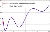
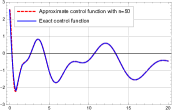
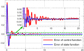
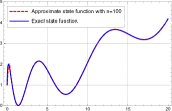
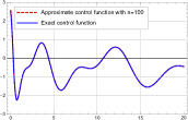
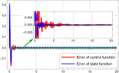
This problem is solved in [11] by approximating the fractional integral by the Grünwald–Letnikov formula (direct GL method), trapezoidal formula (direct TR method), and Simpson formula (direct SI method). A comparison between the results obtained by our method and the aforementioned methods given in [11] is displayed in Table 2. The results show that our method has the same accuracy as the direct SI method. Furthermore, the approximate and exact state and control functions obtained by the present method with n=50𝑛50n=50 and n=100𝑛100n=100, together with the corresponding error functions, are plotted in Figure 1.

Table 1: Example 6.1: error and convergence order for the state and control functions.
x(t)𝑥𝑡x(t) u(t)𝑢𝑡u(t)
n𝑛n En(x)subscript𝐸𝑛𝑥E_{n}(x) ϵn(x)subscriptitalic-ϵ𝑛𝑥\epsilon_{n}(x) En(u)subscript𝐸𝑛𝑢E_{n}(u) ϵn(u)subscriptitalic-ϵ𝑛𝑢\epsilon_{n}(u)
888 1.23e+01.23𝑒01.23e+0 2.342.342.34 3.10e+03.10𝑒03.10e+0 3.633.633.63
161616 2.43e12.43𝑒12.43e-1 3.093.093.09 2.51e12.51𝑒12.51e-1 3.563.563.56
323232 2.86e22.86𝑒22.86e-2 3.413.413.41 2.13e22.13𝑒22.13e-2 2.442.442.44
646464 2.68e32.68𝑒32.68e-3 3.503.503.50 3.92e33.92𝑒33.92e-3 3.373.373.37
128128128 2.36e42.36𝑒42.36e-4 3.523.523.52 3.79e43.79𝑒43.79e-4 3.573.573.57
256256256 2.06e52.06𝑒52.06e-5 3.18e53.18𝑒53.18e-5
Table 2: Example 6.1: comparison of the numerical results obtained by the present method versus methods of [11].
Direct GL method [11] Direct TR method [11] Direct SI method [11] Present method
n𝑛n En(x)subscript𝐸𝑛𝑥E_{n}(x) En(u)subscript𝐸𝑛𝑢E_{n}(u) En(x)subscript𝐸𝑛𝑥E_{n}(x) En(u)subscript𝐸𝑛𝑢E_{n}(u) En(x)subscript𝐸𝑛𝑥E_{n}(x) En(u)subscript𝐸𝑛𝑢E_{n}(u) En(x)subscript𝐸𝑛𝑥E_{n}(x) En(u)subscript𝐸𝑛𝑢E_{n}(u)
100100100 1.11e11.11𝑒11.11e-1 1.68e11.68𝑒11.68e-1 1.48e21.48𝑒21.48e-2 2.07e22.07𝑒22.07e-2 5.60e45.60𝑒45.60e-4 8.99e48.99𝑒48.99e-4 5.63e45.63𝑒45.63e-4 9.03e49.03𝑒49.03e-4
200200200 5.71e25.71𝑒25.71e-2 9.19e29.19𝑒29.19e-2 3.71e33.71𝑒33.71e-3 5.21e35.21𝑒35.21e-3 4.91e54.91𝑒54.91e-5 7.66e57.66𝑒57.66e-5 4.92e54.92𝑒54.92e-5 7.68e57.68𝑒57.68e-5
300300300 3.94e23.94𝑒23.94e-2 6.37e26.37𝑒26.37e-2 1.65e31.65𝑒31.65e-3 2.32e32.32𝑒32.32e-3 1.18e51.18𝑒51.18e-5 1.80e51.80𝑒51.80e-5 1.18e51.18𝑒51.18e-5 1.80e51.80𝑒51.80e-5
Refer to caption
Refer to caption
Refer to caption
Refer to caption
Refer to caption
Refer to caption
Figure 1: Example 6.1: comparison of the exact and numerical solutions along with error functions. Above: n=50𝑛50n=50. Bellow: n=100𝑛100n=100.
Example 6.2.

Consider the following constrained FOCP [19, 20, 21]:

minJ=01(ln2)x(t)𝑑ts.t.Dαx(t)=(ln2)(x(t)+u(t)),x(0)=0,|u(t)|1,x(t)+u(t)2.formulae-sequence𝐽superscriptsubscript012𝑥𝑡differential-d𝑡𝑠𝑡formulae-sequencesuperscript𝐷𝛼𝑥𝑡2𝑥𝑡𝑢𝑡formulae-sequence𝑥00formulae-sequence𝑢𝑡1𝑥𝑡𝑢𝑡2\begin{split}\min~{}&J=\int_{0}^{1}(-\ln 2)x(t)dt\\ s.t.~{}&D^{\alpha}x(t)=(\ln 2)(x(t)+u(t)),\\ &x(0)=0,\\ &\left|u(t)\right|\leq 1,\\ &x(t)+u(t)\leq 2.\end{split} (35)

In this problem, we have tf=1subscript𝑡𝑓1t_{f}=1. By taking n=2𝑛2n=2, the value of hh is given as h=1212h=\frac{1}{2}. We set

Dαx(t)=ATΨ(t),u(t)=UTΨ(t),formulae-sequencesuperscript𝐷𝛼𝑥𝑡superscript𝐴𝑇Ψ𝑡𝑢𝑡superscript𝑈𝑇Ψ𝑡D^{\alpha}x(t)=A^{T}\Psi(t),\quad u(t)=U^{T}\Psi(t), (36)

where

A=[a0,a1,a2]T,U=[u0,u1,u2]T,Ψ(t)=[ψ0(t),ψ1(t),ψ2(t)]T,formulae-sequence𝐴superscriptsubscript𝑎0subscript𝑎1subscript𝑎2𝑇formulae-sequence𝑈superscriptsubscript𝑢0subscript𝑢1subscript𝑢2𝑇Ψ𝑡superscriptsubscript𝜓0𝑡subscript𝜓1𝑡subscript𝜓2𝑡𝑇A=[a_{0},a_{1},a_{2}]^{T},\quad U=[u_{0},u_{1},u_{2}]^{T},\quad\Psi(t)=[\psi_{0}(t),\psi_{1}(t),\psi_{2}(t)]^{T},

with unknown parameters aisubscript𝑎𝑖a_{i}, uisubscript𝑢𝑖u_{i}, i=0,1,2𝑖012i=0,1,2, and

ψ0(t)={2t23t+1,0t1,0,otherwise,subscript𝜓0𝑡cases2superscript𝑡23𝑡10𝑡1missing-subexpressionmissing-subexpression0otherwise\psi_{0}(t)=\left\{\begin{array}[]{ll}2t^{2}-3t+1,&0\leq t\leq 1,\\ &\\ 0,&\text{otherwise},\end{array}\right.
ψ1(t)={4t2+4t,0t1,0,otherwise,subscript𝜓1𝑡cases4superscript𝑡24𝑡0𝑡1missing-subexpressionmissing-subexpression0otherwise\psi_{1}(t)=\left\{\begin{array}[]{ll}-4t^{2}+4t,&0\leq t\leq 1,\\ &\\ 0,&\text{otherwise},\end{array}\right.
ψ2(t)={2t2t,0t1,0,otherwise.subscript𝜓2𝑡cases2superscript𝑡2𝑡0𝑡1missing-subexpressionmissing-subexpression0otherwise\psi_{2}(t)=\left\{\begin{array}[]{ll}2t^{2}-t,&0\leq t\leq 1,\\ &\\ 0,&\text{otherwise}.\end{array}\right.

Taking into account the initial condition in (35), we obtain that

x(t)=ATP(α)Ψ(t),𝑥𝑡superscript𝐴𝑇superscript𝑃𝛼Ψ𝑡x(t)=A^{T}P^{(\alpha)}\Psi(t), (37)

where

P(α)=[0p01p020p11p120p21p22].superscript𝑃𝛼delimited-[]0subscript𝑝01subscript𝑝020subscript𝑝11subscript𝑝120subscript𝑝21subscript𝑝22P^{(\alpha)}=\left[\begin{array}[]{ccc}0&p_{01}&p_{02}\\ 0&p_{11}&p_{12}\\ 0&p_{21}&p_{22}\\ \end{array}\right].

By substituting (37) into the performance index J𝐽J and using (19), we get

J=ln26(4a0p01+a0p02+4a1p11+a1p12+4a2p21+a2p22).𝐽264subscript𝑎0subscript𝑝01subscript𝑎0subscript𝑝024subscript𝑎1subscript𝑝11subscript𝑎1subscript𝑝124subscript𝑎2subscript𝑝21subscript𝑎2subscript𝑝22J=\frac{-\ln 2}{6}\left(4a_{0}p_{01}+a_{0}p_{02}+4a_{1}p_{11}+a_{1}p_{12}+4a_{2}p_{21}+a_{2}p_{22}\right). (38)

Moreover, using (36) and (37), the dynamic system in (35) is reduced to

AT(ln2)(ATP(α)+UT)=0,superscript𝐴𝑇2superscript𝐴𝑇superscript𝑃𝛼superscript𝑈𝑇0A^{T}-(\ln 2)(A^{T}P^{(\alpha)}+U^{T})=0,

which gives the following system of equations:

a0ln2u0=0,a1ln2(a0p01+a1p11+a2p21+u1)=0,a2ln2(a0p02+a1p12+a2p22+u2)=0.formulae-sequencesubscript𝑎02subscript𝑢00formulae-sequencesubscript𝑎12subscript𝑎0subscript𝑝01subscript𝑎1subscript𝑝11subscript𝑎2subscript𝑝21subscript𝑢10subscript𝑎22subscript𝑎0subscript𝑝02subscript𝑎1subscript𝑝12subscript𝑎2subscript𝑝22subscript𝑢20\begin{split}&a_{0}-\ln 2u_{0}=0,\\ &a_{1}-\ln 2\left(a_{0}p_{01}+a_{1}p_{11}+a_{2}p_{21}+u_{1}\right)=0,\\ &a_{2}-\ln 2\left(a_{0}p_{02}+a_{1}p_{12}+a_{2}p_{22}+u_{2}\right)=0.\\ \end{split} (39)

Finally, we take into account the inequality constraints in (35) at τi=i+16subscript𝜏𝑖𝑖16\tau_{i}=\frac{i+1}{6}, i=0,1,,4𝑖014i=0,1,\ldots,4, to obtain

|5u09+5u19u29|1,|2u09+8u19u29|1,|u1|1,|u09+8u19+2u29|1,|u09+5u19+5u29|1,19(5a0p01a0p02+5a1p11a1p12+5a2p21a2p22+5u0+5u1u2)2,19(8a0p01a0p02+8a1p11a1p12+8a2p21a2p22+2u0+8u1u2)2,a0p01+a1p11+a2p21+u12,19(2(4a0p01+a0p02+4a1p11+a1p12+4a2p21+a2p22+4u1+u2)u0)2,19(5(a0p01+a0p02+a1p11+a1p12+a2p21+a2p22+u1+u2)u0)2.formulae-sequence5subscript𝑢095subscript𝑢19subscript𝑢291formulae-sequence2subscript𝑢098subscript𝑢19subscript𝑢291formulae-sequencesubscript𝑢11formulae-sequencesubscript𝑢098subscript𝑢192subscript𝑢291formulae-sequencesubscript𝑢095subscript𝑢195subscript𝑢291formulae-sequence195subscript𝑎0subscript𝑝01subscript𝑎0subscript𝑝025subscript𝑎1subscript𝑝11subscript𝑎1subscript𝑝125subscript𝑎2subscript𝑝21subscript𝑎2subscript𝑝225subscript𝑢05subscript𝑢1subscript𝑢22formulae-sequence198subscript𝑎0subscript𝑝01subscript𝑎0subscript𝑝028subscript𝑎1subscript𝑝11subscript𝑎1subscript𝑝128subscript𝑎2subscript𝑝21subscript𝑎2subscript𝑝222subscript𝑢08subscript𝑢1subscript𝑢22formulae-sequencesubscript𝑎0subscript𝑝01subscript𝑎1subscript𝑝11subscript𝑎2subscript𝑝21subscript𝑢12formulae-sequence1924subscript𝑎0subscript𝑝01subscript𝑎0subscript𝑝024subscript𝑎1subscript𝑝11subscript𝑎1subscript𝑝124subscript𝑎2subscript𝑝21subscript𝑎2subscript𝑝224subscript𝑢1subscript𝑢2subscript𝑢02195subscript𝑎0subscript𝑝01subscript𝑎0subscript𝑝02subscript𝑎1subscript𝑝11subscript𝑎1subscript𝑝12subscript𝑎2subscript𝑝21subscript𝑎2subscript𝑝22subscript𝑢1subscript𝑢2subscript𝑢02\begin{split}&\left|\frac{5u_{0}}{9}+\frac{5u_{1}}{9}-\frac{u_{2}}{9}\right|\leq 1,\\ &\left|\frac{2u_{0}}{9}+\frac{8u_{1}}{9}-\frac{u_{2}}{9}\right|\leq 1,\\ &\left|u_{1}\right|\leq 1,\\ &\left|-\frac{u_{0}}{9}+\frac{8u_{1}}{9}+\frac{2u_{2}}{9}\right|\leq 1,\\ &\left|-\frac{u_{0}}{9}+\frac{5u_{1}}{9}+\frac{5u_{2}}{9}\right|\leq 1,\\ &\frac{1}{9}\left(5a_{0}p_{01}-a_{0}p_{02}+5a_{1}p_{11}-a_{1}p_{12}+5a_{2}p_{21}-a_{2}p_{22}+5u_{0}+5u_{1}-u_{2}\right)\leq 2,\\ &\frac{1}{9}\left(8a_{0}p_{01}-a_{0}p_{02}+8a_{1}p_{11}-a_{1}p_{12}+8a_{2}p_{21}-a_{2}p_{22}+2u_{0}+8u_{1}-u_{2}\right)\leq 2,\\ &a_{0}p_{01}+a_{1}p_{11}+a_{2}p_{21}+u_{1}\leq 2,\\ &\frac{1}{9}\left(2\left(4a_{0}p_{01}+a_{0}p_{02}+4a_{1}p_{11}+a_{1}p_{12}+4a_{2}p_{21}+a_{2}p_{22}+4u_{1}+u_{2}\right)-u_{0}\right)\leq 2,\\ &\frac{1}{9}\left(5\left(a_{0}p_{01}+a_{0}p_{02}+a_{1}p_{11}+a_{1}p_{12}+a_{2}p_{21}+a_{2}p_{22}+u_{1}+u_{2}\right)-u_{0}\right)\leq 2.\end{split} (40)

In summary, the problem is reduced to the minimization of (38) subject to the conditions given in (39) and (40).

In the particular case when α=1𝛼1\alpha=1, the exact solution of the problem is given by

x(t)=2t1,u(t)=1,formulae-sequence𝑥𝑡superscript2𝑡1𝑢𝑡1x(t)=2^{t}-1,\quad u(t)=1,

and the optimal value of the performance index with seven significant digits is J=0.3068528𝐽0.3068528J=-0.3068528. By considering α=1𝛼1\alpha=1, the operational matrix of integration is given by

P(1)=[05241601323012416].superscript𝑃1delimited-[]052416missing-subexpressionmissing-subexpressionmissing-subexpression01323missing-subexpressionmissing-subexpressionmissing-subexpression012416P^{(1)}=\left[\begin{array}[]{ccc}0&\frac{5}{24}&\frac{1}{6}\\ &&\\ 0&\frac{1}{3}&\frac{2}{3}\\ &&\\ 0&-\frac{1}{24}&\frac{1}{6}\\ \end{array}\right].

Therefore, by substituting the elements of P(1)superscript𝑃1P^{(1)} into (38)–(40), the following linear programming problem is produced:

min\displaystyle\min~{} ln26(a0+2a1),26subscript𝑎02subscript𝑎1\displaystyle\frac{-\ln 2}{6}\left(a_{0}+2a_{1}\right),
s.t.formulae-sequence𝑠𝑡\displaystyle s.t.~{} a0u0ln2=0,subscript𝑎0subscript𝑢020\displaystyle a_{0}-u_{0}\ln 2=0,
a1ln2(5a024+a13a224+u1)=0,subscript𝑎125subscript𝑎024subscript𝑎13subscript𝑎224subscript𝑢10\displaystyle a_{1}-\ln 2\left(\frac{5a_{0}}{24}+\frac{a_{1}}{3}-\frac{a_{2}}{24}+u_{1}\right)=0,
a2ln2(a06+2a13+a26+u2)=0,subscript𝑎22subscript𝑎062subscript𝑎13subscript𝑎26subscript𝑢20\displaystyle a_{2}-\ln 2\left(\frac{a_{0}}{6}+\frac{2a_{1}}{3}+\frac{a_{2}}{6}+u_{2}\right)=0,
|5u09+5u19u29|1,5subscript𝑢095subscript𝑢19subscript𝑢291\displaystyle\left|\frac{5u_{0}}{9}+\frac{5u_{1}}{9}-\frac{u_{2}}{9}\right|\leq 1,
|2u09+8u19u29|1,2subscript𝑢098subscript𝑢19subscript𝑢291\displaystyle\left|\frac{2u_{0}}{9}+\frac{8u_{1}}{9}-\frac{u_{2}}{9}\right|\leq 1,
|u1|1,subscript𝑢11\displaystyle\left|u_{1}\right|\leq 1,
|u09+8u19+2u29|1,subscript𝑢098subscript𝑢192subscript𝑢291\displaystyle\left|-\frac{u_{0}}{9}+\frac{8u_{1}}{9}+\frac{2u_{2}}{9}\right|\leq 1,
|u09+5u19+5u29|1,subscript𝑢095subscript𝑢195subscript𝑢291\displaystyle\left|-\frac{u_{0}}{9}+\frac{5u_{1}}{9}+\frac{5u_{2}}{9}\right|\leq 1,
172(7a0+8a13a2+40u0+40u18u2)2,1727subscript𝑎08subscript𝑎13subscript𝑎240subscript𝑢040subscript𝑢18subscript𝑢22\displaystyle\frac{1}{72}\left(7a_{0}+8a_{1}-3a_{2}+40u_{0}+40u_{1}-8u_{2}\right)\leq 2,
118(3a0+4a1a2+4u0+16u12u2)2,1183subscript𝑎04subscript𝑎1subscript𝑎24subscript𝑢016subscript𝑢12subscript𝑢22\displaystyle\frac{1}{18}\left(3a_{0}+4a_{1}-a_{2}+4u_{0}+16u_{1}-2u_{2}\right)\leq 2,
124(5a0+8a1a2+24u1)2,1245subscript𝑎08subscript𝑎1subscript𝑎224subscript𝑢12\displaystyle\frac{1}{24}\left(5a_{0}+8a_{1}-a_{2}+24u_{1}\right)\leq 2,
19(2a0+4a1u0+8u1+2u2)2,192subscript𝑎04subscript𝑎1subscript𝑢08subscript𝑢12subscript𝑢22\displaystyle\frac{1}{9}\left(2a_{0}+4a_{1}-u_{0}+8u_{1}+2u_{2}\right)\leq 2,
172(15a0+40a1+5a28u0+40u1+40u2)2.17215subscript𝑎040subscript𝑎15subscript𝑎28subscript𝑢040subscript𝑢140subscript𝑢22\displaystyle\frac{1}{72}\left(15a_{0}+40a_{1}+5a_{2}-8u_{0}+40u_{1}+40u_{2}\right)\leq 2.

By solving this problem, we find

a0=0.6931472,a1=0.9795332,a2=1.3859775,u0=u1=u2=1.formulae-sequencesubscript𝑎00.6931472formulae-sequencesubscript𝑎10.9795332formulae-sequencesubscript𝑎21.3859775subscript𝑢0subscript𝑢1subscript𝑢21a_{0}=0.6931472,~{}a_{1}=0.9795332,~{}a_{2}=1.3859775,u_{0}=u_{1}=u_{2}=1.

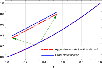
Substituting ui=1subscript𝑢𝑖1u_{i}=1, i=0,1,2𝑖012i=0,1,2, into (36), the exact control function is obtained. The approximate and exact state functions are plotted in Figure 2. In this case, the approximate value of the performance index is J2=0.3063957subscript𝐽20.3063957J_{2}=-0.3063957.

We have employed our method for solving problem (35) with different values of n𝑛n. For all the considered values of n𝑛n, the method gives the exact control function. Table 3 displays the numerical results for x(t)𝑥𝑡x(t), ϵn(x)subscriptitalic-ϵ𝑛𝑥\epsilon_{n}(x), J𝐽J, and the CPU time consumed for solving the resulting linear programming problem. It is seen that the present method gives the exact solution of J𝐽J, with seven significant digits, with n=32𝑛32n=32 and that the convergence order of the state function is O(h4)𝑂superscript4O(h^{4}). In Table 3, the method of [21] refers to the hybrid block-pulse and Taylor polynomials method, the method of [20] denotes the method of hybrid block-pulse and Bernoulli polynomials, and the method of [19] refers to the Bernstein polynomials method.
Refer to caption
Figure 2: Example 6.2: comparison of the exact and numerical state functions with n=2𝑛2n=2 and α=1𝛼1\alpha=1.
Table 3: Numerical results for Example 6.2.
Methods En(x)subscript𝐸𝑛𝑥E_{n}(x) ϵn(x)subscriptitalic-ϵ𝑛𝑥\epsilon_{n}(x) J𝐽J CPU Time
Present n=2𝑛2n=2 8.07e48.07𝑒48.07e-4 4.024.024.02 0.30639570.3063957-0.3063957 0.0150.0150.015
method n=4𝑛4n=4 4.99e54.99𝑒54.99e-5 4.014.014.01 0.30682480.3068248-0.3068248 0.0150.0150.015
n=8𝑛8n=8 3.09e63.09𝑒63.09e-6 4.014.014.01 0.30685110.3068511-0.3068511 0.0150.0150.015
n=16𝑛16n=16 1.92e71.92𝑒71.92e-7 4.004.004.00 0.30685270.3068527-0.3068527 0.0320.0320.032
n=32𝑛32n=32 1.20e81.20𝑒81.20e-8 0.30685280.3068528-0.3068528 0.0320.0320.032
Method of [21] M=3,𝑀3M=3, N=1𝑁1N=1 0.306830.30683-0.30683 40.09140.09140.091
Method of [20] M=3,𝑀3M=3, N=1𝑁1N=1 0.306840.30684-0.30684 53.13353.13353.133
Method of [19] M=3𝑀3M=3 0.306850.30685-0.30685
Example 6.3.

Let us now consider the following nonlinear FOCP [22, 23]:

minJ=01[et(x(t)t4+t1)2+(1+t2)(u(t)+1t+t48000t211077Γ(110))2]𝑑t,s.t.D1.9x(t)=x(t)+u(t),x(0)=1,x(0)=1.\begin{split}\min~{}&J=\int_{0}^{1}\left[e^{t}\left(x(t)-t^{4}+t-1\right)^{2}+(1+t^{2})\left(u(t)+1-t+t^{4}-\frac{8000t^{\frac{21}{10}}}{77\Gamma(\frac{1}{10})}\right)^{2}\right]dt,\\ s.t.~{}&D^{1.9}x(t)=x(t)+u(t),\\ &x(0)=1,\quad x^{\prime}(0)=-1.\end{split}

The state and control functions that minimize the performance index J𝐽J are given by

x(t)=1t+t4,u(t)=1+tt4+800077Γ(110)t2110,formulae-sequence𝑥𝑡1𝑡superscript𝑡4𝑢𝑡1𝑡superscript𝑡4800077Γ110superscript𝑡2110\begin{split}&x(t)=1-t+t^{4},\\ &u(t)=-1+t-t^{4}+\frac{8000}{77\Gamma(\frac{1}{10})}t^{\frac{21}{10}},\end{split}

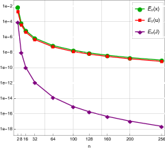
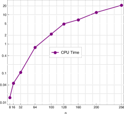
with optimal value Jopt=0subscript𝐽𝑜𝑝𝑡0J_{opt}=0. By applying our method with different values of n𝑛n, we obtain the numerical results displayed in Table 4. In this table, we give a comparison between the results for J𝐽J and CPU times consumed for solving the final algebraic system resulted by our method, the method of [22], which uses Legendre polynomials as the basis functions and the Gauss quadrature rule for integrating the FOCP, and also the method of [23], which employs Bernoulli polynomials and the Gauss quadrature rule for integrating the FOCP. In [22] and [23], m𝑚m refers to the maximum order of the Legendre and Bernoulli polynomials, respectively, that have been used for approximating the state and control functions. It can be seen from Table 4 that the method we suggest here approximates the state and control functions with convergence of order O(h3)𝑂superscript3O(h^{3}). In Figure 3 (left), the results for En(x)subscript𝐸𝑛𝑥E_{n}(x), En(u)subscript𝐸𝑛𝑢E_{n}(u), and En(J)=|JoptJn|subscript𝐸𝑛𝐽subscript𝐽𝑜𝑝𝑡subscript𝐽𝑛E_{n}(J)=|J_{opt}-J_{n}|, obtained by employing our method for some selected values of n𝑛n, are plotted in a logarithmic scale. This figure confirms the O(h3)𝑂superscript3O(h^{3}) accuracy order of the state and control functions. It also shows that the accuracy order of the performance index is higher than O(h3)𝑂superscript3O(h^{3}). Moreover, the CPU times of the method are plotted in Figure 3 (right).

Table 4: Numerical results for Example 6.3.
Methods En(x)subscript𝐸𝑛𝑥E_{n}(x) ϵn(x)subscriptitalic-ϵ𝑛𝑥\epsilon_{n}(x) En(u)subscript𝐸𝑛𝑢E_{n}(u) ϵn(u)subscriptitalic-ϵ𝑛𝑢\epsilon_{n}(u) J𝐽J CPU Time
Present n=4𝑛4n=4 7.10e47.10𝑒47.10e-4 3.393.393.39 2.98e42.98𝑒42.98e-4 3.033.033.03 9.64314e79.64314𝑒79.64314e-7 0.0000.0000.000
method n=8𝑛8n=8 6.75e56.75𝑒56.75e-5 3.333.333.33 3.65e53.65𝑒53.65e-5 3.153.153.15 1.00418e81.00418𝑒81.00418e-8 0.0150.0150.015
n=16𝑛16n=16 6.69e66.69𝑒66.69e-6 3.283.283.28 4.10e64.10𝑒64.10e-6 3.183.183.18 1.06677e101.06677𝑒101.06677e-10 0.0460.0460.046
n=32𝑛32n=32 6.91e76.91𝑒76.91e-7 3.223.223.22 4.52e74.52𝑒74.52e-7 3.173.173.17 1.19487e121.19487𝑒121.19487e-12 0.1090.1090.109
n=64𝑛64n=64 7.42e87.42𝑒87.42e-8 3.183.183.18 5.03e85.03𝑒85.03e-8 3.153.153.15 1.41601e141.41601𝑒141.41601e-14 0.7650.7650.765
n=128𝑛128n=128 8.20e98.20𝑒98.20e-9 3.153.153.15 5.66e95.66𝑒95.66e-9 3.143.143.14 1.75827e161.75827𝑒161.75827e-16 4.9224.9224.922
n=256𝑛256n=256 9.24e109.24𝑒109.24e-10 6.44e106.44𝑒106.44e-10 2.25012e182.25012𝑒182.25012e-18 21.28221.28221.282
Method of [22] m=4𝑚4m=4 5.42028e75.42028𝑒75.42028e-7 0.1410.1410.141
m=8𝑚8m=8 8.22283e108.22283𝑒108.22283e-10 0.2960.2960.296
Method of [23] m=4𝑚4m=4 5.16864e75.16864𝑒75.16864e-7 0.0780.0780.078
m=8𝑚8m=8 4.23025e114.23025𝑒114.23025e-11 0.1710.1710.171
Refer to caption
Refer to caption
Figure 3: Numerical results of Example 6.3 for some selected n𝑛n: the measured En(x)subscript𝐸𝑛𝑥E_{n}(x), En(u)subscript𝐸𝑛𝑢E_{n}(u), and En(J)subscript𝐸𝑛𝐽E_{n}(J) in logarithmic scale (left); CPU time (right)

7 Conclusion

We introduced a new numerical approach for solving fractional optimal control problems (FOCPs). Our scheme uses modified hat functions as basis functions and gives approximations of the control and state variables as linear combinations of such basis functions. The properties of the basis functions, together with those of the Caputo derivative and Riemann–Liouville integral, allow us to reduce the FOCP to a system of nonlinear algebraic equations, which greatly simplifies the problem. An error estimate of the method is proved. Moreover, a generalization is given for solving constrained FOCPs. The method is employed for solving three illustrative examples and the obtained results confirm the efficiency, accuracy, and high performance of our technique when compared with state of the art numerical schemes available in the literature. We claim that our method can be very useful in real applications. We are currently investigating its application to human respiratory syncytial virus infection and to the model introduced in [14]. Another direction of future research consists to generalize our method to variable-order FOCPs, which is an area under development [6, 24].

Acknowledgments

Lima acknowledges support from Fundação para a Ciência e a Tecnologia (FCT, the Portuguese Foundation for Science and Technology) through project UID/MAT/04621/2019; Torres was supported by FCT within project UID/MAT/04106/2019 (CIDMA). The authors are grateful to an anonymous reviewer for suggestions to improve the article.

References

References

  • [1] D. P. Bertsekas, Dynamic programming and optimal control. Vol. I, fourth edition, Athena Scientific, Belmont, MA, 2017.
  • [2] A. S. Leong, D. E. Quevedo and S. Dey, Optimal control of energy resources for state estimation over wireless channels, SpringerBriefs in Electrical and Computer Engineering, Springer, Cham, 2018.
  • [3] R. Almeida and D. F. M. Torres, A survey on fractional variational calculus. In: A. Kochubei, Y. Luchko (Eds.), Handbook of Fractional Calculus with Applications. Vol 1: Basic Theory, De Gruyter, Berlin, Boston, 2019, 347–360. arXiv:1806.05092
  • [4] T. Odzijewicz and D. F. M. Torres, The generalized fractional calculus of variations, Southeast Asian Bull. Math. 38 (2014), no. 1, 93–117. arXiv:1401.7291
  • [5] R. Almeida, S. Pooseh and D. F. M. Torres, Computational methods in the fractional calculus of variations, Imperial College Press, London, 2015.
  • [6] R. Almeida, D. Tavares and D. F. M. Torres, The variable-order fractional calculus of variations, SpringerBriefs in Applied Sciences and Technology, Springer, Cham, 2019. arXiv:1805.00720
  • [7] A. Razminia, M. Asadizadehshiraz and D. F. M. Torres, Fractional order version of the Hamilton–Jacobi–Bellman equation, J. Comput. Nonlinear Dynam. 14 (2019), no. 1, 011005-1–011005-6. arXiv:1810.12882
  • [8] H. Hassani, J. A. Tenreiro Machado and E. Naraghirad, Generalized shifted Chebyshev polynomials for fractional optimal control problems, Commun. Nonlinear Sci. Numer. Simul. 75 (2019), 50–61.
  • [9] M. A. Zaky and J. A. T. Machado, On the formulation and numerical simulation of distributed-order fractional optimal control problems, Commun. Nonlinear Sci. Numer. Simul. 52 (2017), 177–189.
  • [10] M. S. Ali, M. Shamsi, H. Khosravian-Arab, D. F. M. Torres and F. Bozorgnia, A space–time pseudospectral discretization method for solving diffusion optimal control problems with two-sided fractional derivatives, J. Vib. Control 25 (2019), no. 5, 1080–1095. arXiv:1810.05876
  • [11] A. B. Salati, M. Shamsi and D. F. M. Torres, Direct transcription methods based on fractional integral approximation formulas for solving nonlinear fractional optimal control problems, Commun. Nonlinear Sci. Numer. Simul. 67 (2019), 334–350. arXiv:1805.06537
  • [12] W. Li, S. Wang and V. Rehbock, Numerical solution of fractional optimal control, J. Optim. Theory Appl. 180 (2019), no. 2, 556–573.
  • [13] S. Rosa and D. F. M. Torres, Optimal control and sensitivity analysis of a fractional order TB model, Stat. Optim. Inf. Comput. 7 (2019), no. 2, in press. arXiv:1812.04507
  • [14] S. Rosa and D. F. M. Torres, Optimal control of a fractional order epidemic model with application to human respiratory syncytial virus infection, Chaos Solitons Fractals 117 (2018), 142–149. arXiv:1810.06900
  • [15] S. Nemati and P. M. Lima, Numerical solution of nonlinear fractional integro-differential equations with weakly singular kernels via a modification of hat functions, Appl. Math. Comput. 327 (2018), 79–92.
  • [16] S. Nemati, P. Lima and S. Sedaghat, An effective numerical method for solving fractional pantograph differential equations using modification of hat functions, Appl. Numer. Math. 131 (2018), 174–189.
  • [17] I. Podlubny, Fractional differential equations, Mathematics in Science and Engineering, 198, Academic Press, Inc., San Diego, CA, 1999.
  • [18] R. L. Burden, J. D. Faires, Numerical analysis, 9th Edition, Brooks/Cole, Cengage Learning, 2011.
  • [19] M. Alipour, D. Rostamy and D. Baleanu, Solving multi-dimensional fractional optimal control problems with inequality constraint by Bernstein polynomials operational matrices, J. Vib. Control 19 (2013), no. 16, 2523–2540.
  • [20] S. Mashayekhi and M. Razzaghi, An approximate method for solving fractional optimal control problems by hybrid functions, J. Vib. Control 24 (2018), no. 9, 1621–1631.
  • [21] W. Yonthanthum, A. Rattana and M. Razzaghi, An approximate method for solving fractional optimal control problems by the hybrid of block-pulse functions and Taylor polynomials, Optimal Control Appl. Methods 39 (2018), no. 2, 873–887.
  • [22] A. Lotfi, S. A. Yousefi and M. Dehghan, Numerical solution of a class of fractional optimal control problems via the Legendre orthonormal basis combined with the operational matrix and the Gauss quadrature rule, J. Comput. Appl. Math. 250 (2013), 143–160.
  • [23] E. Keshavarz, Y. Ordokhani and M. Razzaghi, A numerical solution for fractional optimal control problems via Bernoulli polynomials, J. Vib. Control 22 (2016), no. 18, 3889–3903.
  • [24] M. D. Ortigueira, D. Valério and J. T. Machado, Variable order fractional systems, Commun. Nonlinear Sci. Numer. Simul. 71 (2019), 231–243.