Yang-Baxter random fields and stochastic vertex models

Abstract.

Bijectivization refines the Yang-Baxter equation into a pair of local Markov moves which randomly update the configuration of the vertex model. Employing this approach, we introduce new Yang-Baxter random fields of Young diagrams based on spin $q$-Whittaker and spin Hall-Littlewood symmetric functions. We match certain scalar Markovian marginals of these fields with (1) the stochastic six vertex model; (2) the stochastic higher spin six vertex model; and (3) a new vertex model with pushing which generalizes the $q$-Hahn PushTASEP introduced recently in [CMP18]. Our matchings include models with two-sided stationary initial data, and we obtain Fredholm determinantal expressions for the $q$-Laplace transforms of the height functions of all these models. Moreover, we also discover difference operators acting diagonally on spin $q$-Whittaker or (stable) spin Hall-Littlewood symmetric functions.

1. Introduction

1.1. Overview

The interplay between symmetric functions and probability blossomed in the last twenty years. In particular, the frameworks of Schur processes [Oko01], [OR03] and Macdonald processes [BC14] has lead to a significant progress in understanding a number of interesting stochastic models from the so-called Kardar-Parisi-Zhang universality class. More recently much attention was directed at the role of quantum integrability (in the form of the Yang-Baxter equation / Bethe ansatz) in the theory of symmetric functions, with further applications to probability. It was discovered that combinatorial properties (most prominently, the Cauchy identity and symmetrization formulas) of many interesting families of symmetric functions can be traced back to integrability (e.g., see [Bor17], [WZJ16]). Employing this point of view and starting with more general solutions to Yang-Baxter equation, [Bor17] and [BW17] defined two families of symmetric functions: the spin Hall-Littlewood (sHL) rational symmetric functions and the spin $q$-Whittaker (sqW) symmetric polynomials, which are one-parameter generalizations, respectively, of the classical Hall-Littlewood and $q$-Whittaker symmetric functions, and obey similar combinatorial relations. See Figure 1 for the scheme of various symmetric functions and degenerations between them.

The goal of the present paper is to further study structural properties of the sHL and sqW functions and connect them to known and new stochastic models. Here is a summary of our results.

• Up to now, it was not clear whether new symmetric functions coming from integrability are eigenfunctions of some difference operators acting on their variables. The presence of such operators is both a key structural feature of the theory of Macdonald polynomials, and an extremely useful tool for applications in probability. We present difference operators acting diagonally on the sHL functions and on the sqW functions which can be used to extract observables ($q$-moments of the first row / column) of the corresponding measures.

• Based on Cauchy identities for sHL / sqW functions, we construct Yang-Baxter fields of random Young diagrams associated with these functions. This allows to relate known stochastic vertex models (stochastic six vertex model [BCG16], stochastic higher spin vertex model [CP16], [BP18]) to sHL and sqW functions. In more detail, we match the (joint) distribution of the height function in each of these vertex models and (joint) distribution of the lengths of the first row / column of Young diagrams from the corresponding random field. The (joint) distribution of the full diagrams is expressed through the (skew) sHL / sqW functions in the same manner as in a Schur / Macdonald process.

• A novel feature of this matching is that we cover a more general class of two-sided stationary initial conditions in stochastic vertex models. These initial conditions depend on two extra parameters (one can think that they encode the particle densities on the left and on the right), and include the step as well as the stationary translation invariant ones (the latter form a one-parameter subfamily).

• We define a new integrable stochastic vertex model with vertex weights expressed through the terminating $q$-hypergeometric series ${}_{4}\phi_{3}$. These weights come from the R matrix entering the Yang-Baxter equation for the sqW functions. The ${}_{4}\phi_{3}$ model generalizes the $q$-Hahn PushTASEP recently introduced in [CMP18].

• For the three stochastic vertex models mentioned above, with the general two-sided stationary initial data, we produce Fredholm determinantal expressions for the $q$-Laplace transform of the height function at a single point.

Let us now describe our results in more detail.

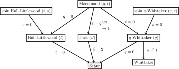
Figure 1. An hierarchy of symmetric functions satisfying Cauchy type summation identities which can be utilized to define random fields of Young diagrams. Arrows mean degenerations. Throughout the introduction and most of the text it is convenient to replace the parameter $t$ by $q$ in spin Hall-Littlewood functions.

1.2. Difference operators

The sHL functions $\mathsf{F}_{\lambda}(u_{1},\dots,u_{n})$ are rational functions of $n$ variables parametrized by Young diagrams $\lambda=\lambda_{1}\geq\lambda_{2}\geq\dots\geq\lambda_{\ell(\lambda)}>0$, $\lambda_{i}\in\mathbb{Z}$. They can be defined by the following formula:

$$\mathsf{F}_{\lambda}(u_{1},\dots,u_{n}):=\frac{(1-q)^{n}}{(q;q)_{n-\ell(\lambda)}}\sum_{\sigma\in\mathfrak{S}_{n}}\sigma\biggl{\{}\prod_{1\leq i<j\leq n}\frac{u_{i}-qu_{j}}{u_{i}-u_{j}}\prod_{i=1}^{n}\left(\frac{u_{i}-s}{1-su_{i}}\right)^{\lambda_{i}}\,\prod_{i=1}^{\ell(\lambda)}\frac{u_{i}}{u_{i}-s}\biggr{\}},$$

where $(q;q)_{n-\ell(\lambda)}$ is the $q$-Pochhammer symbol (cf. Section 1.5), $\mathfrak{S}_{n}$ is the permutation group of $n$ elements, and $\sigma$ acts on the indices of the variables $u_{i}$, but not $\lambda_{i}$ (if $i>\ell(\lambda)$ we have $\lambda_{i}=0$, by agreement). These functions depend on two parameters $q$ and $s$. The functions $\mathsf{F}_{\lambda}(u_{1},\dots,u_{n})$, up to a certain modification, were introduced in [Bor17]; the modification first appeared in [GGW17]. In case $s=0$ these functions become standard Hall-Littlewood functions [Mac95, Chapter III], and for general $s$ many of their properties are very similar to the ones of the standard Hall-Littlewood functions (in particular, Cauchy identity, symmetrization formula, interpretation as a partition function of suitably weighted semistandard Young tableaux).

However, some important properties were missing; perhaps, the most important one is the presence of difference operators acting diagonally on $\mathsf{F}_{\lambda}(u_{1},\dots,u_{n})$. We prove that such operators exist. Define the (Hall-Littlewood versions of) the Macdonald operators by

$$\mathop{\mathfrak{D}_{r}}:=\sum_{\begin{subarray}{c}I\subset\{1,\dots,n\}\\ |I|=r\end{subarray}}\biggl{(}\prod_{\begin{subarray}{c}i\in I\\ j\in\{1,\dots,n\}\setminus I\end{subarray}}\frac{qu_{i}-u_{j}}{u_{i}-u_{j}}\biggr{)}\,T_{0,I},\qquad r=1,2,\ldots,n,$$

where $T_{0,I}$ is the operator setting all $u_{i}$, $i\in I$, to zero. Note that the operators $\mathop{\mathfrak{D}_{r}}$ do not depend on $s$ and coincide with the standard Macdonald operators. We prove the following result.

Theorem 1.1 (Theorem 8.2 in the text).

For all Young diagrams $\lambda$ and $n\in\mathbb{Z}_{\geq 1}$ we have

$$\mathop{\mathfrak{D}_{r}}\mathsf{F}_{\lambda}(u_{1},\ldots,u_{n})=e_{r}(1,q,\dots,q^{n-\ell(\lambda)-1})\,\mathsf{F}_{\lambda}(u_{1},\ldots,u_{n}),$$

where $e_{r}(x_{1},\ldots,x_{k})=\sum_{1\leq i_{1}<\ldots<i_{r}\leq k}x_{i_{1}}\ldots x_{i_{r}}$ is the $r$-th elementary symmetric polynomial.

Let us now turn to the sqW functions $\mathbb{F}^{*}_{\lambda}(\xi_{1},\dots,\xi_{m})$. The shortest way to define them is via the Cauchy identity

$$\sum_{\lambda}\mathbb{F}^{*}_{\lambda}(\xi_{1},\dots,\xi_{m})\,\mathsf{F}_{\lambda^{\prime}}(u_{1},\dots,u_{n})=\prod_{i=1}^{m}\prod_{j=1}^{n}\frac{1+\xi_{i}u_{j}}{1-u_{j}s},$$ (1.1)

where $\lambda^{\prime}$ stands for the conjugation of a Young diagram. (Note that the left-hand side of (1.1) depends on an additional quantization parameter $q$ which enters both $\mathbb{F}^{*}_{\lambda}$ and $\mathsf{F}_{\lambda^{\prime}}$.) This is indeed a definition of the $\mathbb{F}^{*}_{\lambda}$’s, as they can be extracted as coefficients of the expansion thanks to the orthogonality relation for the sHL functions [BCPS15] (which we recall in Proposition 8.6). When $s=0$, $\mathbb{F}^{*}_{\lambda}$ becomes the usual $q$-Whittaker polynomial (i.e., Macdonald polynomial [Mac95, Chapter VI] with $t=0$).

The functions $\mathbb{F}^{*}_{\lambda}(\xi_{1},\dots,\xi_{m})$ were in introduced in [BW17]. They showed that for general $s$ the family $\{\mathbb{F}^{*}_{\lambda}(\xi_{1},\dots,\xi_{m})\}_{\lambda}$ satisfies natural properties (Cauchy identities and representations as partition functions). The question about the existence of difference operators acting diagonally on $\mathbb{F}_{\lambda}^{*}$ was open. We obtain one such difference operator. Define the operator acting on rational functions in $(\theta_{1},\ldots,\theta_{l})$ as follows:

$$\mathop{\mathfrak{E}}:=\sum_{j=1}^{l}\left(1+\frac{s}{\theta_{j}}\right)^{l}\biggl{(}\prod_{i\neq j}\frac{\theta_{j}}{\theta_{j}-\theta_{i}}\biggr{)}T_{q^{-1},\theta_{j}}+\frac{(-s)^{l}}{\theta_{1}\cdots\theta_{l}}\,Id.$$

Here $Id$ is the identity operator, and $T_{q^{-1},\theta_{j}}$ acts by multiplying $\theta_{j}$ by $1/q$.

Theorem 1.2 (Theorem 8.7 in the text).

We have $\mathfrak{E}\,\mathbb{F}^{*}_{\lambda}(\theta_{1},\ldots,\theta_{l})=q^{-\lambda_{1}}\mathbb{F}^{*}_{\lambda}(\theta_{1},\ldots,\theta_{l})$ for all Young diagrams $\lambda$ and all $l\in\mathbb{Z}_{\geq 1}$.

Note that in the classical theory, as well as in the case of sHL functions, we have many eigenoperators of all orders, rather than just one. The existence of higher order eigenoperators for the sqW functions remains open. However, already the presence of one operator brings a lot from both algebraic combinatorial and probabilistic points of view. In particular, first row / column observables of measures based on sqW functions can be extracted and analyzed via the already standard technique introduced in [BC14] for Macdonald measures.

Remark 1.3.

We originally arrived at eigenoperators for the sqW and sHL functions through $q$-moments of the stochastic higher spin six vertex model computed before [CP16], [BP18]. Namely, we used the matching via the Yang-Baxter field (see below in Section 1.3) to recognize that these $q$-moments are at the same time $q$-moments of the measures on Young diagrams expressed through the sHL and sqW functions. The difference operators arise by reversing the $q$-moment computations starting from known contour integrals. However, our proofs of the eigenrelations presented in the paper are more direct, and use only the necessary minimum of the properties of the sHL and the sqW functions.

1.3. Yang-Baxter fields and matching to stochastic vertex models

The usefulness of symmetric functions in probabilistic questions is greatly emphasized by the frameworks of Schur and Macdonald processes. This approach stems from the combination of two general ideas. First, asymptotic behavior of random Young diagrams with probabilistic weights coming from a symmetric function summation identity is often accessible via exact computations with symmetric functions. Second, such Young diagrams turn out to be related to many natural probabilistic models. In order to quantify this relation, one needs to utilize certain combinatorial structures behind the symmetric functions.

First examples of such usage involved RSK (Robinson-Schensted-Knuth) correspondence to establish a relation between Schur functions and models of longest increasing subsequences / last passage percolation / TASEP [BDJ99], [Joh00], [O’C03a], [O’C03]. A bit later, a simpler construction not based on RSK was suggested in [BF14]. In the present paper we employ the third type of construction introduced in [BP17] — the Yang-Baxter fields. (A more detailed historical overview of all these constructions is given in Section 2.6.) We construct three Yang-Baxter fields based on three types of Cauchy identities for the sHL and sqW functions. Let us formulate a sample result in detail.

Fix $q\in[0,1)$, $s\in(-1,0)$, and inhomogeneity parameters $\{\theta_{x}\}_{x\in\mathbb{Z}_{\geq 0}}$, $\{u_{y}\}_{y\in\mathbb{Z}_{\geq 0}}$, satisfying $\theta_{x}\in[-s,-s^{-1}]$, $u_{y}\in[0,1)$. Informally, the stochastic higher spin vertex model [CP16], [BP18] is a random collection of paths on edges of $\mathbb{Z}_{\geq 0}\times\mathbb{Z}_{\geq 0}$ such that each vertex $(x,y)$ has one of four possible types from Figure 2 and contributes the weight shown there with $\theta=\theta_{x}$ and $u=u_{y}$. We also need to prescribe (possibly random) boundary conditions $b_{i}^{\mathrm{v}}\in\left\{0,1\right\}$, $b_{j}^{\mathrm{h}}\in\mathbb{Z}_{\geq 0}$, which parametrize the number of arrows coming into the quadrant from the left and from below, respectively.

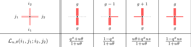
Figure 2. Stochastic vertex weights $\mathcal{L}_{u,\theta}(i_{1},j_{1};i_{2},j_{2})$ for the higher spin model.

In more detail, the stochastic higher spin six vertex model is the (unique) probability measure on the set of up-right directed paths on $\mathbb{Z}_{\geq 0}\times\mathbb{Z}_{\geq 0}$ (with multiple vertical paths allowed per edge, but at most one horizontal path per edge) satisfying:

• Each vertex $(0,y)$ at the vertical boundary $\{(0,y^{\prime}):y^{\prime}\geq 1\}$ emanates a path initially pointing to the right if $b^{\mathrm{v}}_{y}=1$;

• Each vertex $(x,0)$ at the horizontal boundary $\{(x^{\prime},0):x^{\prime}\geq 1\}$ emanates $b^{\mathrm{h}}_{x}$ paths initially pointing upward;

• For each $(x,y)$, conditioned to the path configuration at all vertices $(x^{\prime},y^{\prime})$ such that $x^{\prime}+y^{\prime}<x+y$, the probability of a vertex configuration $(i_{1},j_{1};i_{2},j_{2})$ at $(x,y)$ is given by $\mathcal{L}_{u_{y},\theta_{x}}(i_{1},j_{1};i_{2},j_{2})$. Moreover, the random choices made at diagonally adjacent vertices $\ldots,(x-1,y+1),(x,y),(x+1,y-1),\ldots$ are independent under the same condition.

Take the step boundary conditions $b_{i}^{\mathrm{v}}\equiv 1$, $b_{j}^{\mathrm{h}}\equiv 0$. Let $\mathfrak{h}^{\mathrm{HS}}(x,y)$ be the height function, which is defined as the number of paths which go through or to the right of the point $(x,y)$. We are interested in the distribution of $\mathfrak{h}^{\mathrm{HS}}(x,y)$.

On the symmetric function side, let us consider a random Young diagram $\lambda^{(x,y)}$ with

$$\mathrm{Prob}(\lambda^{(x,y)}=\nu)=\prod_{\begin{subarray}{c}1\leq i\leq x\\ 1\leq j\leq y\end{subarray}}\frac{1-u_{j}s}{1+u_{j}\theta_{i}}\,\mathsf{F}_{\nu}(u_{1},\dots,u_{y})\,\mathbb{F}^{*}_{\nu^{\prime}}(\theta_{1},\dots,\theta_{x}).$$ (1.2)

Cauchy identity (1.1) implies that the sum of the above probabilities over all $\nu$ is equal to 1, as it should be. The next result is a particular case of Theorem 7.18 in the text:

Theorem 1.4.

For any fixed $(x,y)$ in the quadrant, the random variables $y-\ell(\lambda^{(x,y)})$ and $\mathfrak{h}^{\mathrm{HS}}(x+1,y)$ have the same distribution.

Our Theorem 7.18 contains a more general statement. First, it provides a matching of the whole two-dimensional array $\{\mathfrak{h}^{\mathrm{HS}}(x+1,y)\}$ to an array of scalar observables of a Yang-Baxter field of Young diagrams $\{\lambda^{(x,y)}\}$ which we construct. In particular, joint distributions of $\mathfrak{h}^{\mathrm{HS}}(x+1,y)$, when $(x,y)$ follow a down-right path, can be accessed through a suitable analogue of a Schur or Macdonald process. Second, Theorem 7.18 includes more general boundary conditions for the vertex model, at a cost of suitably modifying the symmetric functions in the right-hand side of (1.2). Namely, we allow $b_{i}^{\mathrm{v}}\in\left\{0,1\right\}$ to be independent Bernoulli random variables, and $b_{i}^{\mathrm{h}}\in\mathbb{Z}_{\geq 0}$ to be independent $q$-negative binomial random variables (cf. Section 1.5 for the latter). We call such boundary conditions of the field of Young diagrams (two-sided) scaled geometric, they match with two-sided stationary boundary conditions in stochastic vertex models.

The matching we just described in Theorem 1.4 arises in the setting of the Cauchy identity (1.1) involving one sHL and one sqW function. We consider two other Cauchy identities, one with two sHL functions, and another with two sqW functions. The vertex models and the corresponding matchings are described in Section 7.2 and Section 7.4. In all cases we prove analogues of Theorem 1.4 (and the more general Theorem 7.18). The matchings between stochastic vertex models with two-sided stationary boundary conditions and symmetric functions have not been known before in any of the cases.

In the sHL/sHL case, on the vertex model side we obtain the stochastic six vertex model [GS92], [BCG16] and essentially recover (a new degeneration of) the matching of [BP17]. We observe a curious property that the stochastic six vertex model is independent of the parameter $s$, while this parameter enters the sHL/sHL Yang-Baxter field. This independence of $s$ might be explained by Theorem 1.1: the eigenoperators for the spin Hall-Littlewood polynomials do not depend on $s$ either.

The extension of the sHL/sHL field matching to the stochastic six vertex model to the two-sided stationary boundary conditions is new. In the sqW/sqW situation the Yang-Baxter field produces a new integrable stochastic vertex model with vertex weights expressed through the terminating $q$-hypergeometric series ${}_{4}\phi_{3}$. This model generalises the $q$-Hahn PushTASEP [CMP18]. We match the height function of this model to a field of random Young diagrams whose distributions are expressed through a product of two sqW functions.

1.4. Fredholm determinants for observables

The difference operators $\mathfrak{D}_{1}$ and $\mathfrak{E}$ diagonal in the sHL or sqW functions, respectively, allow to express (in a nested contour integral form) the $q$-moments of the height function in each of the three vertex models with step boundary conditions. It is known (e.g., see [BCS14]) that such $q$-moment formulas can be organized into generating series leading to Fredholm determinantal formulas for the $q$-Laplace transform $\mathbb{E}\left(1/(\zeta q^{\mathcal{H}(x,y)};q)_{\infty}\right)$. where $\mathcal{H}(x,y)$ is the height function in either of the three models. This approach works well both for the stochastic six vertex and stochastic higher spin six vertex models with step boundary conditions.

However, for the ${}_{4}\phi_{3}$ vertex model only finitely many of the $q$-moments exist, and thus the generating series cannot be used. Moreover, for the more general two-sided stationary boundary conditions, explicit $q$-moments are not known and also may not be finite. We overcome both these issues at the same time by considering an analytic continuation based on the fusion procedure for vertex models [KRS81] (see [CP16] for a stochastic interpretation of fusion). We start with the Fredholm determinant for the (inhomogeneous) stochastic six vertex model with parameters $(v_{x},u_{y})$, where $(x,y)\in\mathbb{Z}_{\geq 0}^{2}$. Then we replace each $u_{i}$ and $v_{j}$ by a finite geometric sequence $u_{i},qu_{i},\ldots,q^{J_{i}-1}u_{i}$ and $v_{j},qv_{j},\ldots,q^{I_{j}-1}v_{j}$. It turns out that the resulting measure depends on the parameters $(v_{x},q^{I_{x}},u_{y},q^{J_{y}})$ in an analytic way. Then, taking certain specializations of these parameters, we can get to both the sqW functions and the two-sided stationary boundary conditions in the vertex models. The fusion and analytic continuation from sHL functions to the sqW ones was first performed in [BW17].

The Fredholm determinantal formula we obtain in the sqW/sqW setting in particular establishes the Fredholm determinant for the $q$-Hahn PushTASEP which was conjectured in [CMP18].

Analytic continuations leading to Fredholm determinants for stationary stochastic particle systems were performed in [BCFV15] ($q$-Whittaker measures and random polymers) and [Agg18] (stochastic six vertex model). In the first reference, the continuation significantly used the structure of the algebra of symmetric functions. Our analytic continuation based on fusion is more similar to the approach taken in the second reference, but due to connections with sHL and sqW symmetric functions, the argument is more straightforward.

1.5. Notation

Throughout the paper we use the $q$-Pochhammer symbols

$$(a;q)_{n}=\begin{cases}1,&n=0;\\ \prod_{i=1}^{n}(1-aq^{i-1}),&n\geq 1;\\ \prod_{i=n}^{-1}(1-aq^{i})^{-1},&n\leq-1,\end{cases}\qquad\text{and}\qquad(a;q)_{\infty}=\prod_{i=1}^{\infty}(1-aq^{i-1}).$$ (1.3)

We also use the notation

$$\begin{split}{}_{k+1}\overline{\phi}_{k}\left(\begin{minipage}{76.82234pt} \centering{$q^{-n};a_{1},\dots,a_{k}$}\\ \centering{$b_{1},\dots,b_{k}$} \@add@centering\@add@centering\end{minipage}\Big{|}\,q,z\right)&=\prod_{i=1}^{k}(b_{i};q)_{n}\cdot{}_{k+1}{\phi}_{k}\left(\begin{minipage}{76.82234pt} \centering{$q^{-n};a_{1},\dots,a_{k}$}\\ \centering{$b_{1},\dots,b_{k}$} \@add@centering\@add@centering\end{minipage}\Big{|}\,q,z\right)\\ &=\sum_{j=0}^{n}z^{j}\,\frac{(q^{-n};q)_{j}}{(q;q)_{j}}\prod_{i=1}^{k}(a_{i};q)_{j}(q^{j}b_{i};q)_{n-j}\end{split}$$ (1.4)

for the regularized terminating $q$-hypergeometric series.

We say that a random variable $X$ has the $q$-negative binomial distribution with parameters $(r,p)$, or $X\sim q\textnormal{-}\mathrm{NB}(r,p)$, if

$$\mathrm{Prob}\{X=k\}=p^{k}\frac{(r;q)_{k}}{(q;q)_{k}}\frac{(p;q)_{\infty}}{(pr;q)_{\infty}}.$$ (1.5)

In case $r=0$ we say that $X$ is a $q$-Poisson random variable of parameter $p$, or $X\sim q\textnormal{-}\mathrm{Poi}(p)$ (sometimes this distribution is also called $q$-geometric). Finally, the Bernoulli random variable $X\sim\mathrm{Ber}(p)$, $X\in\left\{0,1\right\}$, has $\mathrm{Prob}\{X=1\}=p$ and $\mathrm{Prob}\{X=0\}=1-p$.

1.6. Outline

In Section 2 we outline a general formalism for constructing random fields from symmetric (rational) functions. In Section 3 we recall the spin Hall-Littlewood and spin $q$-Whittaker symmetric functions introduced in [Bor17] and [BW17], respectively. In Section 4 we consider the general form of the skew Cauchy equation which follows from the fused Yang-Baxter equation, and in Section 5 consider yet another family of its specializations which we refer to as “scaled geometric”. In Section 6 we apply bijectivization to the Yang-Baxter equations obtaining local stochastic moves of Yang-Baxter type. In Section 7 we discuss the Yang-Baxter fields thus arising together with their scalar marginals (projections). In Section 8 we define difference operators acting diagonally on our symmetric functions, and study their properties. In Section 9 we write down Fredholm determinantal observables for stochastic particle systems arising from our Yang-Baxter fields. Finally, in Appendix A we list all instances of the Yang-Baxter equation employed in the paper, and discuss the nonnegativity of terms entering these equations.

Acknowledgments

We are grateful to Alexei Borodin for helpful discussions, and to Ivan Corwin for valuable comments on an earlier version of the text. This work has started when MM and LP participated in the program “Non-equilibrium systems and special functions” at MATRIX Institute, and we are grateful to the organizers for hospitality and support. The work of AB was partially supported by the German Research Foundation under Germany’s Excellence Strategy – EXC 2047 “Hausdorff Center for Mathematics”. LP was partially supported by the NSF grant DMS-1664617.

2. Random fields from skew Cauchy identities

In this section we describe an abstract formalism of random fields which is applied to several concrete situations in the rest of the paper.

2.1. Skew Cauchy structures

The fields we consider in this paper are collections of random Young diagrams indexed by points of the two-dimensional quadrant $\mathbb{Z}_{\geq 0}^{2}$. A Young diagram (= partition) is a sequence of integers $\lambda=(\lambda_{1}\geq\ldots\geq\lambda_{\ell(\lambda)}>0)$. The quantity $\ell(\lambda)$ is called the length of the Young diagram $\lambda$. Denote by $\mathbb{Y}$ the set of all Young diagrams including the empty one $\lambda=\varnothing$ (by agreement, $\ell(\varnothing)=0$). It is convenient to be able to add zeros at the end of a Young diagram $\lambda$, and to not distinguish the sequences $(\lambda_{1},\ldots,\lambda_{\ell})$ and $(\lambda_{1},\ldots,\lambda_{\ell},0)$.

Assume that for every pair of Young diagrams $\lambda,\mu$ and any $k\in\mathbb{Z}_{\geq 1}$ we are given two functions $\mathfrak{F}_{\lambda/\mu}(u_{1},\ldots,u_{k})$ and $\mathfrak{G}_{\lambda/\mu}(u_{1},\ldots,u_{k})$ (which may also depend on some external parameters). This data is called a skew Cauchy structure if the functions satisfy the following properties:

1. The functions are rational in the $u_{i}$’s and are symmetric with respect to permutations of $u_{1},\ldots,u_{k}$.

2. Define relations $\prec_{k}$ and $\mathop{\dot{\prec}_{k}}$ on $\mathbb{Y}\times\mathbb{Y}$ such that

   $$\mathfrak{F}_{\lambda/\mu}(u_{1},\ldots,u_{k})\neq 0\quad\textnormal{iff $\mu\prec_{k}\lambda$};\qquad\mathfrak{G}_{\lambda/\mu}(u_{1},\ldots,u_{k})\neq 0\quad\textnormal{iff $\mu\mathop{\dot{\prec}_{k}}\lambda$}.$$ (2.1)

   Moreover, for each $\lambda$ the sets $\left\{\mu\colon\mu\prec_{k}\lambda\right\}$ and $\left\{\rho\colon\rho\mathop{\dot{\prec}_{k}}\lambda\right\}$ are finite. By agreement, we extend these relations to $k=0$ and set $\mathfrak{F}_{\lambda/\mu}(\varnothing)=\mathfrak{G}_{\lambda/\mu}(\varnothing)=\mathbf{1}_{\lambda=\mu}$.

3. (Branching rules) For each $1\leq m\leq k-1$ we have

   $$\mathfrak{F}_{\lambda/\mu}(u_{1},\ldots,u_{k})=\sum_{\varkappa}\mathfrak{F}_{\lambda/\varkappa}(u_{1},\ldots,u_{m})\mathfrak{F}_{\varkappa/\mu}(u_{m+1},\ldots,u_{k}),$$ (2.2)

   and the same branching rule for $\mathfrak{G}_{\lambda/\mu}$ (obtained by replacing each $\mathfrak{F}$ above by $\mathfrak{G}$) holds, too. Note that the sum over $\varkappa$ above is finite.

4. (Skew Cauchy identity) There exists a rational function $\Pi(u;v)$ and a subset $\mathsf{Adm}\subseteq\mathbb{C}^{2}$ such that for all $(u,v)\in\mathsf{Adm}$ one has (see Figure 3 for the illustration)

   $$\sum_{\nu}\mathfrak{F}_{\nu/\mu}(u)\mathfrak{G}_{\nu/\lambda}(v)=\Pi(u;v)\sum_{\varkappa}\mathfrak{F}_{\lambda/\varkappa}(u)\mathfrak{G}_{\mu/\varkappa}(v).$$ (2.3)

   Note that the sum over $\varkappa$ in the right-hand side is finite while the sum over $\nu$ in the left-hand side might be infinite. The set $\mathsf{Adm}$ corresponds to pairs $(u,v)$ for which the infinite sum converges.

5. (Nonnegativity) There exist two sets $\mathsf{P},\dot{\mathsf{P}}\subseteq\mathbb{C}$ such that

   $$\mathfrak{F}_{\lambda/\mu}(u_{1},\ldots,u_{k})\geq 0,\quad u_{i}\in\mathsf{P}\textnormal{ for all $i$};\qquad\mathfrak{G}_{\lambda/\mu}(v_{1},\ldots,v_{k})\geq 0,\quad v_{j}\in\dot{\mathsf{P}}\textnormal{ for all $j$}.$$

Figure 3. An illustration of relations between the four diagrams $\lambda,\mu,\varkappa$, and $\nu$ in the skew Cauchy identity (2.3). The variable $u$ should be thought of corresponding to the vertical direction, and $v$ corresponds to the horizontal one. Here we are using the shorthand notation $\mathop{\prec}=\mathop{\prec_{1}}$ and $\mathop{\dot{\prec}}=\mathop{\dot{\prec}_{1}}$.

Remark 2.1.

The functions $\mathfrak{F}_{\lambda/\mu}$ and $\mathfrak{G}_{\lambda/\mu}$ are rational thus might be undefined for special values of the variables $u_{i}$ or the external parameters. Therefore, all statements in this section should be understood in the sense of generic variables and parameters (i.e., outside vanishing sets of some algebraic expressions).

The branching rules (2.2) imply that for any $\mu,\lambda$ the function $\mathfrak{F}_{\lambda/\mu}(u_{1},\ldots,u_{k})$ vanishes unless there exists a sequence of Young diagrams $\{\varkappa^{(i)}\}$ with

$$\mu\prec_{1}\varkappa^{(1)}\prec_{1}\varkappa^{(2)}\prec_{1}\ldots\prec_{1}\varkappa^{(k-1)}\prec_{1}\lambda.$$

If $\mathfrak{F}_{\lambda/\mu}(u)\neq 0$ for all pairs $\mu\prec_{1}\lambda$, then we can replace the relation $\prec_{k}$ by the existence of a sequence $\varkappa^{(i)}$ as above, and (2.1) will continue to hold. A similar remark is valid for $\mathop{\dot{\prec}_{k}}$, too.

Note also that the skew Cauchy identity for single variables (2.3) together with (2.2) implies the skew Cauchy identity for any number of variables:

$$\sum_{\nu}\mathfrak{F}_{\nu/\mu}(u_{1},\ldots,u_{n})\mathfrak{G}_{\nu/\lambda}(v_{1},\ldots,v_{m})=\prod_{i=1}^{n}\prod_{j=1}^{m}\Pi(u_{i};v_{j})\sum_{\varkappa}\mathfrak{F}_{\lambda/\varkappa}(u_{1},\ldots,u_{n})\mathfrak{G}_{\mu/\varkappa}(v_{1},\ldots,v_{m}),$$ (2.4)

where $(u_{i},v_{j})\in\mathsf{Adm}$ for all $i,j$.

Example 2.2.

The prototypical example of a skew Cauchy structure is given by the Schur symmetric polynomials [Mac95, Chapter I]:

$$\mathfrak{F}_{\lambda/\mu}(u_{1},\ldots,u_{k})=\mathfrak{G}_{\lambda/\mu}(u_{1},\ldots,u_{k})=s_{\lambda/\mu}(u_{1},\ldots,u_{k}),$$

where $s_{\lambda/\mu}$ is the skew Schur polynomial. The relations $\mu\prec_{1}\lambda$ and $\mu\mathop{\dot{\prec}_{1}}\lambda$ are the same and mean interlacing:

$$\mu\prec\lambda\qquad\Leftrightarrow\qquad\lambda_{1}\geq\mu_{1}\geq\lambda_{2}\geq\mu_{2}\geq\ldots.$$

The factor in the right-hand side of the skew Cauchy identity is $\Pi(u;v)=\dfrac{1}{1-uv}$, and the convergence in the left-hand side holds with $\mathsf{Adm}=\left\{(u,v)\colon|uv|<1\right\}$. The nonnegativity sets are $\mathsf{P}=\dot{\mathsf{P}}=\mathbb{R}_{\geq 0}$, and the fact that $s_{\lambda/\mu}(u_{1},\ldots,u_{k})\geq 0$ for $u_{i}\geq 0$ follows from the combinatorial formula for the skew Schur polynomials representing them as generating functions of semistandard Young tableaux of the skew shape $\lambda/\mu$.

This Schur skew Cauchy structure will serve as a running example throughout this section. In the rest of the paper we consider other skew Cauchy structures associated with spin Hall-Littlewood and spin $q$-Whittaker functions.

2.2. Gibbs measures

Through the branching rules, each family of functions $\mathfrak{F}_{\lambda/\mu}$ and $\mathfrak{G}_{\lambda/\mu}$ leads to a version of a Gibbs property. This property also depends on a choice of parameters $u_{1},u_{2},\ldots\in\mathsf{P}$ or $v_{1},v_{2},\ldots\in\dot{\mathsf{P}}$, respectively, which we assume fixed.

Definition 2.3 (Gibbs measures).

A probability measure on a (finite or infinite) sequence of Young diagrams

$$\lambda^{(0)}\prec_{1}\lambda^{(1)}\prec_{1}\ldots\prec_{1}\lambda^{(n)}\prec_{1}\ldots$$

is called $\mathfrak{F}$-Gibbs (with parameters $u_{i}$) if for all $m,n$ with $0\leq m<n-1$, the conditional distribution of $\lambda^{(m+1)},\ldots,\lambda^{(n-1)}$ given $\tau=\lambda^{(m)}$ and $\rho=\lambda^{(n)}$ has the form

$$\frac{1}{Z}\,\mathfrak{F}_{\lambda^{(m+1)}/\tau}(u_{m+1})\mathfrak{F}_{\lambda^{(m+2)}/\lambda^{(m+1)}}(u_{m+2})\ldots\mathfrak{F}_{\rho/\lambda^{(n-1)}}(u_{n}),$$

and, in particular, is independent of $\lambda^{(i)}$ with $i<m$ or $i>n$. The normalizing constant has the form $Z=\mathfrak{F}_{\rho/\tau}(u_{m+1},\ldots,u_{n})$ by (2.2). Note that the set of sequences $\lambda^{(m)}\prec_{1}\lambda^{(m+1)}\prec_{1}\ldots\prec_{1}\lambda^{(n)}$ with fixed $\lambda^{(m)}$ and $\lambda^{(n)}$ is finite, so there are no convergence issues in defining $Z$.

The $\mathfrak{G}$-Gibbs property is defined in a similar way.

Example 2.4.

In the Schur case with $u_{i}\equiv u$ for all $i$, the Gibbs property reduces to the one with uniform conditional probabilities. That is, a measure on an interlacing sequence of diagrams $\varnothing\prec\lambda^{(1)}\prec\lambda^{(2)}\prec\ldots$ is (uniform) Gibbs if, conditioned on any $\lambda^{(n)}=\rho$, the distribution of $\lambda^{(1)},\ldots,\lambda^{(n-1)}$ is uniform among all sequences of Young diagrams satisfying the interlacing constraints.

2.3. Random fields associated to a skew Cauchy structure

Fix a skew Cauchy structure $(\mathfrak{F},\mathfrak{G})$ and parameters

$$u_{1},u_{2},\ldots;\ v_{1},v_{2},\ldots,\quad\textnormal{such that}\quad\textnormal{$(u_{x},v_{y})\in\mathsf{Adm}$, $u_{x}\in\mathsf{P}$, $v_{y}\in\dot{\mathsf{P}}$ for all $x,y$.}$$ (2.5)

A random field corresponding to this data is a family of random Young diagrams $\boldsymbol{\lambda}=\{\lambda^{(x,y)}\}$ indexed by points of the quadrant $(x,y)\in\mathbb{Z}_{\geq 0}^{2}$ with a certain spatial dependence structure determined by the functions $\mathfrak{F}_{\nu/\mu}$ and $\mathfrak{G}_{\nu/\mu}$. We begin by describing the appropriate class of boundary conditions.

Definition 2.5 (Gibbs boundary conditions).

A random two-sided sequence of Young diagrams

$$\boldsymbol{\tau}=\bigl{(}\ldots\succ_{1}\tau^{(0,3)}\succ_{1}\tau^{(0,2)}\succ_{1}\tau^{(0,1)}\succ_{1}\tau^{(0,0)}\mathop{\dot{\prec}_{1}}\tau^{(1,0)}\mathop{\dot{\prec}_{1}}\tau^{(2,0)}\mathop{\dot{\prec}_{1}}\tau^{(3,0)}\mathop{\dot{\prec}_{1}}\ldots\bigr{)}$$ (2.6)

is called an $(\mathfrak{F},\mathfrak{G})$-Gibbs boundary condition (or a Gibbs boundary condition, for short) if the sequences $\{\tau^{(0,y)}\}_{y\geq 0}$ and $\{\tau^{(x,0)}\}_{x\geq 0}$ are $\mathfrak{F}$-Gibbs and $\mathfrak{G}$-Gibbs, respectively (in the sense of Definition 2.3, with parameters (2.5)), and, moreover, the sequences $\{\tau^{(0,y)}\}_{y\geq 1}$ and $\{\tau^{(x,0)}\}_{x\geq 1}$ are conditionally independent given $\tau^{(0,0)}$.

For a Gibbs boundary condition $\boldsymbol{\tau}$ denote

$$Z^{(x,y)}_{\mathrm{boundary}}:=\sum_{\tau^{(0,0)}}\mathfrak{F}_{\tau^{(0,y)}/\tau^{(0,0)}}(u_{1},\ldots,u_{y})\mathfrak{G}_{\tau^{(x,0)}/\tau^{(0,0)}}(v_{1},\ldots,v_{x}),\qquad(x,y)\in\mathbb{Z}_{\geq 0}^{2}.$$ (2.7)

This quantity is random and depends on $\tau^{(x,0)}$ and $\tau^{(0,y)}$.

We will mostly deal with the following particular case of Gibbs boundary conditions:

Definition 2.6 (Step-type boundary conditions).

A Gibbs boundary condition $\boldsymbol{\tau}$ is called step-type in the vertical (resp., horizontal) direction if the $\mathfrak{F}$-Gibbs distribution of the sequence $\{\tau^{(0,y)}\}_{y\geq 0}$ (resp., the $\mathfrak{G}$-Gibbs distribution of $\{\tau^{(x,0)}\}_{x\geq 0}$) is supported on a single sequence. That is, the boundary diagrams are nonrandom but the Gibbs property still holds.

A step-type boundary condition $\boldsymbol{\tau}$ is the one which is step-type in both horizontal and vertical directions. For such boundary conditions the quantity $Z^{(x,y)}_{\mathrm{boundary}}$ (2.7) is not random and is readily written down (e.g., in some examples $\tau^{(0,y)}=\tau^{(x,0)}=\tau^{(0,0)}=\varnothing$). See Section 2.6 below for the origin of the term “step”.

For $(x,y)\in\mathbb{Z}_{\geq 0}^{2}$ denote the northwest and the southeast quadrants by

$$\mathrm{NW}_{(x,y)}:=\{(m,n)\in\mathbb{Z}_{\geq 0}^{2}\colon m\leq x,\ n\geq y\},\qquad\mathrm{SE}\,_{(x,y)}:=\{(m,n)\in\mathbb{Z}_{\geq 0}^{2}\colon m\geq x,\ n\leq y\}.$$

We are now in a position to formulate the main definition of the section:

Definition 2.7 (Random fields).

A family of random Young diagrams $\boldsymbol{\lambda}=\{\lambda^{(x,y)}\colon(x,y)\in\mathbb{Z}_{\geq 0}^{2}\}$ is called a random field associated with the skew Cauchy structure $(\mathfrak{F},\mathfrak{G})$ and parameters (2.5) with a Gibbs boundary condition $\boldsymbol{\tau}$ if:

1. The diagrams satisfy $\lambda^{(x,y)}\prec_{1}\lambda^{(x,y+1)}$ and $\lambda^{(x,y)}\mathop{\dot{\prec}}_{1}\lambda^{(x+1,y)}$ for all $(x,y)\in\mathbb{Z}_{\geq 0}^{2}$.

2. The diagrams at the boundary of the quadrant $\mathbb{Z}_{\geq 0}^{2}$ agree with $\boldsymbol{\tau}$: $\lambda^{(x,0)}=\tau^{(x,0)}$, $\lambda^{(0,y)}=\tau^{(0,y)}$ for all $x,y\geq 0$.

3. For all $(x,y)\in\mathbb{Z}_{\geq 0}^{2}$, let us use the shorthand notation

   $$\varkappa=\lambda^{(x,y)},\qquad\mu=\lambda^{(x+1,y)},\qquad\lambda=\lambda^{(x,y+1)},\qquad\nu=\lambda^{(x+1,y+1)}$$ (2.8)

   (which matches Figure 3). We require that

   $$\begin{split}\mathop{\mathrm{Prob}}\bigl{(}\varkappa\mid\lambda^{(m,n)}\colon(m,n)\in\mathrm{NW}_{(x,y+1)}\cup\mathrm{SE}\,_{(x+1,y)}\bigr{)}&=\mathop{\mathrm{Prob}}\left(\varkappa\mid\lambda,\mu\right)=\frac{\mathfrak{F}_{\lambda/\varkappa}(u_{y+1})\mathfrak{G}_{\mu/\varkappa}(v_{x+1})}{Z^{(x,y)}_{\llcorner}}\,,\\ \mathop{\mathrm{Prob}}\bigl{(}\nu\mid\lambda^{(m,n)}\colon(m,n)\in\mathrm{NW}_{(x,y+1)}\cup\mathrm{SE}\,_{(x+1,y)}\bigr{)}&=\mathop{\mathrm{Prob}}\left(\nu\mid\lambda,\mu\right)=\frac{\mathfrak{F}_{\nu/\mu}(u_{y+1})\mathfrak{G}_{\nu/\lambda}(v_{x+1})}{Z^{(x,y)}_{\urcorner}},\end{split}$$ (2.9)

   where $Z^{(x,y)}_{\llcorner}$ and $Z^{(x,y)}_{\urcorner}$ are the normalizing constants. The skew Cauchy identity (2.3) implies that $Z^{(x,y)}_{\urcorner}=\Pi(u_{y+1};v_{x+1})\,Z^{(x,y)}_{\llcorner}$.

See Figure 4 for an illustration. Observe that the restrictions on the Young diagrams in Condition 1. follow from Condition 3.. Note also that a random field is not determined uniquely by the above conditions. We discuss this in Section 2.4 below.

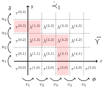
Figure 4. A random field of Young diagrams $\{\lambda^{(x,y)}\}$ with boundary conditions $\boldsymbol{\tau}$, and an example of a down-right path.

Definition 2.8.

A collection $\left\{(x_{i},y_{i})\right\}_{i=1}^{L}\subset\mathbb{Z}_{\geq 0}^{2}$, where $L\geq 1$, is called a down-right path if $x_{1}=0$, $y_{L}=0$, and the difference between consecutive vertices $(x_{i+1},y_{i+1})-(x_{i},y_{i})$ is either $(0,-1)$ or $(1,0)$ for all $i$.

Proposition 2.9.

Let $\boldsymbol{\lambda}$ be a field. Then the joint distribution of the Young diagrams along each down-right path $\left\{(x_{i},y_{i})\right\}_{i=1}^{L}$ conditioned on $\tau^{(0,y_{1})}$ and $\tau^{(x_{L},0)}$ has the form

$$\frac{1}{Z_{\mathrm{path}}}\,\prod_{i\colon y_{i+1}=y_{i}-1}\mathfrak{F}_{\lambda^{(x_{i},y_{i})}/\lambda^{(x_{i+1},y_{i+1})}}(u_{y_{i}})\prod_{i\colon x_{i+1}=x_{i}+1}\mathfrak{G}_{\lambda^{(x_{i+1},y_{i+1})}/\lambda^{(x_{i},y_{i})}}(v_{x_{i+1}}).$$ (2.10)

The normalizing constant has the form

$$Z_{\mathrm{path}}=Z^{(x_{L},y_{1})}_{\mathrm{boundary}}\prod_{\textnormal{$(x,y)$ below the path}}\Pi(u_{y};v_{x}).$$

Proof.

This follows by induction on flipping the down-right path using elementary steps $\llcorner\to\urcorner$ (i.e., by replacing the down-right corners by the right-down ones). The induction base is the path which first makes only down steps to $(0,0)$ and then only right steps. For this path the statement follows from the Gibbs property of the boundary condition (Definition 2.5).

The inductive step uses (2.9). Let us fix some $\llcorner$ corner $(x,y)$ in the path and use the notation of (2.9). Conditioned on $\lambda,\mu$, the Young diagram $\varkappa$ is independent of the diagram along the rest of the path. Using the induction assumption and (2.9) to replace the two factors corresponding to $(\lambda,\varkappa,\mu)$ in (2.10) by the ones corresponding to $(\lambda,\nu,\mu)$, we obtain the desired joint distribution along the modified down-right path. ∎

For the special choice of the path which first makes only right steps and then only down steps, we obtain with the help of the branching (2.2):

Corollary 2.10.

For any $x,y\geq 1$ we have

$$\mathop{\mathrm{Prob}}(\lambda^{(x,y)}\mid\tau^{(0,y)},\tau^{(x,0)})=\frac{\mathfrak{F}_{\lambda^{(x,y)}/\tau^{(x,0)}}(u_{1},\ldots,u_{y})\mathfrak{G}_{\lambda^{(x,y)}/\tau^{(0,y)}}(v_{1},\ldots,v_{x})}{Z^{(x,y)}}.$$ (2.11)

The normalizing constant has the form

$$Z^{(x,y)}=Z^{(x,y)}_{\mathrm{boundary}}\,\prod_{i=1}^{x}\prod_{j=1}^{y}\Pi(u_{y};v_{x}).$$

Note that for the step-type boundary conditions $\boldsymbol{\tau}$ there is no need to condition on the boundary values $\tau^{(0,y)}$ and $\tau^{(x,0)}$ in Proposition 2.9 and Corollary 2.10. For general Gibbs boundary conditions we have the following Gibbs preservation property:

Proposition 2.11.

For any $(x,y)\in\mathbb{Z}_{\geq 0}^{2}$, the two-sided sequence

$$\ldots\succ_{1}\lambda^{(x,y+2)}\succ_{1}\lambda^{(x,y+1)}\succ_{1}\lambda^{(x,y)}\mathop{\dot{\prec}_{1}}\lambda^{(x+1,y)}\mathop{\dot{\prec}_{1}}\lambda^{(x+2,y)}\mathop{\dot{\prec}_{1}}\ldots$$

is an $(\mathfrak{F},\mathfrak{G})$-Gibbs boundary condition in the sense of Definition 2.5.

Proof.

Immediately follows from Proposition 2.9. ∎

Example 2.12.

In the Schur case the distributions of Proposition 2.9 and Corollary 2.10 become the Schur processes and the Schur measures introduced in [OR03] and [Oko01], respectively (see also [BR05]). Early examples of random fields in this case were based on Robinson-Schensted-Knuth correspondences. Other approaches were suggested more recently in, e.g., [BF14], [WW09], [BP16a]. See Section 2.6 for more historical discussion.

2.4. Transition probabilities as bijectivizations of the skew Cauchy identity

Let us fix a skew Cauchy structure $(\mathfrak{F},\mathfrak{G})$, parameters (2.5), and a Gibbs boundary condition $\boldsymbol{\tau}$. Definition 2.5 does not characterize uniquely a random field $\boldsymbol{\lambda}$ corresponding to this data. Namely, consider any quadruple of neighboring Young diagrams (2.8) (related as in Figure 3) corresponding to $(x,y)\in\mathbb{Z}_{\geq 0}^{2}$. Given $\lambda,\mu$, condition (2.9) characterizes the marginal distributions of $\varkappa$ and $\nu$ separately. One readily sees that picking any joint distribution of $(\varkappa,\nu)$ given $\lambda,\mu$ with required marginals $\varkappa$ and $\nu$ produces a valid random field $\boldsymbol{\lambda}$ (and this choice can be made independently at every location $(x,y)$ in the quadrant). Therefore, one has to employ additional considerations to pick random fields with interesting properties, for example, possessing scalar Markovian marginals (see Section 2.5 below).

It is convenient to encode the choice of the joint distribution of $(\varkappa,\nu)$ given $\lambda$ and $\mu$ in an equivalent form of conditional probabilities. This leads to the following definition:

Definition 2.13.

Let $u,v\in\mathbb{C}$ be such that $(u,v)\in\mathsf{Adm}$, $u\in\mathsf{P}$, $v\in\dot{\mathsf{P}}$. The functions

$$\mathsf{U}^{\mathrm{fwd}}_{u,v}(\varkappa\to\nu\mid\lambda,\mu),\qquad\mathsf{U}^{\mathrm{bwd}}_{u,v}(\nu\to\varkappa\mid\lambda,\mu)$$

on quadruples of diagrams as in Figure 3 are called, respectively, the forward and the backward transition probabilities if:

1. The functions are nonnegative and sum to one over the second argument:

   $$\begin{split}\sum_{\nu}\mathsf{U}_{u,v}^{\mathrm{fwd}}(\varkappa\to\nu\mid\lambda,\mu)=1&\qquad\textnormal{for all triples $\lambda\succ_{1}\varkappa\mathop{\dot{\prec}_{1}}\mu$},\\ \sum_{\varkappa}\mathsf{U}_{u,v}^{\mathrm{bwd}}(\nu\to\varkappa\mid\lambda,\mu)=1&\qquad\textnormal{for all triples $\lambda\mathop{\dot{\prec}_{1}}\nu\succ_{1}\mu$.}\end{split}$$ (2.12)

   We will interpret $\mathsf{U}^{\mathrm{fwd}}(\varkappa\to\nu\mid\lambda,\mu)$ as a conditional distribution of $\nu$ given $\lambda\succ_{1}\varkappa\mathop{\dot{\prec}_{1}}\mu$, and $\mathsf{U}^{\mathrm{bwd}}$ as the opposite conditional distribution.

2. The functions satisfy the reversibility condition

   $$\mathsf{U}_{u,v}^{\mathrm{fwd}}(\varkappa\to\nu\mid\lambda,\mu)\cdot\Pi(u;v)\mathfrak{F}_{\lambda/\varkappa}(u)\mathfrak{G}_{\mu/\varkappa}(v)=\mathsf{U}_{u,v}^{\mathrm{bwd}}(\nu\to\varkappa\mid\lambda,\mu)\cdot\mathfrak{F}_{\nu/\mu}(u)\mathfrak{G}_{\nu/\lambda}(v).$$ (2.13)

Summing both sides of (2.13) over $\varkappa$ and $\nu$ produces the skew Cauchy identity (2.3). Therefore, choosing transition probabilities $\mathsf{U}^{\mathrm{fwd}}_{u,v}$ and $\mathsf{U}^{\mathrm{bwd}}_{u,v}$ corresponds to a refinement (“bijectivization”) of the skew Cauchy identity (for a general discussion of bijectivization, see Section 6.1 below). In the following sections we build bijectivizations of various concrete skew Cauchy identities out of bijectivizations of the Yang-Baxter equations.

Remark 2.14.

Summing (2.13) over $\varkappa$, we get

$$\Pi(u;v)\sum_{\varkappa}\mathsf{U}^{\mathrm{fwd}}_{u,v}(\varkappa\to\nu\mid\lambda,\mu)\cdot\mathfrak{F}_{\lambda/\varkappa}(u)\mathfrak{G}_{\mu/\varkappa}(v)=\mathfrak{F}_{\nu/\mu}(u)\mathfrak{G}_{\nu/\lambda}(v)$$ (2.14)

This identity was used in [BP16a] and [MP17] as a starting point to construct random fields associated with $q$-Whittaker functions. The advantage of (2.13) compared with (2.14) is that the former is more symmetric and does not involve summation.

Remark 2.15 (Borodin–Ferrari random fields).

The existence of at least one random field corresponding to a skew Cauchy structure $(\mathfrak{F},\mathfrak{G})$ is evident from the above discussion. An explicit basic construction of a field was suggested in [BF14] based on an idea of [DF90]. Namely, if $\mathsf{U}^{\mathrm{fwd}}(\varkappa\to\nu\mid\lambda,\mu)$ is independent of $\varkappa$, then by (2.14) it must have the form

$$\mathsf{U}_{u,v}^{\mathrm{fwd}}(\varkappa\to\nu\mid\lambda,\mu)=\frac{\mathfrak{F}_{\nu/\mu}(u)\mathfrak{G}_{\nu/\lambda}(v)}{\Pi(u;v)\sum_{\hat{\varkappa}}\mathfrak{F}_{\lambda/\hat{\varkappa}}(u)\mathfrak{G}_{\mu/\hat{\varkappa}}(v)}$$

if there exists $\hat{\varkappa}$ such that $\lambda\succ_{1}\hat{\varkappa}\mathop{\dot{\prec}_{1}}\mu$. Though this construction of a random field is rather simple and works in full generality for an arbitrary skew Cauchy structure, it does not produce all known examples of fields with scalar Markovian marginals. See Section 2.6 below for more discussion.

Using just the forward transition probabilities, start with arbitrary fixed (not necessarily Gibbs) boundary values $\lambda^{(x,0)}=\tau^{(x,0)}$ and $\lambda^{(0,y)}=\tau^{(0,y)}$, $x,y\geq 0$, and define a family of random Young diagrams $\{\lambda^{(x,y)}\}$ indexed by the quadrant as follows. By induction on $x+y=n$, assume that the Young diagrams with $x+y\leq n-1$ are determined. Then, independently for each $(x,y)$ with $x+y=n$ and $x,y\geq 1$ sample $\lambda^{(x,y)}$ having the distribution $\mathsf{U}^{\mathrm{fwd}}_{u_{y},v_{x}}(\lambda^{(x-1,y-1)}\to\lambda^{(x,y)}\mid\lambda^{(x,y+1)},\lambda^{(x+1,y)})$, where $\lambda^{(x-1,y-1)},\lambda^{(x,y+1)}$ and $\lambda^{(x+1,y)}$ are already determined. The next proposition immediately follows from the definitions:

Proposition 2.16.

If the boundary condition $\boldsymbol{\tau}$ in the above construction is Gibbs, then the resulting collection of random Young diagrams $\{\lambda^{(x,y)}\}$, $(x,y)\in\mathbb{Z}_{\geq 0}$ forms a random field in the sense of Definition 2.7.

Therefore, random fields associated with a skew Cauchy structure $(\mathfrak{F},\mathfrak{G})$ correspond to forward transition probabilities, and vice versa. Moreover, the probabilities $\mathsf{U}^{\mathrm{fwd}}_{u,v}$ allow to construct a joint distribution on Young diagrams $\{\lambda^{(x,y)}\}$ indexed by points of the quadrant $\mathbb{Z}_{\geq 0}^{2}$ starting from arbitrary boundary values. However, the Gibbs property on the boundary is needed for Proposition 2.9 describing joint distributions of the Young diagrams along down-right paths. We will not consider non-Gibbs boundary conditions in the present paper.

2.5. Scalar marginals

Let $\boldsymbol{\lambda}$ be a random field in the sense of Definition 2.7 and $\mathsf{h}\colon\mathbb{Y}\to\mathbb{Z}$ be a function. When the scalar random variables $\{\mathsf{h}(\lambda^{(x,y)})\}$ indexed by $(x,y)\in\mathbb{Z}_{\geq 0}^{2}$ evolve (in the sense of forward steps) independently of the rest of $\boldsymbol{\lambda}$, we call $\mathsf{h}(\boldsymbol{\lambda})$ a scalar (Markovian) marginal of a field $\boldsymbol{\lambda}$.

In detail, this independence means the following. For a finitely supported function $F$ on $\mathbb{Z}$ we can write for any field $\boldsymbol{\lambda}$:

$$\sum_{\nu\in\mathbb{Y}}F(\mathsf{h}(\nu))\,\mathsf{U}^{\mathrm{fwd}}_{u,v}(\varkappa\to\nu\mid\lambda,\mu)=\sum_{n\in\mathbb{Z}}F(n)\Bigg{(}\sum_{\nu\colon\mathsf{h}(\nu)=n}\mathsf{U}^{\mathrm{fwd}}_{u,v}(\varkappa\to\nu\mid\lambda,\mu)\Bigg{)}.$$ (2.15)

We say that the random field $\boldsymbol{\lambda}$ is $\mathsf{h}$-adapted if the quantity in the parentheses above

$$\mathsf{U}^{[\mathsf{h}]}_{u,v}(k\to n\mid\ell,m):=\sum_{\nu\colon\mathsf{h}(\nu)=n}\mathsf{U}^{\mathrm{fwd}}_{u,v}(\varkappa\to\nu\mid\lambda,\mu)$$ (2.16)

depends on $\lambda,\varkappa,\mu$ only through $\ell=\mathsf{h}(\lambda)$, $k=\mathsf{h}(\varkappa)$, and $m=\mathsf{h}(\mu)$. The function $\mathsf{U}^{[\mathsf{h}]}_{u,v}$ is nonnegative and $\sum_{n\in\mathbb{Z}}\mathsf{U}^{[\mathsf{h}]}_{u,v}(k\to n\mid\ell,m)=1$ for all $\ell,k,m$ such that there exists at least one triple $\lambda\succ_{1}\varkappa\mathop{\dot{\prec}_{1}}\mu$. In words, to sample $\nu$ knowing $\lambda,\varkappa,\mu$ we first look at $\ell,k,m$ and sample $n=\mathsf{h}(\nu)$ independently of any other information about the diagrams $\lambda,\varkappa,\mu$, and then sample the rest of the diagram $\nu$.

For a $\mathsf{h}$-adapted field $\boldsymbol{\lambda}$, the joint distribution of the scalar quantities $\mathsf{h}(\lambda^{(x,y)})$, $(x,y)\in\mathbb{Z}_{\geq 0}^{2}$ (forming the scalar marginal of $\boldsymbol{\lambda}$ corresponding to $\mathsf{h}$), can be described using (2.16) as forward transition probabilities:

$$\mathop{\mathrm{Prob}}\left(\mathsf{h}(\lambda^{(x+1,y+1)})=n\,\Big{|}\,\mathsf{h}(\lambda^{(x,y+1)})=\ell,\mathsf{h}(\lambda^{(x,y)})=k,\mathsf{h}(\lambda^{(x+1,y)})=m,\right)\\ =\mathsf{U}^{[\mathsf{h}]}_{u_{y+1},v_{x+1}}(k\to n\mid\ell,m).$$

Note that while for a scalar marginal $\mathsf{h}$ the forward transition probabilities factorize as in (2.15)–(2.16), the backward ones do not have to factorize in the same way.

Remark 2.17.

One can take an arbitrary set instead of $\mathbb{Z}$ as the target of $\mathsf{h}$ as this is essentially the index set of equivalence classes of Young diagrams. In the rest of the paper we mostly focus on integer-valued scalar Markovian marginals, but also mention their higher-dimensional (multilayer) extensions obtained by refining these equivalence classes.

Scalar marginals in the Schur case (our running example) are discussed in the next Section 2.6.

2.6. Existing constructions of random fields

This subsection is a brief review of known random fields associated with skew Cauchy structures corresponding to various families of symmetric functions (see Figure 1 for the hierarchy of symmetric functions we mention below).

Constructing probability measures on Young diagrams related to the Schur symmetric functions by means of Markov dynamics on Young tableaux goes back at least to [VK86]. The first such mechanism employed in many well-known developments in Integrable Probability starting from [BDJ99] and [Joh00] is the Robinson-Schensted-Knuth (RSK) correspondence. In particular, the RSK gives rise to a random field of Young diagrams associated with Schur functions whose scalar marginal field is identified with the Totally Asymmetric Simple Exclusion Process (TASEP). The distributions in TASEP started from a special initial configuration called “step” (when the particles occupy the negative half-line while the positive half-line is empty) are then related to the Schur measures and processes introduced in [Oko01], [OR03]. The corresponding field of random Young diagrams in this case has step-type Gibbs boundary condition in the sense of our Definition 2.6. Further applications of RSK and its tropical version to particle systems, last passage percolation models, and random polymers were developed in [O’C03a], [O’C03], [BBO05], [Chh13], [O’C12], [COSZ14], [OSZ14], and related works.

Another mechanism of constructing random fields associated with Schur polynomials was suggested in [BF14], see also [Bor11]. (We outlined this construction in Remark 2.15.) This mechanism was later employed in [BC14] to discover the (continuous-time) $q$-deformation of the TASEP as a scalar marginal in a field associated with the $q$-Whittaker functions. The integrable structure of the $q$-TASEP is based on the $q$-difference operators diagonal in the $q$-Whittaker polynomials (these are the $t=0$ Macdonald difference operators [Mac95, Chapter VI.3]). It soon became apparent, however, that Borodin–Ferrari random fields cannot produce all known integrable stochastic particle systems on the line as their Markovian marginals. Early examples of stochastic particle systems not coming out of Borodin–Ferrari fields include the discrete-time $q$-TASEPs suggested in [BC15].

This issue motivated the search for other constructions of random fields, and resulted in discovery of $q$-Whittaker and Hall-Littlewood randomizations of the RSK correspondence [OP13], [BP16a], [BP15], [MP17], [BM18]. On the $q$-Whittaker side, this brought new $q$-TASEPs and $q$-PushTASEPs whose distributions are expressed through the $q$-Whittaker measures and processes. The Hall-Littlewood side brought the integrable structure of Hall-Littlewood measures and processes to the stochastic six vertex model and the ASEP (i.e, TASEP with left and right jumps allowed).

In parallel to these developments a new extension of the $q$-TASEP called the $q$-Hahn TASEP was invented [Pov13], [Cor14]. Further investigation of this process has led to the systematic development of the spin Hall-Littlewood (sHL) symmetric rational functions and the associated stochastic vertex models [BCPS15], [Bor17], [CP16], [BP16], [BP18]. In particular, the Yang-Baxter equation for the higher spin six vertex model implies the skew Cauchy identity for the sHL functions. Recently, the spin $q$-Whittaker (sqW) symmetric polynomials were introduced in [BW17] as the dual complement (which for $s=0$ reduces to the $q\leftrightarrow t$ Macdonald involution) of the sHL ones.

These new skew Cauchy structures called for extending the random field constructions which would bring interesting scalar marginals. In [BP17] this was performed in the sHL setting based on a new idea of bijectivization of the Yang-Baxter equation (we recall it in Section 6 below). This idea allowed to bypass technical difficulties associated with randomizing the RSKs and, on the other hand, by design has produced a scalar marginal of the sHL Yang-Baxter field which is a new dynamical extension of the stochastic six vertex model. In this paper we complete the picture by constructing Yang-Baxter fields associated with two other skew Cauchy structures corresponding to the sqW/sHL and the sqW/sqW skew Cauchy identities (see Section 7), and find that their scalar marginals are related to the stochastic higher spin six vertex model of [CP16], [BP18] and to the $q$-Hahn PushTASEP recently introduced in [CMP18]. In Section 8 we employ the former connection to discover new difference operators acting diagonally on sqW or stable sHL functions.

Remark 2.18.

One can also define the notion of a random field of Young diagrams associated with Macdonald or Jack symmetric functions since they, too, satisfy skew Cauchy identities. However, due to the more complicated “nonlocal” structure of the Jack and Macdonald Pieri rules compared to the $q$-Whittaker or Hall-Littlewood ones, it seems unlikely that there exist Jack or Macdonald random fields with scalar Markovian marginals. In this paper we do not focus on this question.

3. Spin Hall-Littlewood and spin $q$-Whittaker functions

In this section we review the main properties of the stable spin Hall-Littlewood and spin $q$-Whittaker symmetric functions [Bor17], [BW17] which lead to skew Cauchy structures. These functions are defined as partition functions of certain ensembles of lattice paths realized through a vertex model formalism. We fix the main “quantization” parameter $q\in(0,1)$. In contrast with Figure 1, throughout the text we use $q$ to denote the quantization parameter in both spin Hall-Littlewood and spin $q$-Whittaker functions, which is convenient when considering Yang-Baxter fields based on both families.

3.1. Young diagrams as arrow configurations

We represent Young diagrams $\lambda=(\lambda_{1}\geq\ldots\geq\lambda_{\ell(\lambda)}>0)$ as configurations of vertical arrows on $\mathbb{Z}_{\geq 0}$. Let $\lambda$ be written in the multiplicative notation as $\lambda=1^{l_{1}}2^{l_{2}}\ldots$, where $l_{i}$ is the number of parts of $\lambda$ which are equal to $i$. By definition, the arrow configuration corresponding to $\lambda$, denoted by $|\lambda\rangle$, contains $l_{i}$ vertical arrows at location $i$. The number of vertical arrows at $0$ is assumed infinite which reflects the fact that one can append Young diagrams by zeros without changing them. See Figure 5, left, for an illustration.

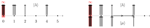
Figure 5. Left: Configuration $|\lambda\rangle$ of vertical arrows corresponding to the Young diagram $\lambda=(4,4,2,1,1,1)$. Right: Interlacing of $\lambda$ with $\mu=(4,2,2,1,1,1)$.

3.2. Stable spin Hall-Littlewood functions

The first collection of vertex weights we work with is given in Figure 6. Along with $q$, these weights depend on two quantities $u,s\in\mathbb{C}$, which are called the spectral and the spin parameters, respectively. The weights $w_{u,s}$ satisfy the Yang-Baxter equation, see Appendix A.

$w_{u,s}(i_{1},j_{1};i_{2},j_{2})$	$\frac{1-suq^{g}}{1-su}$	$\frac{u(1-s^{2}q^{g})}{1-su}$	$\frac{u-sq^{g}}{1-su}$	$\frac{1-q^{g+1}}{1-su}$

Figure 6. In the top row we see all acceptable configurations of arrows entering and exiting a vertex; below we reported the corresponding vertex weights $w_{u,s}(i_{1},j_{1};i_{2},j_{2})$.

For vertices at the left boundary we set

$$w_{u,s}\biggl{(}\leavevmode\hbox to28.45pt{\vbox to33.73pt{\text{[drawing]}}}\biggr{)}=w_{u,s}(\infty,\varnothing;\infty,1)=u,\qquad w_{u,s}\biggl{(}\leavevmode\hbox to28.45pt{\vbox to33.73pt{\text{[drawing]}}}\biggr{)}=w_{u,s}(\infty,\varnothing;\infty,0)=1, \infty \infty \infty \infty \infty \infty \infty \infty$$ (3.1)

Both in Figure 6 and in (3.1), we attribute weight zero to all configurations which are not listed. In particular, the following arrow conservation property holds:

$$w_{u,s}(i_{1},j_{1};i_{2},j_{2})=0\qquad\textnormal{unless $i_{1}+j_{1}=i_{2}+j_{2}$}.$$ (3.2)

Definition 3.1 (Interlacing).

Fix $\mu,\lambda\in\mathbb{Y}$. We say that $\mu$ and $\lambda$ interlace (notation $\mu\prec\lambda$) if there exists a configuration of finitely many horizontal arrows between $|\mu\rangle$ and $|\lambda\rangle$ as in Figure 5, right, such that the arrow conservation property holds at each vertex. In detail, $\mu\prec\lambda$ if either of the two hold:

$$\begin{split}&\ell(\lambda)=\ell(\mu)\text{ and }\mu_{\ell(\mu)}\leq\lambda_{\ell(\lambda)}\leq\ldots\leq\lambda_{2}\leq\mu_{1}\leq\lambda_{1},\\ &\ell(\lambda)=\ell(\mu)+1\text{ and }\lambda_{\ell(\lambda)}\leq\mu_{\ell(\mu)}\leq\lambda_{\ell(\lambda)-1}\leq\ldots\leq\lambda_{2}\leq\mu_{1}\leq\lambda_{1}.\end{split}$$ (3.3)

Note that for each $\lambda\in\mathbb{Y}$, the number of $\mu$ such that $\mu\prec\lambda$ is finite.

Definition 3.2.

For $\mu,\lambda\in\mathbb{Y}$ with $\mu\prec\lambda$, a stable spin Hall-Littlewood function in one variable, denoted by $\mathsf{F}_{\lambda/\mu}(u)$, is defined as the total weight (= product of individual vertex weights) of the unique configuration of arrows between $|\mu\rangle$ and $|\lambda\rangle$ as in Figure 5, right. Here the individual vertex weights are the $w_{u,s}$’s from Figure 6, and the left boundary weights are (3.1). If $\mu\not\prec\lambda$, we set $\mathsf{F}_{\lambda/\mu}(u)=0$.

In the sequel we will mostly omit the word “stable” (cf. Section 3.3 on connections to the non-stable functions which were originally defined in [Bor17]), and will also abbreviate the name to simply the sHL functions.

Define the functions with multiple variables inductively via the branching rule (cf. (2.2)):

$$\mathsf{F}_{\lambda/\mu}(u_{1},\dots,u_{k})=\sum_{\nu}\mathsf{F}_{\lambda/\nu}(u_{k})\,\mathsf{F}_{\nu/\mu}(u_{1},\dots,u_{k-1}).$$ (3.4)

That is, $\mathsf{F}_{\lambda/\mu}(u_{1},\ldots,u_{k})$ is a partition function of ensembles of up-right paths as in Figure 7, left, with height $k$, spectral parameters $u_{1},\ldots,u_{k}$ corresponding to horizontal slices, and boundary conditions $|\mu\rangle$, $0^{\infty}$, $|\lambda\rangle$ and empty at the bottom, left, up, and right, respectively. The fact that the paths are directed up-right corresponds to the arrow conservation property (3.2). Note that $\mathsf{F}_{\lambda/\mu}(u_{1},\ldots,u_{k})$ vanishes unless $0\leq\ell(\lambda)-\ell(\mu)\leq k$, but this condition is not sufficient.

The Yang-Baxter equation implies that $\mathsf{F}_{\lambda/\mu}(u_{1},\ldots,u_{k})$ is symmetric with respect to permutations of the $u_{i}$’s, see, e.g., [Bor17, Theorem 3.6]. These functions also satisfy the stability property

$$\mathsf{F}_{\lambda/\mu}(u_{1},\ldots,u_{k},0)=\mathsf{F}_{\lambda/\mu}(u_{1},\ldots,u_{k}).$$ (3.5)

For $\mu=\varnothing$, the stable spin Hall-Littlewood functions admit an explicit symmetrization formula [BW17, (45)] which we recall and use in Section 8. When $s=0$, the stable spin Hall-Littlewood functions become the usual Hall-Littlewood symmetric polynomials [Mac95, Chapter III].

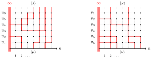
Figure 7. Examples of configurations of up-right and down-right paths used in the definitions of $\mathsf{F}_{\lambda/\mu}$ and $\mathsf{F}^{*}_{\nu/\varkappa}$, respectively.

3.3. Remark. Relations to non-stable sHL functions

The spin Hall-Littlewood functions were originally introduced in [Bor17] in their non-stable version which we denote by $\mathsf{F}^{\textnormal{non-st}}_{\lambda/\mu}$. The stable modification appeared in [GGW17] and [BW17]. The non-stable sHL functions differ by the boundary condition on the left: a new horizontal arrow enters at each horizontal slice and each vertical edge on the leftmost column hosts only finitely many arrows.

In detail, the definition of $\mathsf{F}^{\textnormal{non-st}}_{\lambda/\mu}$ depends on the number of zero parts in $\lambda=0^{l_{0}}1^{l_{1}}2^{l_{2}}\ldots$ and $\mu=0^{m_{0}}1^{m_{1}}2^{m_{2}}\ldots$, and $\mathsf{F}^{\textnormal{non-st}}_{\lambda/\mu}(u)$ vanishes unless $l_{0}+l_{1}+\ldots=1+m_{0}+m_{1}+\ldots$. When the latter condition holds, we define the single-variable function $\mathsf{F}^{\textnormal{non-st}}_{\lambda/\mu}(u)$ as the weight of the unique configuration as in Definition 3.2, but now the horizontal arrow must enter at the leftmost boundary, and the vertex weight at the zeroth column is $w_{u,s}(m_{0},1;l_{0},m_{0}+1-l_{0})$. The multivariable version is defined using the branching rule exactly as in (3.4).

There are two possible ways one could specialize the non-stable sHL functions to obtain our $\mathsf{F}_{\lambda/\mu}$. The first is to send both $l_{0}$ and $m_{0}$, the numbers of zeros in $\lambda$ and $\mu$, to infinity. By looking at the weight of the leftmost vertices we see that

$$w_{u,s}(m_{0},1;l_{0},j)\xrightarrow[m_{0},l_{0}\to\infty]{}\frac{u^{j}}{1-su},\qquad j\in\{0,1\},$$

and therefore we obtain

$$\mathsf{F}_{\lambda/\mu}(u_{1},\ldots,u_{k})=\prod_{i=1}^{k}(1-su_{i})\times\lim_{m_{0},l_{0}\to\infty}\mathsf{F}_{\lambda\cup 0^{l_{0}}/\mu\cup 0^{m_{0}}}^{\textnormal{non-st}}(u_{1},\ldots,u_{k}).$$ (3.6)

Here $\lambda\cup 0^{l_{0}}$ means adding $l_{0}$ zeros to the Young diagram $\lambda$ (which had no zeros originally), and similarly for $\mu\cup 0^{m_{0}}$.

Another way is to consider the inhomogeneous vertex model as in [BP18] with the spin parameter $s_{n}$, $n\in\mathbb{Z}_{\geq 0}$, depending on the horizontal coordinate $n$ in Figure 7. Taking $\mathsf{F}_{\lambda/\mu}^{\textnormal{non-st}}$ and setting $s_{0}=0$ and $s_{n}=s$, $n>0$, from Figure 6 we see that

$$w_{u,0}(i_{1},1;i_{2},0)=1-q^{i_{2}}\qquad\text{and}\qquad w_{u,0}(i_{1},1;i_{2},1)=u.$$

Therefore, we obtain

$$\mathsf{F}_{\lambda/\mu}(u_{1},\dots,u_{k})=\frac{1}{(q;q)_{k-\ell(\lambda)+\ell(\mu)}}\,\mathsf{F}^{\textnormal{non-st}}_{\lambda\cup 0^{k-\ell(\lambda)+\ell(\mu)}/\mu}(u_{1},\dots,u_{k})\Big{|}_{s_{0}=0},$$ (3.7)

where we assume that $\mu,\lambda$ had no zeros originally. Equality (3.7) is particularly useful when adapting the results about the non-stable sHL functions (like symmetrization formulas or integral representations [Bor17], [BP18]) to the stable case.

3.4. Dual stable spin Hall-Littlewood functions

Let us introduce the dual weights to $w_{u,s}$ from Figure 6 as follows:

$$w^{*}_{v,s}(i_{1},j_{1};i_{2},j_{2})=\frac{(s^{2};q)_{i_{1}}(q;q)_{i_{2}}}{(q;q)_{i_{1}}(s^{2};q)_{i_{2}}}\,w_{v,s}(i_{2},j_{1};i_{1},j_{2}).$$ (3.8)

The arrow conservation law (3.2) implies that $w_{v,s}^{*}(i_{1},j_{1};i_{2},j_{2})$ vanishes unless $i_{2}+j_{1}=i_{1}+j_{2}$, and as a result the corresponding vertex model produces configurations of directed down-right paths (see Figure 7, right). The explicit form of the weights $w_{v,s}^{*}$ is given in Figure 8.

$w^{*}_{v,s}(i_{1},j_{1};i_{2},j_{2})$	$\frac{1-svq^{g}}{1-sv}$	$\frac{1-s^{2}q^{g}}{1-sv}$	$\frac{v-sq^{g}}{1-sv}$	$\frac{(1-q^{g+1})v}{1-sv}$

Figure 8. In the top row we see all acceptable configurations of paths entering and exiting a vertex; below we reported the corresponding vertex weights $w^{*}_{v,s}(i_{1},j_{1};i_{2},j_{2})$.

The weights $w^{*}_{v,s}$ at the left boundary are given by the same formulas as in (3.1).

The weights $w^{*}_{v,s}$ can be obtained from $w_{u,s}$ by substituting $u$ with $1/v$, swapping the values of both horizontal edge indices $j_{1}$ and $j_{2}$ (that is if $j_{1}=0$, then we change its value 1 and vice versa, and the same for $j_{2}$), and multiplying the result by $(v-s)/(1-vs)$. This swapping construction of the dual weights was instrumental in deriving Cauchy identities for the sHL functions from the Yang-Baxter equation [Bor17] (a bijectivization of this argument appeared in [BP17]). In the present paper we employ a more direct approach with down-right paths which is better suited for the generalization to spin $q$-Whittaker functions. The Yang-Baxter equation connecting $w_{u,s}$ and $w^{*}_{v,s}$ is recorded in Appendix A.

Definition 3.3.

Fix $\varkappa,\nu\in\mathbb{Y}$ with $\varkappa\prec\nu$ and place the arrow configuration $|\nu\rangle$ under $|\varkappa\rangle$. Then there exists a unique configuration of horizontal arrows between $|\varkappa\rangle$ and $|\nu\rangle$. By definition, a dual stable sHL function in one variable, denoted by $\mathsf{F}_{\nu/\varkappa}^{*}(v)$, is the total weight of this horizontal arrow configuration, where the individual vertex weights are the $w^{*}_{v,s}$’s from Figure 8, and the left boundary weights are the same as in (3.1). If $\varkappa\not\prec\nu$, we set $\mathsf{F}^{*}_{\nu/\varkappa}(v)=0$.

The multivariable generalization $\mathsf{F}^{*}_{\nu/\varkappa}(v_{1},\ldots,v_{k})$ is defined via the branching rule exactly as in (3.4). It is the partition function of ensembles of down-right paths as in Figure 7, right, of height $k$, spectral parameters $v_{1},\ldots,v_{k}$ corresponding to horizontal slices, and boundary conditions $|\varkappa\rangle$, $0^{\infty}$, $|\nu\rangle$, and empty at the bottom, left, top, and right, respectively.

The relation (3.8) between $w^{*}_{v,s}$ and $w_{u,s}$ implies that

$$\frac{\mathsf{c}(\lambda)}{\mathsf{c}(\mu)}\,\mathsf{F}_{\lambda/\mu}(u_{1},\dots,u_{k})=\mathsf{F}^{*}_{\lambda/\mu}(u_{1},\dots,u_{k}),$$ (3.9)

where the factor $\mathsf{c}$ is

$$\mathsf{c}(\mu)=\prod_{i\geq 1}\frac{(s^{2};q)_{m_{i}}}{(q;q)_{m_{i}}},\qquad\text{for }\mu=1^{m_{1}}2^{m_{2}}\ldots.$$

The symmetry of $\mathsf{F}^{*}_{\lambda/\mu}(v_{1},\ldots,v_{k})$ in the $v_{i}^{\prime}s$ follows from the symmetry of $\mathsf{F}_{\lambda/\mu}$. The dual sHL function also satisfies the same stability property (3.5) as the non-dual one.

3.5. The sHL/sHL skew Cauchy structure

One of the main consequences of the Yang-Baxter equation (either Proposition A.1 or Proposition A.2) is the skew Cauchy identity for the sHL functions:

Theorem 3.4 ([Bor17], [BP18], [BW17, Section 7.4]).

For any two Young diagrams $\lambda,\mu$ and generic parameters $u,v\in\mathbb{C}$ (cf. Remark 2.1) such that $\bigl{|}(u-s)(v-s)\bigr{|}<\bigl{|}(1-su)(1-sv)\bigr{|}$, we have

$$\sum_{\nu}\mathsf{F}^{*}_{\nu/\lambda}(v)\,\mathsf{F}_{\nu/\mu}(u)=\frac{1-quv}{1-uv}\sum_{\varkappa}\mathsf{F}_{\lambda/\varkappa}(u)\,\mathsf{F}^{*}_{\mu/\varkappa}(v).$$ (3.10)

We recall a “bijective” proof of Theorem 3.4 in Section 7.2 below which follows the approach of [BP17]. This identity together with the branching rules for the sHL functions lead to the first of the skew Cauchy structures we consider in the paper:

Definition 3.5.

The families of functions

$$\mathfrak{F}_{\lambda/\mu}(u_{1},\ldots,u_{k})=\mathsf{F}_{\lambda/\mu}(u_{1},\ldots,u_{k}),\qquad\mathfrak{G}_{\lambda/\mu}(v_{1},\ldots,v_{k})=\mathsf{F}^{*}_{\lambda/\mu}(v_{1},\ldots,v_{k})$$

form a skew Cauchy structure in the sense of Section 2.1 with the following identifications:

1. The relations $\mu\prec_{k}\lambda$ and $\mu\mathop{\dot{\prec}_{k}}\lambda$ are the same and mean the existence of a sequence of Young diagrams $\mu\prec\varkappa^{(1)}\prec\ldots\prec\varkappa^{(k-1)}\prec\lambda$, where $\prec$ is the interlacing relation (3.3).

2. The skew Cauchy identity holds with

   $$\mathsf{Adm}=\left\{(u,v)\colon\bigl{|}(u-s)(v-s)\bigr{|}<\bigl{|}(1-su)(1-sv)\bigr{|}\right\},\qquad\Pi(u;v)=\dfrac{1-quv}{1-uv}.$$ (3.11)

3. Let us choose the external parameters $q\in(0,1)$, $s\in(-1,0)$, and take $\mathsf{P}=\dot{\mathsf{P}}=[0,1]$. Then the probability weights based on $\mathsf{F}_{\lambda/\mu}(u_{1},\ldots,u_{k})$ and $\mathsf{F}^{*}_{\lambda/\mu}(v_{1},\ldots,v_{k})$ with $u_{i},v_{j}\in[0,1]$ are nonnegative due to the nonnegativity of all the vertex weights in Figures 6 and 8.

We call this the sHL/sHL skew Cauchy structure.

Remark 3.6.

When $u,v\in[0,1)$ and $s\in(-1,0)$, one can check that $(u,v)\in\mathsf{Adm}$.

3.6. Spin $q$-Whittaker polynomials

Along with the sHL functions we will work with the spin $q$-Whittaker (sqW) polynomials introduced in [BW17] which we recall here. We start by defining the vertex weights $W_{\xi,s}$ as

$$W_{\xi,s}(i_{1},j_{1};i_{2},j_{2})=\mathbf{1}_{i_{1}+j_{1}=i_{2}+j_{2}}\,\mathbf{1}_{i_{1}\geq j_{2}}\,\xi^{j_{2}}\,\frac{(-s/\xi;q)_{j_{2}}(-s\xi;q)_{i_{1}-j_{2}}(q;q)_{i_{2}}}{(q;q)_{j_{2}}(q;q)_{i_{1}-j_{2}}(s^{2};q)_{i_{2}}},$$ (3.12)

where $i_{1},j_{1},i_{2},j_{2}\in\mathbb{Z}_{\geq 0}$. Note that in contrast with $w_{u,s}$ and $w^{*}_{v,s}$ used in the definition of the sHL functions, here the number of horizontal arrows $j_{1},j_{2}$ can be arbitrary and not just zero or one.

The dual version of the weight $W_{\xi,s}$ is given by

$$W^{*}_{\theta,s}(i_{1},j_{1};i_{2},j_{2})=\frac{(s^{2};q)_{i_{1}}(q;q)_{i_{2}}}{(q;q)_{i_{1}}(s^{2};q)_{i_{2}}}\,W_{\theta,s}(i_{2},j_{1};i_{1},j_{2}),$$ (3.13)

which is the same relation as between $w$ and $w^{*}$ (3.8). The weights $W^{*}_{\theta,s}$ vanish unless $i_{2}+j_{1}=i_{1}+j_{2}$, therefore the dual vertex model will have down-right paths. The dependence of both $W_{\xi,s}$ and $W^{*}_{\theta,s}$ on their respective spectral parameters $\xi,\theta$ is polynomial.

As explained in Appendix A, there exists a close relation between the weights $W$ and the weights $w$: the former can be obtained from the latter through a procedure called fusion. The fusion consists in collapsing multiple $w$-weighted rows of vertices with spectral parameters forming a geometric progression with ratio $q$ Fusion originated in [KRS81] and was employed in [Bor17], [CP16], [BP18], [BW17] in connection with stochastic vertex models. In particular, the weights $W_{\xi,s}$ and $W^{*}_{\theta,s}$ satisfy the Yang-Baxter equation listed in Appendix A.

Define the left boundary weights for $j\in\mathbb{Z}_{\geq 0}$ by

$$W_{\xi,s}\biggl{(}\leavevmode\hbox to39.81pt{\vbox to33.73pt{\text{[drawing]}}}\biggr{)}=W_{\xi,s}^{*}\biggl{(}\leavevmode\hbox to39.81pt{\vbox to33.73pt{\text{[drawing]}}}\biggr{)}=\xi^{j}\,\frac{(-s/\xi;q)_{j}}{(q;q)_{j}}.\qquad \infty \infty j \infty \infty j \infty \infty j \infty \infty j$$ (3.14)

Definition 3.7 (Column interlacing).

Fix $\mu,\lambda\in\mathbb{Y}$. We write $\mu\mathop{\prec^{\prime}}\lambda$ and say that $\mu$ and $\lambda$ column-interlace if there exists a configuration of finitely many horizontal arrows between $|\mu\rangle$ and $|\lambda\rangle$ (located one under another as in Figure 5) such that at each vertex $(i_{1},j_{1};i_{2},j_{2})$ the arrow conservation property $i_{1}+j_{1}=i_{2}+j_{2}$ holds, and, moreover, $j_{2}\leq i_{1}$. Note that now we allow arbitrarily many horizontal arrows per edge. (If such a horizontal arrow configuration exists, then it is unique.) One can check that $\mu\mathop{\prec^{\prime}}\lambda$ if and only if $\mu^{\prime}\prec\lambda^{\prime}$, where $\mu^{\prime}$ and $\lambda^{\prime}$ stand for transposed Young diagrams:

$$\lambda^{\prime}_{j}:=\#\left\{i\colon\lambda_{i}\geq j\right\}.$$

Definition 3.8.

For $\mu,\lambda\in\mathbb{Y}$ with $\mu\prec^{\prime}\lambda$, a spin $q$-Whittaker polynomial in one variable, denoted by $\mathbb{F}_{\lambda^{\prime}/\mu^{\prime}}(\xi)$, is defined as the total weight of the unique configuration of arrows between $|\mu\rangle$ and $|\lambda\rangle$. Here the individual vertex weights are $W_{\xi,s}$ (3.12), (3.14). If $\mu\not\prec^{\prime}\lambda$, we set $\mathbb{F}_{\lambda^{\prime}/\mu^{\prime}}(\xi)=0$.

We will abbreviate the name and call $\mathbb{F}_{\lambda^{\prime}/\mu^{\prime}}$ simply the (skew) sqW polynomial. Note that it is indexed by the transposed Young diagrams for consistency with the $s=0$ situation when $\mathbb{F}_{\lambda^{\prime}/\mu^{\prime}}$ turns into the more common skew $q$-Whittaker polynomial which is a $t=0$ degeneration of the corresponding Macdonald polynomial [Mac95], [BC14].

The dual sqW polynomials $\mathbb{F}_{\nu/\varkappa}^{*}(\theta)$ are defined in a similar manner, up to placing $|\nu\rangle$ under $|\varkappa\rangle$, and using the dual vertex weights $W^{*}_{\theta,s}$ (3.13), (3.14). We have (cf. (3.9))

$$\frac{\mathsf{c}(\nu)}{\mathsf{c}(\varkappa)}\,\mathbb{F}_{\nu^{\prime}/\varkappa^{\prime}}(\xi_{1},\ldots,\xi_{k})=\mathbb{F}_{\nu^{\prime}/\varkappa^{\prime}}^{*}(\xi_{1},\ldots,\xi_{k}).$$ (3.15)

The multivariable polynomials $\mathbb{F}_{\lambda/\mu}(\xi_{1},\ldots,\xi_{k})$ and $\mathbb{F}^{*}_{\nu/\varkappa}(\theta_{1},\ldots,\theta_{k})$ are defined via the branching rules exactly as in (3.4). One can view them as partition functions of path ensembles similarly to the ones in Figure 7, but with multiple horizontal arrows allowed per edge. The Yang-Baxter equation implies that $\mathbb{F}_{\lambda/\mu}(\xi_{1},\ldots,\xi_{k})$ and $\mathbb{F}^{*}_{\nu/\varkappa}(\theta_{1},\ldots,\theta_{k})$ are symmetric in their respective variables. They also satisfy the following stability property:

$$\mathbb{F}_{\lambda/\mu}(\xi_{1},\ldots,\xi_{k-1},-s)=\mathbb{F}_{\lambda/\mu}(\xi_{1},\ldots,\xi_{k-1})$$

(and similarly for $\mathbb{F}_{\nu/\varkappa}^{*}$), which follows from the vanishing of the vertex weight $W_{-s,s}$. Note that here we are substituting $(-s)$ for one of the variables in contrast with the sHL functions where we substituted $0$ (3.5).

3.7. The sHL/sqW skew Cauchy structure

The Yang-Baxter equation for the weights $(w^{*}_{v,s},W_{\xi,s})$, see Proposition A.6, implies the following “dual” skew Cauchy identity for the sHL and sqW functions:

Theorem 3.9 ([BW17, Section 7.3]).

For any two Young diagrams $\lambda,\mu$, and generic $\xi,u\in\mathbb{C}$ (cf. Remark 2.1; in particular, $u\neq s^{-1}$) we have

$$\begin{split}\sum_{\nu}\mathbb{F}_{\nu^{\prime}/\lambda^{\prime}}(\xi)\,\mathsf{F}^{*}_{\nu/\mu}(u)&=\frac{1+u\xi}{1-us}\sum_{\varkappa}\mathbb{F}_{\mu^{\prime}/\varkappa^{\prime}}(\xi)\,\mathsf{F}^{*}_{\lambda/\varkappa}(u);\\ \sum_{\nu}\mathbb{F}^{*}_{\nu^{\prime}/\lambda^{\prime}}(\xi)\,\mathsf{F}_{\nu/\mu}(u)&=\frac{1+u\xi}{1-us}\sum_{\varkappa}\mathbb{F}^{*}_{\mu^{\prime}/\varkappa^{\prime}}(\xi)\,\mathsf{F}_{\lambda/\varkappa}(u).\end{split}$$ (3.16)

Note that the sums over $\nu$ and $\varkappa$ in both sides are actually finite, so there are no convergence issues. The above two identities are equivalent: One can multiply the first one by $\mathsf{c}(\mu)/\mathsf{c}(\lambda)$ and redistribute the factors to get the second one.

We give a “bijective” proof of Theorem 3.9 in Section 7.3 below. This leads to the following definition:

Definition 3.10.

The families of functions $\mathfrak{F}_{\lambda/\mu}(u_{1},\ldots u_{k})=\mathsf{F}^{*}_{\lambda/\mu}(u_{1},\ldots,u_{k})$ and $\mathfrak{G}_{\lambda/\mu}(\xi_{1},\ldots,\xi_{k})=\mathbb{F}_{\lambda^{\prime}/\mu^{\prime}}(\xi_{1},\ldots,\xi_{k})$ form a skew Cauchy structure in the sense of Section 2.1 with the following identifications:

1. The relations $\prec_{k}$, $\mathop{\dot{\prec_{k}}}$ on $\mathbb{Y}\times\mathbb{Y}$ are

   $$\begin{split}\mu\prec_{k}\lambda\qquad\Leftrightarrow\qquad&\exists\,\varkappa^{(i)}\in\mathbb{Y}\colon\mu\prec\varkappa^{(1)}\prec\ldots\prec\varkappa^{(k-1)}\prec\lambda;\\ \mu\mathop{\dot{\prec}_{k}}\lambda\qquad\Leftrightarrow\qquad&\exists\,\rho^{(j)}\in\mathbb{Y}\colon\mu\prec^{\prime}\rho^{(1)}\prec^{\prime}\ldots\prec^{\prime}\rho^{(k-1)}\prec^{\prime}\lambda,\end{split}$$

   where $\prec$ and $\prec^{\prime}$ are the usual and the column interlacing relations (Definitions 3.1 and 3.7).

2. The skew Cauchy identity holds with $\mathsf{Adm}=\left\{(u,\xi)\in\mathbb{C}^{2}\colon u\neq s^{-1}\right\}$ and

   $$\Pi(u;\xi)=\dfrac{1+u\xi}{1-su}.$$ (3.17)

3. The external parameters of the functions are $q\in(0,1)$ and $s\in(-1,0)$, and the nonnegativity sets for the spectral parameters are $\mathsf{P}=[0,1]$, $\dot{\mathsf{P}}=[-s,-s^{-1}]$. Then the probability weights based on $\mathsf{F}^{*}_{\lambda/\mu}(u_{1},\ldots,u_{k})$ and $\mathbb{F}_{\lambda^{\prime}/\mu^{\prime}}(\xi_{1},\ldots,\xi_{k})$ are nonnegative for $u_{i}\in\mathsf{P}$, $\xi_{j}\in\dot{\mathsf{P}}$ due to the nonnegativity of the vertex weights in Figure 8 and (3.12).

We call this the sHL/sqW skew Cauchy structure.

Remark 3.11.

Definition 3.10 is based on the first of the skew Cauchy identities (3.16). One readily sees that taking the second of these identities leads to the same notion of a random field associated with the other skew Cauchy structure. In other words, one can understand skew Cauchy structures up to “gauge transformations” of the form $(\mathfrak{F}_{\lambda/\mu},\mathfrak{G}_{\nu/\varkappa})\mapsto\bigl{(}\frac{c(\lambda)}{c(\mu)}\,\mathfrak{F}_{\lambda/\mu},\frac{c(\varkappa)}{c(\nu)}\,\mathfrak{G}_{\nu/\varkappa}\bigr{)}$, where $c(\cdot)$ is nowhere vanishing. The same remark applies to the two other skew Cauchy structures — it does not matter which of the two families of functions carries the “$*$”.

3.8. The sqW/sqW skew Cauchy structure

The spin $q$-Whittaker polynomials also satisfy the following skew Cauchy identity which follows from the Yang-Baxter equation (A.13):

Theorem 3.12 ([BW17, Section 7.1]).

For any two Young diagrams $\lambda,\mu$ and parameters $\xi,\theta\in\mathbb{C}$ with $|\xi\theta|<1$ we have

$$\sum_{\nu}\mathbb{F}_{\nu/\lambda}(\xi)\,\mathbb{F}^{*}_{\nu/\mu}(\theta)=\frac{(-s\xi;q)_{\infty}(-s\theta;q)_{\infty}}{(s^{2};q)_{\infty}(\xi\theta;q)_{\infty}}\sum_{\varkappa}\,\mathbb{F}_{\mu/\varkappa}(\xi)\mathbb{F}^{*}_{\lambda/\varkappa}(\theta).$$ (3.18)

We give a “bijective” proof of Theorem 3.12 in Section 7.4 below. This identity motivates the definition of the third skew Cauchy structure we consider in the present paper:

Definition 3.13.

The families of functions

$$\mathfrak{F}_{\lambda/\mu}(\theta_{1},\ldots,\theta_{k})=\mathbb{F}^{*}_{\lambda/\mu}(\theta_{1},\ldots,\theta_{k}),\qquad\mathfrak{G}_{\lambda/\mu}(\xi_{1},\ldots,\xi_{k})=\mathbb{F}_{\lambda/\mu}(\xi_{1},\ldots,\xi_{k})$$

form a skew Cauchy structure in the sense of Section 2.1 under the following identifications:

1. The relations $\mu\prec_{k}\lambda$ and $\mu\mathop{\dot{\prec}_{k}}\lambda$ are the same and mean the existence of $\varkappa^{(i)}$ such that $\mu\prec\varkappa^{(1)}\prec\ldots\prec\varkappa^{(k-1)}\prec\lambda$, where $\prec$ is the interlacing relation (3.3).

2. The skew Cauchy identity holds with $\mathsf{Adm}=\left\{(\theta,\xi)\in\mathbb{C}^{2}\colon|\xi\theta|<1\right\}$ and

   $$\Pi(\theta;\xi)=\dfrac{(-s\xi;q)_{\infty}(-s\theta;q)_{\infty}}{(s^{2};q)_{\infty}(\xi\theta;q)_{\infty}}.$$ (3.19)

   Both $\mathsf{Adm}$ and $\Pi$ are symmetric in $\xi$ and $\theta$ so the order is not essential. We write $(\theta,\xi)$ to match with the notation of Section 2.1.

3. The external parameters are $q\in(0,1)$ and $s\in(-1,0)$, and $\mathsf{P}=\dot{\mathsf{P}}=[-s,-s^{-1}]$. Indeed, $\mathbb{F}^{*}_{\lambda/\mu}(\theta_{1},\ldots,\theta_{k})$ and $\mathbb{F}_{\lambda/\mu}(\xi_{1},\ldots,\xi_{k})$ evaluated at $\xi_{i},\theta_{j}\in[-s,-s^{-1}]$ are nonnegative due to the nonnegativity of the vertex weights (3.12), (3.13).

We call this the sqW/sqW skew Cauchy structure.

4. Fusion and analytic continuation

4.1. A common generalization of skew Cauchy identities

The skew Cauchy identities from Section 3 admit a common generalization which can be viewed as an analytic continuation. In [Bor17], [BP18], principal specializations of non-stable spin Hall-Littlewood functions were considered. They are obtained by setting spectral parameters to finite geometric progressions of ratio $q$. In our context, define

$$\mathfrak{F}^{(J_{1},\dots J_{n})}_{\lambda/\mu}(u_{1},\dots,u_{n}) =\mathsf{F}_{\lambda/\mu}(u_{1},qu_{1},\dots,q^{J_{1}-1}u_{1},\dots,u_{n},qu_{n},\dots,q^{J_{n}-1}u_{n})$$ (4.1)

$$\mathfrak{G}^{(I_{1},\dots I_{m})}_{\lambda/\mu}(v_{1},\dots,v_{m}) =\mathsf{F}^{*}_{\lambda/\mu}(v_{1},qv_{1},\dots,q^{I_{1}-1}v_{1},\dots,v_{m},qv_{m},\dots,q^{I_{m}-1}v_{m}).$$ (4.2)

It is a consequence of the fusion procedure dating back to [KRS81] that we can view $\mathfrak{F}^{(J_{1},\dots J_{n})}_{\lambda/\mu}(u_{1},\dots,u_{n})$ as a partition function in a “smaller” vertex model obtained by attaching together $n$ (instead of $J_{1}+\ldots+J_{n}$) rows with fused weights $w^{(J_{k})}_{u_{k},s}$, where $k=1,\dots,n$ and

$$\begin{split}w_{u,s}^{(J)}(i_{1},j_{1};i_{2},j_{2})&=\mathbf{1}_{i_{1}+j_{1}=i_{2}+j_{2}}\,\frac{(-1)^{i_{1}+j_{2}}q^{\frac{1}{2}i_{1}(i_{1}-1+2j_{1})}s^{j_{2}-i_{1}}u^{i_{1}}(u/s;q)_{j_{1}-i_{2}}(q;q)_{j_{1}}}{(q;q)_{i_{1}}(q;q)_{j_{2}}(su;q)_{j_{1}+i_{1}}}\\ &\qquad\qquad\times{}_{4}\overline{\phi}_{3}\left(\begin{minipage}{113.81102pt} \centering{$q^{-i_{1}};q^{-i_{2}},suq^{J},qs/u$}\\ \centering{$s^{2},q^{1+j_{2}-i_{1}},q^{1-i_{2}-j_{2}+J}$} \@add@centering\@add@centering\end{minipage}\Big{|}\,q,q\right),\end{split}$$ (4.3)

where ${}_{4}\overline{\phi}_{3}$ is the regularized $q$-hypergeometric series (1.4).

Remark 4.1.

Note that [BW17, (31)] gives a slightly different formula for $w^{(J)}$. However, these two expressions are the same, and the discrepancy in the multiplicative prefactor is compensated by the fact that the ${}_{4}\overline{\phi}_{3}$ is not symmetric in the first two arguments.

Analogously, $\mathfrak{G}^{(I_{1},\dots I_{m})}_{\lambda/\mu}(v_{1},\dots,v_{m})$ are partition functions of a vertex model with fused weights $w^{*,(I_{k})}_{v_{k},s}$, where

$$w^{*,(I)}_{v,s}(i_{1},j_{1};i_{2},j_{2})=\frac{(s^{2};q)_{i_{1}}(q;q)_{i_{2}}}{(q;q)_{i_{1}}(s^{2};q)_{i_{2}}}\,w^{(I)}_{v,s}(i_{2},j_{1};i_{1};j_{2}).$$ (4.4)

As usual, at the leftmost column of these lattices we place infinitely many vertical paths. More details on the fused weights can be found in Section A.2.

The weights $w^{(J)}$, $w^{*,(I)}$ degenerate both to $w,w^{*}$ and $W,W^{*}$, see Figure 10 below for exact details. Thus, (4.1), (4.2) interpolate between the spin Hall-Littlewood functions and the spin $q$-Whittaker functions. These functions satisfy the following general skew Cauchy identity which we state for an appropriate “analytic” range of parameters:

Theorem 4.2.

Fix $m,n\in\mathbb{Z}_{\geq 0}$. Take $q\in(0,1)$, and let $s\neq 0,u_{i},q^{J_{i}},v_{j},q^{I_{j}}$ be complex parameters satisfying

$$|s|,|u_{k}|,|v_{l}|,|q^{J_{k}}u_{k}|,|q^{I_{l}}v_{l}|,\left|\frac{q^{i}u_{k}-s}{1-q^{i}su_{k}}\right|,\left|\frac{q^{i}v_{l}-s}{1-q^{i}sv_{l}}\right|<\delta\qquad\text{for all }k,l,i,$$ (4.5)

for sufficiently small $\delta>0$ which might depend on $m,n$, but not on the other parameters of the functions. Then we have

$$\begin{split}&\sum_{\nu}\mathfrak{F}^{(J_{1},\dots J_{n})}_{\nu/\mu}(u_{1},\dots,u_{n})\mathfrak{G}^{(I_{1},\dots I_{m})}_{\nu/\lambda}(v_{1},\dots,v_{m})\\ &\hskip 10.0pt=\prod_{k=1}^{n}\prod_{l=1}^{m}\frac{(u_{k}v_{l}q^{I_{l}};q)_{\infty}(u_{k}v_{l}q^{J_{k}};q)_{\infty}}{(u_{k}v_{l};q)_{\infty}(u_{k}v_{l}q^{I_{l}+J_{k}};q)_{\infty}}\,\sum_{\varkappa}\mathfrak{F}_{\lambda/\varkappa}^{(J_{1},\dots,J_{n})}(u_{1},\dots,u_{n})\mathfrak{G}^{(I_{1},\dots,I_{m})}_{\mu/\varkappa}(v_{1},\dots,v_{m}).\end{split}$$ (4.6)

Remark 4.3.

This identity immediately degenerates to the skew Cauchy identities (3.10), (3.16), and (3.18) after specializing the parameters $u_{k},v_{l}$ and $q^{J_{k}},q^{I_{l}}$ as in Figure 10 below.

The proof of Theorem 4.2 requires an absolute convergence result for spin Hall-Littlewood functions with principal specializations:

Proposition 4.4.

Fix $n\in\mathbb{Z}_{\geq 1}$. Let $q\in(0,1)$. Take $s\neq 0,u_{i},q^{J_{i}}$ to be complex parameters satisfying

$$|s|,|u_{k}|,|q^{J_{k}}u_{k}|,\left|\frac{q^{i}u_{k}-s}{1-q^{i}su_{k}}\right|<\delta\qquad\text{for all }k,i,$$ (4.7)

for some $\delta=\delta_{n}>0$ (which might depend on $n$). Then for all Young diagrams $\mu$ we have

$$\sum_{\lambda\colon\mu\subseteq\lambda}\left|\mathfrak{F}^{(J_{1},\dots J_{n})}_{\lambda/\mu}(u_{1},\dots,u_{n})\right|<\infty.$$ (4.8)

The proof of Proposition 4.4 will be given later in Section 4.2. First we use its result to justify the general Cauchy identity (4.6):

Proof of Theorem 4.2 modulo Proposition 4.4.

By Theorem 3.4, identity (4.6) holds in case $J_{1},\dots,J_{n},I_{1},\dots,I_{m}$ are positive integers. Functions $\mathfrak{F}^{(J_{1},\dots,J_{n})}_{\lambda/\mu},\mathfrak{G}^{(I_{1},\dots,I_{m})}_{\lambda/\mu}$ are finite sums of finite products of weights $w^{(J_{k})}_{u_{k},s},w^{*,(I_{l})}_{v_{l},s}$ which are rational functions of $q^{J_{k}},q^{I_{l}}$. Therefore, $\mathfrak{F}^{(J_{1},\dots,J_{n})}_{\lambda/\mu},\mathfrak{G}^{(I_{1},\dots,I_{m})}_{\lambda/\mu}$ admit an extension to generic complex numbers $q^{J_{k}},q^{I_{l}}$. This implies that the right-hand side of (4.6) extends to $q^{J_{k}},q^{I_{l}}$ in a complex region, too, since the sum over $\varkappa$ is finite (it ranges over $\varkappa\subseteq\mu,\lambda$).

The summation in the left-hand side of (4.6) has infinitely many terms as the only condition on $\nu$ is that $\mu,\lambda\subseteq\nu$. Therefore, to show that it can be extended to parameters $q^{J_{k}},q^{I_{l}}$ in a complex region we need a result of absolute convergence of the sum over $\nu$. Under assumptions (4.5), this is a consequence of Proposition 4.4. Therefore, the left-hand side of (4.6) can be extended, too.

The equality between the two sides of (4.6) in a wider region (4.5) follows because these expressions agree for infinitely many values of $J_{k},I_{l}$, namely, positive integers: if $|u_{k}|<\delta$, then $|u_{k}q^{J_{k}}|<\delta$ for all $J_{k}\in\mathbb{Z}_{\geq 1}$. This completes the proof. ∎

Despite the fact that the general skew Cauchy identity (Theorem 4.2) offers a unified description of all skew Cauchy structures we study, throughout the text we still consider possible degenerations separately. There are several reasons for this. First, the spin Hall-Littlewood and the spin $q$-Whittaker functions are more basic from an algebraic standpoint (see, e.g., Section 8 where we describe difference operators diagonalized by these functions). Second, when $u,q^{J},v,q^{I}$ are general parameters, it is difficult to give a probabilistic interpretation of the random fields — the positivity of the measure obtained by multiplying $\mathfrak{F}$ and $\mathfrak{G}$ is in general not guaranteed.

4.2. Absolute summability

We now turn to the proof of the absolute summability result of Proposition 4.4. This proof requires explicit expressions for the fused weights which can be found in Appendix A. We begin with a number of preliminary estimates, and assume that $q\in(0,1)$ throughout the subsection.

Lemma 4.5.

Consider the fused weights $w^{(J)}_{u,s}(i_{1},j_{1};i_{2},j_{2})$ defined in (4.3), with $\gamma=q^{J}\in\mathbb{C}$ and $i_{1},j_{1},i_{2},j_{2}\in\mathbb{Z}_{\geq 0}$. Let $s\neq 0$ and $\delta=\max\{|s|,|u|,|\gamma u|\}<1$. Then

$$\left|w^{(J)}_{u,s}(i_{1},j_{1};i_{2},j_{2})\right|\leq(\min\{i_{1},j_{2}\}+1)\,C\delta^{j_{2}},$$ (4.9)

where $C$ is a positive constant independent of the vertex configuration $(i_{1},j_{1};i_{2},j_{2})$.

Proof.

Expand $w^{(J)}$ combining (4.3) and (1.4) as

$$\begin{split}&\frac{(-1)^{i_{1}+j_{2}}q^{\frac{1}{2}i_{1}(i_{1}-1+2j_{1})}s^{j_{2}-i_{1}}u^{i_{1}}(u/s;q)_{j_{1}-i_{2}}(q;q)_{j_{1}}}{(q;q)_{i_{1}}(q;q)_{j_{2}}(su;q)_{j_{1}+i_{1}}}\\ &\hskip 10.0pt\times\sum_{k=0}^{i_{1}}\frac{q^{k}}{(q;q)_{k}}\,(q^{-i_{1}};q)_{k}(q^{-i_{2}};q)_{k}(su\gamma;q)_{k}(qs/u;q)_{k}\\ &\hskip 80.0pt\times(q^{k}s^{2};q)_{i_{1}-k}(q^{1+j_{2}-i_{1}+k};q)_{i_{1}-k}(\gamma q^{1-i_{2}-j_{2}+k};q)_{i_{1}-k}.\end{split}$$ (4.10)

First, the factor

$$\frac{(-1)^{i_{1}+j_{2}}(q;q)_{j_{1}}(su\gamma;q)_{k}(q^{k}s^{2};q)_{i_{1}-k}}{(q;q)_{i_{1}}(q;q)_{j_{2}}(su;q)_{j_{1}+i_{1}}(q;q)_{k}}$$

is bounded in absolute value by a constant independent of $i_{1},j_{1},i_{2},j_{2}$. The $q$-Pochhammer symbol $(q^{1+j_{2}-i_{1}+k};q)_{i_{1}-k}$ vanishes unless $k\geq i_{1}-j_{2}$ and its contribution is bounded in absolute value by 1. The remaining factors are

$$q^{\frac{1}{2}i_{1}(i_{1}-1+2j_{1})}s^{j_{2}-i_{1}}u^{i_{1}}(u/s;q)_{j_{1}-i_{2}}q^{k}(q^{-i_{1}};q)_{k}(q^{-i_{2}};q)_{k}(qs/u;q)_{k}(\gamma q^{1-i_{2}-j_{2}+k};q)_{i_{1}-k}.$$

Rewrite

$$q^{i_{1}j_{1}}(q^{-i_{2}};q)_{k}(\gamma q^{1-i_{2}-j_{2}+k};q)_{i_{1}-k}=\prod_{l=0}^{k-1}(q^{j_{1}}-q^{-i_{1}+j_{2}+l})\prod_{l=0}^{i_{1}-k-1}(q^{j_{1}}-\gamma q^{-l}),$$ (4.11)

where we used the arrow conservation property, and

$$q^{i_{1}(i_{1}-1)/2+k}(q^{-i_{1}};q)_{k}\prod_{l=0}^{i_{1}-k-1}(q^{j_{1}}-\gamma q^{-l})=(-1)^{i_{1}}\gamma^{i_{1}-k}(q^{i_{1}-k+1};q)_{k}(q^{j_{1}}/\gamma;q)_{i_{1}-k}.$$ (4.12)

The factors $(-1)^{i_{1}}(q^{i_{1}-k+1};q)_{k}$ are bounded in the absolute value. By substituting (4.11), (4.12) into (4.10), we see that it remains to address the term

$$s^{j_{2}-i_{1}}u^{i_{1}}(u/s;q)_{j_{2}-i_{1}}(qs/u;q)_{k}\gamma^{i_{1}-k}(q^{j_{1}}/\gamma;q)_{i_{1}-k}\prod_{l=0}^{k-1}(q^{j_{1}}-q^{j_{2}-i_{1}+l}).$$ (4.13)

We consider two cases based on the sign of $j_{2}-i_{1}$.

Case $j_{2}\geq i_{1}$. The factor $\prod_{l=0}^{k-1}(q^{j_{1}}-q^{j_{2}-i_{1}+l})$ in (4.13) is bounded by a constant independent of the vertex configuration. The remaining terms are

$$s^{j_{2}-i_{1}}(u/s;q)_{j_{2}-i_{1}}\cdot u^{i_{1}}(qs/u;q)_{k}\cdot\gamma^{i_{1}-k}(q^{j_{1}}/\gamma;q)_{i_{1}-k}.$$

Distributing the factors $s$, $u$, and $\gamma$ into the $q$-Pochhammer symbols, we can bound the above expression by $\mathrm{const}\cdot\delta^{j_{2}}$, where $j_{2}$ is the total number of terms in the product. Note that the estimate works uniformly for small $s,u,\gamma$, too.

Case $i_{1}>j_{2}$. Rewriting the $q$-Pochhammer symbol with the negative index (cf. (1.3)) and using the fact that $i_{1}-j_{2}\leq k\leq i_{1}$, we have

$$\eqref{eq:w_J_expansion_3}=(-1)^{i_{1}-j_{2}}u^{j_{2}}(q^{i_{1}-j_{2}+1}s/u;q)_{k-i_{1}+j_{2}}\gamma^{i_{1}-k}(q^{j_{1}}/\gamma;q)_{i_{1}-k}\,q^{\textstyle\binom{i_{1}-j_{2}+1}{2}}\prod_{l=0}^{k-1}(q^{j_{1}}-q^{j_{2}-i_{1}+l}).$$

The term $(-1)^{i_{1}-j_{2}}q^{\binom{i_{1}-j_{2}+1}{2}}\prod_{l=0}^{k-1}(q^{j_{1}}-q^{j_{2}-i_{1}+l})$ is bounded. The contribution of the term

$$u^{j_{2}}(q^{i_{1}-j_{2}+1}s/u;q)_{k-i_{1}+j_{2}}\gamma^{i_{1}-k}(q^{j_{1}}/\gamma;q)_{i_{1}-k}$$

is bounded by $\mathrm{const}\cdot\delta^{j_{2}}$ similarly to the previous case.

We see that (4.10) can be written as a sum of terms bounded by $\mathrm{const}\cdot\delta^{j_{2}}$. Because the number of terms is

$$\leq\min\{i_{1},i_{2}\}+1-\max\{0,i_{1}-j_{2}\}\leq\min\{i_{1},j_{2}\}+1,$$

we get the desired bound. ∎

Lemma 4.6.

Let

$$\sup_{n\in\mathbb{Z}_{\geq 0}}\left|\frac{q^{n}u-s}{1-q^{n}su}\right|<\delta<1.$$ (4.14)

Then

$$|w^{(J)}_{u,s}(0,j_{1};i_{2},j_{2})|\leq C(i_{2})\,\delta^{j_{2}},$$ (4.15)

where $C(0)=1$ and $C=\sup_{k}\{C(k)\}<\infty$.

Proof.

This bound follows from (4.3): after setting $i_{1}=0$, the $q$-hypergeometric series disappears, and we use the definition of $\delta$ to estimate the prefactor. ∎

For a Young diagram $\lambda$, let $m_{i}(\lambda)$ be the number of parts in $\lambda$ which are equal to $i$.

Lemma 4.7.

Let $s\neq 0,u,q^{J}$ be complex parameters such that

$$|s|,|u|,|q^{J}u|,\left|\frac{q^{i}u-s}{1-q^{i}su}\right|<\delta,\qquad\text{for all }i,$$ (4.16)

for some $\delta\in(0,1)$. Then there exists $C\geq 1$ such that for any two Young diagrams $\mu,\lambda$ we have

$$\left|\mathfrak{F}^{(J)}_{\lambda/\mu}(u)\right|\leq C^{M(\lambda,\mu)}\prod_{i\geq 1}(m_{i}(\mu)+1)\delta^{|\lambda|-|\mu|},$$ (4.17)

where

$$M(\lambda,\mu)=1+\#\{i\colon m_{i}(\mu)\neq 0\text{ or }m_{i}(\lambda)\neq 0\}.$$ (4.18)

Proof.

It suffices to assume that $\mu\subseteq\lambda$ (i.e., $\mu_{i}\leq\lambda_{i}$ for all $i$), otherwise the skew function vanishes. We have

$$\mathfrak{F}^{(J)}_{\lambda/\mu}(u)=\sum_{j_{0},j_{1},\dots\geq 0}w^{(J)}_{u,s}\biggl{(}\leavevmode\hbox to42.61pt{\vbox to33.73pt{\text{[drawing]}}}\biggr{)}\prod_{l\geq 1}w^{(J)}_{u,s}(m_{l}(\mu),j_{l-1};m_{l}(\lambda),j_{l}), \infty \infty j_{0} \infty \infty j_{0}$$ (4.19)

where the infinite sum has only one nonzero term due to arrow preservation. From (A.5) we have for the leftmost vertex

$$\left|w^{(J)}_{u,s}\biggl{(}\leavevmode\hbox to39.81pt{\vbox to33.73pt{\text{[drawing]}}}\biggr{)}\right|\leq C\delta^{j}. \infty \infty j \infty \infty j$$ (4.20)

Lemmas 4.5 and 4.6 provide estimates for the remaining vertex weights: they are all bounded by $C\delta^{j_{l}}$, except if both $m_{l}(\mu)=m_{l}(\lambda)=0$ when the bound is given by $\delta^{j_{l}}$. ∎

Lemma 4.8.

Let $0<\delta<1$, $C\geq 1$, $1\leq A<\delta^{-1}$, and $M(\lambda,\mu)$ be as in Lemma 4.7. Then for any Young diagram $\mu$ we have

$$\sum_{\nu\colon\mu\subseteq\nu}C^{M(\nu,\mu)}\delta^{|\nu|-|\mu|}A^{\ell(\nu)}\prod_{i\geq 1}(m_{i}(\nu)+1)\leq C_{1}A_{1}^{\ell(\mu)},$$ (4.21)

where $C_{1},A_{1}\geq 1$ are constants.

Proof.

The sum over $\nu$ can be visualized as a sum over path configurations in a row of vertices as in Figure 9.

Figure 9. The decomposition of the Young diagram $\nu$ as a free superposition of $\eta$ (black dashed paths) and $\varkappa$ (blue solid paths) used in the proof of Lemma 4.8.

We distinguish the paths coming from the configuration $\mu$ (black dashed in Figure 9) and when they originate at the leftmost vertex (blue solid in Figure 9). Calling $\varkappa$ the Young diagram generated by the blue paths and $\eta$ the Young diagram generated by the black paths we can write $\nu=\varkappa\cup\eta$ (this decomposition is not unique). The sum in the left-hand side of (4.21) is dominated by a sum where $\varkappa$ and $\eta$ vary independently, and therefore we have

$$\begin{split}\mathrm{lhs}\,\eqref{eq:sum_for_bound}\leq&\biggl{(}\sum_{\varkappa}C^{M(\varkappa,\varnothing)}\delta^{|\varkappa|}A^{\ell(\varkappa)}\prod_{i\geq 1}(m_{i}(\varkappa)+1)\biggr{)}\\ &\qquad\times\biggl{(}\sum_{\begin{subarray}{c}\eta\colon\mu\subseteq\eta\\ \ell(\eta)=\ell(\mu)\end{subarray}}C^{M(\eta,\mu)}\delta^{|\eta|-|\mu|}A^{\ell(\mu)}\prod_{i\geq 1}(m_{i}(\eta)+1)\biggr{)}.\end{split}$$ (4.22)

We estimate separately the two factors in (4.22), starting with the first one. Since $\ell(\varkappa)=\sum_{i}m_{i}(\varkappa)$ and $|\varkappa|=\sum_{i\geq 1}i\,m_{i}(\varkappa)$, the summation over $\varkappa$ can be rewritten as follows. Separate the term $\varkappa=\varnothing$. In the remaining sum, first select $\varkappa_{1}\geq 1$ and its multiplicity $r\geq 1$; then for each $i=1,\ldots,\varkappa_{1}-1$, select a multiplicity $m_{i}\geq 0$. Summing over all these possibilities, we have

$$C+\sum_{\varkappa_{1}\geq 1}C\sum_{r\geq 1}\delta^{r\varkappa_{1}}C(r+1)A^{r}\prod_{i=1}^{\varkappa_{1}-1}\left(\sum_{m_{i}\geq 0}C^{\mathbf{1}_{m_{i}>0}}(m_{i}+1)\delta^{im_{i}}A^{m_{i}}\right).$$

Simplifying the geometric summations and using the fact that $A\delta<1$, we can reduce the above sum to

$$C+C\sum_{\varkappa_{1}\geq 1}\frac{AC\delta^{\varkappa_{1}}(2-A\delta^{\varkappa_{1}})}{(1-A\delta^{\varkappa_{1}})^{2}}\prod_{i=1}^{\varkappa_{1}-1}\left(1-C\left(1-\frac{1}{(1-A\delta^{i})^{2}}\right)\right)$$

For all $i\geq i_{0}$, where $i_{0}$ depends on $C,A,\delta$ the $i$-th term in the product is less than $\delta^{-1}$ (because $\delta<1$ and the term goes to $1$ as $i\to\infty$). This implies that the above sum is convergent and thus is estimated from above by a constant.

We now address the second factor in the right-hand side of (4.22). We can again bound the sum over $\eta$ by a superposition of $\ell(\mu)$ noninteracting paths starting at $\mu_{i}$. This implies that the sum over $\eta$ in (4.22) is dominated by

$$\prod_{i=1}^{\ell(\mu)}\sum_{k_{i}\geq\mu_{i}}C^{M(k_{i},\mu_{i})}2A\delta^{k_{i}-\mu_{i}}=\left[2C^{2}A\left(1+C\frac{\delta}{1-\delta}\right)\right]^{\ell(\mu)}.$$

This completes the proof. ∎

Proof of Proposition 4.4.

We first expand $\mathfrak{F}^{(J_{1},\dots J_{n})}_{\lambda/\mu}(u_{1},\dots,u_{n})$ in (4.8). Utilizing the branching rule and the triangle inequality, we can estimate

$$\mathrm{lhs}\,\eqref{eq:sHL_absolute_integrability}\leq\sum_{\begin{subarray}{c}\lambda^{1},\dots\lambda^{n}\colon\\ \mu\subseteq\lambda^{1}\subseteq\cdots\subseteq\lambda^{n}\end{subarray}}\prod_{i=1}^{n}\left|\mathfrak{F}^{(J_{i})}_{\lambda^{i}/\lambda^{i-1}}(u_{i})\right|.$$ (4.23)

In order to evaluate the previous nested summation we start from the most external term. For fixed $\lambda^{n-1}$ we have

$$\sum_{\lambda^{n}\colon\lambda^{n-1}\subseteq\lambda^{n}}\left|\mathfrak{F}^{(J_{n})}_{\lambda^{n}/\lambda^{n-1}}(u_{n})\right|\leq\prod_{i\geq 1}(m_{i}(\lambda^{n-1})+1)\sum_{\lambda^{n}\colon\lambda^{n-1}\subseteq\lambda^{n}}C^{M(\lambda^{n},\lambda^{n-1})}\delta_{1}^{|\lambda^{n}|-|\lambda^{n-1}|},$$

where we used bound of Lemma 4.7 for some $\delta_{1}\in(0,1)$. We can further estimate the sum over $\lambda^{n}$ with the help of Lemma 4.8, and obtain the bound $\prod_{i\geq 1}(m_{i}(\lambda^{n-1})+1)C_{1}A_{1}^{\ell(\lambda^{n-1})}$. Replacing $\delta_{1}$ by a smaller value $0<\delta_{2}<A_{1}^{-1}$ if needed and multiplying this bound by the next term $\mathfrak{F}^{(J_{n-1})}_{\lambda^{n-1}/\lambda^{n-2}}(u_{n-1})$ in (4.23), we can apply Lemma 4.7 and then sum over $\lambda^{n-1}$ with the help of Lemma 4.8. Iterating this procedure finitely many times, we get the desired statement with a sufficiently small $\delta_{n}>0$. ∎

5. Scaled geometric specializations

In this section we introduce a third specialization — the scaled geometric one — of the general fused functions from the previous section. This specialization allows to include into our analysis stochastic particle systems with more general initial configurations.

5.1. Definition of scaled geometric specializations

In Definitions 3.5, 3.10, 3.13 we provided examples of skew Cauchy structures where the positivity of the measure obtained by multiplying $\mathfrak{F}$ and $\mathfrak{G}$ can be established (under certain restrictions on parameters). We now introduce yet another specialization of (4.1), (4.2) which admits a meaningful probabilistic interpretation — it corresponds to two-sided stationary initial conditions for stochastic particle systems on the line arising as marginals of our Yang-Baxter fields.

Definition 5.1 ([BP18]).

The scaled geometric specialization with parameter $\alpha$ of the spin Hall-Littlewood function is given by

$$\widetilde{\mathsf{F}}_{\lambda/\mu}(\alpha):=\lim_{\epsilon\to 0}\mathsf{F}_{\lambda/\mu}(-\alpha\epsilon,-\alpha\epsilon q,\dots,-\alpha\epsilon q^{J-1})\Big{|}_{q^{J}=1/\epsilon}.$$ (5.1)

The dual analog of $\widetilde{\mathsf{F}}$ is given by the conjugation $\widetilde{\mathsf{F}}^{*}_{\lambda/\mu}(\beta)=\frac{\mathsf{c}(\lambda)}{\mathsf{c}(\mu)}\,\widetilde{\mathsf{F}}_{\lambda/\mu}(\beta)$ as in (3.9). The skew functions in multiple variables $\widetilde{\mathsf{F}}_{\lambda/\mu}(\alpha_{1},\ldots,\alpha_{N})$ are defined in a standard way using the branching rules as in (2.2), and similarly for $\widetilde{\mathsf{F}}^{*}_{\lambda/\mu}$.

The functions $\widetilde{\mathsf{F}}_{\lambda/\mu},\widetilde{\mathsf{F}}^{*}_{\lambda/\mu}$ also admit a lattice construction with the vertex weights

$$\widetilde{w}_{\alpha,s}:=\lim_{\epsilon\to 0}w^{(J)}_{-\alpha\epsilon,s}\Big{|}_{q^{J}=1/\epsilon},\qquad\widetilde{w}^{*}_{\beta,s}:=\lim_{\epsilon\to 0}w^{*,(I)}_{-\beta\epsilon,s}\Big{|}_{q^{I}=1/\epsilon}.$$

The expressions for these weights are given in Section A.4. The functions $\widetilde{\mathsf{F}}_{\lambda/\mu},\widetilde{\mathsf{F}}^{*}_{\lambda/\mu}$ vanish unless $\mu\subseteq\lambda$ (which means that $\mu_{i}\leq\lambda_{i}$ for all $i$).

By adding the scaled geometric specialization to our symmetric functions, we can define mixed specializations $\mathsf{F}_{\lambda/\mu}(u_{1},\ldots,u_{n};\widetilde{\alpha}_{1},\ldots,\widetilde{\alpha}_{N})$ and $\mathbb{F}_{\lambda^{\prime}/\mu^{\prime}}(\xi_{1},\ldots,\xi_{n};\widetilde{\alpha}_{1},\ldots,\widetilde{\alpha}_{N})$. They are obtained through the branching rules as

$$\mathsf{F}_{\lambda/\mu}(u_{1},\ldots,u_{n};\widetilde{\alpha}_{1},\ldots,\widetilde{\alpha}_{N}) =\sum_{\varkappa}\widetilde{\mathsf{F}}_{\lambda/\varkappa}(\alpha_{1},\ldots,\alpha_{N})\,\mathsf{F}_{\varkappa/\mu}(u_{1},\ldots,u_{n}),$$

$$\mathbb{F}_{\lambda^{\prime}/\mu^{\prime}}(\xi_{1},\ldots,\xi_{n};\widetilde{\alpha}_{1},\ldots,\widetilde{\alpha}_{N}) =\sum_{\varkappa}\widetilde{\mathsf{F}}_{\lambda/\varkappa}(\alpha_{1},\ldots,\alpha_{N})\,\mathbb{F}_{\varkappa^{\prime}/\mu^{\prime}}(\xi_{1},\ldots,\xi_{n}),$$

and similarly for the dual functions. By the Yang-Baxter equations (Section A.4), each of these functions is separately symmetric in the two sets of variables. We will also sometimes use the notation $\mathrm{sHL}(u),\mathrm{sqW}(\xi)$, and $\mathrm{sg}(\alpha)$ to denote the three types of specializations of the general symmetric functions (4.1)–(4.2).

5.2. Skew Cauchy structures with mixed specializations

The scaled geometric specializations allow to generalize the skew Cauchy identities considered in Section 3. Let us first define the corresponding parameter sets $\mathsf{Adm}$ for which the sums in the Cauchy identities converge.

Definition 5.2 (Admissible parameters).

Let $\rho$ be one of the specializations $\mathrm{sHL}(u),\mathrm{sqW}(\xi),\mathrm{sg}(\alpha)$ and $\rho^{*}$ be one of $\mathrm{sHL}(v),\mathrm{sqW}(\theta),\mathrm{sg}(\beta)$. We define $\mathsf{Adm}(\rho,\rho^{*})$ to be symmetric in $\rho\leftrightarrow\rho^{*}$ (with the corresponding renaming of the parameters), and:

1. If neither of $\rho$ and $\rho^{*}$ is scaled geometric, then $\mathsf{Adm}(\rho,\rho^{*})$ is given in Definitions 3.5, 3.10 and 3.13 in the sHL/sHL, sHL/sqW, and sqW/sqW cases, respectively.

2. In the remaining cases we have

   $$\mathsf{Adm}(\mathrm{sg}(\alpha);\rho^{*})=\begin{cases}\{(\alpha,v)\in\mathbb{C}^{2}:|s(s-v)|<|1-sv|\},\qquad&\text{if }\rho^{*}=\mathrm{sHL}(v);\\ \{(\alpha,\theta)\in\mathbb{C}^{2}:|\alpha\theta|<1\},\qquad&\text{if }\rho^{*}=\mathrm{sqW}(\theta);\\ \{(\alpha,\beta)\in\mathbb{C}^{2}:|\alpha\beta|<1\},\qquad&\text{if }\rho^{*}=\mathrm{sg}(\beta).\end{cases}$$ (5.2)

We call a specialization $\rho$ compatible with sHL functions if $\rho=\mathrm{sHL}(u)$ or $\mathrm{sg}(\alpha)$, and similarly $\rho$ is compatible with sqW functions if $\rho=\mathrm{sqW}(\xi)$ or $\mathrm{sg}(\alpha)$.

Theorem 5.3.

Let the $\mathfrak{F}_{\lambda/\mu}$ be either $\mathsf{F}_{\lambda/\mu}$ or $\mathbb{F}_{\lambda^{\prime}/\mu^{\prime}}$ and let $\rho$ be a specialization compatible with $\mathfrak{F}$. Analogously, let the function $\mathfrak{G}_{\lambda/\mu}$ be either $\mathsf{F}^{*}_{\lambda/\mu}$ or $\mathbb{F}^{*}_{\lambda^{\prime}/\mu^{\prime}}$, and let $\rho^{*}$ be compatible with $\mathfrak{G}$. Then for the parameters belonging to $\mathsf{Adm}(\rho,\rho^{*})$ we have

$$\sum_{\nu}\mathfrak{F}_{\nu/\mu}(\rho)\mathfrak{G}_{\nu/\lambda}(\rho^{*})=\Pi(\rho;\rho^{*})\sum_{\varkappa}\mathfrak{F}_{\lambda/\varkappa}(\rho)\mathfrak{G}_{\mu/\varkappa}(\rho^{*}).$$ (5.3)

The right-hand side $\Pi(\rho;\rho^{*})=\Pi(\rho^{*};\rho)$ in the sHL/sHL, sHL/sqW, and sqW/sqW cases was described above in Definitions 3.5, 3.10 and 3.13, respectively, and in the remaining cases it is given by (observe that (5.3) does not change if we switch $\rho\leftrightarrow\rho^{*}$):

$$\Pi(\mathrm{sg}(\alpha);\rho^{*})=\begin{cases}1+\alpha v,\qquad&\text{if }\rho^{*}=\mathrm{sHL}(v);\\ (-s\alpha;q)_{\infty}/(\alpha\theta;q)_{\infty},\qquad&\text{if }\rho^{*}=\mathrm{sqW}(\theta);\\ 1/(\alpha\beta;q)_{\infty},\qquad&\text{if }\rho^{*}=\mathrm{sg}(\beta).\end{cases}$$ (5.4)

Proof.

The skew Cauchy identity (5.3) is obtained by suitably specializing (4.6). The convergence conditions $\mathsf{Adm}(\rho,\rho^{*})$ for the infinite sum in the left-hand side of (4.6) (the right-hand side is always finite) can be found in the existing literature [Bor17], [BP18], [BW17]. Through the bijectivization which we discuss in Section 6 below, the convergence of the left-hand side of (4.6) is equivalent to the fact that the transition probabilities $\mathsf{U}^{\mathrm{fwd}}$ do not assign any probability weight to Young diagrams $\nu$ with infinite first row $\nu_{1}$ or infinite first column $\nu_{1}^{\prime}$. In Proposition 6.7 we revisit the origin of the conditions $\mathsf{Adm}(\rho,\rho^{*})$ from this perspective. ∎

This theorem leads to the following additional skew Cauchy structures which we now describe in a unified way:

Definition 5.4.

Let $\mathfrak{F}_{\lambda/\mu}$ be either $\mathsf{F}_{\lambda/\mu}$ or $\mathbb{F}_{\lambda^{\prime}/\mu^{\prime}}$, and specializations $\rho_{1},\rho_{2},\ldots$ be compatible with $\mathfrak{F}$. Also let $\mathfrak{G}_{\lambda/\mu}$ be either $\mathsf{F}^{*}_{\lambda/\mu}$ or $\mathbb{F}^{*}_{\lambda^{\prime}/\mu^{\prime}}$, and $\rho_{1}^{*},\rho_{2}^{*},\ldots$ be compatible with $\mathfrak{G}$. Then $\mathfrak{F}_{\lambda/\mu}(\rho_{1},\dots,\rho_{k})$, $\mathfrak{G}_{\lambda/\mu}(\rho_{1}^{*},\dots,\rho_{k}^{*})$ form a skew Cauchy structure in the sense of Section 2.1 with the following identifications:

1. For any specialization $\rho$ set

   $$\mu\prec_{\rho}\mu=\begin{cases}\mu\prec\lambda\qquad&\text{if }\rho=\mathrm{sHL},\\ \mu^{\prime}\prec\lambda^{\prime}\qquad&\text{if }\rho=\mathrm{sqW},\\ \mu\subseteq\lambda\qquad&\text{if }\rho=\mathrm{sg}.\\ \end{cases}$$ (5.5)

   Then, $\mu\prec_{k}\lambda$ means the existence of a sequence of Young diagrams

   $$\mu\prec_{\rho_{1}}\nu^{(1)}\prec_{\rho_{2}}\cdots\prec_{\rho_{k-1}}\nu^{(k-1)}\prec_{\rho_{k}}\lambda,$$

   and $\mu\mathop{\dot{\prec}_{k}}\lambda$ is defined in the same way with replacing each $\rho_{i}$ by $\rho_{i}^{*}$.

2. The skew Cauchy identity (5.3) holds for each choice of specializations, with the convergence conditions $\mathsf{Adm}(\rho;\rho^{*})$ and the function $\Pi(\rho;\rho^{*})$ described above in this subsection.

3. The external parameters are $q\in(0,1)$ and $s\in(-1,0)$. The nonnegativity sets are $\mathsf{P}_{\mathrm{sHL}}=[0,1]$, $\mathsf{P}_{\mathrm{sqW}}=[-s,-s^{-1}]$, $\mathsf{P}_{\mathrm{sg}}=[0,-s^{-1}]$, respectively, which follows from the nonnegativity of the corresponding vertex weights (about the scaled geometric weights, see Proposition A.9).

We employ this general mixed skew Cauchy structure in Section 7 below to connect symmetric functions with stochastic particle systems (more precisely, stochastic vertex models) having a variety of initial conditions.

6. Yang-Baxter fields through bijectivization

In this section we recall the notion of bijectivization of summation identities [BP17] and show how to use this procedure to build a random field of Young diagrams. Our main ingredient is the Yang-Baxter equation in its general form with four parameters $u,v,q^{J},q^{I}$. In Section 7 below we examine the most interesting degenerations corresponding to particular skew Cauchy structures from Section 3.

6.1. Bijectivization of summation identities

Consider two nonempty finite or countable sets $A$ and $B$, and assume that to each one of their elements it is associated a nonzero weight $\mathbf{w}$ in such a way that

$$\sum_{a\in A}\mathbf{w}(a)=\sum_{b\in B}\mathbf{w}(b).$$ (6.1)

Here and below in the countable case we assume that all infinite sums converge absolutely.

Definition 6.1 ([BP17]).

A bijectivization of the summation identity (6.1) is a pair of families of transition weights $(\mathbf{p}^{\mathrm{fwd}},\mathbf{p}^{\mathrm{bwd}})$ satisfying the properties:

1. The forward transition weights sum to one:

   $$\sum_{b\in B}\mathbf{p}^{\mathrm{fwd}}(a,b)=1\qquad\text{for all }a\in A$$ (6.2)

2. The backward transition weights sum to one:

   $$\sum_{a\in A}\mathbf{p}^{\mathrm{bwd}}(b,a)=1\qquad\text{for all }b\in B$$ (6.3)

3. The transition weights satisfy the reversibility condition

   $$\mathbf{w}(a)\,\mathbf{p}^{\mathrm{fwd}}(a,b)=\mathbf{w}(b)\,\mathbf{p}^{\mathrm{bwd}}(b,a)\qquad\text{for all }a\in A,\,b\in B.$$ (6.4)

If $\mathbf{w}(a),\mathbf{w}(b)>0$ for all $a\in A$, $b\in B$, and the transition weights $\mathbf{p^{\mathrm{fwd}}},\mathbf{p^{\mathrm{bwd}}}$ are nonnegative, the bijectivization is called stochastic.

On one hand, bijectivizations may be viewed as refinements of the summation identity (6.1) since (6.2)–(6.4) imply

$$\sum_{a\in A}\mathbf{w}(a)=\sum_{a\in A,b\in B}\mathbf{w}(a)\mathbf{p}^{\mathrm{fwd}}(a,b)=\sum_{a\in A,b\in B}\mathbf{w}(b)\mathbf{p}^{\mathrm{bwd}}(b,a)=\sum_{b\in B}\mathbf{w}(b).$$

On the other hand, stochastic bijectivizations exactly correspond to couplings between the probability distributions $P_{A}(a)=\mathbf{w}(a)\left(\sum_{a^{\prime}\in A}\mathbf{w}(a^{\prime})\right)^{-1}$ and $P_{B}(b)=\mathbf{w}(b)\left(\sum_{b^{\prime}\in B}\mathbf{w}(b^{\prime})\right)^{-1}$. Recall that a coupling is a probability distribution $P(a,b)$ on $A\times B$ whose marginals on $A$ and $B$ are $P_{A}(a)$ and $P_{B}(b)$, respectively. The correspondence is given by

$$P(a,b)=\frac{\mathbf{w}(a)\,\mathbf{p}^{\mathrm{fwd}}(a,b)}{\sum_{a^{\prime}\in A}\mathbf{w}(a^{\prime})}=\frac{\mathbf{w}(b)\,\mathbf{p}^{\mathrm{bwd}}(b,a)}{\sum_{b^{\prime}\in B}\mathbf{w}(b^{\prime})},$$

where the second equality follows from (6.4) and (6.1).

Remark 6.2.

Forward and backward transition probabilities of a random field of Young diagrams (Definition 2.13) are a particular case of the above Definition 6.1 as they correspond to bijectivizations of the identity (2.3). For the skew Cauchy structures described in Section 3, however, Cauchy identities follow from the more elementary Yang-Baxter equations, and we use the latter to construct bijectivizations as building blocks for transition probabilities of random fields of Young diagrams.

When both $|A|>1$ and $|B|>1$, one can readily see that a bijectivization is not unique.

Example 6.3.

Assume that the set $A$, in (6.1), consists of the singleton $\{a\}$. Then the bijectivization of the identity

$$\mathbf{w}(a)=\sum_{b\in B}\mathbf{w}(b),$$

is unique and is given by

$$\mathbf{p}^{\mathrm{fwd}}(a,b)=\frac{\mathbf{w}(b)}{\mathbf{w}(a)},\qquad\mathbf{p}^{\mathrm{bwd}}(b,a)=1.$$ (6.5)

Moreover, in case all weights are positive, (6.5) constitutes a stochastic bijectivization.

Example 6.3, despite its simplicity, constitutes the only explicit stochastic bijectivization we will make use of throughout the rest of the paper. In any other case we only need the existence of a stochastic bijectivization:

Proposition 6.4.

Assume that in (6.1) we have $\mathbf{w}(a),\mathbf{w}(b)\geq 0$ for all $a\in A$ and $b\in B$, and, moreover, the sums in both sides of (6.1) are positive. Then a stochastic bijectivization $(\mathbf{p}^{\mathrm{fwd}},\mathbf{p}^{\mathrm{bwd}})$ exists.

Recall that if some weights are zero, we exclude the corresponding elements from $A$ and $B$.

Proof of Proposition 6.4.

As an example of a stochastic bijectivization we can take the one corresponding to the coupling which is the product measure, $P=P_{A}\otimes P_{B}$. In other words, we can take $\mathbf{p}^{\mathrm{fwd}}(a,b)$ to be independent of $a$, and similarly for $\mathbf{p}^{\mathrm{bwd}}(b,a)$. Then (6.4) implies

$$\mathbf{p}^{\mathrm{fwd}}(a,b)=\frac{\mathbf{w}(b)}{\sum_{b^{\prime}\in B}\mathbf{w}(b^{\prime})},\qquad\mathbf{p}^{\mathrm{bwd}}(b,a)=\frac{\mathbf{w}(a)}{\sum_{a^{\prime}\in A}\mathbf{w}(a^{\prime})},$$

and so a stochastic bijectivization exists. ∎

6.2. Bijectivization of the Yang-Baxter equation

Let us now consider bijectivizations of the general fused Yang-Baxter equation (reproduced from Proposition A.3 in Appendix A)

$$\begin{split}&\sum_{k_{1},k_{2},k_{3}}R_{uv}^{(I,J)}(i_{2},i_{1};k_{2},k_{1})\,w^{*,(I)}_{v,s}(i_{3},k_{1};k_{3},j_{1})\,w^{(J)}_{u,s}(k_{3},k_{2};j_{3},j_{2})\\ &\hskip 50.0pt=\sum_{k_{1},k_{2},k_{3}}w^{*,(I)}_{v,s}(k_{3},i_{1};j_{3},k_{1})\,w^{(J)}_{u,s}(i_{3},i_{2};k_{3},k_{2})\,R_{uv}^{(I,J)}(k_{2},k_{1};j_{2},j_{1}),\end{split}$$ (6.6)

where the weights $w^{(J)},w^{*,(I)}$ and $R^{(I,J)}$ are defined in (A.3), (A.6), (A.7), respectively.

Figure 10. Positive specializations of the Yang-Baxter equation (6.6) we consider are obtained by combining a specialization from left panel with a specialization from the right panel. The other parameters are $q\in(0,1)$ and $s\in(-1,0)$, but when both specializations are sqW, we impose the additional restriction $s\geq-\sqrt{q}$.

Equation (6.6) implies all the other Yang-Baxter equations we use, by properly specializing the parameters $u,q^{J},v,q^{I}$. For certain degenerations of weights $w^{(J)}_{u,s}$, $w^{(I)}_{v,s}$, $R^{(I,J)}_{uv}$ we can establish their nonnegativity, and hence construct stochastic bijectivizations of (6.6) using Proposition 6.4. The list of the positive specializations we employ is summarized in Figure 10, while the proofs of their nonnegativity are given in Section A.5. For unified notation here and in Sections 6.3 and 6.4 below we use the vertex weights $R^{(I,J)}_{uv},w^{(J)}_{u,s},w^{*,(I)}_{v,s}$ assuming that they are nonnegative (under one of the parameter choices in Figure 10).

Graphically, we can interpret each summand in the left and right hand sides of (6.6) as a weight we attribute to arrangements of paths across configurations of three vertices with fixed occupation numbers $i_{1},i_{2},i_{3},j_{1},j_{2},j_{3}$ at external edges. The global weight of 3-vertex configurations depends on $R^{(I,J)}_{uv},w^{(J)}_{u,s},w^{*,(I)}_{v,s}$, and is assigned according to Figure 11. In the same figure, $\mathbf{p}^{\mathrm{fwd}}$ and $\mathbf{p}^{\mathrm{bwd}}$ denote forward and backward transition weights of a bijectivization of (6.6).

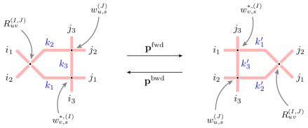
Figure 11. A graphical representation of the Yang-Baxter Equation (6.6) and its bijectivization.

For simplicity we do not include the external occupation numbers $i_{1},i_{2},i_{3},j_{1},j_{2},j_{3}\in\mathbb{Z}_{\geq 0}$ in the notation $\mathbf{p}^{\mathrm{fwd}}$ and $\mathbf{p}^{\mathrm{bwd}}$. Let us extend the definition of $\mathbf{p}^{\mathrm{fwd}},\mathbf{p}^{\mathrm{bwd}}$ by setting

$$\mathbf{p}^{\mathrm{fwd}}\Bigg{(}\leavevmode\hbox to56.17pt{\vbox to42.2pt{\text{[drawing]}}},\leavevmode\hbox to56.17pt{\vbox to48.67pt{\text{[drawing]}}}\Bigg{)}=0, i_{2} i_{1} i_{3} j_{1} j_{2} j_{3} k_{1} k_{2} k_{3} i_{1}^{\prime} i_{2}^{\prime} i_{3}^{\prime} j_{1}^{\prime} j_{2}^{\prime} j_{3}^{\prime} k_{1}^{\prime} k_{2}^{\prime} k_{3}^{\prime} i_{2} i_{1} i_{3} j_{1} j_{2} j_{3} k_{1} k_{2} k_{3} i_{1}^{\prime} i_{2}^{\prime} i_{3}^{\prime} j_{1}^{\prime} j_{2}^{\prime} j_{3}^{\prime} k_{1}^{\prime} k_{2}^{\prime} k_{3}^{\prime}$$ (6.7)

whenever $(i_{1},i_{2},i_{3},j_{1},j_{2},j_{3})\neq(i_{1}^{\prime},i_{2}^{\prime},i_{3}^{\prime},j_{1}^{\prime},j_{2}^{\prime},j_{3}^{\prime})$, and analogously for $\mathbf{p}^{\mathrm{bwd}}$. Thus, we will view $\mathbf{p}^{\mathrm{fwd}}$ as the probability of a Markov transition of pushing the cross through a column of two vertices in the right direction, and similarly $\mathbf{p}^{\mathrm{bwd}}$ corresponds to pushing the cross to the left. These transitions do not change the external occupation numbers $(i_{1},i_{2},i_{3},j_{1},j_{2},j_{3})$, but $\mathbf{p}^{\mathrm{fwd}}$ changes fixed occupation numbers $(k_{1},k_{2},k_{3})$ into random $(k_{1}^{\prime},k_{2}^{\prime},k_{3}^{\prime})$, and similarly $\mathbf{p}^{\mathrm{bwd}}$ maps $(k_{1}^{\prime},k_{2}^{\prime},k_{3}^{\prime})$ into random $(k_{1},k_{2},k_{3})$.

6.3. Dragging a cross through multiple columns. Yang-Baxter fields

We now want to bring our discussion a step forward and push the cross through multiple columns of vertices, from the leftmost one to the right (and vice versa), sequentially utilizing the transition probabilities $\mathbf{p}^{\mathrm{fwd}}$ and $\mathbf{p}^{\mathrm{bwd}}$ associated with the vertex weights $w^{(J)}_{u,s}$, $w^{*,(I)}_{v,s}$, and $R^{(I,J)}_{uv}$ which are nonnegative in one of the cases given in Figure 10.

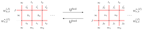
Figure 12. Graphical representation of a transition between two-row path configurations.

We consider the lattice composed of two infinite rows, that is, the vertices are indexed by the lattice $\mathbb{Z}_{\geq 0}\times\{1,2\}$. The rows carry vertex weights $w^{(J)}_{u,s}$ and $w^{*,(I)}_{v,s}$ (see Figure 12 for an illustration). As boundary conditions for the paths flowing through the lattice we take:

• infinitely many paths flow in the vertical direction in the 0-th column; • at the 0-th column no paths enter from the left into the vertex carrying the weight $$w^{*,(I)}_{v,s} J w^{(J)}_{u,s}$$, while paths enter from the left into the vertex in the 0-th column carrying the weight ; • paths do not stay horizontal forever, that is, at the far right the path configuration must be empty. (6.8)

Remark 6.5.

Under the sqW or scaled geometric specializations treating $q^{J}$ as an independent variable, the term “$J$ paths” in (6.8) should be understood formally and all the vertex weights should undergo these specializations together (see Remark 7.5 below for a detailed explanation of this procedure). In the rest of the present section we continue to employ the unified notation for all the cases.

The numbers of vertical arrows in the path configurations in Figure 12 are encoded by triples of Young diagrams $\lambda,\varkappa,\mu$ (left) and $\lambda,\nu,\mu$ (right), as the horizontal edges’ occupation numbers are then uniquely determined by the arrow preservation. In detail, we have

$$\lambda=1^{l_{1}}2^{l_{2}}\dots,\qquad\mu=1^{m_{1}}2^{m_{2}}\dots,\qquad\varkappa=1^{k_{1}}2^{k_{2}},\dots,\qquad\nu=1^{n_{1}}2^{n_{2}}\dots.$$ (6.9)

Let us record the corresponding horizontal occupation numbers by sequences $\{i_{h},i_{h}^{\prime}\}_{h\geq 0}$ (for $\lambda,\varkappa,\mu$) and $\{j_{h},j_{h}^{\prime}\}_{h\geq 0}$ (for $\lambda,\nu,\mu$).

Definition 6.6 (Markov operators on Young diagrams).

With the above notation, we define the Markov operators $\mathsf{U}^{\mathrm{fwd}}$ and $\mathsf{U}^{\mathrm{bwd}}$ as follows. For $\mathsf{U}^{\mathrm{fwd}}$, attach the cross vertex to the leftmost column in the configuration encoded by $(\lambda,\varkappa,\mu)$, and drag the cross all the way to the right using the transition probabilities $\mathbf{p}^{\mathrm{fwd}}$. An intermediate step is displayed in Figure 13. The definition of $\mathsf{U}^{\mathrm{bwd}}$ involves dragging the cross to the left using the transition probabilities $\mathbf{p}^{\mathrm{bwd}}$, and starting from the empty cross vertex far to the right. In detail,

$$\mathsf{U}^{\mathrm{fwd}}(\varkappa\to\nu\mid\lambda,\mu)=\prod_{h=0}^{\infty}\mathbf{p}^{\mathrm{fwd}}\Bigg{(}\leavevmode\hbox to58.93pt{\vbox to46.91pt{\text{[drawing]}}},\leavevmode\hbox to58.93pt{\vbox to52.6pt{\text{[drawing]}}}\Bigg{)}; j_{h-1} j_{h-1}^{\prime} m_{h} i_{h} i_{h}^{\prime} l_{h} i_{h-1} i_{h-1}^{\prime} k_{h} j_{h-1}^{\prime} j_{h-1} m_{h} i_{h} i_{h}^{\prime} l_{h} j_{h} j_{h}^{\prime} n_{h} j_{h-1} j_{h-1}^{\prime} m_{h} i_{h} i_{h}^{\prime} l_{h} i_{h-1} i_{h-1}^{\prime} k_{h} j_{h-1}^{\prime} j_{h-1} m_{h} i_{h} i_{h}^{\prime} l_{h} j_{h} j_{h}^{\prime} n_{h}$$ (6.10)

$$\mathsf{U}^{\mathrm{bwd}}(\nu\to\varkappa\mid\lambda,\mu)=\prod_{h=0}^{\infty}\mathbf{p}^{\mathrm{bwd}}\Bigg{(}\leavevmode\hbox to58.93pt{\vbox to52.6pt{\text{[drawing]}}},\leavevmode\hbox to58.93pt{\vbox to46.91pt{\text{[drawing]}}}\Bigg{)}, j_{h-1}^{\prime} j_{h-1} m_{h} i_{h} i_{h}^{\prime} l_{h} j_{h} j_{h}^{\prime} k_{h} j_{h-1} j_{h-1}^{\prime} m_{h} i_{h} i_{h}^{\prime} l_{h} i_{h-1} i_{h-1}^{\prime} n_{h} j_{h-1}^{\prime} j_{h-1} m_{h} i_{h} i_{h}^{\prime} l_{h} j_{h} j_{h}^{\prime} k_{h} j_{h-1} j_{h-1}^{\prime} m_{h} i_{h} i_{h}^{\prime} l_{h} i_{h-1} i_{h-1}^{\prime} n_{h}$$ (6.11)

where $j_{-1}=J$, $j_{-1}^{\prime}=0$, and $i_{h}=i_{h}^{\prime}=0$ for all sufficiently large $h$. All terms $\mathbf{p}^{\mathrm{fwd}}$ and $\mathbf{p}^{\mathrm{bwd}}$ in the infinite products (6.10), (6.11) belong to $[0,1]$.

Figure 13. As the cross moves to the right, it randomly updates values of vertical occupation numbers $k_{h}$ to $n_{h}$ (in $\mathsf{U}^{\mathrm{fwd}}$). Horizontal occupation numbers are updated accordingly.

Because the definition of $\mathsf{U}^{\mathrm{fwd}}$ and $\mathsf{U}^{\mathrm{bwd}}$ involves Yang-Baxter equations with infinitely many paths, we have to make sure that the corresponding infinite sums converge. Recall the sets $\mathsf{Adm}(\rho,\rho^{*})$ from Definition 5.2 and the restrictions on parameters in Figure 10 leading to positive specializations.

Proposition 6.7.

For each of the 9 pairs of specializations $(\rho,\rho^{*})$ from Figure 10 (when $\rho$ and $\rho^{*}$ correspond to $w_{u,s}^{(J)}$ and $w_{v,s}^{*,(I)}$, respectively) when the parameters belong to $\mathsf{Adm}(\rho,\rho^{*})$, one can choose bijectivizations $\mathbf{p}^{\mathrm{fwd}}$ and $\mathbf{p}^{\mathrm{bwd}}$ such that the Markov operators $\mathsf{U}^{\mathrm{fwd}}$ and $\mathsf{U}^{\mathrm{bwd}}$ are well-defined by the infinite products (6.10) and (6.11). That is,

$$\sum_{\nu}\mathsf{U}^{\mathrm{fwd}}(\varkappa\to\nu\mid\lambda,\mu)=1,\qquad\sum_{\varkappa}\mathsf{U}^{\mathrm{bwd}}(\nu\to\varkappa\mid\lambda,\mu)=1,$$

where the sums are taken over all path configurations as in Figure 12 (with $\varkappa$ and $\nu$ encoding the left and right pictures, respectively) with the boundary conditions (6.8).

This implies in particular that the Markov operator $\mathsf{U}^{\mathrm{fwd}}$ does not produce path configurations with infinitely long horizontal paths on the right or infinitely many vertical paths in any column except the leftmost one.

Proof of Proposition 6.7.

Step 1. The backward transition probabilities $\mathsf{U}^{\mathrm{bwd}}(\nu\to\varkappa\mid\lambda,\mu)$ sum to one over $\varkappa$ because for fixed $\lambda,\nu,\mu$ the number of possible configurations $\varkappa$ is finite in all the cases considered in Sections 3.5, 3.7 and 3.8. Therefore, only finitely many factors in the products (6.11) differ from $1$. As the individual pieces $\mathbf{p}^{\mathrm{bwd}}$ sum to one over all possible outcomes, we see that the backward operator $\mathsf{U}^{\mathrm{bwd}}$ is well-defined.

Step 2. We will now show that there exists a bijectivization $\mathbf{p}^{\mathrm{fwd}}$ such that for all $j\geq 1$ we have

$$\mathbf{p}^{\mathrm{fwd}}\Bigg{(}\leavevmode\hbox to51.64pt{\vbox to39.34pt{\text{[drawing]}}},\leavevmode\hbox to51.64pt{\vbox to45.03pt{\text{[drawing]}}}\Bigg{)}<1. j j j j j j j j j j j j$$ (6.12)

This condition ensures that all probability mass is concentrated on triples $(\lambda,\nu,\mu)$ with boundary conditions (6.8), and no positive probability is assigned under $\mathsf{U}^{\mathrm{fwd}}$ to configurations with infinitely long horizontal paths. Indeed, if there are $j$ paths escaping to the right past $\max(\mu_{1},\lambda_{1})$, then due to (6.12) after a random geometric number of cross draggings to the right there will remain $j-1$ paths, and so on until the configuration of paths far to the right becomes empty.

The Yang-Baxter equation with the boundary conditions corresponding to (6.12) has the form

$$\sum_{a=0}^{j}\mathrm{weight}\Bigg{(}\leavevmode\hbox to51.64pt{\vbox to39.34pt{\text{[drawing]}}}\Bigg{)}=\sum_{b=0}^{j}\mathrm{weight}\Bigg{(}\leavevmode\hbox to51.64pt{\vbox to45.03pt{\text{[drawing]}}}\Bigg{)}. j j a a a j j b j-b j-b j j a a a j j b j-b j-b$$ (6.13)

It is possible to choose a bijectivization satisfying (6.12) if at least one term in the right-hand side of (6.13) corresponding to some $b>0$ does not vanish. These terms are given by

$$\mathrm{weight}\Bigg{(}\leavevmode\hbox to51.64pt{\vbox to45.03pt{\text{[drawing]}}}\Bigg{)}=w_{u,s}^{(J)}(0,j;b,j-b)w_{v,s}^{*,(I)}(b,j;0,j-b)R_{uv}^{(I,J)}(j-b,j-b;0,0). j j b j-b j-b j j b j-b j-b$$

We now consider the cases of Figure 10 separately. In the cases involving the sHL specialization, the only allowed positive $j$ is $j=1$, and the positivity of the term corresponding to $b=1$ can be checked by writing down all possible cases:

$$\begin{array}[]{rclrcl}\mathrm{sHL/sHL}&:&\dfrac{(1-q)(1-s^{2})}{(1-su)(1-sv)},\\ \mathrm{sHL/sqW}&:&\dfrac{1-q}{1-su},&\qquad\qquad\mathrm{sqW/sHL}&:&\dfrac{1-q}{1-sv},\rule{0.0pt}{25.0pt}\\ \mathrm{sHL/sg}&:&\dfrac{(1-q)(1-s^{2})}{1-su},&\qquad\qquad\mathrm{sg/sHL}&:&\dfrac{(1-q)(1-s^{2})}{1-sv}.\rule{0.0pt}{25.0pt}\end{array}$$

All these expressions are positive under the positivity conditions from Figure 10.

Next, in the sqW/sqW, case, the number of paths $j\geq 1$ can be arbitrary, but the product $W_{x,s}(0,j;b,j-b)W^{*}_{y,s}(b,j;0,j-b)$ vanishes unless $b=j$, and for $b=j$ it is positive. The same is true for the sqW/sg and sg/sqW cases. Finally, in the sg/sg case all factors of the form $\widetilde{w}_{\alpha,s}(0,j;b,j-b)\widetilde{w}^{*}_{\beta,s}(b,j;0,j-b)R^{(\mathrm{sg,sg})}_{\alpha,\beta}(j-b,j-b;0,0)$ are strictly positive.

Step 3. Now let us check that after dragging the cross through the leftmost column containing infinitely many vertical paths, the probability to get infinitely many horizontal paths is zero. Clearly, infinitely many horizontal paths might occur only if neither of the specializations $\rho,\rho^{*}$ is sHL. Overall, we need to show that

$$\sum_{j_{0},j_{0}^{\prime}}\mathbf{p}^{\mathrm{fwd}}\Bigg{(}\leavevmode\hbox to55.67pt{\vbox to43.65pt{\text{[drawing]}}},\leavevmode\hbox to55.67pt{\vbox to49.34pt{\text{[drawing]}}}\Bigg{)}=1. J \infty i_{0} i_{0}^{\prime} \infty J \infty J \infty i_{0} i_{0}^{\prime} \infty j_{0} j_{0}^{\prime} \infty J \infty i_{0} i_{0}^{\prime} \infty J \infty J \infty i_{0} i_{0}^{\prime} \infty j_{0} j_{0}^{\prime} \infty$$ (6.14)

Considering the corresponding Yang-Baxter equation, we see that its left-hand side converges thanks to Proposition A.5, because the weights of the other two vertices do not depend on the input from the left (cf. (3.14), (A.16)). The right-hand side of this Yang-Baxter equation contains terms of the form $w^{*,(I)}_{v,s}(\infty,0;\infty,j_{0}^{\prime})\,w^{(J)}_{u,s}(\infty,J;\infty,j_{0})\,R^{(I,J)}_{uv}(j_{0},j_{0}^{\prime};i_{0}^{\prime},i_{0})$. In the sqW/sqW, sqW/sg, and sg/sg cases, the cross vertex weights (A.14), (A.19), and (A.20) are bounded for fixed $i_{0},i_{0}^{\prime}$. The contribution from the other two vertices regulating the convergence of the right-hand side of the Yang-Baxter equation amounts to $(\xi\theta)^{j_{0}}$, $(\xi\beta)^{j_{0}}$, or $(\alpha\beta)^{j_{0}}$, respectively. The conditions $\mathsf{Adm}(\rho,\rho^{*})$ in these cases precisely mean that the products of spectral parameters are less than one, so the series converge. One then can choose a bijectivization such that (6.14) holds. This completes the proof. ∎

Definition 6.6 and Proposition 6.7 thus produce “natural” Markov operators $\mathsf{U}^{\mathrm{fwd}}$ and $\mathsf{U}^{\mathrm{bwd}}$ associated with each of our skew Cauchy structures. Denote by $\mathfrak{F}_{\lambda/\varkappa}(\rho)$ and $\mathfrak{G}_{\mu/\varkappa}(\rho^{*})$ the partition functions of the one-row configurations in the top and the bottom rows, respectively, in Figure 12, left. By their very construction through local bijectivizations, these Markov operators satisfy the reversibility condition for all $\lambda,\mu,\varkappa,\nu$:

$$\mathsf{U}^{\mathrm{fwd}}(\varkappa\to\nu\mid\lambda,\mu)\cdot\Pi(\rho;\rho^{*})\mathfrak{F}_{\lambda/\varkappa}(\rho)\mathfrak{G}_{\mu/\varkappa}(\rho^{*})=\mathsf{U}^{\mathrm{bwd}}(\nu\to\varkappa\mid\lambda,\mu)\cdot\mathfrak{F}_{\nu/\mu}(\rho)\mathfrak{G}_{\nu/\lambda}(\rho^{*}).$$

Here $\Pi(\rho;\rho^{*})$ is defined in Theorem 5.3, which can be viewed as the properly specialized term $\dfrac{(uvq^{I};q)_{\infty}(uvq^{J};q)_{\infty}}{(uv;q)_{\infty}(uvq^{I+J};q)_{\infty}}$ from the right-hand side of the Cauchy equation (5.3). Moreover, this quantity is also identified with the weight of the cross vertex $(J,0;J,0)$ attached to the configuration in Figure 12, left, before dragging the cross to the right (see Proposition A.5 for the last equality).

Thus, we have constructed Yang-Baxter random fields of Young diagrams, which are illustrated in Figure 14. Before discussing concrete details in each of the different cases in Section 7 below, in the next Section 6.4 we look at scalar marginals of our random fields.

Figure 14. Yang-Baxter field and forward and backward Markov transition operators $\mathsf{U}^{\mathrm{fwd}}$ and $\mathsf{U}^{\mathrm{bwd}}$.

6.4. Marginals

We now apply the discussion of Section 2.5 to the Yang-Baxter fields constructed above. Due to the sequential left-to-right update rule in the definition of $\mathsf{U}^{\mathrm{fwd}}$, there is a number of marginals $\mathsf{h}$ to which our fields $\boldsymbol{\lambda}$ are adapted to.

Fix $h\geq 2$. For a Young diagram $\eta=1^{n_{1}}2^{n_{2}}\ldots$ introduce the decomposition

$$\eta=(\eta^{[<h]},\eta^{[\geq h]}),\qquad\eta^{[<h]}=1^{n_{1}}\ldots(h-1)^{n_{h-1}},\qquad\eta^{[\geq h]}=h^{n_{h}}(h+1)^{n_{h+1}}\ldots,$$ (6.15)

where $\eta^{[<h]}$ and $\eta^{[\geq h]}$ are two new Young diagrams.

Proposition 6.8.

Let $\mathsf{h}$ be either of the following functions on the set of Young diagrams:

• $\mathsf{h}(\eta)=\ell(\eta)$;

• $\mathsf{h}(\eta)=\bigl{(}\eta^{[<h]},\ell(\eta^{[\geq h]})\bigr{)}$ for some $h\geq 2$.

Then each of the Yang-Baxter fields $\boldsymbol{\lambda}$ constructed in Section 6.3 is adapted to $\mathsf{h}$ in the sense of Section 2.5.

Proof.

Let first $h>1$. From the definition of $\mathsf{U}^{\mathrm{fwd}}$ (6.10) we see that the random moves of the first $h$ columns of vertices are independent of those taking place in columns to their right. Therefore, summing $\mathsf{U}^{\mathrm{fwd}}(\varkappa\to\nu\mid\lambda,\mu)$ over $\nu$ with fixed $\nu^{[<h]}$ and $\ell(\nu)$, we see that the result is independent of $\varkappa^{[\geq h]},\nu^{[\geq h]},\lambda^{[\geq h]},\mu^{[\geq h]}$. The quantities $\ell(\varkappa^{[\geq h]}),\ell(\nu^{[\geq h]}),\ell(\lambda^{[\geq h]}),\ell(\mu^{[\geq h]})$ encode the numbers of paths flowing through the horizontal edges between columns $h$ and $h+1$ (recall that $\lambda$ and $\mu$ are fixed throughout the random update). This proves the statement for $\mathsf{h}(\eta)=\bigl{(}\eta^{[<h]},\ell(\eta^{[\geq h]})\bigr{)}$.

When $h=0$, that is, when we consider the marginal move at the leftmost column, we only record the number of arrows entering the lattice (evolving in a marginally Markovian manner), which are simply the lengths of $\varkappa,\nu,\lambda,\mu$. This establishes the remaining case $\mathsf{h}(\eta)=\ell(\eta)$. ∎

Let us denote the transition probabilities of the marginal processes afforded by Proposition 6.8 by $\mathsf{U}^{[0]}$ and $\mathsf{U}^{[<h]}$, respectively.

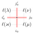
Figure 15. Evolution of the lengths of Young diagrams under $\mathsf{U}^{[0]}$. Moving around the vertex along dotted lines changes the length of a Young diagram by the occupation number of the edge we cross, cf. (6.16).

We will mostly be interested in the simplest case $\mathsf{U}^{[0]}$. One readily sees that the action of the Markov operator $\mathsf{U}^{[0]}$ is encoded as the evolution of the horizontal occupation numbers $\{i_{0},i_{0}^{\prime}\}\to\{j_{0},j_{0}^{\prime}\}$, where

$$i_{0}=\ell(\mu)-\ell(\varkappa),\quad i_{0}^{\prime}=\ell(\lambda)-\ell(\varkappa);\qquad j_{0}=\ell(\nu)-\ell(\mu),\quad j_{0}^{\prime}=\ell(\nu)-\ell(\lambda)$$ (6.16)

(see Figures 12 and 15 for an illustration). Therefore, let us use the notation $\mathsf{U}^{[0]}(i_{0},i_{0}^{\prime};j_{0},j_{0}^{\prime})$ for these transition probabilities. We have

$$\mathsf{U}^{[0]}(i_{0},i_{0}^{\prime};j_{0},j_{0}^{\prime})=\mathbf{p}^{\mathrm{fwd}}\Bigg{(}\leavevmode\hbox to55.67pt{\vbox to43.65pt{\text{[drawing]}}},\leavevmode\hbox to55.67pt{\vbox to49.34pt{\text{[drawing]}}}\Bigg{)}. J \infty i_{0} i_{0}^{\prime} \infty J \infty J \infty i_{0} i_{0}^{\prime} \infty j_{0} j_{0}^{\prime} \infty J \infty i_{0} i_{0}^{\prime} \infty J \infty J \infty i_{0} i_{0}^{\prime} \infty j_{0} j_{0}^{\prime} \infty$$

This probability is determined uniquely because the right-hand side of the Yang-Baxter equation contains a single summand corresponding to the state $(J,0;J,0)$ of the cross vertex (this is enforced by our arrow preservation conventions). Thus, by Example 6.3, this probability can be written as a ratio of weights of 3-vertex configurations as follows:

$$\mathsf{U}^{[0]}(i_{0},i_{0}^{\prime};j_{0}^{\prime},j_{0})=\frac{w^{*,(I)}_{v,s}(\infty,0;\infty,j_{0}^{\prime})\,w^{(J)}_{u,s}(\infty,J;\infty,j_{0})\,R^{(I,J)}_{uv}(j_{0},j_{0}^{\prime};i_{0}^{\prime},i_{0})}{R^{(I,J)}_{uv}(J,0;J,0)\,w^{*,(I)}_{v,s}(\infty,0;\infty,i_{0})\,w^{(J)}_{u,s}(\infty,J;\infty,i_{0}^{\prime})}.$$ (6.17)

This expression vanishes unless $i_{0}+j_{0}=i_{0}^{\prime}+j_{0}^{\prime}$. The quantity $R^{(I,J)}_{uv}(J,0;J,0)$ in the denominator has an explicit form (A.10).

Formula (6.17) also appeared in the recent work [ABB18] under the name of “stochasticization” of the solution of a Yang-Baxter equation. In this paper we explicitly link stochasticizations to known stochastic vertex models (including the stochastic six vertex model [GS92], [BCG16], the higher spin stochastic six vertex model [Bor17], [CP16], [BP18], and a pushing system introduced recently in [CMP18]), and show the existence of the corresponding full Yang-Baxter fields. The latter further connects observables of stochastic vertex models to probability distributions based on spin Hall-Littlewood and spin $q$-Whittaker functions.

The other marginals $\mathsf{U}^{[<h]}$, $h\geq 2$, lead to multilayer versions of stochastic vertex models. A multilayer version of the stochastic six vertex model was introduced recently in [BM18] (and another such system was constructed in [BP17] using Yang-Baxter fields). Multilayer systems are much less explicit and are not determined uniquely due to the non-uniqueness of $\mathsf{U}^{\mathrm{fwd}}$. They deserve their own study, and in the present paper we mostly focus on $\mathsf{U}^{[0]}$.

7. Three Yang-Baxter fields

7.1. Preliminaries

In this section we present detailed descriptions of the Yang-Baxter fields associated with the skew Cauchy structures defined in Section 3 (with the step or scaled geometric boundary conditions). We also discuss the scalar marginals $\mathsf{h}(\lambda^{(x,y)})=\ell(\lambda^{(x,y)})$ of these Yang-Baxter fields. Let us first make two general remarks.

Remark 7.1.

The definitions of the Yang-Baxter fields in this section involve non-unique local bijectivizations, and so these fields are not defined in a unique way. However, all our statements hold for any such choice of a bijectivization. Moreover, the distributions of the scalar marginals $\ell(\lambda^{(x,y)})$ do not depend on the choice of a bijectivization. Thus, for shortness we will use the term “the Yang-Baxter field” to refer to any random field of Young diagrams coming from bijectivizations of the Yang-Baxter equations.

Remark 7.2 (On stationary boundary conditions).

The (two-sided) scaled geometric boundary conditions for our Yang-Baxter fields match (in scalar marginals viewed as stochastic particle systems on the line) to initial conditions composed of two half-stationary pieces (of possibly different densities) glued together at the origin. For example, for the stochastic six vertex model (as well as for ASEP and TASEP) on the line, the stationary initial data is the product Bernoulli one, and so the two-sided stationary initial condition is composed of two product Bernoulli configurations of arbitrary densities on the half-lines. When the densities match and the systems’ parameters are homogeneous (i.e., independent of $x,y$), this initial data is indeed stationary under the stochastic evolution on the line.

However, one can check that for the full Yang-Baxter fields, the scaled geometric boundary conditions do not contain a subfamily of boundary conditions remaining stationary under the evolution of the full Young diagrams. Therefore, we distinguish the terms “scaled geometric” and “two-sided stationary” boundary conditions — the former refers to full Yang-Baxter fields, and the latter — to stochastic particle systems arising as one-dimensional marginals.

7.2. The sHL/sHL Yang-Baxter field and the stochastic six vertex model

We first discuss the simplest case, the sHL/sHL skew Cauchy structure, and relate the corresponding field to the stochastic six vertex model of [GS92], [BCG16]. The case of step boundary conditions essentially parallels [BP17] (without the dynamic modification of the six vertex model because here we work with the stable sHL functions instead of the non-stable ones). Formulas for observables and asymptotics in the six vertex model with two-sided stationary boundary conditions were studied in [Agg18], but its connection to symmetric functions is new.

7.2.1. Step boundary conditions

The sHL/sHL case is obtained by setting $I=J=1$ in Section 6, and the field depends on the parameters $q\in(0,1)$, $s\in(-1,0)$, and $u_{y},v_{x}\in[0,1)$, $x,y\in\mathbb{Z}_{\geq 1}$. The Yang-Baxter equation corresponding to this skew Cauchy structure is now (A.2). The reversibility property of backward and forward operators takes the following form:

Proposition 7.3.

For any four Young diagrams $\mu,\varkappa,\lambda,\nu$ we have

$$\frac{1-quv}{1-uv}\,\mathsf{U}_{\mathrm{sHL}(u),\mathrm{sHL}(v)}^{\mathrm{fwd}}(\varkappa\to\nu\mid\lambda,\mu)\,\mathsf{F}_{\lambda/\varkappa}(u)\,\mathsf{F}^{*}_{\mu/\varkappa}(v)\\ =\mathsf{U}_{\mathrm{sHL}(u),\mathrm{sHL}(v)}^{\mathrm{bwd}}(\nu\to\varkappa\mid\lambda,\mu)\,\mathsf{F}^{*}_{\nu/\lambda}(v)\,\mathsf{F}_{\nu/\mu}(u).$$ (7.1)

Summing (7.1) over both $\varkappa$ and $\nu$, we obtain the skew Cauchy identity for the stable sHL functions (Theorem 3.4).

Proof.

The product $\mathsf{F}_{\lambda/\varkappa}(u)\mathsf{F}^{*}_{\mu/\varkappa}(v)$ is the weight of a configuration $\mu\succ\varkappa\prec\lambda$ in a vertex model obtained attaching a $w_{u,s}$-weighted row of vertices on top of a $w^{*}_{v,s}$-weighted row of vertices. The leftmost column is occupied by infinitely many paths. The factor $(1-quv)/(1-uv)$ is the $R_{uv}$ weight of a cross attached at the left of the lattice. Now we employ the definition of $\mathsf{U}^{\mathrm{fwd}}_{\mathrm{sHL}(u),\mathrm{sHL}(v)}$ and drag the cross all the way to the right, replacing $\varkappa$ by the random $\nu$. This procedure, along with the local reversibility condition of the bijectivization leaves us with the right-hand side of the desired identity (7.1). ∎

The step boundary conditions are $\lambda^{(0,y)}=\lambda^{(x,0)}=0^{\infty}=\varnothing$, and using the forward transition operators $\mathsf{U}^{\mathrm{fwd}}_{\mathrm{sHL}(u_{y}),\mathrm{sHL}(v_{x})}$ as described in Section 2.4, we generate the the sHL/sHL Yang-Baxter field $\boldsymbol{\lambda}=\{\lambda^{(x,y)}:x,y\in\mathbb{Z}_{\geq 0}\}$. Its distributions are related to the sHL functions:

Proposition 7.4.

The single-point distributions in the sHL/sHL Yang-Baxter field with the step boundary conditions have the form

$$\mathrm{Prob}\bigl{(}\lambda^{(x,y)}=\nu\bigr{)}=\prod_{\begin{subarray}{c}1\leq i\leq x\\ 1\leq j\leq y\end{subarray}}\frac{1-u_{j}v_{i}}{1-qu_{j}v_{i}}\,\mathsf{F}_{\nu}(u_{1},\dots,u_{y})\,\mathsf{F}^{*}_{\nu}(v_{1},\dots,v_{x}),$$

where $\nu$ is an arbitrary fixed Young diagram. Moreover, joint distributions in this field along down-right paths are expressed through products of skew sHL functions as in Proposition 2.9.

7.2.2. Scaled geometric boundary conditions

Fix additional parameters $\alpha,\beta\in[0,-s^{-1}]$, and consider specializations $\rho^{\mathrm{v}}_{i}$, $\rho^{\mathrm{h}}_{i}$, $i=-1,0,1,\ldots$:

$$\rho^{\mathrm{v}}_{-1}=\mathrm{sg}(\alpha),\quad\rho^{\mathrm{h}}_{-1}=\mathrm{sg}(\beta),\qquad\rho^{\mathrm{v}}_{y}=\mathrm{sHL}(u_{y}),\quad\rho^{\mathrm{h}}_{x}=\mathrm{sHL}(v_{x}),\quad x,y\geq 0.$$

Let $\boldsymbol{\eta}$ be the Yang-Baxter field on the lattice $\mathbb{Z}_{\geq-1}\times\mathbb{Z}_{\geq-1}$ generated by the Markov transition operators $\mathsf{U}_{\rho^{\mathrm{v}}_{y},\rho^{\mathrm{h}}_{x}}^{\mathrm{fwd}}$.

Remark 7.5.

In defining forward transition operators for scaled geometric (or later spin $q$-Whittaker) specializations by dragging the cross vertex $(J,0;J,0)$ to the right (as explained in Section 6.3) we encounter the issue that the number of paths $J$ should be specialized via $q^{J}=1/\epsilon$, $\epsilon\to 0$, and so the vertex $(J,0;J,0)$ no longer makes direct sense. However, by Proposition A.5 we explicitly know the weight of $(J,0;J,0)$, which is equal to

$$R_{uv}^{(I,J)}(J,0;J,0)=\frac{(uvq^{I};q)_{\infty}(uvq^{J};q)_{\infty}}{(uv;q)_{\infty}(uvq^{I+J};q)_{\infty}}.$$

This expression can readily be taken to the scaled geometric or the spin $q$-Whittaker specialization (cf. Figure 10 for explicit forms of the specializations). Therefore, in choosing the bijectivization of the Yang-Baxter equation in the leftmost column we can still appeal to Example 6.3, and conclude that the bijectivization is unique.

Restricting the field $\boldsymbol{\eta}$ to the nonnegative quadrant, denote $\boldsymbol{\lambda}=\boldsymbol{\eta}|_{{}_{\mathbb{Z}_{\geq 0}\times\mathbb{Z}_{\geq 0}}}$. We call $\boldsymbol{\lambda}$ the sHL/sHL Yang-Baxter field with $(\alpha,\beta)$-scaled geometric boundary conditions.

Proposition 7.6.

The single-point distributions in the sHL/sHL Yang-Baxter field with the $(\alpha,\beta)$-scaled geometric boundary conditions are given by

$$\mathrm{Prob}\{\lambda^{(x,y)}=\nu\}=\frac{(\alpha\beta;q)_{\infty}}{\prod\limits_{j=1}^{y}(1+u_{j}\beta)\prod\limits_{i=1}^{x}(1+v_{i}\alpha)}\,\prod_{\begin{subarray}{c}1\leq i\leq x\\ 1\leq j\leq y\end{subarray}}\frac{1-u_{j}v_{i}}{1-qu_{j}v_{i}}\,\mathsf{F}_{\nu}(u_{1},\dots,u_{y};\widetilde{\alpha})\mathsf{F}^{*}_{\nu}(v_{1},\dots,v_{x};\widetilde{\beta}).$$

Joint distributions in this field along down-right paths are expressed through products of skew functions similarly to Proposition 2.9.

7.2.3. Stochastic six vertex model

We now turn to the scalar Markov marginal $\mathsf{h}(\lambda^{(x,y)})=\ell(\lambda^{(x,y)})$ of the sHL/sHL Yang-Baxter field, and match it to the stochastic six vertex model.

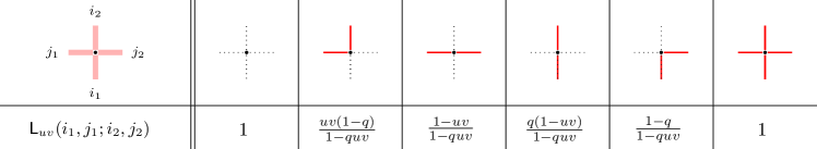
Figure 16. The vertex weights $\mathsf{L}_{uv}(i_{1},j_{1};i_{2},j_{2})$ in the stochastic six vertex model. This parametrization of the vertex weights follows, e.g., [BM18].

Definition 7.7 ([GS92], [BCG16]).

Fix $q\in(0,1)$ and $u_{y},v_{x}$ such that $0<u_{y}v_{x}<1$ for all $x,y\in\mathbb{Z}_{\geq 1}$. Consider the stochastic vertex weights $\mathsf{L}_{u_{y}v_{x}}$ given in Figure 16. Let us also fix the boundary conditions $B^{\mathrm{h}}=\{b^{\mathrm{h}}_{1},b^{\mathrm{h}}_{2},\dots\}$ and $B^{\mathrm{v}}=\{b^{\mathrm{v}}_{1},b^{\mathrm{v}}_{2},\dots\}$, where $b_{i}^{\mathrm{h}},b_{j}^{\mathrm{v}}\in\left\{0,1\right\}$. The (inhomogeneous) stochastic six vertex model with these boundary conditions is the (unique) probability measure on the set of up-right directed paths on the lattice $\mathbb{Z}_{\geq 0}\times\mathbb{Z}_{\geq 0}$ (with at most one path per vertical or horizontal edge) satisfying:

• Each vertex $(0,y)$ at the vertical boundary $\{(0,y^{\prime}):y^{\prime}\geq 1\}$ emanates a path initially pointing to the right if $b^{\mathrm{v}}_{y}=1$;

• Each vertex $(x,0)$ at the horizontal boundary $\{(x^{\prime},0):x^{\prime}\geq 1\}$ emanates a path initially pointing upward if $b^{\mathrm{h}}_{x}=1$;

• For each $(x,y)$, conditioned to the path configuration at all vertices $(x^{\prime},y^{\prime})$ such that $x^{\prime}+y^{\prime}<x+y$, the probability of a vertex configuration $(i_{1},j_{1};i_{2},j_{2})$ at $(x,y)$ is given by $\mathsf{L}_{u_{y}v_{x}}(i_{1},j_{1};i_{2},j_{2})$. Moreover, the random choices made at diagonally adjacent vertices $\ldots,(x-1,y+1),(x,y),(x+1,y-1),\ldots$ are independent under the same condition.

In particular, the step boundary conditions correspond to

$$b^{\mathrm{h}}_{x}=0\qquad\text{and}\qquad b^{\mathrm{v}}_{y}=1,\qquad\text{for all }x,y\geq 1.$$ (7.2)

Path configurations in the six vertex model with the step boundary conditions are conveniently encoded by a height function. Namely, let $\mathfrak{h}^{\mathrm{6V}}(x,y)$ denote the number of paths which pass weakly to the right of the vertex $(x,y)$. See Figure 17, right, for an illustration. The next theorem is a version of [BP17, Proposition 7.3] adapted to our boundary conditions in the Yang-Baxter field.

Let $\boldsymbol{\lambda}=\{\lambda^{(x,y)}\}$ be the sHL/sHL Yang-Baxter field with the step boundary conditions, and $\mathfrak{h}^{\mathrm{6V}}(x,y)$ be the six vertex height function with the step boundary conditions (7.2).

Theorem 7.8.

The two random fields $\{y-\ell(\lambda^{(x,y)}):x,y\in\mathbb{Z}_{\geq 0}\}$ and $\{\mathfrak{h}^{\mathrm{6V}}(x+1,y):x,y\in\mathbb{Z}_{\geq 0}\}$ are equal in distribution.

Proof.

Recall that the Markov evolution of this scalar marginal $\ell(\lambda^{(x,y)})$ corresponds to the quantities $\mathsf{U}^{[0]}(i_{0},i_{0}^{\prime};j_{0}^{\prime},j_{0})$ (6.17) with $I=J=1$ and $i_{0},i_{0}^{\prime},j_{0},j_{0}^{\prime}\in\left\{0,1\right\}$ which can be readily written down using (3.1), (3.8), and Figure 23. Comparing these quantities to the stochastic six vertex weights $\mathsf{L}_{uv}$ in Figure 16, while taking into account the relation between $i_{0},i_{0}^{\prime},j_{0},j_{0}^{\prime}$ and $\ell(\lambda^{(x,y)})$ (6.16), and all the transformations in the statement, we see that $\mathsf{U}^{[0]}_{\mathrm{sHL}(u),\mathrm{sHL}(v)}(i_{0},1-i_{0}^{\prime};j_{0}^{\prime},1-j_{0})=\mathsf{L}_{uv}(i_{0},i_{0}^{\prime};j_{0}^{\prime},j_{0})$ for all $i_{0},i_{0}^{\prime},j_{0},j_{0}^{\prime}\in\left\{0,1\right\}$.

Let us consider one case of $(i_{0},i_{0}^{\prime};j_{0},j_{0}^{\prime})=(0,1;1,0)$ for illustration. From Figure 16 we have $\mathsf{L}_{uv}(0,1;1,0)=\frac{uv(1-q)}{1-quv}$. Then

$$\begin{split}\mathsf{U}^{[0]}_{\mathrm{sHL}(u),\mathrm{sHL}(v)}(0,0;1,1)&=\frac{w^{*}_{v,s}(\infty,0;\infty,1)\,w_{u,s}(\infty,1;\infty,1)\,R^{(1,1)}_{uv}(1,1;0,0)}{R^{(1,1)}_{uv}(1,0;1,0)\,w^{*}_{v,s}(\infty,0;\infty,0)\,w_{u,s}(\infty,1;\infty,0)}\\ &=\frac{v\cdot u\cdot\frac{1-q}{1-uv}}{\frac{1-quv}{1-uv}\cdot 1\cdot 1}=\frac{uv(1-q)}{1-quv},\end{split}$$

as desired. All other cases are analogous. ∎

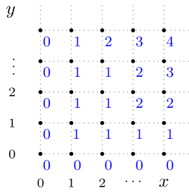
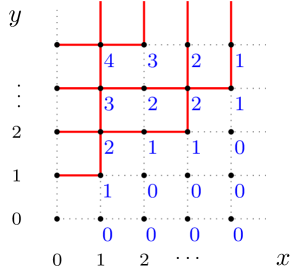
Figure 17. Left: the scalar marginal $\ell(\lambda^{(x,y)})$ of the sHL/sHL Yang-Baxter field. Right: the corresponding realization of the stochastic six vertex model with the step boundary conditions. The height function $\mathfrak{h}^{\mathrm{6V}}$ is indicated, too.

Remark 7.9.

While Theorem 7.8 essentially follows from [BP17], let us emphasize what is different here. Theorem 7.8 connects the ordinary stochastic six vertex model with stable spin Hall-Littlewood polynomials. On the other hand, previously the same stochastic six vertex model was matched to Hall-Littlewood processes and measures [BBW16], [BM18], and the non-stable spin Hall-Littlewood polynomials gave rise to a dynamic version of the stochastic six vertex model [BP17]. Therefore, formally Theorem 7.8 is a new statement.

It might seem surprising that the stochastic six vertex model $\mathfrak{h}^{\mathrm{6V}}$ is independent of $s$, while the field $\lambda^{(x,y)}$ depends on $s$. A posteriori this might be explained by the fact that the $s$-dependent stable spin Hall-Littlewood functions are eigenfunctions of the same first $q=0$ Macdonald difference operator as their $s=0$ versions, the classical Hall-Littlewood polynomials. About difference operators see Section 8 below.

Let us now turn to the marginal of the sHL/sHL field with the two-sided scaled geometric boundary conditions described in Section 7.2.2. First, consider the behavior of $\ell(\lambda^{(x,y)})$ at the boundary:

Proposition 7.10.

Consider the transition probabilities $\mathsf{U}^{[0]}$ given in (6.17). Then we have

$$\mathsf{U}^{[0]}_{\mathrm{sg}(\alpha),\mathrm{sHL}(v)}(0,i_{0}^{\prime};j_{0}^{\prime},j_{0})=\mathbf{1}_{i_{0}^{\prime}+j_{0}^{\prime}=j_{0}}\frac{(v\alpha)^{j_{0}^{\prime}}}{1+v\alpha},$$ (7.3)

$$\mathsf{U}^{[0]}_{\mathrm{sHL}(u),\mathrm{sg}(\beta)}(i_{0},0;j_{0}^{\prime},j_{0})=\mathbf{1}_{i_{0}+j_{0}=j_{0}^{\prime}}\frac{(u\beta)^{j_{0}}}{1+u\beta},$$ (7.4)

$$\mathsf{U}^{[0]}_{\mathrm{sg}(\alpha),\mathrm{sg}(\beta)}(0,0;j_{0}^{\prime},j_{0})=\mathbf{1}_{j_{0}^{\prime}=j_{0}}\frac{(\alpha\beta)^{j_{0}}}{(q;q)_{j_{0}}}(\alpha\beta;q)_{\infty}.$$ (7.5)

The cases (7.3), (7.4) correspond to the bottom and the left boundaries, respectively, and (7.5) arises in the bottom left corner. Observe that (7.5) defines the $q$-Poisson distribution (cf. Section 1.5).

Proof of Proposition 7.10.

This follows by combining (6.17) with the formulas for the boundary weights (3.1), (A.16) and the cross vertex weights (Figure 26 and (A.20)). To specialize the factor corresponding to $R^{(I,J)}_{u,v}(J,0;J,0)$ one should use Remark 7.5. ∎

Now take the stochastic six vertex model with independent Bernoulli boundary conditions (we call these the two-sided stationary or $(\alpha,\beta)$-stationary boundary conditions):

$$b^{\mathrm{h}}_{x}\sim\mathrm{Ber}\left(\frac{v_{x}\alpha}{1+v_{x}\alpha}\right)\qquad\text{and}\qquad b^{\mathrm{v}}_{y}\sim\mathrm{Ber}\left(\frac{1}{1+u_{y}\beta}\right).$$ (7.6)

That is, given a realization of these random variables, we then consider the stochastic six vertex model with these boundary conditions according to Definition 7.7. While the random path configuration in this model is well-defined, it cannot be encoded by the height function $\mathfrak{h}^{\mathrm{6V}}$ in the same way as for the step boundary conditions. Indeed, if $\alpha>0$, the number of paths to the right of any vertex $(x,y)$ is almost surely infinite. Let us thus introduce the centered height function

$$\mathcal{H}^{\mathrm{6V}}(x,y)=\#\{\textnormal{occupied horizontal edges}\}-\#\{\textnormal{occupied vertical edges}\},$$ (7.7)

where we count the edges along a directed up-right sequence of cells in the lattice, for example, moving $(\frac{1}{2},\frac{1}{2})\to(x+\frac{1}{2},\frac{1}{2})\to(x+\frac{1}{2},y+\frac{1}{2})$ along straight lines. In other words, $\mathcal{H}^{\mathrm{6V}}$ has the same gradient as $\mathfrak{h}^{\mathrm{6V}}$, but the constant is defined by $\mathcal{H}^{\mathrm{6V}}(0,0)=0$. The next lemma is a straightforward observation:

Lemma 7.11.

The centered height function $\mathcal{H}^{\mathrm{6V}}(x,y)$ well-defined and almost sure finite for all $(x,y)\in\mathbb{Z}_{\geq 0}\times\mathbb{Z}_{\geq 0}$. For $\alpha=\beta=0$ the boundary conditions (7.6) reduce to the step boundary conditions (7.2), and in this case we have $\mathcal{H}^{\mathrm{6V}}(x,y)=\mathfrak{h}^{\mathrm{6V}}(x+1,y)$ for all $x,y$.

The centered height function with the two-sided Bernoulli boundary conditions (7.6) can be identified with a marginal of the sHL/sHL Yang-Baxter field $\boldsymbol{\lambda}$ with scaled geometric boundary conditions.

Theorem 7.12.

Let $\mathcal{M}$ be the $q$-Poisson random variable with parameter $\alpha\beta$ independent of the stochastic six vertex model with $(\alpha,\beta)$-stationary boundary conditions. The two random fields $\{y-\ell(\lambda^{(x,y)}):x,y\in\mathbb{Z}_{\geq 0}\}$ and $\{\mathcal{H}^{\mathrm{6V}}(x,y)-\mathcal{M}:x,y\in\mathbb{Z}_{\geq 0}\}$ are equal in distribution.

Theorem 7.12 follows in essentially the same way as Theorem 7.8 by matching the value of vertex weights $\mathsf{L}_{u_{y},v_{x}}$ and probability laws of entries $b^{\mathrm{h}}_{x},b^{\mathrm{v}}_{x}$ with those given $\mathsf{U}^{[0]}$ (on the boundary this follows from Proposition 7.10; in fact, the structure of the concrete formulas (7.3), (7.4) is essential for the independent boundary conditions). Let us present a slightly different argument that uses analytic continuation. This alternative approach is useful in other situations (Sections 7.3 and 7.4) and also in Section 9 for computation of observables of models with two-sided stationary boundary conditions.

Proof of Theorem 7.12.

Consider the sHL/sHL Yang-Baxter field with the usual step boundary conditions, and with shifted indices:

$$\boldsymbol{\mu}=\{\mu^{(x,y)}:(x,y)\in\mathbb{Z}_{\geq-I_{0}+1}\times\mathbb{Z}_{\geq-J_{0}+1}\}.$$

Here $I_{0},J_{0}$ are positive integers. For $\boldsymbol{\mu}$ we take the following specializations:

$$u_{0},qu_{0},\dots q^{J_{0}-1}u_{0},u_{1},u_{2},\dots\qquad\text{and}\qquad v_{0},qv_{0},\dots q^{I_{0}-1}v_{0},v_{1},v_{2},\dots.$$ (7.8)

Call $\boldsymbol{\nu}=\boldsymbol{\mu}|_{{}_{\mathbb{Z}_{\geq 0}\times\mathbb{Z}_{\geq 0}}}$ the restriction of $\boldsymbol{\mu}$ to the nonnegative quadrant. Then $\boldsymbol{\nu}$ is a field of random Young diagrams associated to the sHL/sHL skew Cauchy structure with Gibbs boundary conditions (Definition 2.5). That is, for all $x,y$, the boundary Young diagrams $\nu^{(0,y)},\dots,\nu^{(0,0)},\dots,\nu^{(x,0)}$ are distributed with law

$$\frac{1}{Z_{\mathrm{boundary}}^{(x,y)}}\prod_{j=1}^{y}\mathsf{F}_{\nu^{(0,j)}/\nu^{(0,j-1)}}(u_{j})\mathfrak{G}^{(I_{0})}_{\nu^{(0,y)}}(v_{0})\prod_{i=1}^{x}\mathsf{F}^{*}_{\nu^{(i,0)}/\nu^{(i-1,0)}}(v_{i})\mathfrak{F}^{(J_{0})}_{\nu^{(x,0)}}(u_{0}),$$ (7.9)

recalling the notation introduced in Section 4. The vertex weights in the definition of the principal specialization of the sHL functions $\mathfrak{G}_{\nu^{(0,y)}}$ and $\mathfrak{F}_{\nu^{(x,0)}}$ depend on the parameters $u_{0},q^{J_{0}},v_{0},q^{I_{0}}$ in a rational way. Therefore, for any bounded complex-valued cylindric function $f:\boldsymbol{\nu}\mapsto f(\boldsymbol{\nu})$, the expected value $\mathbb{E}_{\boldsymbol{\nu}}(f)$ is a holomorphic function of $u_{0},q^{J_{0}},v_{0},q^{I_{0}}$ when these parameters are in a small neighborhood of zero.

Let $\boldsymbol{\lambda}$ be the sHL/sHL field with $(\alpha,\beta)$-scaled geometric boundary conditions. The above argument shows that the probability of any event depending on a finite region in the field $\boldsymbol{\lambda}$ is equal to the scaled geometric degeneration

$$u_{0}=-\epsilon\alpha,\quad q^{J_{0}}=1/\epsilon,\qquad v_{0}=-\epsilon\beta,\quad q^{I_{0}}=1/\epsilon,\qquad\epsilon\to 0,$$

of the probability of the same event in which the field $\boldsymbol{\lambda}$ is replaced by $\boldsymbol{\nu}$.

Consider now the stochastic six vertex model with the step boundary conditions on the shifted lattice $\mathbb{Z}_{\geq-I_{0}+1}\times\mathbb{Z}_{\geq-J_{0}+1}$, which corresponds to the field $\boldsymbol{\mu}$ (with parameters (7.8)). Refer to its height function by $\mathfrak{h}^{\mathrm{6V}(I_{0},J_{0})}$. By Theorem 7.8, we have equality in distribution

$$\mathfrak{h}^{\mathrm{6V}(I_{0},J_{0})}(x,y)\stackrel{{\scriptstyle d}}{{=}}y+J_{0}-\ell(\nu^{(x,y)})\qquad\text{for all }x,y\geq 0$$ (7.10)

(here $y+J_{0}$ is simply the shifted vertical coordinate, and $\nu^{(x,y)}=\mu^{(x,y)}$ for $x,y\geq 0$). Next, let $\mathcal{H}^{\mathrm{6V}(I_{0},J_{0})}(x,y)$ be the centered height function of the restriction of the above vertex model to the nonnegative quadrant $\mathbb{Z}_{\geq 0}^{2}$. Then

$$\mathcal{H}^{6\mathrm{V}(I_{0},J_{0})}(x,y)=\mathfrak{h}^{\mathrm{6V}(I_{0},J_{0})}(x,y)-J_{0}+\mathcal{M}_{I_{0},J_{0}}\qquad\text{for all }x,y\geq 0,$$ (7.11)

where $\mathcal{M}_{I_{0},J_{0}}$ is the random variable counting the number of paths originating from the segment $\{-I_{0}+1\}\times[-J_{0}+1,0]$ and vertically crossing the segment $[-I_{0}+1,0]\times\{0\}$. Combining (7.10) and (7.11), we find that

$$y-\ell(\nu^{(x,y)})\stackrel{{\scriptstyle d}}{{=}}\mathcal{H}^{6\mathrm{V}(I_{0},J_{0})}(x,y)-\mathcal{M}_{I_{0},J_{0}}\qquad\text{for all }x,y\geq 0.$$ (7.12)

The probability law of $\mathcal{M}_{I_{0},J_{0}}$ is found from the sHL/sHL field $\boldsymbol{\mu}$ which has step boundary conditions (hence we can use Theorem 7.8). On the other hand, the update in the initial $(I_{0},J_{0})$ part of $\boldsymbol{\mu}$ is restated as a single forward transition in the $(I_{0},J_{0})$-fused field (considered in Section 6 above). Therefore, the law of $\mathcal{M}_{I_{0},J_{0}}$ is given by (6.17) with parameters $u_{0},q^{J_{0}},v_{0},q^{I_{0}}$:

$$\mathrm{Prob}\{\mathcal{M}_{I_{0},J_{0}}=k\}=\mathsf{U}^{[0]}_{u_{0},v_{0}}(0,0;k,k)\qquad\text{for }k=0\dots,I_{0}.$$ (7.13)

Under the scaled geometric specializations to both $\alpha$ and $\beta$, this distribution becomes $q\textnormal{-}\mathrm{Poi}(\alpha\beta)$, cf. (7.5). Taking the scaled geometric specializations in (7.12), we obtain the desired matching between the centered height function $\mathcal{H}^{6\mathrm{V}}$ of the stochastic six vertex model with the $(\alpha,\beta)$-stationary boundary conditions and the marginal of the field $\boldsymbol{\lambda}$. ∎

7.3. The sHL/sqW Yang-Baxter field

Here we consider the Yang-Baxter field associated with the dual Cauchy identity between the sHL and the sqW functions. The marginal of the field is the stochastic higher spin six vertex model. We consider both step and two-sided stationary boundary conditions in the vertex model. The model with the step boundary conditions was extensively studied starting from [CP16], [BP18]. Different formulas for observables in the two-sided stationary case leading to asymptotic results were obtained recently in [IMS19] by a different method.

7.3.1. Step boundary conditions

The sHL/sqW field corresponds to setting $v=s$ and $q^{I}=-\theta/s$ in the notation of Section 6. The parameters are $q\in(0,1)$, $s\in(-1,0)$, $u\in[0,1)$, $\theta\in[-s,-s^{-1}]$. The Yang-Baxter equation governing the vertex weights is (A.12). The reversibility condition of the forward and backward transition operators is proven in the same way as Proposition 7.3, and is given as follows:

Proposition 7.13.

For any four Young diagrams $\mu,\varkappa,\lambda,\nu$ we have

$$\frac{1+u\theta}{1-us}\,\mathsf{U}^{\mathrm{fwd}}_{\mathrm{sHL}(u),\mathrm{sqW}(\theta)}(\varkappa\to\nu\mid\lambda,\mu)\,\,\mathsf{F}_{\lambda/\varkappa}(u)\mathbb{F}^{*}_{\mu^{\prime}/\varkappa^{\prime}}(\theta)\\ =\mathsf{U}^{\mathrm{bwd}}_{\mathrm{sHL}(u),\mathrm{sqW}(\theta)}(\nu\to\varkappa\mid\lambda,\mu)\,\,\mathbb{F}^{*}_{\nu^{\prime}/\lambda^{\prime}}(\theta)\mathsf{F}_{\nu/\mu}(u)$$ (7.14)

Summing (7.14) over both $\varkappa$ and $\nu$, we obtain the skew Cauchy identity of Theorem 3.9.

The sHL/sqW Yang-Baxter field $\boldsymbol{\lambda}=\{\lambda^{(x,y)}\}$ depends on the parameters $u_{y}\in[0,1)$, $\theta_{x}\in[-s,-s^{-1}]$, $x,y\in\mathbb{Z}_{\geq 1}$, and is generated from the step boundary conditions $\lambda^{(x,0)}=\lambda^{(0,y)}=0^{\infty}=\varnothing$ by applying the forward transition operators $\mathsf{U}^{\mathrm{fwd}}_{\mathrm{sHL}(u_{y}),\mathrm{sqW}(\theta_{x})}$.

Proposition 7.14.

The single-point point distributions in the sHL/sqW field with the step boundary conditions have the form

$$\mathrm{Prob}(\lambda^{(x,y)}=\nu)=\prod_{\begin{subarray}{c}1\leq i\leq x\\ 1\leq j\leq y\end{subarray}}\frac{1-u_{j}s}{1+u_{j}\theta_{i}}\,\mathsf{F}_{\nu}(u_{1},\dots,u_{y})\,\mathbb{F}^{*}_{\nu^{\prime}}(\theta_{1},\dots,\theta_{x}).$$

The joint distributions along down-right paths are expressed through the skew functions as in Proposition 2.9.

7.3.2. Scaled geometric boundary conditions

Take additional parameters $\alpha,\beta\in[0,-s^{-1}]$, and consider specializations

$$\rho^{\mathrm{v}}_{-1}=\mathrm{sg}(\alpha),\qquad\rho^{\mathrm{h}}_{-1}=\mathrm{sg}(\beta),\qquad\rho^{\mathrm{v}}_{y}=\mathrm{sHL}(u_{y}),\qquad\rho^{\mathrm{h}}_{x}=\mathrm{sqW}(\theta_{x}).$$

Let $\boldsymbol{\eta}$ be the Yang-Baxter field on the lattice $\mathbb{Z}_{\geq-1}\times\mathbb{Z}_{\geq-1}$ generated by the forward transition probabilities constructed using the specializations (dragging the cross vertex through the leftmost column should be understood as in Remark 7.5). Restricting this field to the nonnegative quadrant, $\boldsymbol{\lambda}=\boldsymbol{\eta}|_{{}_{\mathbb{Z}_{\geq 0}\times\mathbb{Z}_{\geq 0}}}$, we get the sHL/sqW field with the two-sided scaled geometric (or $(\alpha,\beta)$-scaled geometric) boundary conditions.

Proposition 7.15.

For the field $\boldsymbol{\lambda}$ defined above we have

$$\mathrm{Prob}\{\lambda^{(x,y)}=\nu\}=\frac{(\alpha\beta;q)_{\infty}}{\prod\limits_{j=1}^{y}(1+u_{j}\beta)}\prod_{i=1}^{x}\frac{(\alpha\theta_{i};q)_{\infty}}{(-s\alpha;q)_{\infty}}\prod_{\begin{subarray}{c}1\leq i\leq x\\ 1\leq j\leq y\end{subarray}}\frac{1-u_{j}s}{1+u_{j}\theta_{i}}\,\mathsf{F}_{\nu}(u_{1},\dots,u_{y};\widetilde{\alpha})\,\mathbb{F}^{*}_{\nu^{\prime}}(\theta_{1},\dots,\theta_{x};\widetilde{\beta}).$$

Joint distributions in $\boldsymbol{\lambda}$ along down-right paths are expressed similarly to Proposition 2.9.

7.3.3. Stochastic higher spin six vertex model

The Markovian marginal of the sHL/sqW field can be mapped to a known stochastic vertex model which we now recall. Let the vertex weights $\mathcal{L}_{u_{y},\theta_{x}}(i_{1},j_{1};i_{2},j_{2})$, $i_{1},i_{2}\in\mathbb{Z}_{\geq 0}$, $j_{1},j_{2}\in\left\{0,1\right\}$, be given in Figure 18. They are stochastic for our values of parameters in the sense that $\sum_{i_{2},j_{2}}\mathcal{L}_{u_{y},\theta_{x}}(i_{1},j_{1};i_{2},j_{2})=1$ for all $i_{1},j_{1}$.

Figure 18. Stochastic vertex weights $\mathcal{L}_{u,\theta}(i_{1},j_{1};i_{2},j_{2})$. This parametrization of the weights differs from the ones employed in [CP16] or [BP18], but all these parametrizations are related to each other via simple changes of variables.

Definition 7.16 ([CP16], [BP18]).

The (inhomogeneous) stochastic higher spin six vertex model with the boundary conditions $B^{\mathrm{h}}=\{b^{\mathrm{h}}_{1},b^{\mathrm{h}}_{2},\dots\}$ and $B^{\mathrm{v}}=\{b^{\mathrm{v}}_{1},b^{\mathrm{v}}_{2},\dots\}$, $b_{i}^{\mathrm{v}}\in\left\{0,1\right\}$, $b_{j}^{\mathrm{h}}\in\mathbb{Z}_{\geq 0}$, is the (unique) probability measure on the set of up-right directed paths on $\mathbb{Z}_{\geq 0}\times\mathbb{Z}_{\geq 0}$ (with multiple vertical paths allowed per edge, but at most one horizontal path per edge) satisfying:

• Each vertex $(0,y)$ at the vertical boundary $\{(0,y^{\prime}):y^{\prime}\geq 1\}$ emanates a path initially pointing to the right if $b^{\mathrm{v}}_{y}=1$;

• Each vertex $(x,0)$ at the horizontal boundary $\{(x^{\prime},0):x^{\prime}\geq 1\}$ emanates $b^{\mathrm{h}}_{x}$ paths initially pointing upward;

• For each $(x,y)$, conditioned to the path configuration at all vertices $(x^{\prime},y^{\prime})$ such that $x^{\prime}+y^{\prime}<x+y$, the probability of a vertex configuration $(i_{1},j_{1};i_{2},j_{2})$ at $(x,y)$ is given by $\mathcal{L}_{u_{y},\theta_{x}}(i_{1},j_{1};i_{2},j_{2})$. Moreover, the random choices made at diagonally adjacent vertices $\ldots,(x-1,y+1),(x,y),(x+1,y-1),\ldots$ are independent under the same condition.

In particular, the step boundary conditions correspond to paths entering horizontally at each location and no paths entering through the bottom boundary (7.2), exactly as in the stochastic six vertex case considered in Section 7.2.

Similarly to the six vertex case, let us encode the configuration of paths by the centered height function $\mathcal{H}^{\mathrm{HS}}(x,y)$, see (7.7). That is, $\mathcal{H}^{\mathrm{HS}}(0,0)=0$, and the stochastic higher spin six vertex model paths serve as level lines for $\mathcal{H}^{\mathrm{HS}}$. For the step boundary conditions we have $\mathcal{H}^{\mathrm{HS}}(x,y)=\mathfrak{h}^{\mathrm{HS}}(x+1,y)$, where $\mathfrak{h}^{\mathrm{HS}}(x,y)$ is the number of paths passing weakly to the right of the point $(x,y)\in\mathbb{Z}_{\geq 0}^{2}$.

The next proposition suggests the appropriate choice of the two-sided stationary boundary conditions for the stochastic higher spin six vertex model:

Proposition 7.17.

Consider the transition probabilities $\mathsf{U}^{[0]}$ given in (6.17). Then

$$\mathsf{U}^{[0]}_{\mathrm{sg}(\alpha),\mathrm{sqW}(\theta)}(0,i_{0}^{\prime};j_{0}^{\prime},j_{0})=\mathbf{1}_{i_{0}^{\prime}+j_{0}^{\prime}=j_{0}}(\alpha\theta)^{j_{0}^{\prime}}\,\frac{(-s/\theta;q)_{j_{0}^{\prime}}}{(q;q)_{j_{0}^{\prime}}}\frac{(\alpha\theta;q)_{\infty}}{(-s\alpha;q)_{\infty}}.$$ (7.15)

Proof.

This follows by specializing (6.17) and using the expressions for the boundary weights $W^{*},\widetilde{w}$ ((3.14) and (A.16), respectively), and the cross weights $R^{\mathrm{sqW,sg}}_{\alpha,\theta}$ (A.19). The quantity $R^{(I,J)}_{uv}(J,0;J,0)$ should be specialized as described in Remark 7.5. ∎

Let us define the stochastic higher spin six vertex model with two-sided stationary (or $(\alpha,\beta)$-stationary) boundary conditions by taking independent random variables on the boundary distributed as (recall the notation in Section 1.5)

$$b_{x}^{\mathrm{h}}\sim q\textnormal{-}\mathrm{NB}(-s/\theta_{x},\alpha\theta_{x})\qquad\text{and}\qquad b_{y}^{\mathrm{v}}\sim\mathrm{Ber}\left(\frac{1}{1+u_{x}\beta}\right).$$ (7.16)

Let $\mathcal{H}^{\mathrm{HS}}(x,y)$ be the corresponding centered height function.

For $\alpha=\beta=0$ the boundary conditions (7.16) reduce to the step one. When $\beta$ depends on $\alpha$ in a certain way, the stationarity of the boundary conditions (7.16) under the homogeneous stochastic higher spin six vertex model was checked in a continuous-time degeneration in [BP18a, Appendix B.2], see also [IMS19] for the full statement and further discussion.

The next result is the analogue of both Theorems 7.8 and 7.12 from the stochastic six vertex case. Let $\boldsymbol{\lambda}$ be the sHL/sqW Yang-Baxter field with the $(\alpha,\beta)$-scaled geometric boundary conditions.

Theorem 7.18.

Let $\mathcal{M}$ be the $q$-Poisson random variable with parameter $\alpha\beta$ independent of the stochastic higher spin six vertex model with $(\alpha,\beta)$-stationary boundary conditions. Then the two random fields $\left\{y-\ell(\lambda^{(x,y)})\colon x,y\in\mathbb{Z}_{\geq 0}\right\}$ and $\{\mathcal{H}^{\mathrm{HS}}(x,y)-\mathcal{M}\colon x,y\in\mathbb{Z}_{\geq 0}\}$ are equal in distribution.

Proof.

To obtain the matching in the step case (note that when $\alpha$ or $\beta$ is zero, $\mathcal{M}=0$ almost surely), it suffices to check that

$$\mathsf{U}^{[0]}_{\mathrm{sHL}(u),\mathrm{sqW}(\theta)}(i_{0},1-i_{0}^{\prime};j_{0}^{\prime},1-j_{0})=\mathcal{L}_{u,\theta}(i_{0},i_{0}^{\prime};j_{0}^{\prime},j_{0})$$

for all $i_{0},j_{0}^{\prime}\in\mathbb{Z}_{\geq 0}$ and $i_{0}^{\prime},j_{0}\in\left\{0,1\right\}$, where the left-hand side is the specialization of (6.17). This is a straightforward verification.

The matching result for the scaled geometric boundary conditions is obtained in the same way as in the proof of Theorem 7.12. Indeed, we can consider the field in $\mathbb{Z}_{\geq-I_{0}+1}\times\mathbb{Z}_{\geq-J_{0}+1}$ with the extra sHL specializations with the parameters $u_{0},qu_{0},\ldots,q^{J_{0}-1}u_{0}$ and $v_{0},qv_{0},\ldots,q^{I_{0}-1}v_{0}$. The desired matching then follows from the expressions (7.4), (7.5), (7.15) for the corresponding specializations of $\mathsf{U}^{[0]}$, and analytic continuation. ∎

7.4. The sqW/sqW Yang-Baxter field

Let us now turn to the third and final Yang-Baxter field associated with the sqW/sqW skew Cauchy structure. The particle system we obtain as its marginal generalizes the $q$-Hahn PushTASEP introduced recently in [CMP18].

7.4.1. Step boundary conditions

The sqW/sqW Yang-Baxter field depends on the parameters $q\in(0,1)$, $s\in[-\sqrt{q},0)$, $\theta_{x},\xi_{y}\in[-s,-s^{-1}]$. The reversibility condition associated with the forward and backward transition probabilities takes the following form:

Proposition 7.19.

For any four Young diagrams $\mu,\varkappa,\lambda,\nu$ we have

$$\frac{(-s\xi;q)_{\infty}(-s\theta;q)_{\infty}}{(s^{2};q)_{\infty}(\xi\theta;q)_{\infty}}\,\mathsf{U}^{\mathrm{fwd}}_{\mathrm{sqW}(\xi),\mathrm{sqW}(\theta)}(\varkappa\to\nu\mid\lambda,\mu)\,\mathbb{F}_{\lambda^{\prime}/\varkappa^{\prime}}(\xi)\,\mathbb{F}^{*}_{\mu^{\prime}/\varkappa^{\prime}}(\theta)\\ =\mathsf{U}^{\mathrm{bwd}}_{\mathrm{sqW}(\xi),\mathrm{sqW}(\theta)}(\nu\to\varkappa\mid\lambda,\mu)\,\mathbb{F}^{*}_{\nu^{\prime}/\lambda^{\prime}}(\theta)\,\mathbb{F}_{\nu^{\prime}/\mu^{\prime}}(\xi).$$ (7.17)

Summing (7.17) over both $\varkappa$ and $\nu$, we obtain the skew Cauchy identity of Theorem 3.12.

The sqW/sqW Yang-Baxter field with the step boundary conditions $\boldsymbol{\lambda}$ is, by definition, generated from the boundary conditions $\lambda^{(x,0)}=\lambda^{(0,y)}=0^{\infty}=\varnothing$ by applying the forward transition operators $\mathsf{U}^{\mathrm{fwd}}_{\mathrm{sqW}(\xi_{y}),\mathrm{sqW}(\theta_{x})}$.

Proposition 7.20.

The single-point distributions in the sqW/sqW field $\boldsymbol{\lambda}$ with the step boundary conditions have the form

$$\mathrm{Prob}\bigl{(}\lambda^{(x,y)}=\nu\bigr{)}=\prod_{\begin{subarray}{c}1\leq i\leq x\\ 1\leq j\leq y\end{subarray}}\frac{(s^{2};q)_{\infty}(\xi_{i}\theta_{j};q)_{\infty}}{(-s\xi_{i};q)_{\infty}(-s\theta_{j};q)_{\infty}}\,\mathbb{F}_{\nu^{\prime}}(\xi_{1},\dots,\xi_{y})\,\mathbb{F}^{*}_{\nu^{\prime}}(\theta_{1},\dots,\theta_{x}).$$

The joint distributions in $\boldsymbol{\lambda}$ along down-right paths are expressed through the skew sqW functions as in Proposition 2.9.

7.4.2. Scaled geometric boundary conditions

Let $\alpha,\beta\in[0,-s^{-1}]$ be additional parameters. The sqW/sqW Yang-Baxter field with two-sided scaled geometric (or $(\alpha,\beta)$-scaled geometric) boundary conditions is constructed exactly as in Sections 7.2.2 and 7.3.2 by adding scaled geometric specializations to both boundaries of the quadrant $\mathbb{Z}_{\geq 0}^{2}$.

Proposition 7.21.

The single-point distributions in the sqW/sqW Yang-Baxter field $\boldsymbol{\lambda}$ with $(\alpha,\beta)$-scaled geometric boundary conditions are given by

$$\mathrm{Prob}\bigl{(}\lambda^{(x,y)}=\nu\bigr{)}=(\alpha\beta;q)_{\infty}\prod_{i=1}^{x}\frac{(\alpha\theta_{i};q)_{\infty}}{(-s\alpha;q)_{\infty}}\prod_{j=1}^{y}\frac{(\beta\xi_{j};q)_{\infty}}{(-s\beta;q)_{\infty}}\\ \times\prod_{\begin{subarray}{c}1\leq i\leq x\\ 1\leq j\leq y\end{subarray}}\frac{(s^{2};q)_{\infty}(\xi_{i}\theta_{j};q)_{\infty}}{(-s\xi_{i};q)_{\infty}(-s\theta_{j};q)_{\infty}}\,\mathbb{F}_{\nu^{\prime}}(\xi_{1},\dots,\xi_{y};\widetilde{\alpha})\,\mathbb{F}^{*}_{\nu^{\prime}}(\theta_{1},\dots,\theta_{x};\widetilde{\beta}).$$

The joint distributions along down-right paths are expressed as in Proposition 2.9.

7.4.3. Stochastic vertex model with ${}_{4}\phi_{3}$ weights

The scalar marginal $\{\ell(\lambda^{(x,y)})\}$ of the sqW/sqW Yang-Baxter field gives rise to a new vertex model which is related to the $q$-Hahn PushTASEP from [CMP18] (we discuss this connection in Section 7.4.4 below). To formulate the vertex model, let us first write down the quantities (6.17) under the two sqW specializations:

$$\begin{split}&\mathbb{L}_{\xi,\theta}(i_{1},j_{1};i_{2},j_{2}):=\mathsf{U}_{\mathrm{sqW}(\xi),\mathrm{sqW}(\theta)}^{[0]}(i_{1},j_{1};i_{2},j_{2})\\ &\hskip 40.0pt=\mathbf{1}_{i_{1}+j_{2}=i_{2}+j_{1}}\,\frac{\xi^{i_{2}}s^{i_{1}}\theta^{i_{2}-i_{1}}\,q^{j_{1}j_{2}+\frac{1}{2}i_{1}(i_{1}-1)}\,(-s/\theta;q)_{i_{2}}(-s/\xi;q)_{j_{2}}}{(-s/\theta;q)_{i_{1}}(-s/\xi;q)_{j_{1}}(q;q)_{j_{2}}(-q/(s\xi);q)_{j_{2}-i_{2}}}\\ &\hskip 80.0pt\times\frac{(s^{2}q^{i_{1}+j_{2}};q)_{\infty}(\theta\xi;q)_{\infty}}{(-s\xi;q)_{\infty}(-s\theta;q)_{\infty}}\,{}_{4}\overline{\phi}_{3}\left(\begin{minipage}{147.95424pt} \centering{$q^{-j_{1}};q^{-j_{2}},-s\theta,-q/(s\xi)$} \\ \centering{$-s/\xi,q^{1+i_{1}-j_{1}},-\theta q^{1-j_{2}-i_{1}}/s$} \@add@centering\@add@centering\end{minipage}\Big{|}\,q,q\right),\end{split}$$ (7.18)

where $i_{1},j_{1},i_{2},j_{2}\in\mathbb{Z}_{\geq 0}$.

Lemma 7.22.

Let $q\in(0,1)$, $s\in[-\sqrt{q},0)$, $\xi,\theta\in[-s,-s^{-1}]$. Then $\mathbb{L}_{\xi,\theta}(i_{1},j_{1};i_{2},j_{2})\geq 0$ for all $i_{1},j_{1},i_{2},j_{2}\in\mathbb{Z}_{\geq 0}$. Moreover, $\sum_{i_{2},j_{2}}\mathbb{L}_{\xi,\theta}(i_{1},j_{1};i_{2},j_{2})=1$ for all $i_{1},j_{1}\in\mathbb{Z}_{\geq 0}$.

Proof.

The nonnegativity follows from Section A.5 (in particular, from Proposition A.8). The fact that the weights sum to one is the consequence of the Yang-Baxter equation (A.13) in the leftmost column, where $i_{3}=j_{3}=\infty$, together with Proposition A.5. ∎

The weights $\mathbb{L}_{\xi,\theta}(i_{1},j_{1};i_{2},j_{2})$ give rise to a stochastic vertex model. Because the arrow preservation property for these weights reads $i_{1}+j_{2}=i_{2}+j_{1}$, the paths in this stochastic vertex model are directed up-left.

Definition 7.23.

Let $\xi_{y},\theta_{x}\in[-s,-s^{-1}]$, $x,y\in\mathbb{Z}_{\geq 1}$. The (inhomogeneous) ${}_{4}\phi_{3}$ stochastic vertex model with the boundary conditions $\{b_{1}^{\mathrm{h}},b_{2}^{\mathrm{h}},\ldots\}$ and $\{b_{1}^{\mathrm{v}},b_{2}^{\mathrm{v}},\ldots\}$, $b_{i}^{\mathrm{h}},b_{j}^{\mathrm{v}}\in\mathbb{Z}_{\geq 0}$, is the (unique) probability distribution on the set of up-left directed paths on $\mathbb{Z}_{\geq 0}\times\mathbb{Z}_{\geq 0}$ (with arbitrary nonnegative number of paths allowed per edge, see Figure 19 for an illustration), satisfying:

• The number of paths entering at each location $(x,0)$ on the horizontal boundary is equal to $b_{x}^{\mathrm{h}}$, $x\in\mathbb{Z}_{\geq 1}$;

• The number of paths exiting at each location $(0,y)$ on the vertical boundary is equal to $b_{y}^{\mathrm{v}}$, $y\in\mathbb{Z}_{\geq 1}$;

• For each $(x,y)$, conditioned on the path configuration at all vertices $(x^{\prime},y^{\prime})$ such that $x^{\prime}+y^{\prime}<x+y$, the probability of the configuration $(i_{1},j_{1};i_{2},j_{2})$ at $(x,y)$ is given by $\mathbb{L}_{\xi_{y},\theta_{x}}(i_{1},j_{1};i_{2},j_{2})$. Moreover, the random choices made at diagonally adjacent vertices $\ldots,(x-1,y+1),(x,y),(x+1,y-1),\ldots$ are independent under the same condition.

In particular, the step boundary conditions correspond to taking $b_{i}^{\mathrm{h}}=b_{i}^{\mathrm{v}}=0$ for all $i\in\mathbb{Z}_{\geq 1}$.

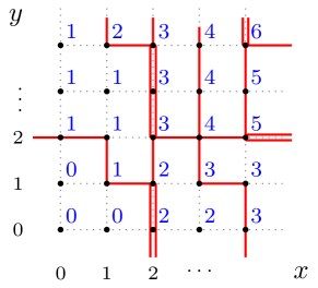
Figure 19. A path configuration in the ${}_{4}\phi_{3}$ stochastic vertex model, and the corresponding height function. (The boundary configuration in the figure are not step. Unlike for the two previous vertex models, here the step boundary conditions would mean no paths crossing the boundary.)

Remark 7.24.

The up-left direction of paths in the ${}_{4}\phi_{3}$ vertex model of Definition 7.23 should be contrasted with up-right paths in the stochastic vertex model (Section 7.2.3) and the stochastic higher spin six vertex model (Section 7.3.3). Note however that in the latter two models the number $j$ of paths per horizontal edge is at most one, and so the operation $j\mapsto 1-j$ applied at each horizontal edge turns up-right paths into up-left ones. In the sqW/sqW setting the number of paths per horizontal edge can be arbitrary, so the model with the weights $\mathbb{L}_{\xi,\theta}$ cannot be mapped to a model with up-right directed paths.

For arbitrary boundary conditions, the configuration of the paths is encoded by the height function $\mathbb{H}^{\phi}(x,y)$, $x,y\in\mathbb{Z}_{\geq 0}$, which counts the number of paths which between $(0,0)$ and $(x,y)$ (including the paths that pass through $(x,y)$, too). In other words, paths are the level lines of $\mathbb{H}^{\phi}$. An example is given in Figure 19. Clearly, $\mathbb{H}^{\phi}(x,y)$ is almost surely finite at each $(x,y)$.

Proposition 7.17 expressing $\mathsf{U}^{[0]}_{\mathrm{sg}(\alpha),\mathrm{sqW}(\theta)}$ on the bottom boundary of $\mathbb{Z}_{\geq 0}^{2}$ as the $q$-negative binomial distribution $q\textnormal{-}\mathrm{NB}(-s/\theta,\alpha\theta)$ suggests the two-sided stationary boundary conditions for the ${}_{4}\phi_{3}$ stochastic vertex model. Moreover, on the left boundary, by the symmetry (A.9), $\mathsf{U}^{[0]}_{\mathrm{sqW}(\xi),\mathrm{sg}(\beta)}$ leads to $q\textnormal{-}\mathrm{NB}(-s/\xi,\beta\xi)$. Therefore, we define the two-sided (or $(\alpha,\beta)$) stationary boundary conditions by taking independent

$$b_{x}^{\mathrm{h}}\sim q\textnormal{-}\mathrm{NB}(-s/\theta_{x},\alpha\theta_{x}),\qquad b_{y}^{\mathrm{v}}\sim q\textnormal{-}\mathrm{NB}(-s/\xi_{y},\beta\xi_{y}).$$

The step boundary condition arises when $\alpha=\beta=0$, and thus $b_{x}^{\mathrm{h}}=b_{y}^{\mathrm{v}}=0$ for all $x,y$ (note that this meaning of “step” here differs from the two previous stochastic vertex models).

Recall the $q$-Poisson distribution (Section 1.5). Let $\boldsymbol{\lambda}$ be the sqW/sqW Yang-Baxter field with $(\alpha,\beta)$-scaled geometric boundary conditions.

Theorem 7.25.

Let $\mathcal{M}$ be the $q$-Poisson random variable with parameter $\alpha\beta$ which is independent of the ${}_{4}\phi_{3}$ stochastic vertex model. Then the two random fields $\{\ell(\lambda^{(x,y)})\colon x,y\in\mathbb{Z}_{\geq 0}\}$ and $\{\mathbb{H}^{\phi}(x,y)+\mathcal{M}\colon x,y\in\mathbb{Z}_{\geq 0}\}$ have the same distribution.

Proof.

This is proven similarly to Theorems 7.12 and 7.18 using analytic continuation. Namely, one starts with the Yang-Baxter field $\boldsymbol{\mu}$ in $\mathbb{Z}_{\geq-I_{0}+1}\times\mathbb{Z}_{\geq-J_{0}+1}$, where the positive coordinates $\mathbb{Z}_{\geq 1}\times\mathbb{Z}_{\geq 1}$ carry the sqW specializations $\{\xi_{y}\}$ and $\{\theta_{x}\}$, and the extra nonpositive coordinates carry the sHL specializations with parameters $u_{0},qu_{0},\ldots,q^{J_{0}-1}u_{0}$ and $v_{0},qv_{0},\ldots,q^{I_{0}-1}v_{0}$, respectively. The resulting field depends on $u_{0},q^{J_{0}},v_{0},q^{I_{0}}$ in an analytic manner, and one can then take $u_{0},q^{J_{0}},v_{0},q^{I_{0}}$ to the scaled geometric specializations.

Before the analytic continuation we know that $\ell(\mu^{(x,y)})$ is equal in distribution to the height function $\mathbb{H}^{\phi}_{I_{0},J_{0}}(x,y)$, which is defined in the same way as $\mathbb{H}^{\phi}$, but in $\mathbb{Z}_{\geq-I_{0}+1}\times\mathbb{Z}_{\geq-J_{0}+1}$. The number of paths originating from the segment $\{-I_{0}+1\}\times[-J_{0}+1,0]$ and vertically crossing the segment $[-I_{0}+1,0]\times\{0\}$ becomes, after the scaled geometric specializations, the desired $q$-Poisson random variable $\mathcal{M}$. Therefore, after the specializations $\mathbb{H}^{\phi}_{I_{0},J_{0}}(x,y)$ turns into $\mathbb{H}^{\phi}(x,y)+\mathcal{M}$ for all $x,y\in\mathbb{Z}_{\geq 0}$. On the other hand, $\ell(\mu^{(x,y)})$ becomes $\ell(\lambda^{(x,y)})$ for all $x,y\in\mathbb{Z}_{\geq 0}$. This completes the proof. ∎

7.4.4. Connection to PushTASEPs

Take arbitrary stochastic vertex weights $\mathfrak{L}_{(x,y)}(i_{1},j_{1};i_{2},j_{2})$, $x,y\in\mathbb{Z}_{\geq 1}$, $i_{1},j_{1},i_{2},j_{2}\in\mathbb{Z}_{\geq 0}$, which vanish unless $i_{1}+j_{2}=i_{2}+j_{1}$, and construct from them a stochastic vertex model with up-left paths as in Definition 7.23. We also assume that boundary conditions $b_{x}^{\mathrm{h}}$ and $b_{y}^{\mathrm{v}}$, $x,y\in\mathbb{Z}_{\geq 1}$, are fixed. Path configurations in this vertex model can be equivalently viewed as trajectories in a stochastic particle system on the line with a pushing mechanism.

Indeed, consider the discrete time dynamics $\mathbf{y}(t)$ on the space of configurations

$$\{\mathbf{y}=(y_{1}>y_{2}>\ldots)\colon y_{i}\in\mathbb{Z}\}$$

defined as follows (see Figure 20 for an illustration):

1. At time $t=0$ we have $y_{1}(0)=-1$ and $y_{k}(0)-y_{k+1}(0)-1=b^{\mathrm{h}}_{k}$, $k\in\mathbb{Z}_{\geq 1}$;

2. At each discrete time step $t-1\to t$, $t\in\mathbb{Z}_{\geq 1}$, the first particle’s location is updated as $y_{1}(t)=y_{1}(t-1)-b_{t}^{\mathrm{v}}$ (i.e., it jumps by $b_{t}^{\mathrm{v}}$ to the left);

3. At each discrete time step $t-1\to t$, $t\in\mathbb{Z}_{\geq 1}$, the locations of the subsequent particles are updated sequentially. For $i=2,3,\ldots$, after the $(i-1)$-st particle has moved such that $y_{i-1}(t)=y_{i-1}(t-1)-l$, and if the gap was $y_{i-1}(t-1)-y_{i}(t-1)-1=g$, then the $i$-th particle jumps by $L$ to the left with probability $\mathfrak{L}_{(i,t)}(g,l;g+L-l,L)$.

The fact that it must be $L\geq l-g$ in the update implies that the dynamics preserves the order of the particles. Namely, if the jump $l$ of the $(i-1)$-st particle is longer than the gap, then the $i$-th particle is pushed to the left. Therefore, the dynamics $\mathbf{y}(t)$ has a built-in pushing mechanism.

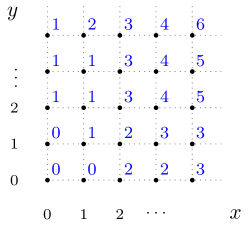
Figure 20. The height function in the vertex model (left) and the corresponding realization of the pushing dynamics (right).

At each discrete time step the dynamics $\mathbf{y}(t)$ might perform an infinite number of jumps. However, due to the sequential update structure, the evolution of the first $N$ particles $y_{1}>\ldots>y_{N}$ is always well-defined, and thus one can define the whole dynamics $\mathbf{y}(t)$ via Kolmogorov’s extension theorem.

Particle systems with pushing mechanism have been studied for a long time. The first example is the PushTASEP (also known as the “long-range TASEP”, or as a degenerate particular case of the Toom’s interface model) [Spi70], [DLSS91]. The PushTASEP admits many deformations, most recent of which is the $q$-Hahn PushTASEP introduced in [CMP18] (see also section 3.2.1 in the latter paper for references to known intermediate degenerations). Recall that the $q$-Hahn PushTASEP depends on three parameters $q\in(0,1)$, $\mu\in(0,1)$, and $\nu\in(-1,\min(\mu,\sqrt{q})]$.

Proposition 7.26.

For $\alpha=0$, $\beta=1$, $\xi_{y}=\mu$, $\theta_{x}=1$ for all $x,y\in\mathbb{Z}_{\geq 1}$, and $s=-\nu$, the particle system corresponding to the ${}_{4}\phi_{3}$ stochastic vertex model (i.e., with $\mathfrak{L}_{(i,t)}=\mathbb{L}_{\mu,1}$ given by (7.18)) and $(\alpha,\beta)$-stationary boundary conditions coincides with the $q$-Hahn PushTASEP from [CMP18] with the step initial configuration $y_{i}(0)=-i$, $i\in\mathbb{Z}_{\geq 1}$.

Proof.

This is obtained in a straightforward way by matching the formulas from [CMP18] expressing transition probabilities in the $q$-Hahn PushTASEP through the ${}_{4}\phi_{3}$ $q$-hypergeometric functions with the expression (7.18). For $\alpha=0$, there are no vertex model paths entering through the bottom boundary. Then the boundary conditions on the left are random and independent with the distribution $q\textnormal{-}\mathrm{NB}(-s/\xi,\beta\xi)=q\textnormal{-}\mathrm{NB}(\nu/\mu,\mu)$, which is exactly the jumping distribution of the $q$-Hahn PushTASEP first particle (denoted by $\varphi_{q,\mu,\nu}(\cdot\mid\infty)$ in [CMP18]). ∎

We see that the ${}_{4}\phi_{3}$ stochastic vertex model from Section 7.4.3 in a particular case becomes the $q$-Hahn PushTASEP. Note also that to match the jumping distribution of the first particle we needed to employ the independent negative binomial boundary conditions on the left (vertical) boundary. (This effect is also present in the stochastic higher spin six vertex model, cf. [OP17].) The pushing particle system corresponding to the step boundary conditions in the ${}_{4}\phi_{3}$ stochastic vertex model is more general than the $q$-Hahn PushTASEP. Namely, the former can essentially be viewed as the $q$-Hahn PushTASEP conditioned on the event that the first particle $y_{1}$ never jumps.

8. Difference operators

In this Section we prove that the (stable) spin Hall-Littlewood and the spin $q$-Whittaker functions are eigenfunctions of certain ($q$-)difference operators acting on symmetric functions. In this section we denote the quantization parameter in the sHL functions by $t$ instead of $q$ because the sHL eigenoperators are the same as in the Macdonald case (recall that for $s=0$, the sHL functions become the usual Hall-Littlewood symmetric polynomials, which are the $q=0$ degenerations of the Macdonald symmetric polynomials).

8.1. Eigenrelations for the spin Hall-Littlewood functions

Consider the space of symmetric rational functions in $u_{1},\ldots,u_{n}$. Let the operator $T_{q,u_{i}}$ on this space be

$$T_{q,u_{i}}f(u_{1},\dots,u_{n})=f(u_{1},\dots,u_{i-1},qu_{i},u_{i+1},\dots u_{n}),$$ (8.1)

that is, it acts by multiplying the variable $u_{i}$ by $q$. In this subsection we will use the $q=0$ version, $T_{0,u_{i}}$. Note that this operator acts only on rational functions whose denominators do not contain positive powers of $u_{i}$.

Definition 8.1 (Hall-Littlewood difference operators).

For $1\leq r\leq n$, let the $r$-th Hall-Littlewood difference operator be

$$\mathop{\mathfrak{D}_{r}}:=\sum_{\begin{subarray}{c}I\subset\{1,\dots,n\}\\ |I|=r\end{subarray}}\biggl{(}\prod_{\begin{subarray}{c}i\in I\\ j\in\{1,\dots,n\}\setminus I\end{subarray}}\frac{tu_{i}-u_{j}}{u_{i}-u_{j}}\biggr{)}\,T_{0,I},$$ (8.2)

with $T_{0,I}=\prod_{i\in I}T_{0,u_{i}}$.

The Hall-Littlewood operators are the $q=0$ cases of the Macdonald difference operators [Mac95, Chapter VI.3] (the latter are obtained by taking $T_{q,u_{i}}$ in (8.2) instead of $T_{0,u_{i}}$). The operators $\mathop{\mathfrak{D}_{r}}$ are diagonal in the Hall-Littlewood symmetric polynomials $\mathsf{F}_{\lambda}|_{{}_{s=0}}$:

$$\mathop{\mathfrak{D}_{r}}\mathsf{F}_{\lambda}(u_{1},\ldots,u_{n})|_{{}_{s=0}}=e_{r}(1,t,\dots,t^{n-\ell(\lambda)-1})\,\mathsf{F}_{\lambda}(u_{1},\ldots,u_{n})|_{{}_{s=0}},$$ (8.3)

where the eigenvalues are given in terms of $e_{r}(u_{1},\dots u_{n})$, the $r$-th elementary symmetric polynomial:

$$e_{r}(z_{1},\ldots,z_{N})=\sum_{1\leq i_{1}<\cdots<i_{r}\leq N}z_{i_{1}}\cdots z_{i_{r}}.$$ (8.4)

In particular, $e_{r}(z_{1},\ldots,z_{N})=0$ if $r>N$.

In the following Theorem we extend (8.3) to the spin Hall-Littlewood symmetric functions:

Theorem 8.2.

For all Young diagrams $\lambda$ and $n\in\mathbb{Z}_{\geq 1}$ we have

$$\mathop{\mathfrak{D}_{r}}\mathsf{F}_{\lambda}(u_{1},\ldots,u_{n})=e_{r}(1,t,\dots,t^{n-\ell(\lambda)-1})\,\mathsf{F}_{\lambda}(u_{1},\ldots,u_{n}).$$ (8.5)

Remark 8.3.

Certain difference operators acting diagonally on the non-stable spin Hall-Littlewood symmetric functions were considered in [Dim18].

In order to prove Theorem 8.2 we make use of two preliminary lemmas. The first one is an explicit expression for the sHL function $\mathsf{F}_{\lambda}$ as a sum over the symmetric group $\mathfrak{S}_{n}$:

Lemma 8.4.

For any Young diagram $\lambda$ such that $n\geq\ell(\lambda)$, we have

$$\mathsf{F}_{\lambda}(u_{1},\dots,u_{n})=\frac{(1-t)^{n}}{(t;t)_{n-\ell(\lambda)}}\sum_{\sigma\in\mathfrak{S}_{n}}\sigma\biggl{\{}\prod_{1\leq i<j\leq n}\frac{u_{i}-tu_{j}}{u_{i}-u_{j}}\prod_{i=1}^{n}\left(\frac{u_{i}-s}{1-su_{i}}\right)^{\lambda_{i}}\,\prod_{i=1}^{\ell(\lambda)}\frac{u_{i}}{u_{i}-s}\biggr{\}}.$$ (8.6)

Here the symmetric group acts on the indices of the variables $u_{i}$, but not on $\lambda_{i}$.

Proof.

This is a corollary of [Bor17, Theorem 5.1] which gives an analogous expression for the non-stable spin Hall-Littlewood function. The degeneration to the stable case is obtained as in (3.7). Symmetrization formula (8.6) for the stable case appeared earlier in [GGW17] and [BW17]. ∎

Lemma 8.5.

We have

$$\mathop{\mathfrak{D}_{r}}\biggl{(}\sum_{\sigma\in\mathfrak{S}_{n}}\sigma\biggl{\{}\prod_{1\leq i<j\leq n}\frac{u_{i}-tu_{j}}{u_{i}-u_{j}}\biggr{\}}\biggr{)}=e_{r}(1,\dots,t^{n-1})\sum_{\sigma\in\mathfrak{S}_{n}}\sigma\biggl{\{}\prod_{1\leq i<j\leq n}\frac{u_{i}-tu_{j}}{u_{i}-u_{j}}\biggr{\}}.$$ (8.7)

Proof.

This is the $\lambda=\varnothing$ case of the known Hall-Littlewood relation (8.3). Notice that the symmetrized sum in fact does not depend on the variables $u_{1},\ldots,u_{n}$:

$$\sum_{\sigma\in\mathfrak{S}_{n}}\sigma\biggl{\{}\prod_{1\leq i<j\leq n}\frac{u_{i}-tu_{j}}{u_{i}-u_{j}}\biggr{\}}=\frac{(t;t)_{n}}{(1-t)^{n}},$$

see [Mac95, Chapter III.1, formula (1.4)]. ∎

Proof of Theorem 8.2.

For a fixed Young diagram $\lambda$ we define

$$A=\prod_{1\leq i<j\leq n}\frac{u_{i}-tu_{j}}{u_{i}-u_{j}},\qquad B=\prod_{i=1}^{n}\left(\frac{u_{i}-s}{1-su_{i}}\right)^{\lambda_{i}},\qquad C=\prod_{i=1}^{\ell(\lambda)}\frac{u_{i}}{u_{i}-s}.$$

With this notation, using (8.6), the left-hand side of (8.5) can be written as

$$c_{\lambda}\sum_{\begin{subarray}{c}I\subset\{1,\dots,n\}\\ |I|=r\end{subarray}}\prod_{\begin{subarray}{c}i\in I\\ j\in\{1,\dots,n\}\setminus I\end{subarray}}\frac{tu_{i}-u_{j}}{u_{i}-u_{j}}\,T_{0,I}\sum_{\sigma\in\mathfrak{S}_{n}}\sigma\left\{ABC\right\},$$ (8.8)

where $c_{\lambda}=(1-t)^{n}/(t;t)_{n-\ell(\lambda)}$. We first observe that

$$T_{0,I}\sigma\{C\}=\begin{cases}\sigma\{C\}\qquad&\text{if }I\subseteq\{\sigma_{\ell(\lambda)+1},\dots,\sigma_{n}\},\\ 0\qquad&\text{otherwise}.\end{cases}$$

Therefore, we can reduce the sum over the symmetric group in (8.8) to permutations $\sigma$ such that $I\subseteq\sigma(\{\ell(\lambda)+1,\dots,n\})$. Moreover, we see that the claim of Theorem 8.2 follows for $r>n-\ell(\lambda)$ since both sides of (8.5) vanish. Thus we will now assume that $r\leq n-\ell(\lambda)$.

For a given permutation $\sigma$ define the ordered sets $V_{\sigma},W_{\sigma}$ as

$$V_{\sigma} =\sigma(\{1,\dots,\ell(\lambda)\})=\left\{v_{1},\ldots,v_{\ell(\lambda)}\right\},$$

$$W_{\sigma} =\sigma(\{\ell(\lambda)+1,\dots,n\})=\{w_{1},\ldots,w_{n-\ell(\lambda)}\}=I\cup K,$$

and rewrite (8.8) as

$$c_{\lambda}\sum_{\begin{subarray}{c}I\subset\{1,\dots,n\}\\ |I|=r\end{subarray}}\sum_{\begin{subarray}{c}\sigma\in\mathfrak{S}_{n}\\ I\subseteq W_{\sigma}\end{subarray}}\sigma\left\{BC\right\}\prod_{\begin{subarray}{c}i\in I\\ j\in\{1,\dots,n\}\setminus I\end{subarray}}\frac{tu_{i}-u_{j}}{u_{i}-u_{j}}\,T_{0,I}\sigma\left\{A\right\},$$ (8.9)

where we used the fact that $\sigma\{BC\}$ only depends on variables $u_{j}$ for $j\in V_{\sigma}$. We now focus on the remaining factors. For two disjoint or coinciding ordered sets $S_{1},S_{2}$ denote $P(S_{1},S_{2}):=\prod_{i\in S_{1},\,j\in S_{2}}\frac{u_{i}-tu_{j}}{u_{i}-u_{j}}$. When $S_{1}=S_{2}$, the product is only over $i<j$. We have

$$\prod_{\begin{subarray}{c}i\in I\\ j\in\{1,\dots,n\}\setminus I\end{subarray}}\frac{tu_{i}-u_{j}}{u_{i}-u_{j}}\,T_{0,I}\sigma\left\{A\right\}=P(I^{c},I)P(V_{\sigma},V_{\sigma})P(V_{\sigma},K)$$

$$\hskip 190.0pt\times T_{0,I}\Bigl{(}P(I,K)P(I,I)P(V_{\sigma},I)P(K,I)P(K,K)\Bigr{)}$$

$$\hskip 15.0pt=P(V_{\sigma},V_{\sigma})P(V_{\sigma},W_{\sigma})P(K,I)\,T_{0,I}\Bigl{(}P(I,K)P(I,I)P(K,K)\Bigr{)}$$

$$\hskip 15.0pt=\prod_{1\leq i<j\leq\ell(\lambda)}\frac{u_{v_{i}}-tu_{v_{j}}}{u_{v_{i}}-u_{v_{j}}}\prod_{i\in V_{\sigma},\,j\in W_{\sigma}}\frac{u_{i}-tu_{j}}{u_{i}-u_{j}}\prod_{i\in W_{\sigma}\setminus I,j\in I}\frac{u_{i}-tu_{j}}{u_{i}-u_{j}}\,T_{0,I}\prod_{1\leq i<j\leq n-\ell(\lambda)}\frac{u_{w_{i}}-tu_{w_{j}}}{u_{w_{i}}-u_{w_{j}}}.$$

In the above calculation we used the fact that $T_{0,I}$ acts on $P(S,I)$, $S\neq I$, by turning it into one. The action $T_{0,I}P(I,I)$ does not make sense before the symmetrization (i.e., summation over $\sigma$), and so we do not apply $T_{0,I}$ to this expression just yet. In the last line, the first two products are independent of $I$ and of the ordering of $W_{\sigma}$, and the last two products are independent of the ordering of $V_{\sigma}$. Therefore, we can rearrange the two summations in (8.9) as

$$\begin{split}&c_{\lambda}\sum_{\begin{subarray}{c}V\subseteq\{1,\dots,n\}\\ |V|=\ell(\lambda),\,W=V^{c}\end{subarray}}\sum_{\tau\in\mathfrak{S}_{\ell(\lambda)}}\prod_{\begin{subarray}{c}v\in V\\ w\in W\end{subarray}}\frac{u_{v}-tu_{w}}{u_{v}-u_{w}}\,\tau\biggl{\{}\prod_{1\leq i<j\leq\ell(\lambda)}\frac{u_{v_{i}}-tu_{v_{j}}}{u_{v_{i}}-u_{v_{j}}}\,BC\biggr{\}}\\ &\hskip 80.0pt\times\sum_{\begin{subarray}{c}I\subset W\\ |I|=r\end{subarray}}\,\prod_{\begin{subarray}{c}i\in I\\ w\in W\setminus I\end{subarray}}\frac{tu_{i}-u_{w}}{u_{i}-u_{w}}\,T_{0,I}\sum_{\sigma\in\mathfrak{S}_{n-\ell(\lambda)}}\sigma\biggl{\{}\prod_{1\leq i<j\leq n-\ell(\lambda)}\frac{u_{w_{i}}-tu_{w_{j}}}{u_{w_{i}}-u_{w_{j}}}\biggr{\}}.\end{split}$$ (8.10)

The permutations $\tau,\sigma$ permute the variables $u_{v_{i}},u_{w_{j}}$, $v_{i}\in V$, $w_{j}\in W$, acting respectively on indices $i$ and $j$. We can now employ Lemma 8.5 to transform the second line of (8.10) into

$$e_{r}(1,t,\dots,t^{n-\ell(\lambda)-1})\sum_{\sigma\in\mathfrak{S}_{n-\ell(\lambda)}}\sigma\biggr{\{}\prod_{1\leq i<j\leq n-\ell(\lambda)}\frac{u_{w_{i}}-tu_{w_{j}}}{u_{w_{i}}-u_{w_{j}}}\biggr{\}}.$$ (8.11)

Therefore,

$$\begin{split}\text{lhs \eqref{eq:sHL_eigen} }&=e_{r}(1,t,\dots,t^{n-\ell(\lambda)-1})\,c_{\lambda}\sum_{\begin{subarray}{c}V\subseteq\{1,\dots,n\}\\ |V|=\ell(\lambda),\,W=V^{c}\end{subarray}}\;\sum_{\begin{subarray}{c}\tau\in\mathfrak{S}_{\ell(\lambda)}\\ \sigma\in\mathfrak{S}_{n-\ell(\lambda)}\end{subarray}}\prod_{\begin{subarray}{c}v\in V\\ w\in W\end{subarray}}\frac{u_{v}-tu_{w}}{u_{v}-u_{w}}\\ &\qquad\times\sigma\biggl{\{}\prod_{1\leq i<j\leq n-\ell(\lambda)}\frac{u_{w_{i}}-tu_{w_{j}}}{u_{w_{i}}-u_{w_{j}}}\biggr{\}}\;\tau\biggl{\{}\prod_{1\leq i<j\leq\ell(\lambda)}\frac{u_{v_{i}}-tu_{v_{j}}}{u_{v_{i}}-u_{v_{j}}}\,BC\biggr{\}}.\end{split}$$ (8.12)

The summations in the right-hand side of this last expression (along with the factor $c_{\lambda}$) are easily rearranged into the symmetrized sum (8.6) producing the spin Hall Littlewood function $\mathsf{F}_{\lambda}$. ∎

8.2. Orthogonality

The spin Hall-Littlewood functions enjoy the following orthogonality:

Proposition 8.6.

For any Young diagrams $\lambda,\mu$, we have

$$\frac{(t;t)_{n-\ell(\lambda)}}{(1-t)^{n}n!}\oint_{\gamma}\frac{dz_{1}}{2\pi\mathrm{i}z_{1}}\cdots\oint_{\gamma}\frac{dz_{n}}{2\pi\mathrm{i}z_{n}}\prod_{1\leq i\neq j\leq n}\frac{z_{i}-z_{j}}{z_{i}-tz_{j}}\,\mathsf{F}_{\lambda}(z_{1},\dots,z_{n})\mathsf{F}^{*}_{\mu}(1/z_{1},\dots,1/z_{n})=\mathbf{1}_{\lambda=\mu},$$ (8.13)

where $\gamma$ is a positively oriented contour encircling $0$, $t^{k}s$ for all $k\geq 0$, and the contour $t\gamma$ (its image under the multiplication by $t$), but not the point $s^{-1}$.

Proof.

This is consequence of [BP18, Corollary 7.5], where an analogous result is stated for the non-stable spin Hall-Littlewood functions with inhomogeneous parameters (the corresponding homogeneous result goes back to [BCPS15]). The desired orthogonality relation (8.13) then follows with the help of the limit (3.7). ∎

The orthogonality property (8.13) resembles the orthogonality of the Hall-Littlewood polynomials with respect to the Macdonald’s torus scalar product [Mac95, Chapter VI, (9.10)] at $q=0$. The general $(q,t)$ scalar product is

$$\langle f,g\rangle_{n}:=\frac{1}{(2\pi\mathrm{i})^{n}n!}\int_{\mathbb{T}^{n}}f(z)\overline{g(z)}\prod_{1\leq i\neq j\leq n}\frac{(z_{i}/z_{j};q)_{\infty}}{(tz_{i}/z_{j};q)_{\infty}}\prod_{i=1}^{n}\frac{dz_{i}}{z_{i}},$$ (8.14)

where the integration is over the $n$-dimensional torus in $\mathbb{C}^{n}$ (i.e., over the positively oriented unit circles). In the presence of the additional spin parameter $s$, the Hall-Littlewood orthogonality extends to (8.13).

The usual $q$-Whittaker polynomials are orthogonal with respect to (8.14) with $t=0$. At present it is not clear how to extend this orthogonality property to the spin $q$-Whittaker polynomials. This problem could be related to the following observation. While all the $q=0$ Macdonald difference operators are diagonal in the spin Hall-Littlewood functions (as well as in the usual Hall-Littlewood polynomials), the situation on the spin $q$-Whittaker side is more complicated. In the next subsection we discuss an $s$-deformation of the first $t=0$ Macdonald $q$-difference operator which acts diagonally on the spin $q$-Whittaker polynomials.

8.3. Eigenrelation for the spin $q$-Whittaker polynomials

Fix $l\in\mathbb{Z}_{\geq 1}$. Define the operator acting on rational functions in $(\theta_{1},\ldots,\theta_{l})$:

$$\mathop{\mathfrak{E}}:=\sum_{j=1}^{l}\left(1+\frac{s}{\theta_{j}}\right)^{l}\biggl{(}\prod_{i\neq j}\frac{\theta_{j}}{\theta_{j}-\theta_{i}}\biggr{)}T_{q^{-1},\theta_{j}}+\frac{(-s)^{l}}{\theta_{1}\cdots\theta_{l}}\,Id.$$ (8.15)

Here $T_{q^{-1},\theta_{j}}$ are the shifts (8.1), and $Id$ is the identity operator.

Theorem 8.7.

For any Young diagram $\lambda$, we have

$$\mathfrak{E}\,\mathbb{F}_{\lambda}(\theta_{1},\ldots,\theta_{l})=q^{-\lambda_{1}}\mathbb{F}_{\lambda}(\theta_{1},\ldots,\theta_{l}).$$ (8.16)

Remark 8.8.

When $s=0$, the operator $\mathfrak{E}$ reduces to the first Macdonald operator with $t=0$ and the parameter $q^{-1}$ instead of $q$. Then (8.16) turns into the known eigenrelation for the usual $q$-Whittaker polynomials (cf. the operators $\tilde{D}_{n}^{r}$ with $r=1$ in [BC14, Section 2.2.3]). It is not clear whether there exist appropriate $s$-deformations of the higher $t=0$ Macdonald difference operators which would be diagonal in the spin $q$-Whittaker polynomials.

Theorem 8.7 follows from a “duality” relation for $\mathfrak{E}$ in Lemma 8.9 below. Define

$$\widetilde{\mathop{\mathfrak{D}}}:=q^{-n}\left(Id+(q-1)\mathop{\mathfrak{D}_{1}}\right),$$ (8.17)

where $\mathop{\mathfrak{D}_{1}}$ is the first Hall-Littlewood operator (8.2) with parameter $t$ replaced by $q$.

Lemma 8.9.

Consider the function

$$\Pi(u_{1},\dots,u_{n};\theta_{1},\dots,\theta_{l})=\prod_{i=1}^{n}\prod_{j=1}^{l}\frac{1+u_{i}\theta_{j}}{1-su_{i}}.$$ (8.18)

Then we have

$$\mathfrak{E}\,\Pi=\widetilde{\mathfrak{D}}\Pi,$$ (8.19)

where the operator $\widetilde{\mathop{\mathfrak{D}}}$ acts in $u_{1},\dots,u_{n}$, while $\mathop{\mathfrak{E}}$ acts in $\theta_{1},\dots,\theta_{l}$.

Proof.

When $\mathop{\mathfrak{E}}$ acts on a factorized function $G(\theta_{1},\dots,\theta_{l})=g(\theta_{1})\cdots g(\theta_{l})$, it admits the integral representation

$$\mathfrak{E}\,G(\theta_{1},\dots,\theta_{l})=G(\theta_{1},\dots,\theta_{l})\frac{1}{2\pi\mathrm{i}}\oint_{\gamma_{0,\boldsymbol{\theta}}}\,\prod_{i=1}^{l}\frac{z+s}{z-\theta_{i}}\frac{g(q^{-1}z)}{g(z)}\frac{dz}{z}.$$ (8.20)

Here $\gamma_{0,\boldsymbol{\theta}}$ is a positively oriented contour (or a union of contours) encircling $0$, $\theta_{i}$ for $i=1,\dots,l$, and no other singularity of the integrand. Here the function $g(z)$ should be such that we can choose a contour in whose neighborhood the expression $g(q^{-1}z)/g(z)$ is holomorphic, and such that no singularities of $g(q^{-1}z)/g(z)$ fall inside $\gamma_{0,\boldsymbol{\theta}}$.

Analogously, the action of $\widetilde{\mathop{\mathfrak{D}}}$ on $H(u_{1},\dots,u_{n})=h(u_{1})\cdots h(u_{n})$, where $h(0)=1$, has the form

$$\widetilde{\mathfrak{D}}H(u_{1},\dots,u_{n})=H(u_{1},\dots,u_{n})\frac{1}{2\pi\mathrm{i}}\oint_{\gamma_{0,\boldsymbol{u}}}\prod_{j=1}^{n}\frac{w-q^{-1}u_{j}}{w-u_{j}}\frac{1}{h(w)}\frac{dw}{w}.$$ (8.21)

The contour $\gamma_{0,\boldsymbol{u}}$ is positively oriented and contains $0$, $u_{i}$ for $i=1,\dots,n$ and no other singularity of the integrand (again, under suitable assumptions on $h(w)$). Both integral expressions (8.20) and (8.21) follow by straightforward residue calculus.

Let now both operators $\mathfrak{E}$ and $\widetilde{\mathfrak{D}}$ act on the function $\Pi$ (8.18) which has product form in both families of variables $u_{i}$ and $\theta_{j}$. We assume that $1+\theta_{j}u_{i}\neq 0$ for all $i,j$ (otherwise $\Pi$ is identically zero). From (8.20) we have

$$\frac{{\mathfrak{E}}\,\Pi(u_{1},\dots,u_{n};\theta_{1},\dots,\theta_{l})}{\Pi(u_{1},\dots,u_{n};\theta_{1},\dots,\theta_{l})}=\frac{1}{2\pi\mathrm{i}}\oint_{\gamma_{0,\boldsymbol{\theta}}}\prod_{i=1}^{l}\frac{z+s}{z-\theta_{i}}\prod_{j=1}^{n}\frac{1+q^{-1}u_{j}z}{1+u_{j}z}\frac{dz}{z}.$$

On the other hand, from (8.21) we have

$$\frac{\widetilde{{\mathfrak{D}}}\,\Pi(u_{1},\dots,u_{n};\theta_{1},\dots,\theta_{l})}{\Pi(u_{1},\dots,u_{n};\theta_{1},\dots,\theta_{l})}=\frac{1}{2\pi\mathrm{i}}\oint_{\gamma_{0,\boldsymbol{u}}}\prod_{j=1}^{n}\frac{w-q^{-1}u_{j}}{w-u_{j}}\prod_{i=1}^{l}\frac{1-sw}{1+\theta_{i}w}\frac{dw}{w}.$$

The previous two expressions are identical after a change of variables $w=-1/z$ (note that the extra minus sign corresponds to changing the contour’s orientation). ∎

Proof of Theorem 8.7.

First recall the Cauchy identity between the sHL and sqW functions (Section 3.7):

$$\sum_{\lambda}\mathsf{F}_{\lambda}(u_{1},\dots,u_{n})\mathbb{F}^{*}_{\lambda^{\prime}}(\theta_{1},\dots,\theta_{l})=\Pi(u_{1},\dots,u_{n};\theta_{1},\dots,\theta_{l}),$$ (8.22)

Combining (8.19) with (8.22) and employing the eigenrelation of sHL functions given by Theorem 8.2, we obtain

$$\sum_{\mu}\mathsf{F}_{\mu}(u_{1},\dots,u_{n})\,{\mathfrak{E}}\,\mathbb{F}^{*}_{\mu^{\prime}}(\theta_{1},\dots,\theta_{l})=\sum_{\mu}q^{-\ell(\mu)}\mathsf{F}_{\mu}(u_{1},\dots,u_{n})\mathbb{F}^{*}_{\mu^{\prime}}(\theta_{1},\dots,\theta_{l}).$$ (8.23)

This implies the equality between single terms of the summations due to orthogonality of the sHL functions (Proposition 8.6). Because $\ell(\mu)=\mu_{1}^{\prime}$, we get the desired eigenrelation. ∎

9. Fredholm determinants for marginal processes

Here we derive Fredholm determinant expressions for the $q$-Laplace transform of the random variable $-\ell(\lambda^{(x,y)})$, where $\boldsymbol{\lambda}=\{\lambda^{(x,y)}\}$ is one of the Yang-Baxter fields described in Section 7. In the sHL/sHL case, these Fredholm formulas are known [BCG16], [Agg18]. In the sHL/sqW case, they are present in the literature for the step and step-stationary boundary conditions [CP16], [BP18], [BP18a]. A Fredholm determinantal formula for the stochastic higher spin six vertex model appears also in the recent work [IMS19], though here we establish a different formula for this case. In the sqW/sqW case, a similar Fredholm formula for the $q$-Hahn PushTASEP was recently conjectured in [CMP18], and here we prove this conjecture.

In this section we return to calling the main quantization parameter by $q$ throughout.

9.1. Six vertex model observables through difference operators

In this subsection we rederive known results about the $q$-moments of the six vertex model [BCG16], [BP18] making use of the difference operators acting on spin Hall-Littlewood functions. Consider the inhomogeneous stochastic six vertex model with the step boundary conditions and height function $\mathfrak{h}^{\mathrm{6V}}$. Recall that the model depends on the parameters $v_{x}$ and $u_{y}$, $x,y\in\mathbb{Z}_{\geq 1}$, which we assume positive (cf. Section 7.2.3). Let $u_{1},u_{2},\dots$ be spaced in such a way that

$$q\sup_{i}\{u_{i}\}<\inf_{i}\{u_{i}\}.$$ (9.1)

Proposition 9.1.

Under (9.1) we have

$$\begin{split}\mathbb{E}^{\mathrm{step}}\bigl{(}q^{l\,\mathfrak{h}^{\mathrm{6V}}(x+1,y)}\bigr{)}&=q^{l(l-1)/2}\oint_{\gamma[\mathbf{u}|1]}\cdots\oint_{\gamma[\mathbf{u}|l]}\prod_{1\leq A<B\leq l}\frac{z_{A}-z_{B}}{z_{A}-qz_{B}}\\ &\hskip 30.0pt\times\prod_{k=1}^{l}\left\{\prod_{i=1}^{y}\frac{qz_{k}-u_{i}}{z_{k}-u_{i}}\prod_{i=1}^{x}\frac{1-z_{k}v_{i}}{1-qz_{k}v_{i}}\frac{dz_{k}}{2\pi\mathrm{i}z_{k}}\right\},\end{split}$$ (9.2)

where the positively orientated contour $\gamma[\mathbf{u}|j]=\gamma_{\mathbf{u}}\cup r^{j-1}C_{0}$ for $z_{j}$ is the union of a curve $\gamma_{\mathbf{u}}$ that encircles $u_{1},\dots,u_{y}$ and no other pole of the integrand, and the dilation $r^{j-1}C_{0}$ of an arbitrary small circle $C_{0}$ around $0$. Moreover, $r>q^{-1}$, and the shifted contour $q\gamma_{\mathbf{u}}$ must lie completely to the left of $\gamma_{\mathbf{u}}$ and completely to the right of $r^{l-1}C_{0}$.

Proof.

This is an application of the eigenrelations from Theorem 8.2. Recall the operator $\widetilde{\mathop{\mathfrak{D}}}$ (8.17) acting diagonally on the sHL functions as

$$\widetilde{\mathop{\mathfrak{D}}}\mathsf{F}_{\lambda}=q^{-\ell(\lambda)}\mathsf{F}_{\lambda}.$$

From Section 7.2 we have the identification $\mathfrak{h}^{\mathrm{6V}}(x+1,y)=y-\ell(\lambda^{(x,y)})$, where $\lambda^{(x,y)}$ is the sHL/sHL field. Therefore, we have

$$\mathbb{E}^{\mathrm{step}}\bigl{(}q^{l\,\mathfrak{h}^{\mathrm{6V}}(x+1,y)}\bigr{)}=q^{ly}\,\frac{\widetilde{\mathfrak{D}}^{l}\Pi(u_{1},\dots,u_{y};v_{1},\dots,v_{x})}{\Pi(u_{1},\dots,u_{y};v_{1},\dots,v_{x})},$$

where

$$\Pi(u_{1},\dots,u_{y};v_{1},\dots,v_{x})=\prod_{i=1}^{y}\prod_{j=1}^{x}\frac{1-qu_{i}v_{j}}{1-u_{i}v_{j}}.$$

The nested contour formula (9.2) follows by recursively applying integral expression (8.21) for the action of $\widetilde{\mathfrak{D}}$ on factorized functions. ∎

Proposition 9.1 combined with well-known manipulations of summations of nested contour integrals like (9.2) (e.g., see [BCS14, Section 3]) give rise to a Fredholm determinant expression for the one-point distribution of $\mathfrak{h}^{\mathrm{6V}}$.

Theorem 9.2.

Consider the stochastic six vertex model with step boundary conditions. We have

$$\mathbb{E}^{\mathrm{step}}\left(\frac{1}{(\zeta q^{\mathfrak{h}^{\mathrm{6V}}(x+1,y)};q)_{\infty}}\right)=\det\left(Id+\mathsf{K}\right)_{L^{2}(\mathsf{C})},\qquad\zeta\in\mathbb{C}\setminus{\mathbb{R}_{>0}}.$$ (9.3)

The expression in the right-hand side of (9.3) is the Fredholm determinant of the kernel

$$\mathsf{K}(w,w^{\prime})=\frac{1}{2\mathrm{i}}\int_{d+\mathrm{i}\mathbb{R}}\frac{(-\zeta)^{r}}{\sin(\pi r)}\frac{\mathsf{f}(w)/\mathsf{f}(q^{r}w)}{q^{r}w-w^{\prime}}\,dr,$$ (9.4)

where $d\in(0,1)$, and

$$\mathsf{f}(w)=\prod_{i=1}^{y}(w-u_{i})^{-1}\prod_{i=1}^{x}(1-v_{i}w).$$

The kernel $\mathsf{K}$ is defined on the Hilbert space $L^{2}(\mathsf{C})$, where $\mathsf{C}$ is a closed positively oriented curve encircling $0,u_{1},u_{2},\dots$ such that, for all $r\in d+\mathrm{i}\mathbb{R}$, $\mathsf{C}$ contains $q^{r}\mathsf{C}$ but not $q^{-r}v_{i}^{-1}$ for $i=1,2,\dots$.

We present the main steps of the proof of the Fredholm determinantal formula, and refer to [BC14] or [BCS14] for detailed explanations.

Idea of proof of Theorem 9.2.

Assume first (9.1) and $|\zeta|<1/q$, and consider the nested contour expression (9.2). We can deform all contours, one by one, to be the same $\mathsf{C}$ around $0,u_{1},u_{2},\dots$, and such that $\mathsf{C}$ contains its image under multiplication by $q$. This contour shift will cross poles $z_{A}=qz_{B}$, $A<B$, and one can rewrite (9.2) as

$$(q;q)_{l}\sum_{\lambda\vdash l}\frac{1}{m_{1}!m_{2}!\cdots}\int_{\mathsf{C}}\cdots\int_{\mathsf{C}}\,\det_{i,j=1}^{\ell(\lambda)}\left(\frac{1}{w_{i}-q^{\lambda_{j}}w_{j}}\right)\prod_{k=1}^{\ell(\lambda)}f(w_{k})/f(q^{\lambda_{k}}w_{k})\frac{dz_{k}}{2\pi\mathrm{i}},$$

where the sum is taken over all partitions $\lambda$ of $l$, and $m_{i}=m_{i}(\lambda)$ are the multiplicities of the parts $i$ in $\lambda$. Summing over $l$, we have

$$\sum_{l\geq 0}\frac{\zeta^{l}}{(q;q)_{l}}\,\mathbb{E}^{\mathrm{step}}\bigl{(}q^{l\,\mathfrak{h}^{\mathrm{6V}}(x+1,y)}\bigr{)}=\mathbb{E}^{\mathrm{step}}\left(\frac{1}{(\zeta q^{\mathfrak{h}^{\mathrm{6V}}(x+1,y)};q)_{\infty}}\right),$$

where we used the absolute summability of the left-hand side (since $0<q^{l\,\mathfrak{h}^{\mathrm{6V}}}<1$ and we assumed $|\zeta|<1/q$) to exchange the summation with the expectation sign and the $q$-binomial theorem. The result we obtain is the Fredholm determinant of the kernel

$$\sum_{n\geq 0}\frac{\zeta^{n}}{w^{\prime}-q^{n}w}\mathsf{f}(w)/\mathsf{f}(q^{n}w)=\frac{1}{2\mathrm{i}}\int_{d+\mathrm{i}\mathbb{R}}\frac{(-\zeta)^{r}}{\sin(\pi r)}\frac{\mathsf{f}(w)/\mathsf{f}(q^{r}w)}{q^{r}w-w^{\prime}}.$$

Once we reach (9.3), we can relax conditions on $u_{i}$’s and $\zeta$ since both side are analytic functions of their parameters. Formula (9.3) holds for any choice of $u_{i},v_{j}\in(0,1)$ and $\zeta\in\mathbb{C}\setminus q^{\mathbb{Z}_{\geq 0}}$ (in particular, we can always find $d$ in (9.4) such that $\mathsf{C}$ satisfies the required properties). ∎

In the next theorem we perform fusion of the sHL parameters. Recall the principal specializations $\mathfrak{F}^{(J_{0},\dots,J_{y})}(u_{0},\dots,u_{y}),\mathfrak{G}^{(I_{0},\dots,I_{x})}(v_{0},\dots,v_{x})$ defined in (4.1), (4.2). Parameters $u_{l},J_{l},v_{k},I_{k}$ are complex numbers satysfying (4.5) which we reproduce here:

$$|s|,|u_{k}|,|v_{l}|,|q^{J_{k}}u_{k}|,|q^{I_{l}}v_{l}|,\left|\frac{q^{i}u_{k}-s}{1-q^{i}su_{k}}\right|,\left|\frac{q^{i}v_{l}-s}{1-q^{i}sv_{l}}\right|<\delta\qquad\text{for all }0\leq k\leq y,\ 0\leq l\leq x,\ i\geq 0.$$ (9.5)

for sufficiently small $\delta>0$ which might depend on $x,y$, but not on the other parameters.

Theorem 9.3.

With the above notation, we have for all $\zeta\in\mathbb{C}\setminus{\mathbb{R}_{>0}}$:

$$\begin{split}&\prod_{\begin{subarray}{c}0\leq k\leq y\\ 0\leq j\leq x\end{subarray}}\frac{(u_{k}v_{l};q)_{\infty}(u_{k}v_{l}q^{I_{l}+J_{k}};q)_{\infty}}{(u_{k}v_{l}q^{I_{l}};q)_{\infty}(u_{k}v_{l}q^{J_{k}};q)_{\infty}}\\ &\hskip 70.0pt\times\sum_{\lambda}\frac{\mathfrak{F}_{\lambda}^{(J_{0},\dots,J_{y})}(u_{0},\dots,u_{y})\mathfrak{G}^{(I_{0},\dots,I_{x})}_{\lambda}(v_{0},\dots,v_{x})}{(\zeta q^{-\ell(\lambda)};q)_{\infty}}=\det\left(Id+K\right)_{L^{2}(C)}.\end{split}$$ (9.6)

The kernel $K$ is defined as

$$K(w,w^{\prime})=\frac{1}{2\mathrm{i}}\int_{d+\mathrm{i}\mathbb{R}}\frac{\bigl{(}-\zeta\bigr{)}^{r}}{\sin(\pi r)}\frac{f(w)/f(q^{r}w)}{q^{r}w-w^{\prime}}dr,$$

where $d\in(0,1)$ and

$$f(w)=\prod_{k=0}^{y}\frac{(q^{J_{k}}u_{k}/w;q)_{\infty}}{(u_{k}/w;q)_{\infty}}\prod_{l=0}^{x}\frac{(v_{l}w;q)_{\infty}}{(q^{I_{l}}v_{l}w;q)_{\infty}}.$$

The contour $C$ is a closed positively oriented curve encircling $0,q^{k}u_{i}$ for $k,i\geq 0$ and such that, for all $r\in d+\mathrm{i}\mathbb{R}$, $C$ contains $q^{r}C$ and $q^{r+k}q^{J_{l}}u_{l}$ for all $k,l\geq 0$, but leaves outside $1/(q^{r+k}v_{l})$ and $1/(q^{k}q^{I_{l}}v_{l})$ for all $k,l\geq 0$.

Proof.

Considering principal specializations in Theorem 9.2, we see that (9.6) holds for any $J_{0},\dots J_{y},I_{0},\dots,I_{x}$ positive integers. Indeed, this follows from the computation for $I,J\in\mathbb{Z}_{\geq 1}$:

$$\begin{split}&\frac{q^{r}w-u}{w-u}\frac{q^{r}w-qu}{w-qu}\ldots\frac{q^{r}w-uq^{J-1}}{w-uq^{J-1}}\frac{1-vw}{1-q^{r}vw}\frac{1-qvw}{1-q^{r}qvw}\ldots\frac{1-q^{I-1}vw}{1-q^{r}q^{I-1}vw}\\ &\hskip 40.0pt=q^{rJ}\frac{(uq^{J}/w;q)_{\infty}}{(u/w;q)_{\infty}}\frac{(q^{-r}u/w;q)_{\infty}}{(q^{-r}uq^{J}/w;q)_{\infty}}\frac{(vw;q)_{\infty}}{(vq^{I}w;q)_{\infty}}\frac{(vq^{I}wq^{r};q)_{\infty}}{(vwq^{r};q)_{\infty}}.\end{split}$$ (9.7)

The factor $q^{rJ}$ (leading to $q^{r(J_{0}+\ldots+J_{y})}$ in the kernel) disappears after replacing $\zeta$ by $\zeta q^{-J_{0}-\ldots-J_{y}}$. This change of variable accounts for the fact that in the left-hand side of (9.6) we take the $q$-Laplace transform of $q^{-\ell(\lambda)}$ as opposed to the height function in Theorem 9.2.

By the absolute convergence result of Proposition 4.4 and the boundedness of $1/(\zeta q^{-\ell(\lambda)};q)_{\infty}$, the left-hand side of (9.6) is an analytic function of $q^{J_{k}},q^{I_{l}}$ under the bounds (9.5). In order to establish the analyticity of the Fredholm determinant we first observe that, due to the compactness of $C$ and of the image of $r\to q^{r}$ for $r\in d+\mathrm{i}\mathbb{R}$, there exists a constant $M_{1}$ independent of $J_{k}$ or $I_{l}$ such that

$$\sup_{\begin{subarray}{c}w,w^{\prime}\in C,\\ r\in d+\mathrm{i}\mathbb{R}\end{subarray}}\left|\frac{f(w)/f(q^{r}w)}{q^{r}w-w^{\prime}}\right|<M_{1}.$$

This implies that $|K(w,w^{\prime})|<M_{2}$ integrating over $r$ due to the exponential decay of $1/\sin\pi r$ for large $|r|$. We can thus estimate the Fredholm determinant of $K$ with

$$\sum_{l\geq 0}\frac{1}{l!}\int_{C}\cdots\int_{C}\left|\det_{i,j=1}^{l}(K(w_{i},w_{j}))\right|dw_{1}\cdots dw_{l}\leq\sum_{l\geq 0}\frac{l^{l/2}M_{3}^{l}}{l!},$$

where we used the Hadamard inequality to bound the determinant of $K(w_{i},w_{j})$, and $M_{3}=M_{2}\ell(C)$. This shows that the right-hand side of (9.6) is an absolutely convergent sum of analytic functions and hence it is analytic. This completes the proof. ∎

Remark 9.4.

Fredholm determinantal expression (9.6) degenerates to a number of known results. In particular, considering the specialization $u_{0}=-\alpha\epsilon$, $v_{0}=-\beta\epsilon$ $q^{J_{0}}=q^{I_{0}}=1/\epsilon$, $\epsilon\to 0$, and $J_{1}=\ldots=J_{y}=I_{1}=\ldots=I_{x}=1$, we recover the expression for the $q$-Laplace transform of the height function of the six vertex model with two-sided stationary bound conditions from [Agg18, Proposition 4.1] (in the latter one has to set $\mu=0$). The latter formula is obtained by a more involved analytic continuation in $q^{J_{0}}$ than in the proof of Theorem 9.3.

9.2. Higher spin six vertex model observables

The eigenrelations for the sqW or sHL functions give rise to moment formulas for the stochastic higher spin six vertex model. Consider the model with step-Bernoulli boundary conditions $\alpha=0$, $\beta\neq 0$ (see Section 7.3). Assume that the parameters $\beta,\theta_{1},\theta_{2},\dots$ are spaced in such a way that

$$q\inf\left\{(-1/\theta_{i})_{i\geq 1}\cup(-1/\beta)\right\}>\sup\left\{(-1/\theta_{i})_{i\geq 1}\cup(-1/\beta)\right\}.$$ (9.8)

Let $\mathfrak{h}^{\mathrm{HS}}(x,y)$ be the height function of this model, i.e., the number of paths in the vertex model which are weakly to the right of the point $(x,y)$.

Following the same approach as in the proof of Proposition 9.1 (applying either $\widetilde{\mathfrak{D}}$ or $\mathfrak{E}$ from Section 8 to the sum of the corresponding Cauchy identity), we obtain a $q$-moment formula which was first written down in [CP16]:

Proposition 9.5.

We have

$$\begin{split}\mathbb{E}\left(q^{l\,\mathfrak{h}^{\mathrm{HS}}(x+1,y)}\right)&=(-1)^{l}q^{l(l-1)/2}\oint_{\Gamma[\boldsymbol{\theta},\beta|1]}\cdots\oint_{\Gamma[\boldsymbol{\theta},\beta|l]}\prod_{1\leq A<B\leq l}\frac{z_{A}-z_{B}}{z_{A}-qz_{B}}\\ &\hskip 30.0pt\times\prod_{k=1}^{l}\left\{\prod_{i=1}^{y}\frac{qz_{k}-u_{i}}{z_{k}-u_{i}}\prod_{i=1}^{x}\frac{1-z_{k}s}{1+z_{k}\theta_{i}}\frac{1}{1+\beta z_{k}}\frac{dz_{k}}{2\pi\mathrm{i}z_{k}}\right\},\end{split}$$ (9.9)

where the positively oriented contour $\Gamma[\boldsymbol{\theta},\beta|j]$ is around $-1/\beta,-1/\theta_{1},\dots-1/\theta_{x}$, $q\Gamma[\boldsymbol{\theta},\beta|j+1]$, and no other pole of the integrand.

The observable with both $\alpha,\beta$ nonzero (i.e., with the two-sided stationary boundary conditions) admits the following Fredholm determinantal expression:

Theorem 9.6.

Consider the higher spin six vertex model with two-sided stationary boundary conditions with parameters $\alpha,\beta$. Let $\mathcal{H}^{\mathrm{HS}}$ be the centered height function of this model (cf. Section 7.3), and let $\mathcal{M}\sim q\textnormal{-}\mathrm{Poi}(\alpha\beta)$ be independent of the vertex model. Then we have

$$\mathbb{E}\left(\frac{1}{(\zeta q^{\mathcal{H}^{\mathrm{HS}}(x,y)-\mathcal{M}};q)_{\infty}}\right)=\det(Id+\mathcal{K})_{L^{2}\left(\mathcal{C}\right)}.$$ (9.10)

The kernel $\mathcal{K}$ is defined by

$$\mathcal{K}(w,w^{\prime})=\frac{1}{2\mathrm{i}}\int_{d+\mathrm{i}\mathbb{R}}\frac{(-\zeta)^{r}}{\sin(\pi r)}\frac{\mathpzc{f}(w)/\mathpzc{f}(q^{r}w)}{q^{r}w-w^{\prime}}dr,$$ (9.11)

where $d\in(0,1)$ and

$$\mathpzc{f}(w)=\frac{(-\alpha/w;q)_{\infty}}{(-\beta w;q)_{\infty}}\prod_{l=1}^{y}\frac{1}{w-u_{l}}\prod_{l=1}^{x}\frac{(sw;q)_{\infty}}{(-\theta_{l}w;q)_{\infty}}.$$ (9.12)

Here $\mathcal{C}$ is a closed complex contour encircling $0,u_{1},u_{2},\dots$ and such that for all $r\in d+\mathrm{i}\mathbb{R}$, $\mathcal{C}$ contains $-q^{r+k}\alpha$ for all $k\geq 0$, but leaves outside $1/(q^{r+k}s)$ and $-1/(q^{k}\beta),1/(q^{k}\theta_{l})$ for all $k,l\geq 0$.

Proof.

We use an analytic continuation argument staring from identity (9.6). Considering specializations $\mathrm{sg}(\alpha)$ for $u_{0},q^{J_{0}}$ and $\mathrm{sg}(\beta),\mathrm{sqW}(\theta_{1}),\mathrm{sqW}(\theta_{2}),\dots$, respectively for $v_{0},q^{J_{0}},v_{1},q^{J_{1}},v_{2},q^{J_{2}},\dots$, we can prove expression (9.10) for values $\alpha,u_{l},\beta,\theta_{l}$ is a small neighborhood of the origin. Once (9.10) is established for parameters in an open set, we can perform an analytic continuation, always keeping them in a region where they define a probability measure. This is possible since both sides of (9.10) can be written as absolutely convergent series of holomorphic functions in $\alpha,u_{l},\beta,\theta_{l}$. ∎

Using the integral expression for the $q$-moments (9.9) we can obtain an alternative expression for the Fredholm determinant:

Theorem 9.7.

Assume conditions (9.8). Let $\widetilde{\mathcal{C}}$ be a closed positively oriented contour encircling $-1/\beta,-1/\theta_{1},-1/\theta_{2},\dots$ and which does not contain any point of the interior of $q\,\widetilde{\mathcal{C}}$. Then the Fredholm determinantal formula (9.10) holds when replacing $\mathcal{C}$ with $\widetilde{\mathcal{C}}$.

Proof.

The $\alpha=0$ case of this Theorem can be shown following the steps outlined in the proof of Theorem 9.2 (which in turn goes along the lines of [BC14], [BCS14]). When $\alpha>0$ a $q$-moment expansion of the $q$-Laplace transform is not possible since the $l$-th $q$-moment becomes infinite for $l$ large enough. In order to include the case where $\alpha>0$, we first produce a result analogous to that of Theorem 9.3 and subsequently we use analytic continuation.

We start by restating the result for $\alpha=0$ as

$$\prod_{k=1}^{y}\frac{1}{1+u_{k}\beta}\prod_{\begin{subarray}{c}1\leq k\leq y\\ 1\leq j\leq x\end{subarray}}\frac{1-u_{k}s}{1+u_{k}\theta_{j}}\sum_{\lambda}\frac{\mathsf{F}_{\lambda}(u_{1},\dots,u_{y})\mathbb{F}^{*}_{\lambda^{\prime}}(\theta_{1},\dots,\theta_{x};\widetilde{\beta})}{(\zeta q^{y-\ell(\lambda)};q)_{\infty}}=\det\left(Id+\mathcal{K}\,\big{|}_{\alpha=0}\right)_{L^{2}(\widetilde{\mathcal{C}})},$$ (9.13)

where we used $y-\ell(\lambda^{(x,y)})\stackrel{{\scriptstyle d}}{{=}}\mathfrak{h}^{\mathrm{HS}}(x+1,y)$, and the summation in the left hand side of (9.13) makes sense for $u_{i},\theta_{i},\beta,s$ in a complex neighborhood of the origin (under (9.8)). We can consider principal specializations of the sHL function and write the more general identity

$$\begin{split}&\prod_{k=0}^{y}\frac{(-u_{k}q^{J_{k}}\beta;q)_{\infty}}{(-u_{k}\beta;q)_{\infty}}\prod_{\begin{subarray}{c}0\leq k\leq y\\ 1\leq j\leq x\end{subarray}}\frac{(u_{k}s;q)_{\infty}(-\theta_{j}u_{k}q^{J_{k}};q)_{\infty}}{(u_{k}q^{J_{k}}s;q)_{\infty}(-\theta_{j}u_{k};q)_{\infty}}\\ &\hskip 40.0pt\times\sum_{\lambda}\frac{\mathfrak{F}^{(J_{0},\dots,J_{y})}_{\lambda}(u_{0},\dots,u_{y})\mathbb{F}^{*}_{\lambda^{\prime}}(\theta_{1},\dots,\theta_{x};\widetilde{\beta})}{(\zeta q^{J_{0}+\cdots+J_{y}-\ell(\lambda)};q)_{\infty}}=\det\bigl{(}Id+\widetilde{\mathcal{K}}\bigr{)}_{L^{2}(\widetilde{\mathcal{C}})},\end{split}$$

which again holds for $u_{i},q^{J_{i}}u_{i},\beta,\theta_{i}$ close to the origin. Here $\widetilde{\mathcal{K}}$ is given by (9.11) up to replacing $\zeta$ by $\zeta q^{J_{0}+\dots+J_{y}-y}$, and $\mathpzc{f}$ by

$$\widetilde{\mathpzc{f}}(w)=\frac{1}{(-\beta w;q)_{\infty}}\prod_{l=0}^{y}\frac{(q^{J_{l}}u_{l}/w;q)_{\infty}}{(u_{l}/w;q)_{\infty}}\prod_{l=1}^{x}\frac{(sw;q)_{\infty}}{(-\theta_{l}w;q)_{\infty}}.$$

(here we used computation (9.7)). We can now replace $\zeta$ by $\zeta q^{-J_{0}}$ in both sides of (9.2), and specialize parameters $u_{l},q^{J_{l}}u_{l}$ as $\mathrm{sg}(\alpha),\mathrm{sHL}(u_{1}),\dots\mathrm{sHL}(u_{y})$ to deduce the claim of the theorem for $\alpha,u_{l},\beta,\theta_{l},s$ in a neighborhood of the origin. Indeed, under this specialization we take $J_{1}=\ldots=J_{y}=1$, and so in the left-hand side we obtain the observable $(\zeta q^{y-\ell(\lambda)};q)_{\infty}^{-1}$, and in the right-hand side the extra power $q^{ry}$ is absorbed by going back from $\widetilde{\mathpzc{f}}(w)$ to $\mathpzc{f}(w)$ (9.12). The analytic restrictions on the parameters $\alpha,\beta,u_{l},\theta_{k},s$ can be further relaxed since both the $q$-Laplace transform and the Fredholm determinant are well defined and analytic when the parameters correspond to a probability measure and, moreover, satisfy (9.8). ∎

Remark 9.8.

Another Fredholm determinantal formula for the stochastic higher spin six vertex model with two-sided stationary boundary conditions was obtained recently in [IMS19]. While this formula differs from ours, one should in principle be able to transform one to the other. We do not focus on this in the present work.

9.3. ${}_{4}\phi_{3}$ stochastic vertex model observables.

By using the fact that the ${}_{4}\phi_{3}$ vertex model is equivalent in distribution to a marginal of the sqW/sqW field we can obtain contour integral expressions for the $q$-moments of the height function $\mathbb{H}^{\phi}$ (described in Section 7.4). Indeed, this is possible by employing the eigenoperator $\mathfrak{E}$. However, only finitely many of the $q$-moments exist, and this also involves certain bounds on the parameters. Consider the model with step-stationary boundary conditions $\alpha=0,\beta\neq 0$. Assume that $\beta,\theta_{1},\theta_{2},\dots$ satisfy (9.8).

Proposition 9.9.

If $l$ is such that $q^{l}>\max_{1\leq t\leq y}\{\beta\xi_{t}\}$, we have

$$\begin{split}\mathbb{E}^{\mathrm{step}}\left(q^{-l\,\mathbb{H}^{\phi}(x,y)}\right)&=(-1)^{l}q^{l(l-1)/2}\oint_{\Gamma[\boldsymbol{\theta},\beta|1]}\cdots\oint_{\Gamma[\boldsymbol{\theta},\beta|l]}\prod_{1\leq A<B\leq l}\frac{z_{A}-z_{B}}{z_{A}-qz_{B}}\\ &\hskip 30.0pt\times\prod_{k=1}^{l}\left\{\prod_{i=1}^{t}\frac{z_{k}-s/q}{z_{k}+\xi_{i}/q}\prod_{i=1}^{x}\frac{1-z_{k}s}{1+z_{k}\theta_{i}}\frac{1}{1+\beta z_{k}}\frac{dz_{k}}{2\pi\mathrm{i}z_{k}}\right\},\end{split}$$ (9.14)

where $\Gamma[\boldsymbol{\theta},\beta|j]$ is a positively oriented contour around $-1/\beta,-1/\theta_{1},\dots-1/\theta_{x}$, $q\Gamma[\boldsymbol{\theta},\beta|j+1]$, and no other pole of the integrand. In case $q^{l}\leq\max_{1\leq t\leq y}\{\beta\xi_{t}\}$ we have $\mathbb{E}^{\mathrm{step}}_{\phi\mathrm{VM}}\left(q^{-l\,\mathbb{H}^{\phi}(x,y)}\right)=\infty$.

Despite the fact that the distribution of $\mathbb{H}^{\phi}$ is not characterized by its $q$-moments since only finitely many of them exist, we can still write down Fredholm determinant expressions for the $q$-Laplace transform of $\mathbb{H}^{\phi}$.

Theorem 9.10.

Consider the ${}_{4}\phi_{3}$ stochastic vertex model with two-sided stationary boundary conditions with parameters $(\alpha,\beta)$. Let $\mathcal{M}\sim q\textnormal{-}\mathrm{Poi}(\alpha\beta)$ be independent of the vertex model. We have

$$\mathbb{E}_{\phi\mathrm{VM}(\alpha,\beta)}\bigl{(}\frac{1}{(\zeta q^{-\mathbb{H}^{\phi}(x,y)-\mathcal{M}};q)_{\infty}}\bigr{)}=\det(Id+\mathbb{K})_{L^{2}\left(\mathfrak{C}\right)}.$$ (9.15)

The kernel $\mathbb{K}$ is defined by

$$\mathbb{K}(w,w^{\prime})=\frac{1}{2\mathrm{i}}\int_{d+\mathrm{i}\mathbb{R}}\frac{(-\zeta)^{r}}{\sin(\pi r)}\frac{\mathbb{f}(w)/\mathbb{f}(q^{r}w)}{q^{r}w-w^{\prime}}dr,$$ (9.16)

where $d\in(0,1)$ and

$$\mathbb{f}(w)=\frac{(-\alpha/w;q)_{\infty}}{(-\beta w;q)_{\infty}}\prod_{l=1}^{y}\frac{(-\xi_{l}/w;q)_{\infty}}{(s/w;q)_{\infty}}\prod_{l=1}^{x}\frac{(sw;q)_{\infty}}{(-\theta_{l}w;q)_{\infty}}.$$ (9.17)

Here $\mathfrak{C}$ is a closed complex contour encircling $0,q^{k}s$ for $k\geq 0$ and such that, for any $r\in d+\mathrm{i}\mathbb{R}$, $\mathfrak{C}$ contains $q^{r}\mathfrak{C}$ and $-q^{r+k}\xi_{l},-q^{r+k}\alpha$ for all $k,l\geq 0$, but leaves outside $1/(q^{r+k}s)$ and $-1/(q^{k}\theta_{l}),1/(q^{k}\beta)$ for all $k,l\geq 0$.

Proof.

Expression (9.15) is derived from the general summation identity (9.6) in the same way as Theorem 9.6. First we establish (9.15) for parameters $\alpha,\beta,s,\xi_{l},\theta_{l}$ is a small neighborhood of the origin by considering specializations of $u_{0},q^{J_{0}},u_{1},q^{J_{1}},\dots,v_{0},q^{I_{0}},v_{1},q^{I_{1}}$ in (9.6). Subsequently we relax conditions on these parameters moving them away from the origin but keeping them in real intervals in such a way that they always define a probability measure. This is possible due to the analyticity of both sides of (9.15) in the parameters. ∎

Theorem 9.11.

Assume (9.8) and let $\widetilde{\mathfrak{C}}$ be a closed complex contour encircling $-1/\beta,-1/\theta_{1},-1/\theta_{2},\dots$ and that does not contain any point of the interior of $q\,\widetilde{\mathfrak{C}}$. Then expression (9.15) holds with contour $\mathfrak{C}$ replaced by $\widetilde{\mathfrak{C}}$.

Proof.

This alternative determinantal expression for the $q$-Laplace transform follows from Theorem 9.7 using the sqW specializations and subsequent analytic continuation. ∎

Remark 9.12.

Both Theorems 9.10 and 9.11 degenerate to Fredholm determinantal formulas for the $q$-Hahn pushTASEP. In particular, expression given by Theorem 9.11 was conjectured in [CMP18] (Conjecture 3.11) for step initial conditions. Therefore, we have established this conjecture. Moreover, by sending all parameters to $1$, one can also get the proof of [CMP18, Conjecture 4.6] on the Laplace transform of the one-point observable in the beta polymer like model introduced in [CMP18].

Appendix A Yang-Baxter equations

Here we review the Yang-Baxter equations used throughout the paper.

A.1. Basic cases

All Yang-Baxter equations we use can be traced to the following basic one:

Proposition A.1.

Consider the vertex weights $w,r$ defined respectively in Figure 6 and Figure 21. Then we have

$$\begin{split}&\sum_{k_{1},k_{2},k_{3}}r_{u/v}(i_{2},i_{1};k_{2},k_{1})\,w_{v,s}(i_{3},k_{1};k_{3},j_{1})\,w_{u,s}(k_{3},k_{2};j_{3},j_{2})\\ &\hskip 50.0pt=\sum_{k_{1},k_{2},k_{3}}w_{v,s}(k_{3},i_{1};j_{3},k_{1})\,w_{u,s}(i_{3},i_{2};k_{3},k_{2})\,r_{u/v}(k_{2},k_{1};j_{2},j_{1})\end{split}$$ (A.1)

for all $i_{1},i_{2},j_{1},j_{2}\in\left\{0,1\right\}$ and $i_{3},j_{3}\in\mathbb{Z}_{\geq 0}$. A visual representation of this equation is given in Figure 22.

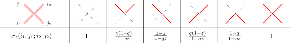
Figure 21. In the top row we see all acceptable configurations of paths entering and exiting a vertex; below we reported the corresponding vertex weights $r_{z}(i_{1},j_{1};i_{2},j_{2})$.

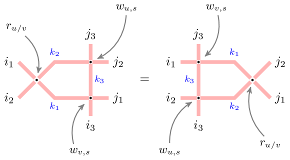
Figure 22. A schematic representation of the Yang-Baxter equation (A.1).

Proof of Proposition A.1.

This is established by a straightforward verification. Equation (A.1) appeared in several other works, including [Man14], [Bor17], [BW17]. ∎

As explained in Section 3.4, from vertex weights $w_{u,s}$ one can define the dual weights $w^{*}_{v,s}$ by changing $u$ to $1/v$, swapping the value of horizontal occupation numbers $0\leftrightarrow 1$, and multiplying by $(s-v)/(1-sv)$ in order to assign weight $1$ to the empty configuration. These manipulations clearly preserve the structure of the Yang-Baxter equation, provided that the same swapping of the occupation numbers is applied to the cross weight $r_{z}$. This leads to the definition of the cross weight $R_{z}$, see Figure 23, also normalized so that the empty configuration has weight $1$.

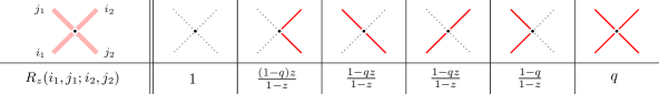
Figure 23. The cross vertex weights $R_{z}(i_{1},j_{1};i_{2},j_{2})$.

Proposition A.2.

Consider the vertex weights $w,w^{*}$ and $R$, defined respectively in Figures 6 and 8, and Figure 23. Then we have

$$\begin{split}&\sum_{k_{1},k_{2},k_{3}}R_{uv}(i_{2},i_{1};k_{2},k_{1})\,w^{*}_{v,s}(i_{3},k_{1};k_{3},j_{1})\,w_{u,s}(k_{3},k_{2};j_{3},j_{2})\\ &\hskip 50.0pt=\sum_{k_{1},k_{2},k_{3}}w^{*}_{v,s}(k_{3},i_{1};j_{3},k_{1})\,w_{u,s}(i_{3},i_{2};k_{3},k_{2})\,R_{uv}(k_{2},k_{1};j_{2},j_{1})\end{split}$$ (A.2)

for all $i_{1},i_{2},j_{1},j_{2}\in\left\{0,1\right\}$ and $i_{3},j_{3}\in\mathbb{Z}_{\geq 0}$.

A.2. Fusion

Through a fusion procedure we generalize vertex weights $w_{u,s}$ and allow configurations with multiple paths crossing a vertex in the horizontal direction. This technique of generalizing solutions to the Yang-Baxter equation was originally introduced in [KRS81] and consist in collapsing together a series of vertically attached vertices with spectral parameters forming a geometric progression of ratio $q$. The fusion of vertex weights also admits a probabilistic interpretation [CP16], [BP18], [BW17].

Define the fused vertex weight

$$\begin{split}w_{u,s}^{(J)}(i_{1},j_{1};i_{2},j_{2})&=\mathbf{1}_{i_{1}+j_{1}=i_{2}+j_{2}}\,\frac{(-1)^{i_{1}+j_{2}}q^{\frac{1}{2}i_{1}(i_{1}-1+2j_{1})}s^{j_{2}-i_{1}}u^{i_{1}}(u/s;q)_{j_{1}-i_{2}}(q;q)_{j_{1}}}{(q;q)_{i_{1}}(q;q)_{j_{2}}(su;q)_{j_{1}+i_{1}}}\\ &\qquad\qquad\times{}_{4}\overline{\phi}_{3}\left(\begin{minipage}{113.81102pt} \centering{$q^{-i_{1}};q^{-i_{2}},suq^{J},qs/u$}\\ \centering{$s^{2},q^{1+j_{2}-i_{1}},q^{1-i_{2}-j_{2}+J}$} \@add@centering\@add@centering\end{minipage}\Big{|}\,q,q\right),\end{split}$$ (A.3)

where ${}_{4}\overline{\phi}_{3}$ is the regularized $q$-hypergeometric series (1.4). Here $J$ is originally a positive integer representing the number of vertices which were fused together. However, it is easy to see that $w^{(J)}$ depends on $q^{J}$ in a rational way, thus $q^{J}$ can be regarded as the fourth independent parameter in (A.3) (along with $u,s$, and $q$). Since the regularized series ${}_{4}\overline{\phi}_{3}$ terminates, (A.3) depends on all these parameters in a rational way. Moreover, in case $i_{1},i_{2}\to\infty$, the weight $w$ loses its dependence of $j_{1}$ and we have

$$\lim_{n\to\infty}w^{(J)}_{u,s}(n,j_{1};n+j_{1}-j_{2},j_{2})=(-uq^{J})^{j_{2}}\frac{(q^{-J};q)_{j_{2}}}{(q;q)_{j_{2}}}\frac{(suq^{J};q)_{\infty}}{(su;q)_{\infty}}.$$ (A.4)

Just as in the $J=1$ case, the fused boundary weight is obtained removing the normalization factor from (A.4), and we define

$$w^{(J)}_{u,s}\biggl{(}\leavevmode\hbox to40.64pt{\vbox to33.73pt{\text{[drawing]}}}\biggr{)}\,=(-uq^{J})^{k}\frac{(q^{-J};q)_{k}}{(q;q)_{k}}. \infty \infty k \infty \infty k$$ (A.5)

This normalization is needed to assign weight 1 to the empty configuration of paths in the grid. The fused analog of the dual weights $w$ is defined similarly to (3.8):

$$w^{*,(I)}_{v,s}(i_{1},j_{1};i_{2},j_{2})=\frac{(s^{2};q)_{i_{1}}(q;q)_{i_{2}}}{(q;q)_{i_{1}}(s^{2};q)_{i_{2}}}\,w^{(I)}_{v,s}(i_{2},j_{1};i_{1};j_{2}).$$ (A.6)

These quantities also depend on $v,s,q$, and $q^{I}$ in a rational way.

What makes the fused weights remarkable is that they satisfy a general version of the Yang-Baxter equation (previously in Section A.1 the horizontal occupation numbers had to be either 0 or 1). In order to state this equation we need to consider the fusion of the cross weights $R_{z}$ leading to

$$\begin{split}R_{z}^{(I,J)}\left(i_{1},j_{1};i_{2},j_{2}\right)&:=\mathbf{1}_{i_{2}+j_{1}=i_{1}+j_{2}}\,\frac{q^{i_{2}i_{1}+\frac{1}{2}j_{2}(j_{2}-1)+j_{2}J}(-z)^{j_{2}}(q;q)_{j_{1}}}{(z;q)_{j_{1}+i_{2}}(q;q)_{j_{2}}(q;q)_{i_{2}}(q^{1-J}/z;q)_{i_{1}-j_{1}}}\\ &\qquad\qquad\times{}_{4}\overline{\phi}_{3}\left(\begin{minipage}{119.50148pt} \centering{$q^{-i_{2}};q^{-i_{1}},zq^{I},q^{1-J}/z$}\\ \centering{$q^{-J},q^{1+j_{2}-i_{2}},q^{1-i_{1}-j_{2}+I}$} \@add@centering\@add@centering\end{minipage}\Big{|}\,q,q\right).\end{split}$$ (A.7)

Proposition A.3.

Consider the weights $w^{(J)},w^{*,(I)}$ and $R^{(I,J)}$ defined in (A.3), (A.6), (A.7). Then we have

$$\begin{split}&\sum_{k_{1},k_{2},k_{3}}R_{uv}^{(I,J)}(i_{2},i_{1};k_{2},k_{1})\,w^{*,(I)}_{v,s}(i_{3},k_{1};k_{3},j_{1})\,w^{(J)}_{u,s}(k_{3},k_{2};j_{3},j_{2})\\ &\hskip 50.0pt=\sum_{k_{1},k_{2},k_{3}}w^{*,(I)}_{v,s}(k_{3},i_{1};j_{3},k_{1})\,w^{(J)}_{u,s}(i_{3},i_{2};k_{3},k_{2})\,R_{uv}^{(I,J)}(k_{2},k_{1};j_{2},j_{1}),\end{split}$$ (A.8)

for all admissible values of $i_{1},i_{2},j_{1},j_{2}$ (that is, $i_{1},j_{1}\in\left\{0,1,\ldots,I-1\right\}$ for $I$ a positive integer, or $i_{1},j_{1}\in\mathbb{Z}_{\geq 0}$ if $q^{I}$ is generic, and similarly for $i_{2},j_{2}$), and $i_{3},j_{3}\in\mathbb{Z}_{\geq 0}$. See Figure 11 for an illustration.

Note that in (A.8) (and in all other Yang-Baxter equations in this Appendix) for fixed boundary occupation numbers $i_{1},i_{2},i_{3},j_{1},j_{2},j_{3}$ the sums over $k_{1},k_{2},k_{3}$ in both sides are finite due to arrow preservation, so there are no convergence issues when $i_{3}$ and $j_{3}$ are finite. For situations with infinitely many paths one has to impose certain restrictions on parameters, cf. Definition 5.2 and Proposition 6.7.

Remark A.4.

The fused cross weights $R^{(I,J)}$ inherit symmetries of the unfused weight $R$ of Figure 23. One of these is given by the identity

$$R^{(I,J)}_{z}(i_{1},j_{1};i_{2},j_{2})=R^{(J,I)}_{z}(j_{1},i_{1};j_{2},i_{2})$$ (A.9)

for all $i_{1},j_{1},i_{2},j_{2}\in\mathbb{Z}_{\geq 0}$.

Proposition A.5.

Consider the vertex weight $R^{(I,J)}_{z}$ defined in (A.7). Then we have

$$\sum_{k_{1},k_{2}}R_{z}^{(I,J)}(a_{2},a_{1};k_{1},k_{2})=R_{z}^{(I,J)}(0,I;0,I)=R_{z}^{(I,J)}(J,0;J,0)=\frac{(zq^{I};q)_{\infty}(zq^{J};q)_{\infty}}{(z;q)_{\infty}(zq^{I+J};q)_{\infty}}$$ (A.10)

for all $a_{1},a_{2}\in\mathbb{Z}_{\geq 0}$.

Proof.

The second and the third equalities in (A.10) follow, after algebraic manipulations, from the definition of the fused cross weight $R^{(I,J)}_{z}$ given in (A.7).

The first equality in (A.10) is a trivial check in the case when $I=J=1$, using the definition of $R_{z}$ of Figure 23. It lifts to more general $I,J$ as the fusion procedure does not affect the structure of the identity. ∎

A.3. Spin $q$-Whittaker specialization

The spin $q$-Whittaker specialization of the general fused weights (A.3), (A.6) is obtained by setting $u=s$ and $q^{J}=-\xi/s$ (recall that one can regard $q^{J}$ as a generic parameter). After this specialization the complicated expression $w^{(J)}_{u,s}(i_{1},j_{1};i_{2},j_{2})$ (A.3) factorizes and becomes $W_{\xi,s}(i_{1},j_{1};i_{2},j_{2})$ given by (3.12). Analogously, the dual fused weight $w^{*,(I)}_{v,s}(i_{1},j_{1};i_{2},j_{2})$ (A.6) turns into $W^{*}_{\theta,s}(i_{1},j_{1};i_{2},j_{2})$ (3.13) after setting $v=s$ and $q^{I}=-\theta/s$.

The most general Yang Baxter equation (A.8) specializes to Yang-Baxter equations involving $W_{\xi,s}$ and $W^{*}_{\theta,s}$ as long as the corresponding specializations are applied to the cross weight $R_{uv}^{(I,J)}$, too. Let us record the resulting identities:

Proposition A.6.

We have the following Yang-Baxter equations:

$$\begin{split}&\sum_{k_{1},k_{2},k_{3}}\mathcal{R}_{\xi,v,s}(i_{2},i_{1};k_{2},k_{1})\,w^{*}_{v,s}(i_{3},k_{1};k_{3},j_{1})\,W_{\xi,s}(k_{3},k_{2};j_{3},j_{2})\\ &\hskip 50.0pt=\sum_{k_{1},k_{2},k_{3}}\,w^{*}_{v,s}(k_{3},i_{1};j_{3},k_{1})\,W_{\xi,s}(i_{3},i_{2};k_{3},k_{2})\,\mathcal{R}_{\xi,v,s}(k_{2},k_{1};j_{2},j_{1});\end{split}$$ (A.11)

$$\begin{split}&\sum_{k_{1},k_{2},k_{3}}\mathcal{R}^{*}_{\theta,u,s}(i_{2},i_{1};k_{2},k_{1})\,W^{*}_{\theta,s}(i_{3},k_{1};k_{3},j_{1})\,w_{u,s}(k_{3},k_{2};j_{3},j_{2})\\ &\hskip 50.0pt=\sum_{k_{1},k_{2},k_{3}}\,W^{*}_{\theta,s}(k_{3},i_{1};j_{3},k_{1})\,w_{u,s}(i_{3},i_{2};k_{3},k_{2})\,\mathcal{R}^{*}_{\theta,u,s}(k_{2},k_{1};j_{2},j_{1});\end{split}$$ (A.12)

$$\begin{split}&\sum_{k_{1},k_{2},k_{3}}\mathbb{R}_{\xi,\theta,s}(i_{2},i_{1};k_{2},k_{1})\,W^{*}_{\theta,s}(i_{3},k_{1};k_{3},j_{1})\,W_{\xi,s}(k_{3},k_{2};j_{3},j_{2})\\ &\hskip 50.0pt=\sum_{k_{1},k_{2},k_{3}}W^{*}_{\theta,s}(k_{3},i_{1};j_{3},k_{1})\,W_{\xi,s}(i_{3},i_{2};k_{3},k_{2})\,\mathbb{R}_{\xi,\theta,s}(k_{2},k_{1};j_{2},j_{1}).\end{split}$$ (A.13)

The cross vertex weights in (A.11) and (A.12) are given in Figures 25 and 24, respectively. Unlike with these two cases, in the third identity (A.13) the cross vertex weights do not factorize (here $i_{1},i_{2},j_{1},j_{2}\in\mathbb{Z}_{\geq 0}$):

$$\begin{split}\mathbb{R}_{\xi,\theta,s}(i_{1},j_{1};i_{2},j_{2})&=\mathbf{1}_{i_{2}+j_{1}=i_{1}+j_{2}}\,\frac{q^{i_{2}i_{1}+\frac{1}{2}j_{2}(j_{2}-1)}(s\xi)^{j_{2}}(q;q)_{j_{1}}}{(s^{2};q)_{j_{1}+i_{2}}(q;q)_{j_{2}}(q;q)_{i_{2}}(-q/(s\xi);q)_{i_{1}-j_{1}}}\\ &\qquad\qquad\times{}_{4}\overline{\phi}_{3}\left(\begin{minipage}{147.95424pt} \centering{$q^{-i_{2}};q^{-i_{1}},-s\theta,-q/(s\xi)$} \\ \centering{$-s/\xi,q^{1+j_{2}-i_{2}},-\theta q^{1-i_{1}-j_{2}}/s$} \@add@centering\@add@centering\end{minipage}\Big{|}\,q,q\right).\end{split}$$ (A.14)

Figure 24. The cross vertex weights $\mathcal{R}_{\xi,v,s}(i_{1},j_{1};i_{2},j_{2})$, $j_{1},j_{2}\in\left\{0,1\right\}$, $i_{1},i_{2}\in\mathbb{Z}_{\geq 0}$.

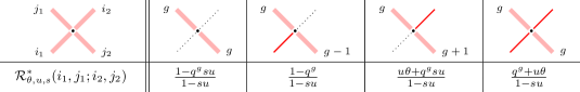
Figure 25. The cross vertex weights $\mathcal{R}^{*}_{\theta,u,s}(i_{1},j_{1};i_{2},j_{2})$, $i_{1},i_{2}\in\left\{0,1\right\}$, $j_{1},j_{2}\in\mathbb{Z}_{\geq 0}$.

A.4. Scaled geometric specialization

The scaled geometric specialization of the general fused weight $w^{(J)}_{u,s}$ is given by setting $u=-\epsilon\alpha$, $q^{J}=1/\epsilon$ and taking the limit $\epsilon\to 0$. Analogously we can specialize the dual weight $w^{*,(I)}_{v,s}$ taking $v=-\beta\epsilon$, $q^{I}=1/\epsilon$ and again $\epsilon\to 0$. In this case the expessions (A.3), (A.5) simplify:

$$\widetilde{w}_{\alpha,s}(i_{1},j_{1};i_{2},j_{2})=\mathbf{1}_{i_{1}+j_{1}=i_{2}+j_{2}}\,\frac{(-\alpha/s)^{i_{1}}(-s)^{j_{2}}(q;q)_{j_{1}}}{(q;q)_{i_{1}}(q;q)_{j_{2}}}\,{}_{3}\overline{\phi}_{2}\left(\begin{minipage}{71.13188pt} \centering{$q^{-i_{1}};q^{-i_{2}},-s\alpha$} \\ \centering{$s^{2},q^{1+j_{2}-i_{1}}$} \@add@centering\@add@centering\end{minipage}\Big{|}\,q,-\frac{sq^{1+i_{2}+j_{2}}}{\alpha}\right),$$ (A.15)

and

$$\widetilde{w}_{\alpha,s}\biggl{(}\leavevmode\hbox to40.64pt{\vbox to33.73pt{\text{[drawing]}}}\biggr{)}\,=\frac{\alpha^{k}}{(q;q)_{k}}. \infty \infty k \infty \infty k$$ (A.16)

The dual weights $\widetilde{w}^{*}_{\beta,s}$ are defined in the usual way as in (3.8).

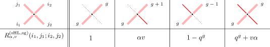
Figure 26. The cross vertex weight $R^{(\mathrm{sHL,sg})}_{\alpha,v}(i_{1},j_{1};i_{2},j_{2})$, $j_{1},j_{2}\in\{0,1\}$, $i_{1},i_{2}\in\mathbb{Z}_{\geq 0}$.

We also consider the scaled geometric specialization of the fused cross weight $R^{(I,J)}$, in this case in the parameters $v,q^{I}$, defining

$$\begin{split}R_{u,\beta}^{(\mathrm{sg},J)}(i_{1},j_{1};i_{2},j_{2})&=\mathbf{1}_{i_{2}+j_{1}=i_{1}+j_{2}}\,\frac{(-uq^{J}\beta)^{i_{2}}(q^{-J};q)_{i_{2}}}{(q;q)_{i_{2}}(q^{-J};q)_{i_{1}}}\,{}_{3}\overline{\phi}_{2}\left(\begin{minipage}{71.13188pt} \centering{$q^{-i_{1}};q^{-i_{2}},-u\beta$} \\ \centering{$q^{-J},q^{1+j_{2}-i_{2}}$} \@add@centering\@add@centering\end{minipage}\Big{|}\,q,-\frac{q^{1+i_{1}+j_{2}}}{uq^{J}\beta}\right).\end{split}$$ (A.17)

The scaled geometric specialization of $R^{(I,J)}$ in the parameters $u,q^{J}$ can be derived from (A.17) using the symmetry (A.9) and it is

$$R^{(I,\mathrm{sg})}_{\alpha,v}(i_{1},j_{1};i_{2},j_{2})=R^{(\mathrm{sg},I)}_{v,\alpha}(j_{1},i_{1};j_{2},i_{2}).$$ (A.18)

Further degenerations of $R^{(I,\mathrm{sg})}_{\alpha,v}$ involve specializations of parameters $v,q^{I}$ in one of the three cases, $\mathrm{sHL}(v)$ (which is simply $I=1$), $\mathrm{sqW}(\theta)$, or $\textrm{sg}(\beta)$. These cross vertex weights are given, respectively, in Figure 26 and below:

$$R^{\mathrm{(sqW,sg)}}_{\alpha,\theta}(i_{1},j_{1};i_{2},j_{2}) =\mathbf{1}_{i_{2}+j_{1}=i_{1}+j_{2}}\,\frac{(\alpha\theta)^{j_{2}}(-s/\theta;q)_{j_{2}}}{(q;q)_{j_{2}}(-s/\theta;q)_{j_{1}}}\,{}_{3}\overline{\phi}_{2}\left(\begin{minipage}{71.13188pt} \centering{$q^{-j_{1}};q^{-j_{2}},-s\alpha$} \\ \centering{$-s/\theta,q^{1+i_{1}-j_{1}}$} \@add@centering\@add@centering\end{minipage}\Big{|}\,q,\frac{q^{1+j_{1}+i_{2}}}{\alpha\theta}\right),$$ (A.19)

$$R^{\mathrm{(sg,sg)}}_{\alpha,\beta}(i_{1},j_{1};i_{2},j_{2}) =\mathbf{1}_{i_{2}+j_{1}=i_{1}+j_{2}}\,\frac{(\alpha\beta)^{j_{2}}}{(q;q)_{j_{2}}}\,{}_{2}\overline{\phi}_{1}\left(\begin{minipage}{56.9055pt} \centering{$q^{-j_{1}};q^{-j_{2}}$} \\ \centering{$q^{1+i_{1}-j_{1}}$} \@add@centering\@add@centering\end{minipage}\Big{|}\,q,\frac{q^{1+j_{1}+i_{2}}}{\alpha\beta}\right).$$ (A.20)

These cross vertex weights enter a number of Yang-Baxter equations which are specializations of the general fused one (A.8):

Proposition A.7.

We have the following Yang-Baxter equations:

$$\begin{split}&\sum_{k_{1},k_{2},k_{3}}R^{\mathrm{(sHL,sg)}}_{\alpha,v}(i_{2},i_{1};k_{2},k_{1})\,w^{*}_{v,s}(i_{3},k_{1};k_{3},j_{1})\,\widetilde{w}_{\alpha,s}(k_{3},k_{2};j_{3},j_{2})\\ &\hskip 50.0pt=\sum_{k_{1},k_{2},k_{3}}\,w^{*}_{v,s}(k_{3},i_{1};j_{3},k_{1})\,\widetilde{w}_{\alpha,s}(i_{3},i_{2};k_{3},k_{2})\,R^{\mathrm{(sHL,sg)}}_{\alpha,v}(k_{2},k_{1};j_{2},j_{1});\end{split}$$ (A.21)

$$\begin{split}&\sum_{k_{1},k_{2},k_{3}}R^{\mathrm{(sqW,sg)}}_{\alpha,\theta}(i_{2},i_{1};k_{2},k_{1})\,W^{*}_{\theta,s}(i_{3},k_{1};k_{3},j_{1})\,\widetilde{w}_{\alpha,s}(k_{3},k_{2};j_{3},j_{2})\\ &\hskip 50.0pt=\sum_{k_{1},k_{2},k_{3}}\,W^{*}_{\theta,s}(k_{3},i_{1};j_{3},k_{1})\,\widetilde{w}_{\alpha,s}(i_{3},i_{2};k_{3},k_{2})\,R^{\mathrm{(sqW,sg)}}_{\alpha,\theta}(k_{2},k_{1};j_{2},j_{1});\end{split}$$ (A.22)

$$\begin{split}&\sum_{k_{1},k_{2},k_{3}}R^{\mathrm{(sg,sg)}}_{\alpha,\beta}(i_{2},i_{1};k_{2},k_{1})\,\widetilde{w}^{*}_{\beta,s}(i_{3},k_{1};k_{3},j_{1})\,\widetilde{w}_{\alpha,s}(k_{3},k_{2};j_{3},j_{2})\\ &\hskip 50.0pt=\sum_{k_{1},k_{2},k_{3}}\widetilde{w}^{*}_{\beta,s}(k_{3},i_{1};j_{3},k_{1})\,\widetilde{w}_{\alpha,s}(i_{3},i_{2};k_{3},k_{2})\,R^{\mathrm{(sg,sg)}}_{\alpha,\beta}(k_{2},k_{1};j_{2},j_{1}).\end{split}$$ (A.23)

Dual cases of (A.21),(A.22),(A.23) obtained swapping the specializations are easily derived making use of the symmetry of the cross weight (A.18).

In Section 3, Cauchy Identities for spin Hall-Littlewood and spin $q$-Whittaker functions were stated as corollaries of the Yang-Baxter equations given in this appendix. In particular, the emergence of the prefactors in the right-hand sides of all the skew Cauchy identities can be traced to Proposition A.5.

A.5. Nonnegativity of terms in the Yang-Baxter equations

Here we list conditions which are sufficient for the nonnegativity of all terms in both sides of the Yang-Baxter equations described in the previous parts of this Appendix. We will not discuss which of these assumptions are necessary. If the terms are nonnegative, then by Proposition 6.4 a stochastic bijectivization of the Yang-Baxter equation exists. We assume that $s\in(-1,0)$ and $q\in(0,1)$ throughout the rest of the subsection.

First, the weights $w_{u,s}$ and $w^{*}_{v,s}$ given in Figure 6 and Figure 8 are nonnegative for $u,v\in[0,1]$. The cross vertex weights $r_{u/v}$ from Figure 21 are nonnegative when in addition $u<v$. Thus,

All summands in both sides of the Yang-Baxter equation (A.1) containing the weights $$w_{u,s},w_{v,s} r_{u/v} 0\leq u<v\leq 1$$, and are nonnegative if .

Next, the cross vertex weights $R_{uv}$ from Figure 23 are nonnegative when $0\leq uv<1$. Therefore,

All summands in both sides of the Yang-Baxter equation (A.2) containing the weights $$w_{u,s},w^{*}_{v,s} R_{uv} u,v\in[0,1) (u,v)\in\mathsf{Adm}$$, and are nonnegative if . This in fact implies that for the sHL/sHL skew Cauchy structure (Definition 3.5).

Let us now turn to the spin $q$-Whittaker weights. The weights $W_{\xi,s}$ and $W^{*}_{\theta,s}$ are nonnegative when $\xi,\theta\in[-s,-s^{-1}]$. The weights $\mathcal{R}_{\xi,v,s}$ and $\mathcal{R}^{*}_{\theta,u,s}$ from Figures 25 and 24 are nonnegative when $u,v\in[0,1)$ and $\xi,\theta\in[-s,-s^{-1}]$. Thus, we have

All summands in both sides of the Yang-Baxter equation (A.11) containing the weights $$W_{\xi,s},w^{*}_{v,s} \mathcal{R}_{\xi,v,s} v\in[0,1) \xi\in[-s,-s^{-1}] u\in[0,1),\theta\in[-s,-s^{-1}]$$, and are nonnegative if and . Similarly, the summands in (A.12) are nonnegative for .

Further, let us consider (A.13) containing $W_{\xi,s}$, $W_{\theta,s}^{*}$, and the non-factorized weights $\mathbb{R}_{\xi,\theta,s}$ (A.14). Their nonnegativity is not as straightforward, and requires an additional restriction on the parameters $s$ and $q$:

Proposition A.8.

For $\xi,\theta\in[-s,-s^{-1}]$, $q\in(0,1)$ and $s\in[-\sqrt{q},0)$, we have

$$\mathbb{R}_{\xi,\theta,s}(i_{1},j_{1};i_{2},j_{2})\geq 0\qquad\text{for all $i_{1},j_{1},i_{2},j_{2}\in\mathbb{Z}_{\geq 0}$}.$$

The proof of this proposition is similar to [CMP18, Proposition 3.1], with an additional simplification in the second case due to a symmetry of $\mathbb{R}_{\xi,\theta,s}$.

Proof of Proposition A.8.

Throughout the proof we will assume that $i_{2}+j_{1}=i_{1}+j_{2}$. We need to show that

$$\frac{s^{j_{2}}(-\theta q^{1-i_{1}-j_{2}}/s;q)_{i_{2}}}{(-q/(s\xi);q)_{i_{1}-j_{1}}}\,{}_{4}{\phi}_{3}\left(\begin{minipage}{119.50148pt} \centering{$q^{-i_{2}},-\frac{q}{s\xi},-s\theta,q^{-i_{1}}$} \\ \centering{$-\frac{\theta}{s}q^{1-i_{1}-j_{2}},-\frac{s}{\xi},q^{1+j_{2}-i_{2}}$} \@add@centering\@add@centering\end{minipage}\bigg{|}\,q,q\right)\geq 0.$$ (A.24)

Here we used (1.4) to get to the usual $q$-hypergeometric function, and also the fact that the remaining prefactor in $\mathbb{R}_{\xi,\theta,s}$ having the form

$$\frac{q^{i_{2}i_{1}+\frac{1}{2}j_{2}(j_{2}-1)}\xi^{j_{2}}(q;q)_{j_{1}}(-s/\xi;q)_{i_{2}}(q^{1+j_{2}-i_{2}};q)_{i_{2}}}{(s^{2};q)_{j_{1}+i_{2}}(q;q)_{j_{2}}(q;q)_{i_{2}}}$$

is nonnegative under our parameter restrictions in a straightforward way.

We will use Watson’s transformation formula [GR04, (III.19)]

$${{}_{4}}\phi_{3}\left(\begin{minipage}{56.9055pt} \centering{$q^{-n},a,b,c$} \\ \centering{$d,e,f$} \@add@centering\@add@centering\end{minipage}\bigg{|}\,q,q\right)=\frac{(d/b;q)_{n}(d/c;q)_{n}}{(d;q)_{n}(d/(bc);q)_{n}}\,{{}_{8}}\phi_{7}\left(\begin{minipage}{147.95424pt} \centering{$q^{-n},\sigma,q\sigma^{1/2},-q\sigma^{1/2},\frac{f}{a},\frac{e}{a},b,c$} \\ \centering{$\sigma^{1/2},-\sigma^{1/2},e,f,\frac{ef}{ab},\frac{ef}{ac},\frac{efq^{n}}{a}$} \@add@centering\@add@centering\end{minipage}\bigg{|}\,q,\frac{efq^{n}}{bc}\right),$$ (A.25)

where $def=abcq^{1-n}$ and $\sigma=ef/aq$.

Case 1. When $i_{2}\leq j_{2}$, we apply (A.25) to (A.24) with $n=i_{2}$. The prefactor in (A.25) combined with the one from (A.24) becomes

$$\frac{s^{j_{2}}}{(-q/(s\xi);q)_{i_{1}-j_{1}}}\frac{(q^{1-i_{1}-j_{2}}/s^{2};q)_{i_{2}}(-\theta q^{1-j_{2}}/s;q)_{i_{2}}}{(q^{1-j_{2}}/s^{2};q)_{i_{2}}}.$$

We have

$$\frac{(q^{1-i_{1}-j_{2}}/s^{2};q)_{i_{2}}}{(q^{1-j_{2}}/s^{2};q)_{i_{2}}}=\prod_{m=1}^{i_{2}}\frac{q^{m-j_{2}}q^{-i_{1}}-s^{2}}{q^{m-j_{2}}-s^{2}}\geq 0,$$

since $m-j_{2}\leq 0$ in the product. We also have

$$\frac{s^{j_{2}}(-\theta q^{1-j_{2}}/s;q)_{i_{2}}}{(-q/(s\xi);q)_{i_{1}-j_{1}}}=s^{j_{2}}\prod_{k=1}^{i_{2}}\left(1+\frac{\theta}{s}\,q^{k-j_{2}}\right)\prod_{m=1}^{j_{2}-i_{2}}\left(1+\frac{q^{1-m}}{s\xi}\right)\geq 0,$$

since all factors above (including $s^{j_{2}}$) are nonpositive, and there is a total of $2j_{2}$ of them.

The $q$-hypergeometric function after applying (A.25) to (A.24) takes the form

$${{}_{8}}\phi_{7}\left(\begin{minipage}{233.3125pt} \centering{$q^{-i_{2}},\sigma,q\sigma^{1/2},-q\sigma^{1/2},-s\xi q^{j_{2}-i_{2}},\frac{s^{2}}{q},-s\theta,q^{-i_{1}}$} \\ \centering{$\sigma^{1/2},-\sigma^{1/2},-\frac{s}{\xi},q^{1+j_{2}-i_{2}},-\frac{s}{\theta}q^{j_{2}-i_{2}},s^{2}q^{j_{1}},s^{2}q^{j_{2}}$} \@add@centering\@add@centering\end{minipage}\bigg{|}\,q,\frac{q^{i_{1}+j_{2}+1}}{\xi\theta}\right),$$

with $\sigma=s^{2}q^{j_{2}-i_{2}-1}\in(0,1)$ because $s^{2}\leq q$. One readily sees that each summand in this (terminating) $q$-hypergeometric series is nonnegative. Indeed, the only negative signs may come from $(q^{-i_{2}};q)_{k}$, $(q^{-i_{1}};q)_{k}$, and $(s^{2}q^{-1};q)_{k}$. However, the product of the former two factors is always nonnegative, and $(s^{2}q^{-1};q)_{k}\geq 0$ also due to our additional parameter restriction $s^{2}\leq q$. This implies the nonnegativity of $\mathbb{R}_{\xi,\theta,s}(i_{1},j_{1};i_{2},j_{2})$ when $i_{2}\leq j_{2}$.

Case 2. When $i_{2}>j_{2}$, the claim follows due to the symmetry of $\mathbb{R}_{\xi,\theta,s}$. Namely, by means of Remark A.4, we have

$$\mathbb{R}_{\xi,\theta,s}(i_{1},j_{1};i_{2},j_{2})=\mathbb{R}_{\theta,\xi,s}(j_{1},i_{1};j_{2},i_{2})$$

for all $i_{1},j_{1},i_{2},j_{2}\in\mathbb{Z}_{\geq 0}$. This completes the proof. ∎

Proposition A.8 implies that

All summands in both sides of the Yang-Baxter equation (A.13) containing the weights $$W_{\xi,s},W^{*}_{\theta,s} \mathbb{R}_{\xi,\theta,s} \xi,\theta\in[-s,-s^{-1}] q\in(0,1) s\in[-\sqrt{q},0)$$, and are nonnegative if , , and .

Finally, we address the nonnegativity of terms of the Yang-Baxter equations involving scaled geometric specializations from Proposition A.7.

Proposition A.9.

For $\alpha\in[0,-s^{-1}]$, $q\in(0,1)$ and $s\in(-1,0)$ we have

$$\widetilde{w}_{\alpha,s}(i_{1},j_{1};i_{2},j_{2})\geq 0\qquad\text{for all }i_{1},j_{1},i_{2},j_{2}\in\mathbb{Z}_{\geq 0}.$$

Proof.

Under our assumptions the prefactor

$$\frac{(-\alpha/s)^{i_{1}}(-s)^{j_{2}}(q;q)_{j_{1}}}{(q;q)_{i_{1}}(q;q)_{j_{2}}}$$

is nonnegative. To check the remaining term, we write down the generic summand of the terminating $q$-hypergeometric series as (cf. (1.4)):

$$\left(\frac{-sq^{1+j_{2}+i_{2}}}{\alpha}\right)^{k}\frac{(q^{-i_{1}};q)_{k}}{(q;q)_{k}}(q^{-i_{2}};q)_{k}(-s\alpha;q)_{k}(s^{2}q^{k};q)_{i_{1}-k}(q^{1+j_{2}-i_{1}+k};q)_{i_{1}-k},$$

where $k=0,\dots,i_{1}$. The leading monomial term, along with $(s^{2}q^{k};q)_{i_{1}-k}$ and $(q;q)_{k}$ are always nonnegative. The $q$-Pochhammer symbols of $q^{-i_{1}}$ and $q^{-i_{2}}$ either vanish, or they both carry a sign $(-1)^{k}$, so that their contribution is nonnegative too. Next, $(q^{1+j_{2}-i_{1}+k};q)_{i_{1}-k}$ is either nonnegative if $1+j_{2}-i_{1}+k>0$, or vanishes if $1+j_{2}-i_{1}+k\leq 0$ (in the latter case, the last term of the product has power $j_{2}\geq 0$, which means that that product passes through $1-q^{0}=0$). Finally, $(-s\alpha;q)_{k}\geq 0$ because $\alpha\leq-s^{-1}$. ∎

Proposition A.9 and the explicit form of $R^{(\mathrm{sHL,sg})}_{\alpha,v}$ (Figure 26) implies that

All summands in both sides of the Yang-Baxter equation (A.21) containing the weights $$\widetilde{w}_{\alpha,s},w^{*}_{v,s} R^{(\mathrm{sHL,sg})}_{\alpha,v} \alpha\in[0,-s^{-1}] v\in[0,1)$$, and are nonnegative if , .

In order to demonstrate the nonnegativity of (A.22) we consider the corresponding cross vertex weight:

Proposition A.10.

For $\alpha\in[0,-s^{-1}]$ and $\theta\in[-s,-s^{-1}]$, we have

$$R^{(\mathrm{sqW,sg})}_{\alpha,\theta}(i_{1},j_{1};i_{2},j_{2})\geq 0\qquad\text{for all }i_{1},j_{1},i_{2},j_{2}\in\mathbb{Z}_{\geq 0}.$$

Proof.

Assume first that $\theta>-s$. In (A.19), the factors outside ${}_{3}\overline{\phi}_{2}$ are nonnegative. In the expansion of ${}_{3}\overline{\phi}_{2}$ using (1.4), one readily sees that all terms are nonnegative similarly to the proof of Proposition A.9 above (here we use the fact that $-s\alpha$ and $-s/\theta$ are less than 1 because of our assumptions).

We can now take the limit $\theta\to-s$ and show that the weight $R^{(\mathrm{sqW,sg})}$ survives this transition. To do so, expand ${}_{3}\overline{\phi}_{2}$ using (1.4), and collect terms containing $-s/\theta$:

$$\frac{(-s/\theta;q)_{j_{2}}(-q^{k}s/\theta;q)_{j_{1}-k}}{(-s/\theta;q)_{j_{1}}}=(-q^{k}s/\theta;q)_{j_{2}-k},$$

with $k=0,\dots,\min(j_{1},j_{2})$. The last expression is nonsingular at $\theta=-s$, and is nonnegative. ∎

Therefore,

All summands in both sides of the Yang-Baxter equation (A.22) containing $$\widetilde{w}_{\alpha,s},W^{*}_{\theta,s} R^{(\mathrm{sqW,sg})}_{\alpha,\theta} \alpha\in[0,-s^{-1}] \theta\in[-s,-s^{-1}]$$, and are nonnegative if , .

We come now to the last Yang-Baxter equation we stated (A.23), in which one readily sees (similarly to Propositions A.9 and A.10 above) that $R^{(\mathrm{sg,sg})}_{\alpha,\beta}$ is nonnegative when $0\leq\alpha,\beta\leq-s^{-1}$. Therefore,

All summands in both sides of the Yang-Baxter equation (A.23) containing $$\widetilde{w}_{\alpha,s},\widetilde{w}^{*}_{\beta,s} R^{(\mathrm{sg,sg})}_{\alpha,\beta} \alpha,\beta\in[0,-s^{-1}]$$, and are nonnegative if .

References

- [Agg18] A. Aggarwal “Current Fluctuations of the Stationary ASEP and Six-Vertex Model” arXiv:1608.04726 [math.PR] In Duke Math J. 167.2, 2018, pp. 269–384
- [ABB18] A. Aggarwal, A. Borodin and A. Bufetov “Stochasticization of Solutions to the Yang-Baxter Equation” arXiv:1810.04299 [math.PR] In arXiv preprint, 2018
- [BDJ99] J. Baik, P. Deift and K. Johansson “On the distribution of the length of the longest increasing subsequence of random permutations” arXiv:math/9810105 [math.CO] In Jour. AMS 12.4 American Mathematical Society, 1999, pp. 1119–1178
- [BBO05] P. Biane, P. Bougerol and N. O’Connell “Littelmann paths and brownian paths” arXiv:math/0403171 [math.RT] In Duke J. Math. 130.1, 2005, pp. 127–167
- [Bor10] Folkmar Bornemann “On the numerical evaluation of Fredholm determinants” arXiv:0804.2543 [math.NA] In Math. Comp. 79.270, 2010, pp. 871–915
- [Bor11] A. Borodin “Schur dynamics of the Schur processes” arXiv:1001.3442 [math.CO] In Adv. Math. 228.4, 2011, pp. 2268–2291
- [Bor17] A. Borodin “On a family of symmetric rational functions” arXiv:1410.0976 [math.CO] In Adv. Math. 306, 2017, pp. 973–1018 eprint: 1410.0976
- [BBW16] A. Borodin, A. Bufetov and M. Wheeler “Between the stochastic six vertex model and Hall-Littlewood processes” arXiv:1611.09486 [math.PR] In arXiv preprint, 2016
- [BC14] A. Borodin and I. Corwin “Macdonald processes” arXiv:1111.4408 [math.PR] In Probab. Theory Relat. Fields 158, 2014, pp. 225–400
- [BC15] A. Borodin and I. Corwin “Discrete time q-TASEPs” arXiv:1305.2972 [math.PR] In Int. Math. Res. Notices 2015.2, 2015, pp. 499–537
- [BCFV15] A. Borodin, I. Corwin, P. Ferrari and B. Veto “Height fluctuations for the stationary KPZ equation” arXiv:1407.6977 [math.PR] In Mathematical Physics, Analysis and Geometry 18.1, 2015, pp. 1–95
- [BCG16] A. Borodin, I. Corwin and V. Gorin “Stochastic six-vertex model” arXiv:1407.6729 [math.PR] In Duke J. Math. 165.3, 2016, pp. 563–624
- [BCPS15] A. Borodin, I. Corwin, L. Petrov and T. Sasamoto “Spectral theory for interacting particle systems solvable by coordinate Bethe ansatz” In Commun. Math. Phys. 339.3, 2015, pp. 1167–1245
- [BCS14] A. Borodin, I. Corwin and T. Sasamoto “From duality to determinants for q-TASEP and ASEP” arXiv:1207.5035 [math.PR] In Ann. Probab. 42.6, 2014, pp. 2314–2382
- [BF14] A. Borodin and P. Ferrari “Anisotropic growth of random surfaces in 2+1 dimensions” arXiv:0804.3035 [math-ph] In Commun. Math. Phys. 325, 2014, pp. 603–684
- [BP16] A. Borodin and L. Petrov “Lectures on Integrable probability: Stochastic vertex models and symmetric functions” arXiv:1605.01349 [math.PR] In Lecture Notes of the Les Houches Summer School 104, 2016 eprint: 1605.01349
- [BP16a] A. Borodin and L. Petrov “Nearest neighbor Markov dynamics on Macdonald processes” arXiv:1305.5501 [math.PR] In Adv. Math. 300, 2016, pp. 71–155 eprint: 1305.5501
- [BP18] A. Borodin and L. Petrov “Higher spin six vertex model and symmetric rational functions” arXiv:1601.05770 [math.PR] In Selecta Math. 24.2, 2018, pp. 751–874 eprint: 1601.05770
- [BP18a] A. Borodin and L. Petrov “Inhomogeneous exponential jump model” arXiv:1703.03857 [math.PR] In Probab. Theory Relat. Fields 172, 2018, pp. 323–385 eprint: 1703.03857
- [BR05] A. Borodin and E.M. Rains “Eynard–Mehta theorem, Schur process, and their Pfaffian analogs” arXiv:math-ph/0409059 In J. Stat. Phys 121.3 Springer, 2005, pp. 291–317
- [BW17] A. Borodin and M. Wheeler “Spin -Whittaker polynomials” arXiv:1701.06292 [math.CO] In arXiv preprint, 2017
- [BM18] A. Bufetov and K. Matveev “Hall-Littlewood RSK field” arXiv:1705.07169 [math.PR] In Selecta Math. 24.5, 2018, pp. 4839–4884
- [BP15] A. Bufetov and L. Petrov “Law of Large Numbers for Infinite Random Matrices over a Finite Field” arXiv:1402.1772 [math.PR] In Selecta Math. 21.4, 2015, pp. 1271–1338 eprint: 1402.1772
- [BP17] A. Bufetov and L. Petrov “Yang-Baxter field for spin Hall-Littlewood symmetric functions” arXiv:1712.04584 [math.PR] In arXiv preprint, 2017 eprint: 1712.04584
- [Chh13] R. Chhaibi “Littelmann path model for geometric crystals, Whittaker functions on Lie groups and Brownian motion” arXiv:1302.0902 [math.PR], 2013
- [Cor14] I. Corwin “The -Hahn Boson process and -Hahn TASEP” arXiv:1401.3321 [math.PR] In Int. Math. Res. Notices, 2014
- [CMP18] I. Corwin, K. Matveev and L. Petrov “The q-Hahn PushTASEP” arXiv:1811.06475 [math.PR]. Intern. Math. Research Notices, to appear In arXiv preprint, 2018
- [COSZ14] I. Corwin, N. O’Connell, T. Seppäläinen and N. Zygouras “Tropical Combinatorics and Whittaker functions” arXiv:1110.3489 [math.PR] In Duke J. Math. 163.3, 2014, pp. 513–563
- [CP16] I. Corwin and L. Petrov “Stochastic higher spin vertex models on the line” arXiv:1502.07374 [math.PR] In Commun. Math. Phys. 343.2, 2016, pp. 651–700 eprint: 1502.07374
- [DLSS91] B. Derrida, J. Lebowitz, E. Speer and H. Spohn “Dynamics of an anchored Toom interface” In J. Phys. A 24.20, 1991, pp. 4805
- [DF90] P. Diaconis and J.A. Fill “Strong Stationary Times via a New Form of Duality” In Ann. Probab. 18, 1990, pp. 1483–1522
- [Dim18] E. Dimitrov “Six-vertex Models and the GUE-corners Process” arXiv:1610.06893 [math.PR] In Intern. Math. Research Notices, 2018, pp. rny072 DOI: 10.1093/imrn/rny072
- [GGW17] A. Garbali, J. Gier and M. Wheeler “A new generalisation of Macdonald polynomials” arXiv:1605.07200 [math-ph] In Comm. Math. Phys 352.2, 2017, pp. 773–804
- [GR04] G. Gasper and M. Rahman “Basic hypergeometric series” Cambridge University Press, 2004
- [GM14] G. Gimmett and I. Manolescu “Bond percolation on isoradial graphs: criticality and universality” arXiv:1204.0505 [math.PR] In Bond percolation on isoradial graphs: criticality and universality 159.1-2, 2014, pp. 273–327
- [GS92] L.-H. Gwa and H. Spohn “Six-vertex model, roughened surfaces, and an asymmetric spin Hamiltonian” In Phys. Rev. Lett. 68.6, 1992, pp. 725–728
- [IMS19] T. Imamura, M. Mucciconi and T. Sasamoto “Stationary Higher Spin Six Vertex Model and -Whittaker measure” arXiv:1901.08381 [math-ph] In arXiv preprint, 2019
- [Joh00] K. Johansson “Shape fluctuations and random matrices” arXiv:math/9903134 [math.CO] In Commun. Math. Phys. 209.2 Springer, 2000, pp. 437–476
- [KRS81] P. Kulish, N. Reshetikhin and E. Sklyanin “Yang-Baxter equation and representation theory: I” In Letters in Mathematical Physics 5.5 Springer, 1981, pp. 393–403
- [Mac95] I.G. Macdonald “Symmetric functions and Hall polynomials” Oxford University Press, 1995
- [Man14] V. Mangazeev “On the Yang–Baxter equation for the six-vertex model” arXiv:1401.6494 [math-ph] In Nuclear Physics B 882, 2014, pp. 70–96
- [MP17] K. Matveev and L. Petrov “-randomized Robinson–Schensted–Knuth correspondences and random polymers” arXiv:1504.00666 [math.PR] In Annales de l’IHP D 4.1, 2017, pp. 1–123 eprint: 1504.00666
- [O’C03] N. O’Connell “A path-transformation for random walks and the Robinson-Schensted correspondence” In Trans. AMS 355.9, 2003, pp. 3669–3697
- [O’C03a] N. O’Connell “Conditioned random walks and the RSK correspondence” In J. Phys. A 36.12, 2003, pp. 3049–3066
- [O’C12] N. O’Connell “Directed polymers and the quantum Toda lattice” arXiv:0910.0069 [math.PR] In Ann. Probab. 40.2, 2012, pp. 437–458
- [OP13] N. O’Connell and Y. Pei “A q-weighted version of the Robinson-Schensted algorithm” arXiv:1212.6716 [math.CO] In Electron. J. Probab. 18.95, 2013, pp. 1–25
- [OSZ14] N. O’Connell, T. Seppäläinen and N. Zygouras “Geometric RSK correspondence, Whittaker functions and symmetrized random polymers” arXiv:1110.3489 [math.PR] In Invent. Math. 197, 2014, pp. 361–416
- [Oko01] A. Okounkov “Infinite wedge and random partitions” arXiv:math/9907127 [math.RT] In Selecta Math. 7.1 Springer, 2001, pp. 57–81
- [OR03] A. Okounkov and N. Reshetikhin “Correlation function of Schur process with application to local geometry of a random 3-dimensional Young diagram” arXiv:math/0107056 [math.CO] In Jour. AMS 16.3 American Mathematical Society, 2003, pp. 581–603
- [OP17] D. Orr and L. Petrov “Stochastic Higher Spin Six Vertex Model and -TASEPs” In Adv. Math. 317, 2017, pp. 473–525 DOI: 10.1016/j.aim.2017.07.003
- [Pov13] A. Povolotsky “On integrability of zero-range chipping models with factorized steady state” arXiv:1308.3250 [math-ph] In J. Phys. A 46, 2013, pp. 465205
- [Spi70] F. Spitzer “Interaction of Markov processes” In Adv. Math. 5.2, 1970, pp. 246–290
- [Spo15] A. Sportiello “Personal communication”, 2015
- [VK86] A. Vershik and S. Kerov “The characters of the Infinite Symmetric Group and Probability Properties of the Robinson-Shensted-Knuth algorithm” In SIAM J. Alg. Disc. Math. 7.1, 1986, pp. 116–124
- [WW09] J. Warren and P. Windridge “Some examples of dynamics for Gelfand-Tsetlin patterns” arXiv:0812.0022 [math.PR] In Electron. J. Probab. 14 The Institute of Mathematical Statisticsthe Bernoulli Society, 2009, pp. 1745–1769
- [WZJ16] M. Wheeler and P. Zinn-Justin “Refined Cauchy/Littlewood identities and six-vertex model partition functions: III. Deformed bosons” arXiv:1508.02236 [math-ph] In Adv. Math 299, 2016, pp. 543–600