Phase behavior of flexible and semiflexible polymers in solvents of varying quality

Abstract

The interplay of nematic order and phase separation in solutions of semiflexible polymers in solvents of variable quality is investigated by density functional theory (DFT) and molecular dynamics (MD) simulations. We studied coarse-grained models, with a bond-angle potential to control chain stiffness, for chain lengths comparable to the persistence length of the chains. We varied both the density of the monomeric units and the effective temperature that controls the quality of the implicit solvent. For very stiff chains only a single transition from an isotropic fluid to a nematic is found, with a phase diagram of “swan-neck” topology. For less stiff chains, however, also unmixing between isotropic fluids of different concentration, ending in a critical point, occurs for temperatures above a triple point. The associated critical behavior is examined in the MD simulations and found compatible with Ising universality. Apart from this critical behavior, DFT calculations agree qualitatively with the MD simulations.

I Introduction

Semiflexible polymers in solutions occur in many different contexts, from materials science to biophysics and biochemistry. Concentrated solutions are expected to exhibit liquid crystalline order, and hence may exhibit interesting material properties.Ciferri, Krigbaum, and Meyer (1982); Ciferri (1983); Donald, Windle, and Hanna (2006) Biological macromolecules often show considerable stiffness, for example, double-stranded (ds) DNA, filamentous (F) actin, phospholipids, etc., and this stiffness is relevant for their functions in cells and tissues.Brown and Wolsen (1979); Köster et al. (2015) Under good solvent conditions, the effective interactions between the monomeric units of these semiflexible polymers are purely repulsive. With increasing concentration of the lyotropic solution a phase transition from the isotropic phase to a nematic phase occurs.Ciferri, Krigbaum, and Meyer (1982); Ciferri (1983); Donald, Windle, and Hanna (2006) Such systems have also been extensively studied by theory,Grosberg and Khokhlov (1981); Khokhlov and Semenov (1981, 1982a, 1982b); Odijk (1983); Khokhlov and Semenov (1985); Odijk (1985, 1986a, 1986b); Grosberg and Zhestkov (1986); Vroege and Odijk (1988); Shimada, Doi, and Okano (1988); Hentschke (1990); Taylor and Herzfeld (1990); Hentschke and Herzfeld (1991); DuPré and Yang (1991); Selinger and Bruinsma (1991a, b); Chen (1993); Sato and Teramoto (1994, 1996a, 1996b); Egorov, Milchev, and Binder (2016); Egorov et al. (2016); Milchev et al. (2018) which has been inspired by Onsager’s theoryOnsager (1949) for the isotropic-nematic transition in solutions of hard rods,Fraden (1995); Lekkerkerker and Tuinier (2011) and by computer simulations.Egorov, Milchev, and Binder (2016); Egorov et al. (2016); Milchev et al. (2018); Wilson and Allen (1993); Dijkstra and Frenkel (1995); Kamien and Grest (1997); Lyulin et al. (1998); Naderi and van der Schoot (2014); de Braaf et al. (2017)

For such lyotropic solutions, the phase behavior is solely dictated by the bending energy of the chains and the competition between their orientational and packing entropy. However, under many conditions of physical interest, solvent quality is an additional key parameter that needs to be taken into account as well.Lekkerkerker and Tuinier (2011); Yamakawa (1971); de Gennes (1979); Grosberg and Khokhlov (1994); Rubinstein and Colby (2003) For flexible polymers in solution at temperatures $T$ below the $\Theta$-temperature, $T_{\Theta}$, the phase separation into a dilute region coexisting with a more concentrated solution is a classical problem described in textbooks.Yamakawa (1971); de Gennes (1979); Grosberg and Khokhlov (1994); Rubinstein and Colby (2003) For flexible polymers at $T>T_{\Theta}$, increasing the polymer concentration causes a gradual crossover from swollen coils (radius of gyration, $R_{\rm g}$, scales with the contour length, $L$, as $R_{\rm g}\propto L^{3/5}$) to Gaussian coils ($R_{\rm g}\propto L^{1/2}$), but there is no phase transition whatsoever.

For semiflexible polymers, the theoretical description becomes much more challenging due to the coupling of translational and orientational degrees of freedom. Further, while for flexible polymers in dilute solution the coil structure is self-similar on all scales from the diameter of the monomeric units, $d$, to $R_{\rm g}$, for semiflexible polymers the persistence length, $\ell_{\rm p}$, presents an additional relevant length scale.Yamakawa (1971); Grosberg and Khokhlov (1994); Rubinstein and Colby (2003); Hsu, Paul, and Binder (2010) When $\ell_{\rm p}/d$ stays of order unity, only the coil radius is somewhat enhanced, i.e. $R_{\rm g}^{2}\approx L\ell_{\rm p}/3$ rather than $R_{\rm g}^{2}\approx Ld/6$ in very concentrated solutions. However, when $\ell_{\rm p}/d$ is large enough, the isotropic solution exhibits a (first order) phase transition to the nematic phase, with a two-phase coexistence region of the monomer density, $\rho$, in the solution from $\rho_{{}_{\rm I}}$ to $\rho_{{}_{\rm N}}$. For $L\gg\ell_{\rm p}$, both $\rho_{{}_{\rm I}}$ and $\rho_{{}_{\rm N}}$ scale as $\rho_{{}_{\rm I,N}}d^{3}\propto d/\ell_{\rm p}$ when $d/\ell_{\rm p}$ is very small, while for $L\approx\ell_{\rm p}$ a crossover to $\rho_{{}_{\rm I,N}}d^{3}\propto d/L$ occurs.Grosberg and Khokhlov (1981); Khokhlov and Semenov (1981, 1982a, 1982b); Odijk (1983); Khokhlov and Semenov (1985); Odijk (1985, 1986a, 1986b); Grosberg and Zhestkov (1986); Vroege and Odijk (1988); Chen (1993) The latter regime is the same as of hard rods in solution, and can be understood in terms of the orientation-dependent excluded volume between a pair of rods with regards to their second virial coefficient.Onsager (1949) Since for large enough $L$ (or $\ell_{\rm p}$, respectively) $\rho_{{}_{\rm I}}$ and $\rho_{{}_{\rm N}}$ are very small, such a treatment can be shown to be self-consistent.Lekkerkerker and Tuinier (2011)

However, when attractive interactions between the effective monomeric units of the rods (or semiflexible polymers, respectively) are present, the situation is different: whenever the attraction becomes strong enough to be noticeable, the second virial approximation becomes unreliable.van der Schoot and Odijk (1992) Van der Schoot and Odijkvan der Schoot and Odijk (1992) speculated that under some conditions for solutions of long rods with van der Waals attraction it could happen that macroscopic phase separation is prevented by the formation of finite aggregates (“bundles” of rods). However, explicit calculations were mostly restricted to rod-like particles modeled by spherocylinders where attraction is due to depletion forces caused by non-adsorbing ideal polymer coils whose radius controls the attraction range.Lekkerkerker and Stroobants (1994); Bolhuis and Frenkel (1997); Jungblut et al. (2007) Using scaled particle theoryCotter (1977) to account for attractions beyond the second virial approximation, phase diagrams were studied for both $L/d=3$ and $L/d=5$, and compared to Monte Carlo simulation results.Bolhuis and Frenkel (1997); Jungblut et al. (2007) For a large enough range of the attraction, phase separation within the isotropic phase occurs, followed by the isotropic-nematic transition (at larger densities). As expected, the theory is not quantitatively accurate: it predicts mean field critical behavior instead of the expected Ising like behaviorStanley (1971) for the isotropic-isotropic phase separation, but is inaccurate also outside the critical region. At this point, we recall that application of scaled particle theory to lyotropic solutions of semiflexible polymersSato and Teramoto (1994, 1996a, 1996b) was foundEgorov, Milchev, and Binder (2016); Egorov et al. (2016) to yield much less accurate results than density functional theory (DFT). Hence, we shall only compare the latter approach in the present work. While for very long spherocylinders also nematic-nematic phase separation has been predicted,Bolhuis and Frenkel (1997) this is not relevant for the systems that will be studied in the present paper, and also smectic and crystalline phasesBolhuis and Frenkel (1997); Milchev, Nikoubashman, and Binder (2019) will stay outside of consideration.

The aim of the present work is to elucidate the role of solvent quality on isotropic-nematic phase separation in solutions of semiflexible polymers where contour length $L$ and persistence length $\ell_{\rm p}$ are comparable (this regime is both of experimental interest and convenient for molecular dynamicsAllen and Tildesley (2017) simulations). We will study the interplay with phase separation in the isotropic solution, and for comparison we also consider phase separation for the same coarse-grained model in the limiting case of fully flexible chains, a problem that has already been studied in different context by related models (see, e.g., Refs. 53; 54). We note that the approach employed in this work is fundamentally different from the treatment of thermotropic liquid crystalline polymers, where an orientation-independent attraction (in terms of a Maier-Saupe like potentialde Gennes and Prost (1995)) is used.Daoulas, Rühle, and Kremer (2012); Gemünden and Daoulas (2015)

The rest of the manuscript is organized in the following way. In Section II, the studied models will be defined, and the applied methods briefly characterized. In Section III, we shall present predictions from DFT calculations augmented by adding isotropic attractive interactions to fully flexible (Section III.1) and semiflexible (Section III.2) chains. In selected cases, we shall compare the DFT results for the phase diagrams with corresponding MD results, demonstrating qualitative agreement. In Sec. III.3, additional results obtained from MD simulation are described, emphasizing the use of a newSiebert et al. (2018) version of finite size scaling using subsystems in an elongated simulation box geometry (technical aspects of this methodology are summarized in the Appendix). This method is useful for an accurate estimation of critical properties of the studied model system. Section IV then gives a final discussion of our results and presents an outlook for future work.

II Models and Methods

II.1 MD Simulations

To study the phase behavior of flexible and semiflexible polymers in solvents of varying quality, we use a coarse-grained bead-spring model, where each polymer consists of $N$ spherical monomeric units with diameter $\sigma$ and unit mass $m$. The solvent is modeled implicitly, and the solvent quality is incorporated into the effective monomer-monomer interaction

$$U_{\rm mm}(\lambda,r_{ij})=U_{\rm R}(r_{ij})+\lambda U_{\rm A}(r_{ij})$$ (1)

with $r_{ij}$ being the distance between particles $i$ and $j$. The parameter $\lambda$ controls the solvent quality, where $\lambda=0$ corresponds to good solvent conditions and the solvent quality worsens with increasing $\lambda$. The parameter $\lambda$ effectively plays the role of an inverse temperature, $T_{\rm eff}\equiv 1/\lambda$. The repulsive contribution, $U_{\rm R}(r_{ij})$, is modeled via

$$U_{\rm R}(r_{ij})=\begin{cases}U_{\rm LJ}(r_{ij})+\varepsilon&\text{for $r_{ij}\leq 2^{1/6}\sigma$\,}\\ 0&\text{for $r_{ij}>2^{1/6}\sigma$\,}\end{cases}$$ (2)

where $U_{\rm LJ}(r_{ij})=4\epsilon[(\sigma/r)^{12}-(\sigma/r)^{6}]$ is the standard Lennard-Jones (LJ) potential, and $\varepsilon$ is the strength of the potential. The attractive part of the monomer-monomer interaction, $U_{\rm A}(r_{ij})$, is defined as

$$U_{\rm A}(r_{ij})=\begin{cases}-\varepsilon&\text{for $r_{ij}\leq 2^{1/6}\sigma$\,}\\ U_{\rm LJ}(r_{ij})&\text{for $2^{1/6}\sigma<r_{ij}<r_{c}$\,}\end{cases}$$ (3)

with cutoff radius $r_{c}=4\sigma$.

Monomers are bonded via the finitely extensible nonlinear elastic (FENE) potential

$$U_{\rm FENE}(r_{ij})=-\frac{1}{2}kr_{0}^{2}\ln\left[1-\left(\frac{r_{ij}}{r_{0}}\right)^{2}\right].$$ (4)

Here, $r_{0}$ is the maximum bond extension which is set to $r_{0}=1.5\sigma$, and $k=30\varepsilon/\sigma^{2}$ is the spring constant.Grest and Kremer (1986) These values of the parameters impede unphysical bond crossing.

Bending stiffness for the polymers is incorporated via the potential

$$U_{\Theta}(\Theta_{ijk})=-\kappa[1-cos(\Theta_{ijk})],$$ (5)

where $\kappa$ controls the rigidity of a chain and $\Theta_{ijk}$ is the angle between two subsequent bond vectors, ${\bf r}_{ij}$ and ${\bf r}_{jk}$ connecting the monomers $i$, $j$ and $k$ of a chain. (An angle of $\Theta_{ijk}=0^{\circ}$ corresponds to the three monomers $i$, $j$, and $k$ in a line.) The persistence length of the polymers is defined as $\ell_{\rm p}=-\ell_{\rm b}/\ln\left\langle\cos\Theta_{ijk}\right\rangle$, with bond length $\ell_{\rm b}\approx 0.97\sigma$ for our choice of parameters. For $\kappa/(k_{\rm B}T)\gtrsim 2$, the expression for $\ell_{\rm p}$ can be approximated by $\ell_{\rm p}/\ell_{\rm b}\approx\kappa/(k_{\rm B}T)$.

We have opted to vary the effective tempeterature, $T_{\rm eff}$, instead of the thermodynamic temperature, $T$, as this approach only affects the strength of the attractive monomer-monomer contribution, while leaving the strength of the bond and bending interactions (and thus $\ell_{\rm p}$) unchanged. For a special case $\lambda=0$, our model becomes purely repulsive, which has been extensively studied in earlier work.Egorov, Milchev, and Binder (2016); Egorov et al. (2016); Milchev et al. (2018) There, the isotropic-nematic transition, hairpin formation, and elastic constants of the model were investigated for a range of chain lengths, $N$, and bending rigidities, $\kappa$.

All our MD simulations have been performed in the $\mathcal{N}VT$ ensemble using the HOOMD-blue software package.Anderson, Lorenz, and Travesset (2008); Glaser et al. (2015) The temperature of the system is kept constant at $T=1.0\varepsilon/k_{\rm B}$ using a Langevin thermostat with friction coefficient $\Gamma=0.25$, where $k_{\rm B}$ is Boltzmann’s constant. We set the simulation time step to $\Delta t=0.002\tau$, where $\tau=\sqrt{m\sigma^{2}/(k_{\rm B}T)}$ is the intrinsic MD unit of time. Unless stated otherwise explicitly, the simulations have been conducted in an elongated box, $\mathcal{L}_{x}=256\sigma$, $\mathcal{L}_{y}=64\sigma$ and $\mathcal{L}_{z}=32\sigma$, with periodic boundary conditions applied in all directions. The choice of such an elongated box is advantageous when state points are chosen that fall inside a two-phase coexistence region (see, e.g., Fig. 2 below). Then the high density phase is separated from the low density phase by two interfaces parallel to the $yz$-plane. Starting configurations were generated by regularly placing monomers along straight lines oriented along the $x$ or $y$-direction. We have verified that the “memory” of the initial configurations of the polymer chains is completely lost, and only included well equilibrated states for the averages taken.

II.2 Density Functional Theory

We construct the model for our DFT calculations analogous to the MD model described in Sec. II.1 above. The intramolecular potential characterizing the polymer chain can be written as a sum of three terms, i.e. the non-bonded segment-segment interaction potential, $U_{\rm p}$, the bonding energy $U_{\rm bond}$, and the bond-bending energy $U_{\rm bend}$.

Starting with non-bonded interactions, we write this term as pairwise contributions:

$$U_{\rm p}=\sum_{i=3}^{N}\sum_{j=1}^{i-2}U_{\rm LJ}(r_{ij}),$$ (6)

where $r_{ij}$ is the distance between polymer segments $i$ and $j$. The individual segment-segment interactions are modeled via the truncated and shifted LJ potential, $U_{\rm LJ}$, with a cutoff radius of $r_{\rm c}=4\sigma$.Johnson, Zollweg, and Gubbins (1993)

The bonding energy is written as follows:

$$U_{\rm bond}=\sum_{i=1}^{N-1}u_{b}(|{\bf r}_{i}-{\bf r}_{i+1}|),$$ (7)

where $u_{b}(r)$ constrains adjacent segments to a fixed separation $\sigma$, i.e. $\exp[-\beta u_{b}(r)]=\delta(r-\sigma)/(4\pi\sigma^{2})$, where $\beta=1/(k_{\rm B}T)$. With the above form for $u_{b}(r)$, one can write the total bonding energy as follows:

$$\exp[-U_{\rm bond}]=\prod_{i=1}^{N-1}\frac{\delta(|{\bf r}_{i}-{\bf r}_{i+1}|-\sigma)}{4\pi\sigma^{2}}.$$ (8)

Finally, the bending stiffness of the polymers is introduced via the potential given in Eq. (5). Of course, one might think it is preferable to choose precisely the same model for the DFT and MD calculations. However, while the use of the fixed bond lengths through Eq. (8) greatly simplifies the DFT approach, it is not at all convenient for MD. As in our earlier work on purely repulsive systems,Egorov, Milchev, and Binder (2016); Egorov et al. (2016); Milchev et al. (2018) we expect that these slight differences between the models will not prevent us from a qualitative comparison.

Note that in the high temperature limit the attractive non-bonded interactions become unimportant, and our microscopic model approximately (insofar as LJ repulsive interaction can be approximated by a hard-sphere repulsion) reduces to the model used in our earlier work Egorov, Milchev, and Binder (2016); Egorov et al. (2016); Milchev et al. (2018) under good solvent conditions. In the next subsection, we use this fact to obtain an approximate expression for the free energy functional, which will serve as a starting point for our DFT calculations of the phase diagram.

II.3 Free Energy Functional

Quite generally, the Helmholtz free energy functional $F$ can be separated into ideal $F_{\rm id}$ and excess $F_{\rm exc}$ parts, where the latter consists of the hard-sphere $F_{\rm hs}$ and attractive $F_{\rm att}$ terms. In order for our present results to reduce exactly in the high temperature limit to our previous resultsEgorov, Milchev, and Binder (2016); Egorov et al. (2016) obtained under good solvent conditions, we take ideal and hard-sphere excess terms from our previous workEgorov, Milchev, and Binder (2016); Egorov et al. (2016) and take the attractive term to be $F_{\rm att}=F_{\rm att}(T)-F_{\rm att}(T_{\rm max})$, so that it reduces to zero at $T=T_{\rm max}$. In what follows, we fix $T_{\rm max}=200\varepsilon/k_{\rm B}$, but we have checked that the results are insensitive to the specific choice of this parameter within the range $150\varepsilon/k_{\rm B}<T_{\rm max}<250\varepsilon/k_{\rm B}$. Regarding the specific form of $F_{\rm att}(T)$, for fully flexible chains we follow the general approach of Müller, MacDowell, and Yethiraj,Müller, MacDowell, and Yethiraj (2003) and combine the LJ monomer equation of state Johnson, Zollweg, and Gubbins (1993) with thermodynamic perturbation theory to account for polymer chain connectivity. Such an approach to compute $F_{\rm att}(T)$ for a flexible polymer system under variable solvent conditions has been extensively tested in previous DFT work,Egorov (2004, 2005); Patel and Egorov (2005); Egorov (2008) and was shown to be quite accurate via its comparison with simulation data. Finally, we account for the chain stiffness in the attractive free energy term through an empirical scaling factor:

$$F_{\rm att}(T,\ell_{\rm p})=F_{\rm att}(T,\ell_{\rm p}^{\rm flex})\frac{\left\langle V_{\rm exc}(\ell_{\rm p})\right\rangle}{\left\langle V_{\rm exc}^{\rm iso}(\ell_{\rm p}^{\rm flex})\right\rangle},$$ (9)

where $\ell_{\rm p}^{\rm flex}$ is the persistence length of a fully flexible chain. In the equation above, $\left\langle V_{\rm exc}(\ell_{\rm p})\right\rangle$ is the excluded volume for two semiflexible chains averaged over their orientations with appropriate angular distribution functions, as discussed in detail in our previous work.Egorov, Milchev, and Binder (2016); Egorov et al. (2016) The superscript “iso” in the denominator refers to the fact that fully flexible chains always form an isotropic phase.

II.4 Phase Diagram Calculation

Having specified our free energy functional, we are in a position to compute the phase diagram of semiflexible polymers in the bulk under variable solvent conditions. To this end, we equate pressures and chemical potentials of the two co-existing phases (at a given temperature) following the numerical procedure outlined in our previous work.Egorov, Milchev, and Binder (2016); Egorov et al. (2016) Note that for the present system one needs to consider three pairs of co-existing phases, namely isotropic vapor and isotropic liquid (V-I), isotropic vapor and nematic liquid (V-N), and isotropic liquid and nematic liquid (I-N), which yields three pairs of coexistence curves in the variables temperature-density, or, equivalently, three coexistence lines in the variables temperature-pressure. In the latter representation, three lines meet at the triple point, where all three phases coexist, i.e. their temperatures, pressures, and chemical potentials are all equal.

An example for such phase diagrams in the pressure-temperature plane is given in Fig. 1, comparing three values of the stiffness parameter $\kappa$. Note that the vapor-isotropic coexistence curves depend on $\kappa$ only slightly, and on the broad scales (pressure extending over more than 7 decades) they almost coincide. In contrast, for small $\kappa$, phase separation between isotropic liquid and nematic liquid occurs at rather low temperatures (the coexistence curve bends over only for large, supercritical pressures and correspondingly enhanced densities, allowing nematic order also at much higher temperatures). When $\kappa$ increases, the triple temperature rises, and for $\kappa=64$ already almost coincides with the corresponding critical temperature. For slightly larger $\kappa$ only a single transition line between an isotropic fluid and a nematic fluid is observed. The vapor-isotropic transition then exists only as a transition in the metastable isotropic phase inside the isotropic-nematic coexistence region.

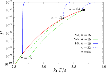
Figure 1: Phase diagram of semiflexible polymers in the pressure-temperature plane with chain length $N=32$ and for three values of the stiffness parameter, $\kappa$, as indicated. Vapor-isotropic (red), vapor-nematic (green), and isotropic-nematic (blue) branches are shown; the locations of the triple points for the three values of $\kappa$ are indicated with triangles; the vapor-isotropic branches terminate at the corresponding critical points, all three of which are very close to each other and are indicated by (nearly completely overlapping) black circles.

The advantage of the DFT approach to present a global view of the possible phase equilibria in the space of intensive thermodynamic variables emerges from this discussion clearly. However, it suffers to some extent from the neglect of statistical fluctuations, and this drawback is most prominent with respect to the description of the vapor-isotropic critical point; but as will be shown later in Sec. III.3, this aspect of the phase behavior can be studied reliably by MD.

III Simulation Results

III.1 The case of flexible polymers

We first focus on calculating the phase behavior of flexible polymers ($\kappa=0$). Note that, instead of varying the thermodynamic temperature of the system, $T$, we tuned the attractive part of the monomer-monomer interaction (see Eq. (1)) through $\lambda$, which changes the effective temperature of the system, $T_{\rm eff}$. A more extensive study of a similar model (including chain lengths from $N=8$ to $N=60$) has been recently presented by Silmore et al.Silmore, Howard, and Panagiotopoulos (2017), and our results are qualitatively consistent with that earlier work. In Fig. 2, a series of snapshots of the system is presented at different values of $T_{\rm eff}$. We observed coexistence of a low density vapor phase with a high density isotropic liquid phase. The density of the vapor phase increases, whereas the density of the isotropic liquid phase decreases as we approach the critical temperature, $T_{\rm c}$. At all effective temperatures $T_{\rm eff}<T_{\rm c}$ the formation of a liquid slab along the elongated $x$-axis is observed, which is expected because of the employed box geometry.

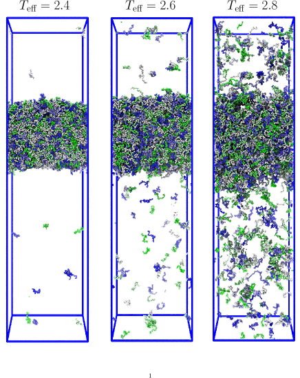
Figure 2: Snapshots of flexible polymers ($\kappa=0$) of length $N=16$ at different effective temperatures, $T_{\rm eff}$, as mentioned at the top of the figure.

In Fig. 3, we show the density distribution of monomers as a function of $x$ at different $T_{\rm eff}$. The two flat plateaus in the low and high density regions provide rough measures of the polymer-rich isotropic liquid density, $\rho_{{}_{\rm I}}$ and the polymer-diluted vapor density, $\rho_{{}_{\rm V}}$. When $T_{\rm eff}$ approaches the critical temperature, the difference between the two plateaus, i.e. $\Delta\rho=\rho_{{}_{\rm I}}-\rho_{{}_{\rm V}}$ (order-parameter for V-I transition), goes to zero, as expected. Note that for recording data such as shown in Fig. 3, one needs to superimpose the center of mass of the liquid regions at $x=\mathcal{L}_{x}/2=128\sigma$. We also emphasize that recording the apparent interfacial widths of the vapor-isotropic interface would be meaningful only when the dependence of these widths on the lateral box dimensions ($\mathcal{L}_{y}$ and $\mathcal{L}_{z}$) is analyzed, to account for the broadening due to capillary waves.Binder et al. (2001) This analysis has not been attempted here, however. More accurate estimates for $\rho_{{}_{\rm I}}$ and $\rho_{{}_{\rm V}}$ will be extracted from the finite size scaling analysis that will be presented below.

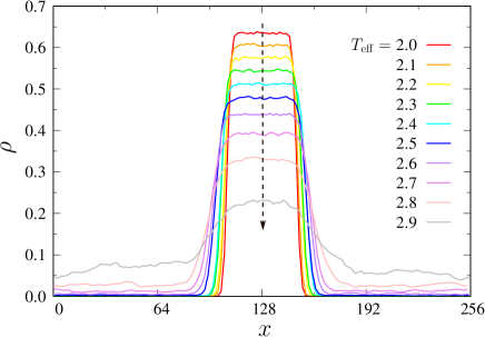
Figure 3: Monomer density profiles for flexible polymers ($\kappa=0$) of chain length $N=32$ as a function of $x$ at different values of $T_{\rm eff}$. The arrow indicates the vanishing density difference between the liquid and vapor phase as $T_{\rm eff}$ approaches the critical temperature, $T_{\rm c}$.

Performing our simulations at different values of $T_{\rm eff}$, we obtained the full phase diagram of flexible polymers for different chain lengths (Fig. 4(a)). Preliminary estimates for the critical temperature are calculated by fitting the order parameter, $\Delta\rho$, which is expected to be compatible with the universal scaling relation

$$\Delta\rho=B(1-T_{\rm eff}/T_{\rm c})^{\beta},$$ (10)

where $\beta$ is the critical exponent and $B$ is the material specific critical amplitude. For our fit, we took $\beta=0.325$, assuming that our model belongs to the $3d$-Ising model universality class as the interaction between the monomers is short-ranged. To estimate the critical density we consider the equation of rectilinear diameter

$$\rho_{{}_{\rm d}}=\frac{\rho_{{}_{\rm I}}+\rho_{{}_{\rm V}}}{2}=\rho_{\rm c}+C(T_{\rm c}-T_{\rm eff}),$$ (11)

where $C$ is a positive constant. We have observed an increase of $T_{\rm c}$ and a decrease of $\rho_{\rm c}$ with increasing chain length $N$, as expected. Qualitatively, a similar behavior was observed in our DFT calculations, as shown in Fig. 4(b). However, there are some notable quantitative differences between the DFT and the MD results due to the mean-field nature of the DFT calculations. For instance, the shape of the coexistence curve near the critical point is parabolic (i.e. $\beta=1/2$ in Eq. (10)). With the increase of chain length, the critical temperature $T_{\rm c}$ reaches an asymptotic value, whereas $\rho_{\rm c}$ decays to zero, typically, following a power-law $\rho_{\rm c}\sim 1/\sqrt{N}$ as predicted by Flory-Huggins theory.

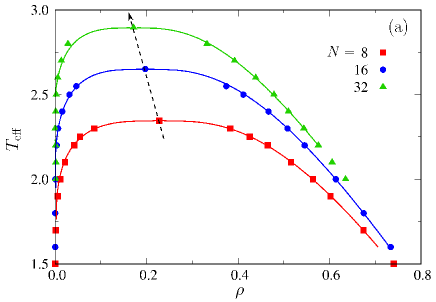
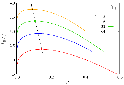
Figure 4: (a) Phase diagram of flexible polymers ($\kappa=0$) of lengths $N=8,16$ and $32$ from MD simulations. The arrow indicates the increase of the critical temperature $T_{\rm c}$ with increasing chain length, $N$. The critical density, $\rho_{\rm c}$, decreases with increasing $N$. Solid lines are the theoretical curves, obtained by fitting the simulation data to Eq. (10). (b) Phase digram from DFT calculations for chain lengths $N=8,16,32$ and $64$.

Flory-Huggins theoryFlory (1942); Huggins (1942); Flory (1953) predicts that for $N\to\infty$ the critical temperature $T_{\rm c}(N)$ approaches the $\Theta$-temperature, $T_{\Theta}$, as $T_{\Theta}-T_{\rm c}(N)\propto N^{-1/2}$. At the same time, the critical amplitude $B$ of the order parameter (see Eq. (10)) should also exhibit a singular $N$-dependence, $B(N)\propto N^{-1/4}$. However, previous simulations of lattice modelsWilding, Müller, and Binder (1996) as well as analyses of experimental dataEnders and Wolf (1995) have revealed that very long chains, orders of magnitude larger than available here and in related MD work,Silmore, Howard, and Panagiotopoulos (2017) are needed to allow a meaningful test of this singular $N$-dependence. Thus, there exists literature where even a slower decay of $\rho_{\rm c}$ is observed with the increase of chain length $N$: experiments are often fitted to $\rho_{\rm c}\propto N^{-0.38}$,Enders and Wolf (1995) and for the small $N$ investigated in Ref. 54 the decay exponent is even smaller, indicating that the asymptotic region of the power-law has not yet been reached.

III.2 Interplay of phase separation and nematic ordering for semiflexible polymers

After understanding the phase behavior of flexible polymers, now we pay attention to the phase behavior of semiflexible polymers ($\kappa>0$). In Fig. 5, we show snapshots of semiflexible polymers with chain length $N=32$ and stiffness constant $\kappa=16$ at different values of $T_{\rm eff}$. At temperature $T_{\rm eff}=2.9$ we observed coexistence of a nematic liquid with a polymer-diluted vapor phase. As we increase $T_{\rm eff}$, gradually a transition from nematic to isotropic occurs in the polymer-rich regions. There again we observed coexistence of an isotropic liquid with a vapor phase, as depicted in Fig. 5(b). We have shown the coexistence of a nematic liquid with an isotropic liquid in Fig. 5(c), which is obtained by fixing the overall density of the system close to the transition density.

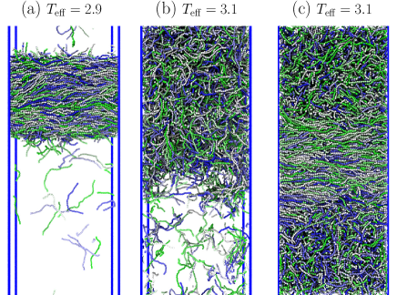
Figure 5: Snapshots of semiflexible polymers of length $N=32$ and stiffness $\kappa=16$ at three different temperatures, (a) $T_{\rm eff}=2.9$, where we observe coexistence of a nematic liquid with a vapor phase, (b) $T_{\rm eff}=3.1$, which is close to the critical temperature, where we observe the coexistence of an isotropic liquid with its vapor phase, and (c) $T_{\rm eff}=3.1$, where the coexistence of an isotropic liquid with a nematic liquid is shown (representing the “chimney” of the phase diagram, see Fig. 6 below).

The phase diagrams of semiflexible polymers with the same stiffness constant $\kappa=16$ but different chain lengths $N$ are presented in Fig. 6(a). In these phase diagrams, we have shown more clearly the V-N transition at low temperature, whereas, the V-I transition is observed at high temperature close to $T_{\rm c}$. The red arrows indicate roughly the I-N transition in the phase diagram. This transition can be quantified through the orientational order parameter, $S$, which is indicated by the color coding in the side bar. The orientational order parameter $S$ is the largest eigenvalue of the tensor $\mathscr{O}^{\alpha\beta}$, which we compute from averaging the tensor

$$\mathscr{O}^{\alpha\beta}_{ni}=\frac{1}{2}(3\textbf{u}^{\alpha}_{ni}\textbf{u}^{\beta}_{ni}-\delta_{\alpha\beta}),$$ (12)

over all bonds in the system (here $\alpha$ and $\beta$ stand for the Cartesian components, and $\mathbf{u}_{ni}$ is the unit vector from monomer $i$ towards monomer $i+1$ of the $n$-th chain). At low temperature, the red symbols (higher $S$ value) indicate the existence of an ordered nematic phase, whereas at high temperature the blue symbols indicate lower values of $S$ which are expected for the disordered isotropic phase. Note that near the triple point the I-N coexistence region is rather wide but becomes much narrower as $T_{\rm eff}$ increases (we denote this feature as a “chimney”-type phase diagram). For $N=32$ the chimney in the phase diagram is computed by fixing the overall monomer density in the system close to the value where the transition from nematic to isotropic liquid occurs.

From the data shown in Fig. 6(a) we also see that the critical temperature $T_{\rm c}$ increases with increasing chain length, $N$, whereas, the critical density, $\rho_{\rm c}$, decreases with increasing $N$. This behavior is quite similar to the case of flexible polymer with varying chain lengths. From our DFT calculation we also get similar results, which are presented in Fig. 6(b).

In Fig. 6(c), we have presented the phase diagram of semiflexible polymers with fixed chain length $N=32$ but different values of stiffness constant, i.e. $\kappa=0$, $8$ and $16$. For the flexible case ($\kappa=0$) we observed solely the V-I transition, whereas the semiflexible chains exhibited an additional V-N and I-N transition. At fixed chain length, the width of the nematic-isotropic transition increases with increasing chain stiffness. The critical temperature, $T_{\rm c}$, increases with increasing $\kappa$, because the effective mean-square radius of the chains increases with increasing bending rigidity. The DFT results also predict a similar behavior, as shown in Fig. 6(d). In Table 1 we have summarized the values of the critical temperature, $T_{\rm c}$, and critical density, $\rho_{\rm c}$, computed from DFT and extracted from our MD simulations by fitting the data to Eq. (10).

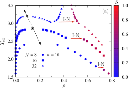
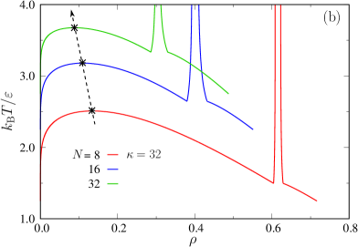
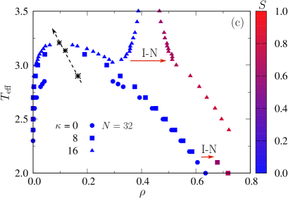
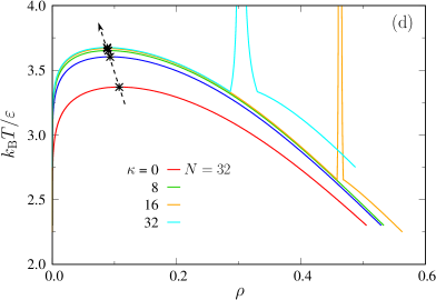
Figure 6: Phase diagram of semiflexible polymers: (a) Different chain length $N=8$, $16$ and $32$ and at fixed value of stiffness constant $k=16$. (b) Same as (a), but from DFT and at $\kappa=32$. (c) For fixed chain length $N=32$ and different values of the stiffness constant $\kappa=0$, $8$ and $16$. (d) Same as (c), but from DFT calculation. In (a) and (c), the red arrows are indicating the I-N transitions.

$\kappa$	$N$	$T_{\rm c}$ (DFT)	$\rho_{\rm c}$ (DFT)	$T_{\rm c}$ (MD)	$\rho_{\rm c}$ (MD)
0	8	2.375	0.145	2.346(2)	0.228(1)
0	16	2.930	0.127	2.651(3)	0.197(2)
0	32	3.370	0.108	2.895(2)	0.171(2)
8	8	2.501	0.135	2.427(3)	0.208(1)
8	16	3.109	0.111	2.813(3)	0.163(1)
8	32	3.651	0.089	3.135(2)	0.119(2)
16	8	2.508	0.135	2.452(3)	0.204(1)
16	16	3.120	0.110	2.864(5)	0.142(1)
16	32	3.675	0.088	3.205(5)	0.097(1)

Table 1: Values of the critical temperature, $T_{\rm c}$, and critical density, $\rho_{\rm c}$, for semiflexible chains with stiffness $\kappa$ and length $N$ from DFT and MD simulations. The results shown for the MD simulations have been computed by fitting the data to Eq. (10) with exponent $\beta=0.325$. Numbers is parentheses denote uncertainty in the last significant digit. For systems with $\kappa=16$, $N=16$ and with $\kappa=16$, $N=32$ we performed a finite size analysis (see Sec. III.3 below), and found $T_{\rm c}=2.865\pm 0.005$ and $T_{\rm c}=3.205\pm 0.005$, respectively.

The DFT calculations have the advantage that also the approach to the limiting behavior of stiff rods is easily investigated. For an example, Fig. 7(a) and (b) show the phase diagrams for the cases $\kappa=64$ and $\kappa=128$, respectively. While for $\kappa=64$ the triple temperature still is slightly lower than the vapor-isotropic critical point, for $\kappa=128$ no triple point exists any longer; the triple point and the critical point have merged at some intermediate value of $\kappa$, and for $\kappa=128$ phase equilibria between vapor and isotropic liquid are no longer stable. When we follow the nematic order parameter along the coexistence curve of the nematically ordered phase with the corresponding dense fluid (for temperatures lower than the triple temperature) and further at high temperatures (when the isotropic phase is more dilute) a clear kink at the triple temperature is observed (Fig. 7(c)). As $\kappa$ increases, the discontinuity in slope becomes smaller and vanishes when the critical and triple temperature merge.

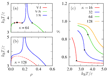
Figure 7: (a) Phase diagram of semiflexible polymers in the density-temperature plane with chain length $N=32$ and stiffness constant $\kappa=64$. The V-I critical point is shown by the circle and the V-I-N triple point is indicated by three triangles. (b) Same as (a) but for $\kappa=128$. The red dashed curve corresponds to the metastable V-I equilibrium. (c) Order parameter $S$ as a function of temperature along V-N and I-N coexistence curves for a semiflexible chain of length $N=32$ and four values of the stiffness parameter, $\kappa=16$, $32$, $64$ and $128$. The discontinuity in the slope for the three lower values of $\kappa$ corresponds to the triple point.

In principle, the order parameter $S$ at isotropic-nematic coexistence is accessible also by MD simulation, when we record $S$ as a function of the effective temperature $T_{\rm eff}$ (see Fig. 8(a)) at fixed $N$ and fixed $\kappa$. The MD approach has the additional advantage that also chain linear dimensions are readily accessible in both phases, as shown in Figs. 8(b).

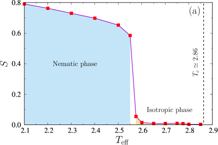
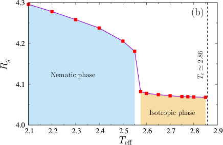
Figure 8: (a) Orientational order parameter, $S$, vs. effective temperature, $T_{\rm eff}$, for $N=16$ and $\kappa=16$, (b) radius of gyration, $R_{\rm g}$, vs. $T_{\rm eff}$. The nematic order parameter $S$ has been calculated only for the polymer rich regions (not for the whole system), whereas $R_{\rm g}$ is computed for the entire simulation box.

III.3 Finite size scaling analysis of the vapor-isotropic transition of semiflexible polymers

In the previous sections, the critical point was determined by fitting Eqs. (10) and (11) to the simulation data. However, values obtained through this procedure are not always reliable because of finite-size effects. During this fitting one should be careful when selecting the range of simulation data, which should not be affected by the system size. Otherwise, we may arrive at an inaccurate estimation of the critical point. In order to control these finite size effects, we shall apply here finite size scaling analyses of subbox density distributions (some background on this technique is discussed in the Appendix). The advantage of the finite size scaling method is that it allows to both estimate the critical point from the crossings of the fourth order cumulants of the order parameter, and to estimate the critical exponents $\nu$ and $\beta$ (whereas in Eq. (10), $\beta$ needs to be assumed). The fourth order cumulant is defined in terms of the order parameter $m$ in a subbox of linear dimension $l$ as

$$Q_{l}=\frac{\left\langle m^{4}\right\rangle_{l}}{\left\langle m^{2}\right\rangle^{2}_{l}}$$ (13)

where $\left\langle m^{2}\right\rangle_{l}$ and $\left\langle m^{4}\right\rangle_{l}$ are the second and fourth moment of the order parameter, respectively, defined as

$$\left\langle m^{2}\right\rangle_{l}=\frac{1}{2}\left[\sum_{i}(\rho_{{}_{{\rm I},i}}-\rho_{{}_{\rm d}})^{2}+\sum_{i}(\rho_{{}_{{\rm V},i}}-\rho_{{}_{\rm d}})^{2}\right],$$

$$\left\langle m^{4}\right\rangle_{l}=\frac{1}{2}\left[\sum_{i}(\rho_{{}_{{\rm I},i}}-\rho_{{}_{\rm d}})^{4}+\sum_{i}(\rho_{{}_{{\rm V},i}}-\rho_{{}_{\rm d}})^{4}\right]$$ (14)

where $\rho_{{}_{\rm d}}=(\rho_{{}_{\rm I}}+\rho_{{}_{\rm V}})/2$ is the coexistence diameter, and the averages are carried out over cubic $l\times l\times l$ subboxes of the total system. Half of the subboxes that are averaged over are placed in the region of the liquid-like phase and half in the vapor-like phase (see the Appendix for details). Note that for an Ising magnet, the distribution of the order parameter $m$ (the magnetization) is strictly symmetric between the coexisting phases having opposite sign; no such spin reversal-type symmetry exists between the coexisting liquid and vapor phases of fluid systems, however. Thus, we take $\rho_{{}_{\rm I}}-\rho_{{}_{\rm d}}$ and $\rho_{{}_{\rm V}}-\rho_{{}_{\rm d}}$ as the analogs of the phases with positive and negative magnetization, and average their moments (see Eq. (14)).

Instead of calculating the cumulant by dividing the whole simulation box into subboxes, we placed subboxes only inside the pure phases to avoid the presence of interfaces, as discussed in more detail in the Appendix. As seen in Fig. 9, we vary the subbox linear dimension $l$ from $l=16\,\sigma$ to $l=28\,\sigma$, so the subboxes always contain a large number of monomers. A reasonably accurate intersection point for the case $\kappa=16$, $N=32$ is found at $T_{\rm c}\approx 3.205\pm 0.005$, and for the case $\kappa=16$, $N=16$ at $T_{\rm c}\approx 2.865\pm 0.005$. Due to both statistical errors and systematic errors because of corrections to finite size scaling (which holds strictly only in the asymptotic limit $l\to\infty$), the error of about $\pm 0.005$ cannot be easily reduced. Nonetheless, we consider the obtained accuracy as rather satisfactory. The estimates obtained from Fig. 9(a) and (b) are in excellent agreement with the estimates from the fits using Eq. (10); hence we did not extend the large effort of the finite scaling analysis to other combinations of $\kappa$ and $N$.

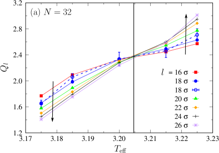
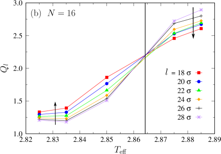
Figure 9: (a) Cumulant $Q_{l}=\left\langle m^{4}\right\rangle_{l}/\left\langle m^{2}\right\rangle^{2}_{l}$ vs. $T_{\rm eff}$ for different subbox sizes, $l$, as indicated, at $\kappa=16$ and $N=32$. Open circles with error bars represent results obtained from a different system size, where we maintain the aspect ratio $l/\mathcal{L}_{y}=l/\mathcal{L}_{z}=1/2$ (see Appendix). (b) Same plot as (a), but at $\kappa=16$ and $N=16$. In both panels, the solid vertical lines correspond to the location of the estimated critical temperature, $T_{\rm c}$.

The cumulant, $Q_{l}$, and the second moment, $\left\langle m^{2}\right\rangle$, pursue certain universal relations, some of them are quoted below for $T_{\rm eff}=T_{\rm c}$,

$$\delta Q_{l}/\delta T_{\rm eff}\propto l^{1/\nu};~{}~{}~{}~{}~{}l^{3}\left\langle m^{2}\right\rangle\propto l^{(3-2\beta/\nu)}$$ (15)

For $T_{\rm eff}<T_{\rm c}$ and large enough $\ell$, $\sqrt{\left\langle m^{2}\right\rangle}$ approaches the behavior of the order parameter, $\sqrt{\left\langle m^{2}\right\rangle}\propto|T_{\rm c}-T_{\rm eff}|^{\beta}$. These scaling relations are tested in our simulations to check the compatibility of the critical exponents with the $3d$-Ising universality class. In Fig. 10(a) and (b), we have presented the plot of $\sqrt{\left\langle m^{2}\right\rangle}$ as a function of $T_{\rm c}-T_{\rm eff}$. In both cases, consistency of our simulation data with the theoretical solid lines recovers the critical exponent $\beta\approx 0.325$, which was assumed in our previous fitting exercises. In Fig. 11(a) and (b), we show the plots of $\delta Q_{l}/\delta T_{\rm eff}$ and $l^{3}\left\langle m^{2}\right\rangle$, respectively, as a function of $l$. In both cases, our simulation data exhibit power-law behavior and show consistency with the existing theoretical predictions. While the accuracy with which the exponent $3-2\beta/\nu$ can be estimated is rather satisfactory, only a rough estimate for $1/\nu$ is obtained. However, a better accuracy of $\nu$ is found when we consider the interfacial tension, $\gamma$, to which we turn next. Nevertheless, recovering the critical exponents $\beta$ and $\nu$, we confirm that our current model indeed belongs to the $3d$-Ising universality class, as hypothesized initially.

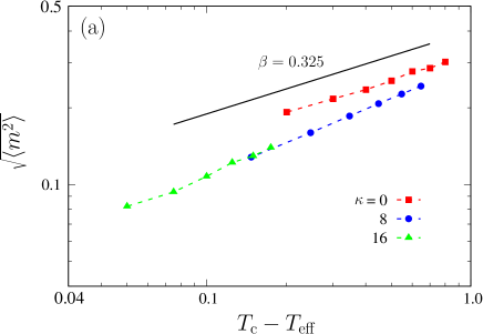
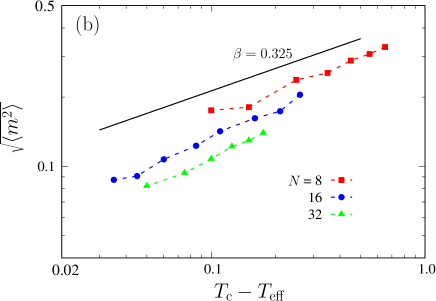
Figure 10: (a) Log-log plot of $\sqrt{\left\langle m^{2}\right\rangle}$ for the largest subbox ($l=28\sigma$) as a function of $T_{\rm c}-T_{\rm eff}$ for fixed chain length $N=32$ and different values for the stiffness constant $\kappa=0$, $8$, and $16$. (b) Same as (a), for fixed $\kappa=16$ and different chain lengths $N=8$, $16$ and $32$. The solid lines correspond to the theoretical power-law behavior.

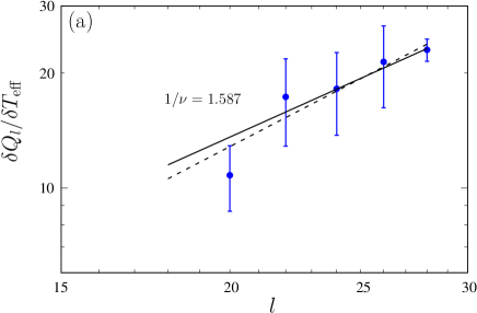
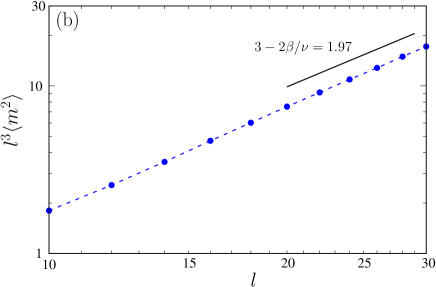
Figure 11: (a) $\delta Q_{l}/\delta T_{\rm eff}$ vs. subbox size, $l$, at $\kappa=16$ and $N=32$ on a log-log scale. The solid line is the theoretical expectation, $\delta Q_{l}/\delta T_{\rm eff}\propto l^{1/\nu}$ with $1/\nu=1.587$. The dashed line is a power-law fit to the simulation data, providing an exponent of $1/\nu=1.83\pm 0.35$. (b) $l^{3}\left\langle m^{2}\right\rangle_{l}$ vs. $l$ on a log-log scale, at critical temperature $T_{\rm c}=3.205$. The solid line corresponds to a power-law with an exponent of $1.97$.

Since the elongated geometry of our simulation box always implies the presence of two interfaces for temperatures $T_{\rm eff}<T_{\rm c}$ (see Fig. 3), one can use the well-known Kirkwood-Buff relation

$$\gamma=\frac{\mathcal{L}_{x}}{2}\left\langle P_{xx}-\frac{P_{yy}+P_{zz}}{2}\right\rangle$$ (16)

to estimate the interfacial tension $\gamma$ of the studied systems from the anisotropy of their pressure tensors. In Eq. (16), $P_{xx}$, $P_{yy}$, and $P_{zz}$ are the diagonal components of the pressure tensor along the $x$, $y$, and $z$ direction, respectively. Finally, in Fig. 12(a) and (b), we show the compatibility of our simulation data with the expected critical behavior, $\gamma=\gamma_{0}(1-T_{\rm eff}/T_{\rm c})^{2\nu}=\gamma_{0}(1-T_{\rm eff}/T_{\rm c})^{1.26}$. For fixed $\kappa$ and increasing $N$, one can recognize that the amplitude $\gamma_{0}$ strongly decreases. For flexible polymers, one expects that $\gamma_{0}$ exhibits a scaling relation due to Widom,Widom (1988) i.e. $\gamma_{0}(N)\propto N^{-(1-\nu)}\approx N^{-0.37}$, while in mean field theory a different power-law applies close to $T_{\rm c}$, namely $\gamma_{0}(N)\propto N^{-1/4}$. However, we are not aware of work exploring the effect of chain stiffness on $\gamma_{0}$. Again, we add the caveat that for $N\leq 32$ we presumably have not reached the region of large enough $N$ where the discussed power-laws would be applicable.

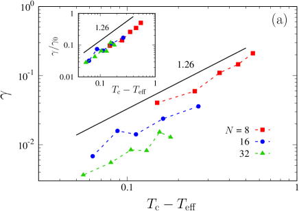
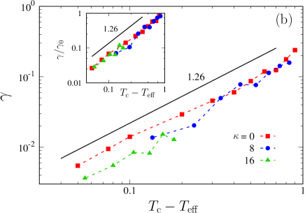
Figure 12: (a) Surface tension, $\gamma$, vs. $T_{\rm c}-T_{\rm eff}$ for three different chain lengths $N=8$, $16$, and $32$ with $\kappa=16$, on a log-log scale. The solid lines represent power-laws with an exponent $\mu\simeq 1.26$, which is the theoretical expectation for the $3d$-Ising universality class. The inset shows the plot of $\gamma/\gamma_{0}$ vs. $T_{\rm c}-T_{\rm eff}$ ($\gamma=\gamma_{0}(T_{\rm c}-T_{\rm eff})^{\mu}$, $\gamma_{0}$ being the amplitude of the surface tension). (b) Same plot as (a), for different values of $\kappa=0$, $8$, and $16$ at fixed chain length $N=32$.

IV Conclusions

In the present work, we have studied the phase behavior of flexible and semiflexible polymers in a lyotropic solution of varying quality via state-of-the-art MD simulations and DFT calculations. We focus on a coarse-grained bead-spring type model with a bond-angle for the polymers throughout, and the solvent molecules are not explicitly considered. The solvent quality is controlled by adjusting the strength of the attractive part of the effective interaction between the monomeric units. In contrast to the Maier-Saupe model, there is no explicit anisotropy in the interaction between monomeric units from different chains (although such an anisotropy might arise on coarse-grained scales due to the intrinsic stiffness of the polymer chains and entropic effects). As in the Maier-Saupe model, not only we can control the isotropic-nematic phase transition by varying the (effective) temperature, but also we can pay attention to the variation of the polymer concentration in the solution (or, correspondingly, the density of monomers in the considered volume). As a limiting special case, we treat phase separation of a solution of flexible polymers as well, and obtain qualitative agreement of the resulting phase diagrams with related earlier studies.Silmore, Howard, and Panagiotopoulos (2017)

For the solutions of semiflexible polymers, and relatively small stiffness, we find a phase diagram with a vapor-isotropic critical point at small monomer density, whereas, at large monomer densities a nematic-isotropic transition between a rather dense isotropic solution and the nematic phase is observed at a temperature above the triple point temperature. While right at and near the triple point temperature the nematic-isotropic two-phase coexistence region is rather wide and it narrows with the increase of temperature, thus, exhibiting a “chimney”-type topology in the phase diagram in the temperature-density plane. When the chain stiffness increases, the triple temperature increases strongly, whereas the critical temperature increases only a little bit. Thus, a stiffness is reached where the triple point temperature and the critical temperature become equal, and vapor-isotropic liquid coexistence disappears. Above this stiffness value only a single transition from isotropic fluid to nematic is observed at any temperature, with “swan neck”-topology (at low $T$, the isotropic fluid is gas-like, but gradually changes to dense liquid on the back of the swan). This changeover of the phase diagram topology is most easily described in the phase diagram using only intensive thermodynamic variables ($T$, $P$), cf. Fig. 1.

While DFT and MD results agree qualitatively (see Fig. 6), quantitative details differ; part of the difference originates from the (necessary) use of slightly different models, partly due to approximate statistical mechanics implied by the DFT treatment. For example, DFT does not yield the Ising-model character of the critical behavior associated with the vapor-isotropic type critical point, which is verified by our MD calculations. For the latter purpose, use of a subsystem finite size scaling method avoiding subboxes containing interfacial contributions has been applied here, and found to be useful.

An intriguing problem that we have not addressed here is the limiting behavior of various quantities (in particular $T_{\rm c}(N)$, $\rho_{\rm c}(N)$, critical amplitudes) as the chain length $N$ tends to infinity; this issue still is far beyond the computational resources available to us. Another aspect that will be interesting for future work is the structure of interfaces between the nematic phase and coexisting isotropic phases with high or low monomer density, respectively. We also remark that at high monomer densities further phases appear, such as smectic and crystalline phases, but such phenomena also must be left for future work.

While our models lack any chemical specificity, and hence a direct comparison with experimental data would be premature, we hope that our model calculations will stimulate more experimental work exploring the effect of solvent quality on the behavior of solutions containing semiflexible polymers.

Appendix A Finite size scaling of vapor-isotropic transitions in the canonical ensemble

Our estimation of critical properties in terms of Eqs. (10) and (11) suffers from some uncertainties: (i) Eq. (10) is believed to hold in the limit $T-T_{\rm c}\to 0$ in the thermodynamic limit (number of particles $\mathcal{N}\to\infty$). A priori it is not clear how small $1-T/T_{\rm c}$ has to be such that Eq. (10) is accurate. A small error in the fitted value of $T_{\rm c}$ could be compensated by an error in the fitted value of the amplitude $B$. (ii) The estimates for $\Delta\rho=\rho_{{}_{\rm I}}-\rho_{{}_{\rm V}}$ that are fitted may suffer from small but systematic finite size effects. (iii) The linear dependence of $\rho_{\rm d}$ on $T$ [Eq. (11)] holds only approximately. At temperatures close to $T_{\rm c}$ deviations must occur.Kim, Fisher, and Luijten (2003); Kim and Fisher (2003) Thus, it has been widely accepted that a more reliable estimation of critical properties by computer simulation should be based on a finite size scaling analysis.Landau and Binder (2015) In the context of Monte Carlo simulations, this approach is conveniently implemented in the grand-canonical $\mu VT$ ensemble, with $\mu$ being the chemical potential of the particles. For $T$ close enough to $T_{\rm c}$ and large enough linear dimensions $l$ of the system, the probability distribution of the density at $\mu=\mu_{\rm coex}(T)$, the value where coexistence between vapor and liquid occurs for $V\to\infty$, is

$$p(\rho)=l^{\beta/\nu}\tilde{p}\left\{\left(\rho-\rho_{\rm c}\right)l^{\beta/\nu},l^{1/\nu}\tau\right\}$$ (17)

where $\beta$ and $\nu$ are the critical exponents of order parameter and correlation length, $\tau=1-T/T_{\rm c}$, and $\tilde{p}$ is a scaling function. Equation (17) holds asymptotically in the limit where $\tau\to 0$, $l\to\infty$, but $l^{1/\nu}\tau$ can still vary. From Eq. (17), readily moments of this distribution can be expressed as

$$\left\langle m^{2k}\right\rangle_{l}=l^{-2k\beta/\nu}f_{2k}(l^{1/\nu}\tau),$$ (18)

with $m=\rho_{{}_{\rm I}}-\rho_{{}_{\rm V}}$ and $f_{2k}$ being another scaling function, whose explicit form we shall not need. Particularly useful is the ratio

$$Q_{l}=\left\langle m^{2}\right\rangle^{2}_{l}/\left\langle m^{4}\right\rangle_{l}=\tilde{Q}(l^{1/\nu}\tau)$$ (19)

Since in this cumulant ratio the power-law prefactors have canceled, $Q_{l}$ depends on $l$ via the variable $l^{1/\nu}\tau$ only. Consequently, when we plot $Q_{l}$ vs. $\tau$ for several choices of $l$, we should find that all curves $Q_{l}(\tau)$ must intersect at a unique crossing point $\tilde{Q}(0)$. Thus, $T_{\rm c}$ can be found by locating this intersection, and there is no need to fit multiple parameters. The slope $({\rm d}Q_{l}/{\rm d}\tau)_{\tau=0}\propto l^{1/\nu}$ then yields information on the exponent $1/\nu$. Similarly, from $\left\langle(\Delta\rho)^{2}\right\rangle_{l,T=T_{\rm c}}\propto l^{-2\beta/\nu}$ we find the second exponent ratio $\beta/\nu$. This approach has found useful applications in numerous systems.Landau and Binder (2015)

However, in the context of MD simulations, the particle number is typically constant, and thus the $\mu VT$ ensemble cannot be used (and for systems containing long polymers, Monte Carlo simulations at constant $\mu$ would not be practical either, because the success rate for inserting long polymers in a dense fluid is vanishingly small).

In this dilemma, it has been advocatedRovere, Heermann, and Binder (1990); Rovere, Nielaba, and Binder (1993) to study subsystems of linear dimension $l$, such that $l\ll\mathcal{L}$. Indeed, when $\mathcal{L}\to\infty$, a subsystem (with virtual boundaries, allowing exchange of particles through its surfaces) would realize the grand-canonical ensemble of the total system. However, this approach seriously suffers from two problems: (i) since $\mathcal{L}$ is finite, the system is not strictly grand-canonical, and an additional variable $l/\mathcal{L}$ needs to be added to Eq. (17). Choosing subsystems of several sizes $l$, the variation due to this extra variable $l/\mathcal{L}$ to some extent spoils relations (18) and (19). (ii) When $\rho$ is chosen at $\rho_{\rm c}$ or nearby, for $T<T_{\rm c}$ some subboxes will not be dominated by contributions where $\rho$ is either close to $\rho_{{}_{\rm V}}$ or close to $\rho_{{}_{\rm I}}$ (which is desirable), but will be influenced by contributions from one of the two interfaces between the coexisting phases necessarily present in the system. This gives rise to further systematic errors.

Both problems can be avoided by a recent extension of the method,Siebert et al. (2018) where one chooses an elongated geometry $\mathcal{L}_{x}\times\mathcal{L}\times\mathcal{L}$ with, e.g., $\mathcal{L}_{x}=3L$, which ensures that the two interfaces in the system, when present, are oriented perpendicular to the $x$-axis, and one puts subboxes of the linear dimension $l=\mathcal{L}/2$ in the liquid domain as well as in the vapor domain only, so none of the subboxes are affected by interfacial contributions. In that case, there hence would be $4$ liquid $l\times l\times l$ subboxes either side (recalling the periodic boundary conditions). In order to achieve such a setup, one computes in each configuration for which the subsystem distributions shall be recorded the center of mass position of the system, and requests that its $x$-coordinate coincides with the center of mass coordinate of the liquid boxes.

This arrangement does not strictly realize the grand-canonical ensemble, but there occurs still enough exchange of chains in the boxes with chains in the intermediate regions where the interfaces are. The resulting distribution function $p(\rho)$ of these subboxes hence still has the same scaling structure as written in Eq. (17) for the grand-canonical ensemble, so the precise form of the scaling function $\tilde{p}$ is somewhat different. We also note that in such a setup the second variable $l/\mathcal{L}=1/2$ still is present, but since we keep it strictly constant when we study a range of choices for $l$ (or $\mathcal{L}$, respectively), this does not disturb our analysis. We note that Siebert et al.Siebert et al. (2018) validated the approach for the $2d$-Ising model, where both $T_{\rm c}$ and the critical exponents are exactly known. The disadvantage of this approachSiebert et al. (2018) is the need of precise simulation data for a range of large systems, when $l$ is varied over an extended range. Therefore, we followed in the present application the approximation of Refs. 77 and 78 to use only subsystems with varying $l$ for one very large system, but follow Siebert et al.Siebert et al. (2018) choosing an elongated geometry with subboxes avoiding the interfacial regions. We tested one smaller system ($\mathcal{L}_{x}=144\sigma$, $\mathcal{L}_{y}=\mathcal{L}_{z}=36\sigma$) to compute subsystem moments for $l=18\sigma$, and found that within our statistical uncertainty the moments $\left\langle m^{2}\right\rangle_{l}$ and $\left\langle m^{4}\right\rangle_{l}$ were the same as in the larger systems. Hence, our approximation did not cause significant errors.

References

- Ciferri, Krigbaum, and Meyer (1982) A. Ciferri, W. R. Krigbaum, and R. B. Meyer, eds., Polymer Liquid Crystals (Academic, New York, 1982).
- Ciferri (1983) A. Ciferri, ed., Liquid Crystallinity in Polymers: Principles and Fundamental Properties (VCH Publishers, New York, 1983).
- Donald, Windle, and Hanna (2006) A. M. Donald, A. H. Windle, and S. Hanna, Liquid crystalline polymers (Cambridge University Press, Cambridge, 2006).
- Brown and Wolsen (1979) G. H. Brown and J. J. Wolsen, Liquid Crystals and Biological Structures (Academic Press, New York, 1979).
- Köster et al. (2015) S. Köster, D. A. Weitz, R. D. Goldman, U. Aebi, and H. Herrmann, Curr. Opin. Cell Biol. 32, 82 (2015).
- Grosberg and Khokhlov (1981) A. Y. Grosberg and A. R. Khokhlov, Adv. Polym. Sci. 41, 53 (1981).
- Khokhlov and Semenov (1981) A. R. Khokhlov and A. N. Semenov, Physica A 108, 546 (1981).
- Khokhlov and Semenov (1982a) A. R. Khokhlov and A. N. Semenov, Physica A 112, 605 (1982a).
- Khokhlov and Semenov (1982b) A. R. Khokhlov and A. N. Semenov, J. Phys. A: Math. Gen. 15, L361 (1982b).
- Odijk (1983) T. Odijk, Macromolecules 16, 1340 (1983).
- Khokhlov and Semenov (1985) A. R. Khokhlov and A. N. Semenov, J. Stat. Phys. 38, 161 (1985).
- Odijk (1985) T. Odijk, Polym. Commun. 26, 197 (1985).
- Odijk (1986a) T. Odijk, Macromolecules 19, 2313 (1986a).
- Odijk (1986b) T. Odijk, Liq. Cryst. 1, 553 (1986b).
- Grosberg and Zhestkov (1986) A. Y. Grosberg and A. V. Zhestkov, Polym. Sci. U.S.S.R. 28, 97 (1986).
- Vroege and Odijk (1988) G. J. Vroege and T. Odijk, Macromolecules 21, 2848 (1988).
- Shimada, Doi, and Okano (1988) T. Shimada, M. Doi, and K. Okano, J. Phys. Soc. Jpn. 57, 2432 (1988).
- Hentschke (1990) R. Hentschke, Macromolecules 23, 1192 (1990).
- Taylor and Herzfeld (1990) M. P. Taylor and J. Herzfeld, Langmuir 6, 911 (1990).
- Hentschke and Herzfeld (1991) R. Hentschke and J. Herzfeld, Phys. Rev. A 44, 1148 (1991).
- DuPré and Yang (1991) D. B. DuPré and S.-J. Yang, J. Chem. Phys. 94, 7466 (1991).
- Selinger and Bruinsma (1991a) J. V. Selinger and R. F. Bruinsma, Phys. Rev. A 43, 2910 (1991a).
- Selinger and Bruinsma (1991b) J. V. Selinger and R. F. Bruinsma, Phys. Rev. A 43, 2922 (1991b).
- Chen (1993) Z.-Y. Chen, Macromolecules 26, 3419 (1993).
- Sato and Teramoto (1994) T. Sato and A. Teramoto, Acta Polym. 49, 399 (1994).
- Sato and Teramoto (1996a) T. Sato and A. Teramoto, Adv. Polym. Sci. 126, 85 (1996a).
- Sato and Teramoto (1996b) T. Sato and A. Teramoto, Macromolecules 29, 4107 (1996b).
- Egorov, Milchev, and Binder (2016) S. A. Egorov, A. Milchev, and K. Binder, Phys. Rev. Lett. 116, 187801 (2016).
- Egorov et al. (2016) S. A. Egorov, A. Milchev, P. Virnau, and K. Binder, Soft Matter 12, 4944 (2016).
- Milchev et al. (2018) A. Milchev, S. A. Egorov, K. Binder, and A. Nikoubashman, J. Chem. Phys. 149, 174909 (2018).
- Onsager (1949) L. Onsager, Ann. N. Y. Acad. Sci. 51, 627 (1949).
- Fraden (1995) S. Fraden, “Observation, prediction and simulation of phase transitions in complex fluids,” (Kluwer Academic Publishers, Dordrecht, 1995) p. 113.
- Lekkerkerker and Tuinier (2011) H. N. W. Lekkerkerker and R. Tuinier, Colloids and the Depletion Interaction (Springer, Dordrecht, 2011).
- Wilson and Allen (1993) M. R. Wilson and M. P. Allen, Mol. Phys. 80, 277 (1993).
- Dijkstra and Frenkel (1995) M. Dijkstra and D. Frenkel, Phys. Rev. E 51, 5891 (1995).
- Kamien and Grest (1997) R. D. Kamien and G. S. Grest, Phys. Rev. E 55, 1197 (1997).
- Lyulin et al. (1998) A. V. Lyulin, M. S. Al-Barwani, M. P. Allen, M. R. Wilson, I. Neelov, and N. K. Allsopp, Macromolecules 31, 4626 (1998).
- Naderi and van der Schoot (2014) S. Naderi and P. van der Schoot, J. Chem. Phys. 141, 124901 (2014).
- de Braaf et al. (2017) B. de Braaf, M. O. Menegon, S. Paquay, and P. van der Schoot, J. Chem. Phys. 147, 244901 (2017).
- Yamakawa (1971) H. Yamakawa, Modern theory of polymer solutions (Harper and Row, New York, 1971).
- de Gennes (1979) P. G. de Gennes, Scaling Concepts in Polymer Physics (Cornell University Press, Ithaca, NY, 1979).
- Grosberg and Khokhlov (1994) A. Y. Grosberg and A. R. Khokhlov, Statistical Physics of Macromolecules (AIP Press, Woodbury, 1994).
- Rubinstein and Colby (2003) M. Rubinstein and R. H. Colby, Polymer physics (Oxford University Press, Oxford, 2003).
- Hsu, Paul, and Binder (2010) H.-P. Hsu, W. Paul, and K. Binder, Macromolecules 43, 3094 (2010).
- van der Schoot and Odijk (1992) P. van der Schoot and T. Odijk, J. Chem. Phys. 97, 515 (1992).
- Lekkerkerker and Stroobants (1994) H. N. W. Lekkerkerker and A. Stroobants, Nuovo Cimento D 16, 949 (1994).
- Bolhuis and Frenkel (1997) P. Bolhuis and D. Frenkel, J. Chem. Phys. 106, 666 (1997).
- Jungblut et al. (2007) S. Jungblut, R. Tuinier, K. Binder, and T. Schilling, J. Chem. Phys. 127, 244909 (2007).
- Cotter (1977) M. A. Cotter, J. Chem. Phys. 66, 1098 (1977).
- Stanley (1971) H. E. Stanley, Introduction to Phase Transitions and Critical Phenomena (Oxford University Press, Oxford, 1971).
- Milchev, Nikoubashman, and Binder (2019) A. Milchev, A. Nikoubashman, and K. Binder, Comput. Mater. Sci. 166, 230 (2019).
- Allen and Tildesley (2017) M. P. Allen and D. J. Tildesley, Computer Simulation of Liquids, 2nd ed. (Oxford University Press, Oxford, 2017).
- Wilding, Müller, and Binder (1996) N. B. Wilding, M. Müller, and K. Binder, J. Chem. Phys. 105, 802 (1996).
- Silmore, Howard, and Panagiotopoulos (2017) K. S. Silmore, M. P. Howard, and A. Z. Panagiotopoulos, Mol. Phys. 115, 320 (2017).
- de Gennes and Prost (1995) P. G. de Gennes and J. Prost, The Physics of Liquid Crystals, 2nd ed. (Clarendon Press, Oxford, 1995).
- Daoulas, Rühle, and Kremer (2012) K. C. Daoulas, V. Rühle, and K. Kremer, J. Phys. Condens. Matter 24, 284121 (2012).
- Gemünden and Daoulas (2015) P. Gemünden and K. C. Daoulas, Soft Matter 11, 532 (2015).
- Siebert et al. (2018) J. T. Siebert, F. Dittrich, F. Schmid, K. Binder, T. Speck, and P. Virnau, Phys. Rev. E 98, 030601(R) (2018).
- Grest and Kremer (1986) G. S. Grest and K. Kremer, Phys. Rev. A 33, 3628 (1986).
- Anderson, Lorenz, and Travesset (2008) J. A. Anderson, C. D. Lorenz, and A. Travesset, J. Comput. Phys. 227, 5342 (2008).
- Glaser et al. (2015) J. Glaser, T. D. Nguyen, J. A. Anderson, P. Lui, F. Spiga, J. A. Millan, D. C. Morse, and S. C. Glotzer, Comput. Phys. Commun. 192, 97 (2015).
- Johnson, Zollweg, and Gubbins (1993) J. K. Johnson, J. A. Zollweg, and K. E. Gubbins, Mol. Phys. 78, 591 (1993).
- Müller, MacDowell, and Yethiraj (2003) M. Müller, L. G. MacDowell, and A. Yethiraj, J. Chem. Phys. 118, 2929 (2003).
- Egorov (2004) S. A. Egorov, Phys. Rev. E 70, 031402 (2004).
- Egorov (2005) S. A. Egorov, Phys. Rev. E 72, 010401(R) (2005).
- Patel and Egorov (2005) N. Patel and S. A. Egorov, J. Chem. Phys. 123, 144916 (2005).
- Egorov (2008) S. A. Egorov, J. Chem. Phys. 129, 064901 (2008).
- Binder et al. (2001) K. Binder, M. Müller, F. Schmid, and A. Werner, Adv. Colloid Interface Sci. 94, 237 (2001).
- Flory (1942) P. J. Flory, J. Chem. Phys. 10, 51 (1942).
- Huggins (1942) M. L. Huggins, J. Phys. Chem. 46, 151 (1942).
- Flory (1953) P. J. Flory, Principles of Polymer Chemistry (Cornell University Press, Ithaca, NY, 1953).
- Enders and Wolf (1995) S. Enders and B. A. Wolf, J. Chem. Phys. 103, 3809 (1995).
- Widom (1988) B. Widom, J. Stat. Phys. 52, 1343 (1988).
- Kim, Fisher, and Luijten (2003) Y. C. Kim, M. E. Fisher, and E. Luijten, Phys. Rev. Lett. 91, 065701 (2003).
- Kim and Fisher (2003) Y. C. Kim and M. E. Fisher, Phys. Rev. E 68, 041506 (2003).
- Landau and Binder (2015) D. P. Landau and K. Binder, A guide to Monte Carlo simulations in statistical physics, 4th ed. (Cambridge University Press, Cambridge, 2015).
- Rovere, Heermann, and Binder (1990) M. Rovere, D. W. Heermann, and K. Binder, J. Phys. Condens. Matter 2, 7009 (1990).
- Rovere, Nielaba, and Binder (1993) M. Rovere, P. Nielaba, and K. Binder, Z. Physik B - Condensed Matter 90, 215 (1993).