Osculating Versus Intersecting Circles in Space-Based Microlens Parallax Degeneracies

1 Introduction

In his original paper on space-based microlens parallax measurements, Refsdal (1966) already noted that they were subject to a discrete four-fold degeneracy. Two observatories, one on Earth and one on a satellite, would each see a single-lens single-source (1L1S) microlensing event, characterized by three Paczyński (1986) parameters $(t_{0},u_{0},t_{\rm E})$, but these parameters would differ due to their different viewpoints. Here $t_{0}$ is the time of maximum magnification, $u_{0}$ is the impact parameter normalized to the Einstein radius $\theta_{\rm E}$, and $t_{\rm E}$ is the Einstein timescale,

$$t_{\rm E}\equiv{\theta_{\rm E}\over\mu_{\rm geo}};\quad\theta_{\rm E}^{2}=\kappa M\pi_{\rm rel},$$ (1)

where $M$ is the mass of the lens, $(\pi_{\rm rel},{\mbox{\boldmath$\mu$}}_{\rm geo})$ are the lens-source relative (parallax, proper motion) and $\kappa\equiv 4G/c^{2}{\rm AU}\simeq 8.14\,{\rm mas}\,M_{\odot}^{-1}$. In more modern language (Gould, 2000, 2004; Gould & Horne, 2013), the microlens parallax vector,

$${\mbox{\boldmath$\pi$}}_{\rm E}\equiv{\pi_{\rm rel}\over\theta_{\rm E}}\,{{\mbox{\boldmath$\mu$}}_{\rm geo}\over\mu_{\rm geo}},$$ (2)

could be determined from the inferred offset in the Einstein ring

$${\mbox{\boldmath$\pi$}}_{\rm E}={{\rm AU}\over D_{\perp}}(\Delta\tau^{\prime},\Delta\beta^{\prime});$$ (3)

where

$$\Delta\tau^{\prime}={t_{0,{\rm sat}}-t_{0,\oplus}\over t_{\rm E}};\qquad\Delta\beta^{\prime}={u_{0,{\rm sat}}-u_{0,\oplus}},$$ (4)

and ${\bf D}_{\perp}$ is the two dimensional (2-D) vector offset from Earth to the satellite projected on the sky (approximated as a constant during the observations). The first component is then along this direction and the second is perpendicular to it. The four-fold degeneracy arises from the fact that only the magnitude (but not the sign) of $u_{0}$ can generally be inferred from the light curve. See Figure 1 from Gould (1994).

The great majority of subsequent theoretical work on space-based microlens parallax (and it degeneracies) took place within the context of events for which there were reasonably complete light-curve measurements from both Earth and the satellite, so that in particular it was possible to measure $(t_{0},u_{0})_{\rm sat}$. For example, while Refsdal (1966) had suggested observations from a second satellite to break the four-fold degeneracy, Gould (1995) argued that this might be possible from a single satellite because the velocity difference between the two observatories would yield differences in $t_{\rm E}$ that would allow one to distinguish among the four values of $\Delta\beta^{\prime}_{\pm,\pm}$, where the first subscript refers to the sign of $u_{0,\oplus}$ and the second to $u_{0,{\rm sat}}$. This was soon shown to be substantially more efficient for microlensing events toward the ecliptic poles (Boutreux & Gould, 1996) than toward the ecliptic (Gaudi & Gould, 1997).

A key issue in these early years appeared to be the much greater difficulty in measuring $u_{0}$ compared to $t_{0}$ for 1L1S light curves. This arises from the fact that the derivative of the microlensed flux with respect to only one parameter ($t_{0}$) is odd (antisymmetric) in time, while there are four with derivatives that are even (symmetric) in time ($u_{0},t_{\rm E},f_{s},f_{b}$). Here $(f_{s},f_{b})$ are the source flux and blended flux. Hence, $u_{0}$ is strongly correlated with other parameters while $t_{0}$ is not. Gould (1995) already recognized that the interplay of discrete and continuous degeneracies in the direction orthogonal to ${\bf D}_{\perp}$ was a major issue for space-based parallaxes because it seemed to require very high signal-to-noise ratio space-based light curves, which are intrinsically expensive. He noted that if the space and ground cameras had nearly identical responses, then this issue could be largely resolved. This is because $f_{s}$ would be known to be the same a priori, which would allow $\Delta\beta^{\prime}=(u_{0,{\rm sat}}-u_{0,\oplus})$ to be measured much more precisely than either impact parameter separately. However, this was believed to be extremely difficult even for optical observations and essentially impossible for the only photometric telescope then planned for solar orbit, namely SIRTF (a.k.a., Spitzer), whose shortest wavelength ($3.6\,\mu$m) was essentially unobservable from the ground.

Pressed by M. Werner (1998, private communication) to find a solution to this problem that could be applied to Spitzer, Gould (1999) developed the idea of combining separate one-dimensional (1-D) parallax information from Earth and Spitzer to yield robust 2-D microlens parallaxes. That is, according to Equation (3), the component of ${\mbox{\boldmath$\pi$}}_{\rm E}$ along ${\bf D}_{\perp}$ could be well measured even if $u_{0,{\rm sat}}$ (and so $\Delta\beta^{\prime}$) was not. Therefore, if there were additional 1-D information from the ground (not parallel to ${\bf D}_{\perp}$), then a relative handful of space-based measurements (enough to measure $t_{0,{\rm sat}}$) would be sufficient.

In fact, Gould et al. (1994) had already pointed out that the annual parallax effect (Gould, 1992) could measure the component of ${\mbox{\boldmath$\pi$}}_{\rm E}$ parallel to Earth’s instantaneous acceleration at $t_{0}$, even when the orthogonal component was essentially unmeasurable. Thus, unless Earth’s acceleration at $t_{0}$ is closely aligned with ${\bf D}_{\perp}$, the two 1-D parallaxes (each by itself almost useless) could be combined to yield a 2-D parallax. This led to a proposal for target-of-opportunity observations toward the Magellanic Clouds (where these two directions are generally not aligned) and resulted in a successful measurement based on just four Spitzer epochs (Dong et al., 2007).

The extremely high cost (hence low expected number) of space-based measurements led Gould & Yee (2012) to suggest a radically different idea for “cheap space-based microlens parallaxes”. This required two special conditions. First, the event must be relatively high-magnification as seen from Earth ($u_{0,\oplus}\ll 1$). Second, it must be observed from the satellite at a time $t_{\rm sat}\simeq t_{0,\oplus}$. However, if these two conditions could be met (and if there were an additional late-time measurement to determine the baseline flux, $f_{\rm base,{\rm sat}}$), then one could determine the flux difference $\Delta f_{\rm sat}=f_{\rm sat}(t_{\rm sat})-f_{\rm base,{\rm sat}}$, and thus the magnification $A_{\rm sat}$ and corresponding offset in the Einstein ring $u_{\rm sat}$:

$$A_{\rm sat}=1+{\Delta f_{\rm sat}\over f_{s,{\rm sat}}};\qquad u_{\rm sat}=\sqrt{2\Biggl{(}{1\over\sqrt{1-A_{\rm sat}^{-2}}}-1\Biggr{)}}.$$ (5)

Then, in the approximation $u_{0,\oplus}\rightarrow 0$, the magnitude of the parallax vector is simply $\pi_{\rm E}=({\rm AU}/D_{\perp})u_{\rm sat}$. There is then no information at all about the direction $(\phi_{\pi})$ of ${\mbox{\boldmath$\pi$}}_{\rm E}$, but this direction is not needed to determine the main properties of the lens, i.e., its mass $M=\theta_{\rm E}/\kappa\pi_{\rm E}$ and lens-source relative parallax $\pi_{\rm rel}=\theta_{\rm E}\pi_{\rm E}$.

Of course, this requires that $f_{s,{\rm sat}}$ be known, which in the previous conception required a good-coverage, high-precision, space-based light curve. However, in the meantime, Yee et al. (2012) had established that microlensing source fluxes of sparsely covered light curves could be determined from color-color relations linked to well covered light curves. Hence, Gould & Yee (2012) suggested that these relations be applied to space-based observations as well.

Subsequently, Shin et al. (2018) demonstrated that this approach works in practice. In particular, their Figure 3, which shows a circle nearly centered on the origin (excellent measurement of $\pi_{\rm E}$, no information on $\phi_{\pi}$) was a major inspiration for the present work.

For 2014-2019, there were (or will be) major Spitzer microlens parallax campaigns toward the Galactic bulge. During the first (pilot) year, the focus was on obtaining “full-coverage” light curves from Spitzer, in particular capturing the peak, in order to demonstrate the feasibility of the method. See, for example, Figure 1 from Yee et al. (2015a) and compare to Figure 1 of Gould (1994). However, in subsequent years, the criteria for event selection were substantially relaxed in pursuit of the goal of measuring the Galactic distribution of planets (Yee et al., 2015b). In particular, events were frequently chosen even if the Spitzer observations were likely to begin well after peak. As discussed above, such light-curve fragments cannot by themselves yield useful information about $(t_{0},u_{0})_{\rm sat}$. However, it was anticipated (and subsequently confirmed, Calchi Novati et al. 2015) that $f_{s,{\rm sat}}$ can be derived from color-color relations (provided that $f_{s,\oplus}$ is well measured from Earth).

Nevertheless, despite the fact that there are now several hundred Spitzer light curves that begin after peak, there has not yet been a systematic study of what is the character of the parallax information that is actually garnered from these light curves. Rather, Spitzer and ground-based data are generally combined in a single fit, often after considering models based on ground-based data alone. However, an important exception to this approach was taken by Jung et al. (2019). Their “Spitzer-only” parallax contours (Figure 5, left panels) look very much like arcs of a circle, but in contrast to circles of Shin et al. (2018), they are not centered on the origin. This suggests that the parallax information content of late-time satellite light curves may be intrinsically circular. If so, a deeper understanding of the origin of this effect will be valuable for both planning and interpreting microlensing parallax observations. I therefore undertake such an investigation here.

2 Idealized Case: Single Observation at Late-time Epoch

Let us consider a high-magnification (i.e., $u_{0,\oplus}\ll 1$) microlensing event, with peak time $t_{0,\oplus}$ as seen from Earth. And let us assume that there are two late-time measurements from a satellite, one at $t_{\rm sat}$ and the other at baseline. As discussed in Section 1, given a color-color relation, this leads via Equation (5) to successive determinations of $\Delta f_{\rm sat}$, $A_{\rm sat}$, and $u_{\rm sat}(A_{\rm sat})$.

I follow Calchi Novati & Scarpetta (2016) in working within a heliocentric framework, but present the results in geocentric quantities, in particular the parallax ${\mbox{\boldmath$\pi$}}_{\rm E}$ and Einstein timescale, $t_{\rm E}$, from which I omit the “geocentric subscripts”. The geocentric and heliocentric projected velocities are given by

$$\tilde{\bf v}={{\mbox{\boldmath$\pi$}}_{\rm E}\over\pi_{\rm E}^{2}}{{\rm AU}\over t_{\rm E}};\qquad\tilde{\bf v}_{\rm hel}=\tilde{\bf v}+{\bf v}_{\oplus},$$ (6)

where ${\bf v}_{\oplus}$ is the 2-D vector representing the instantaneous motion of Earth relative to the Sun at $t_{0,\oplus}$ projected on the sky.

Let ${\bf D}$ be the 2-D separation vector (again projected on the sky) between Earth’s position at $t_{0,\oplus}$ and the satellite’s position at $t_{\rm sat}$. (Notice that this is different than the definition of ${\bf D}_{\perp}$ given in Section 1, and for this reason I use a different symbol.) And let

$$\Delta t=t_{\rm sat}-t_{0};\qquad\Delta\tau={\Delta t\over t_{\rm E}}.$$ (7)

Then,

$$u_{\rm sat}^{2}=\bigg{|}{\tilde{\bf v}_{\rm hel}\Delta t-{\bf D}\over\tilde{r}_{\rm E}}\bigg{|}^{2}=\bigg{|}{\tilde{\bf v}\Delta t-({\bf D}-{\bf v}_{\oplus}\Delta t)\over{\rm AU}/\pi_{\rm E}}\bigg{|}^{2},$$ (8)

$$u_{\rm sat}^{2}=\bigg{|}{{\mbox{\boldmath$\pi$}}_{\rm E}\Delta\tau\over\pi_{\rm E}}-{\bf Q}\pi_{\rm E}\bigg{|}^{2},$$ (9)

where $\tilde{r}_{\rm E}\equiv{\rm AU}/\pi_{\rm E}$ is the projected Einstein radius in the observer plane and

$${\bf Q}\equiv{{\bf D}-{\bf v}_{\oplus}\Delta t\over{\rm AU}}.$$ (10)

That is,

$$u_{\rm sat}^{2}=(\Delta\tau)^{2}-2{\bf Q}\cdot{\mbox{\boldmath$\pi$}}_{\rm E}\Delta\tau+Q^{2}\pi_{\rm E}^{2}=\bigg{|}Q{\mbox{\boldmath$\pi$}}_{\rm E}-{{\bf Q}\Delta\tau\over Q}\bigg{|}^{2},$$ (11)

or

$$\biggl{(}{\mbox{\boldmath$\pi$}}_{\rm E}-{{\bf Q}\Delta\tau\over Q^{2}}\biggr{)}^{2}=\biggl{(}{u_{\rm sat}\over Q}\biggr{)}^{2}.$$ (12)

Hence, such a single-epoch space-based observation yields a circular ${\mbox{\boldmath$\pi$}}_{\rm E}$ contour of radius $u_{\rm sat}/Q$ and center ${\bf Q}\Delta\tau/Q^{2}$. The solution to Equation (12) can be written in parametrized form

$${\mbox{\boldmath$\pi$}}_{\rm E}={{\bf Q}\Delta\tau\over Q^{2}}+{u_{\rm sat}\over Q}\hat{\bf n}$$ (13)

where $\hat{\bf n}$ represents a unit vector in an arbitrary direction.

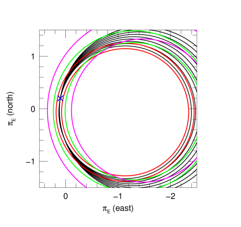
Figure 1: Evolution of parallax circles from individual photometric measurements. The black circles are the locus of ${\mbox{\boldmath$\pi$}}_{\rm E}$ consistent with individual measurements after (1,5,9,13,17,21,25,29,33) days of daily Spitzer observations, under the assumption of perfect ($\sigma=0$) photometric measurements, for a hypothetical $t_{\rm E}=30\,$day event that peaks at $u_{0,\oplus}=0$ on $t_{0}=\,$25 May 2019 and for which the first Spitzer observation is 9 July 2019, i.e., at $\Delta\tau=1.5$. The parallax is $(\pi_{{\rm E},N},\pi_{{\rm E},E})=(0.2,0.1)$ (blue cross). The pairs of red, green, and magenta circles show the $1\,\sigma$ error range for the measurements at days 1, 17, and 33, respectively, assuming photometric measurement errors $\sigma=0.01\,$mag. While the black circles all cross the true parallax value, the finite $1\,\sigma$ ranges (which grow with time) lead to a joint solution in the shape of an arc. See Figure 2.

I note that for simplicity of exposition, I have imagined satellite observations that take place well after Earth-based peak, i.e., $\Delta t=t_{\rm sat}-t_{0,\oplus}>0$. However, the formula applies equally well to single observations that are taken at any time. In particular, this includes single observations that take place well before Earth-based peak, i.e., $\Delta t<0$. There are many practical cases of this in real observations as well.

3 Impact of Realistic Conditions on Ideal Case

Equation (12) applies quite generally to the idealized case. However, because almost 800 microlensing events have been observed with Spitzer, it is important to understand how this idealization relates to this ensemble of real observations.

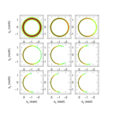
Figure 2: Evolution of an arc. Successive panels show the ${\mbox{\boldmath$\pi$}}_{\rm E}$ error contours after (1,5,9,13,17,21,25,29,33) days of daily Spitzer observations, with measurement errors $\sigma=0.01\,$mag, for the same hypothetical event illustrated in Figure 1, which has true parallax $(\pi_{{\rm E},N},\pi_{{\rm E},E})=(0.2,0.1)$. The colors (black, red, yellow, green) indicate $\Delta\chi^{2}<(1,4,9,16)$. The contours evolve slowly from a circle to an arc, but cease after the sixth panel $(\Delta\tau=2.4)$ because the errors on the radii ($u_{\rm sat}/Q)$ of the successive degenerate circles become too large for the additional observations to contribute. See Equation (15) and Figure 1.

One important practical point to keep in mind is that for Spitzer observations toward the bulge, the vector ${\bf Q}$ points roughly due west and its amplitude lies approximately in the range

$$Q\simeq 1+\sin[8^{\circ}\times(Y-2013)\pm 18^{\circ}],$$ (14)

where $Y$ is the year of observation. The direction simply reflects the facts that Spitzer is in an Earth-trailing orbit and that for Galactic-bulge targets, the ecliptic is roughly parallel to the equator. Then, because the 2014-2019 campaigns have taken place when the bulge is approximately in opposition (while $t_{0,\oplus}$ is almost always within $\sim 1.5\,$ months of opposition), the ${\bf v}_{\oplus}\Delta t$ term in Equation (10) approximately “corrects” the Earth position going into “${\bf D}$” to what it would be at the time of the Spitzer observation. On the other hand, due to Sun-angle restrictions, Spitzer observations toward the ecliptic are always near quadrature. This accounts for the form of Equation (14). The normalization and range reflect the fact that in 2013, the bulge was in opposition at the midpoint of the 38-day Spitzer viewing window.

Continuing to restrict attention to “high-magnification” ($u_{0,\oplus}\ll 1)$ events, there are two main differences between real observations and the idealized case of Section 2. First, there are in practice not just two observations, but a series of observations that either begin well after $t_{0,\oplus}$ or end well before $t_{0,\oplus}$. Second, the value of $u_{\rm sat}$ for each observation is not known precisely but with some finite error.

Regarding the errors, both quantities that enter the circle center in Equation (13) (${\bf Q}$ and $\Delta\tau$) are precisely known, so the only uncertainty in the description of the circle is in its radius. This derives from the error in the value of $u_{\rm sat}$, which propagates via Equation (5) from $A_{\rm sat}=1+(f_{\rm sat}-f_{\rm base,{\rm sat}})/f_{s,{\rm sat}}$. Thus, there are three potential sources of error: the individual measurement error $f_{\rm sat}$, the estimate of the baseline flux $f_{\rm base,{\rm sat}}$, which in practice comes from the overall fit to the satellite light curve, and the satellite source flux $f_{s,{\rm sat}}$, which comes from the color-color relation.

The last of these puts a fundamental limit on the precision in the sense that this error cannot be improved by additional observations. However, as I now show, its impact is usually small. The color-color relation yields an error in magnitudes, e.g., $\sigma=0.04\,$mag. Propagating through Equation (5), we obtain $\sigma(A_{\rm sat})=(A_{\rm sat}-1)k\sigma$, where $k=0.4\ln 10$, and so

$$\sigma_{0}(u_{\rm sat})={\sigma(A_{\rm sat})\over|dA/du|}=\biggl{(}{A-1\over A}\,{u(u^{2}+2)(u^{2}+4)\over 8}\biggr{)}k\sigma.$$ (15)

The coefficient in brackets is relatively small and stable over the relevant range of $u$, taking on values of $(0.29,0.22,0.27,0.37,0.50)$ for $u=(0.5,1.0,1.5,2.0,2.5)$. Therefore, we expect that the limit on the width of the circle in the ${\mbox{\boldmath$\pi$}}_{\rm E}$ plane due to the color-color relation will be small, For example, for $\sigma=0.04\,$mag and $Q=1.3$, this limit would be $\sigma_{0}\lesssim 0.01$ over the range $0.5<u_{\rm sat}<2$.

The error due to the individual flux measurement errors (expressed in magnitudes $\sigma_{i}$) degrades much more rapidly with increasing $u$. Ignoring the other two sources of error (color-color relation and baseline flux) and considering the case of zero blending, this can be evaluated

$$\sigma_{i}(u_{\rm sat})=\biggl{(}{u(u^{2}+2)(u^{2}+4)\over 8}\biggr{)}k\sigma_{i}.$$ (16)

For the same five values of $u=(0.5,1.0,1.5,2.0,2.5)$, the coefficient in brackets takes on values of $(0.60,1.9,5.0,12,39)$. Thus, for observations that begin outside the Einstein ring $(u_{\rm sat}>1)$, the parallax information content is dominated by the earlier observations. This has important implications, which I discuss immediately below. The last source of error (in $f_{s,\rm base}$) generally plays the role of exacerbating this effect: it is subdominant in the early observations, while the later-time observations mainly contribute to evaluating $f_{s,\rm base}$ itself.

Based on this assessment of the errors, I now show that the main impact of a finite series of observations (relative to a single observation) is usually to partially break the complete-circle degeneracy and turn it into an arc (e.g., Figure 5 of Jung et al. 2019). The first point to note is that for most late-starting observations, $Q\gg\pi_{\rm E}$. That is, typically $Q\sim 1$ while $\pi_{\rm E}\lesssim 0.2$ for most events. Moreover the direction of ${\bf Q}$ changes very little with time because ${\bf D}$ and ${\bf v}_{\oplus}$ are both approximately aligned with the ecliptic. Therefore, the center of the circle $(\Delta\tau/Q)({\bf Q}/Q)$ is gradually moving west while its eastern limb must always pass (within errors) through ${\mbox{\boldmath$\pi$}}_{\rm E}$, which is near the origin. Thus, the arcs comprising the eastern limbs of circles from multiple epochs will largely coincide, while the western limbs will increasingly separate, i.e., be inconsistent with one another. See Figure 1. However, as discussed in the previous paragraph, the width of these circles is rapidly increasing, so that most of their constraining power comes from the earlier measurements. For this reason, the process tends to leave parallax arcs, which (other things being equal) are longer for observations sequences that start at higher $u_{\rm sat}$. See Figure 2.

4 Resolution of 1-D Degeneracy

As discussed in Section 3, multiple late-time measurements will always restrict the circle described by Equations (12) and (13) to an arc. And if these observations begin early enough, then the arc (or arcs, see below) will be sufficiently restricted to regard them as 2-D (rather than 1-D) measurements. In fact, if the measurements begin sufficiently early, one should just recover the two-fold degeneracy predicted by Refsdal (1966) and illustrated by Figure 1 of Gould (1994). That is, with improving information, the arc should break up into two arclets placed symmetrically with respect to the ${\bf Q}$ (essentially, ${\bf D}$) axis.

However, in this section, I want to focus on how this 1-D arc (or even circle) degeneracy can be broken for the cases that the arc is relatively long. There are two classes of methods: information from annual parallax, and independent information about the direction of the lens-source relative proper motion ${\mbox{\boldmath$\mu$}}_{\rm geo}$. For the second class, there are three known distinct approaches.

4.1 Combining with 1-D Annual Parallax Measurements

A very large fraction of microlensing events, at least among those that are bright enough to allow Spitzer observations, have sufficient information for 1-D parallax measurements. These are usually straight in the Cartesian ${\mbox{\boldmath$\pi$}}_{\rm E}$ plane. See, for example, Figure 3 of Park et al. (2004), Figure 4 of Ghosh et al. (2004), Figure 2 of Jiang et al. (2004), and Figure 1 of Poindexter et al. (2005). The reason that these are all very old papers, from an era when the rate of microlensing-event discovery was $\sim 5$ times lower than today, is that the main scientific interest was in the effect itself and its potential applications, rather than in the $\pi_{\rm E}$ measurement, which was generally too weak to be useful. However, there have been some cases for which such 1-D measurements did play a significant role in the immediate scientific results, e.g., Figure 2 of Dong et al. (2009), Figure 3 of Batista et al. (2009), and Figure 6 of Muraki et al. (2011).

Such linear 1-D contours will in general intersect the circle described by Equations (12) and (13) in two places. Hence, in the general case, the two intersection points will yield different values of $\pi_{\rm E}$, with the fractional difference being greater when the 1-D contours are farther from being tangent to the circle. However, if the parallax circle has been broken into sufficiently small arclets, then this two-fold discrete degeneracy may be automatically broken by inconsistency at one of the two intersection points.

I note that confusion with xallarap effects due to orbital motion of the source is a potentially more serious problem in the interpretation of 1-D annual parallax compared to 2-D. (Xallarap has no direct effect on space-based parallaxes, but is relevant here because I am investigating 1-D annual parallax as a means to break the space-based parallax degeneracy.) Xallarap can, in principle, always perfectly mimic annual parallax. However, as pointed out by Poindexter et al. (2005) it is extremely unlikely that, for 2-D parallax, the three principal xallarap parameters (period, phase, and inclination) would all precisely mimic those induced by Earth’s motion. But in the case of a putative 1-D annual parallax signal, there is no such strong test against xallarap: any method of producing uniform acceleration for the main duration of the event will have exactly the same effect on the light curve. It is still the case that xallarap is a priori much less likely than parallax because the Sun is definitely accelerating Earth in its direction, while only a small fraction of source stars have companions in the mass and separation range where they could induce acceleration that is both uniform (i.e., with sufficiently large semi-major axis) and of sufficient strength (i.e., with sufficiently small semi-major axis and sufficiently large mass) to produce the observed effect. Nevertheless, this possibility should be evaluated concretely in each individual case.

4.2 Combining with Independent Proper-Motion Information

The direction of ${\mbox{\boldmath$\pi$}}_{\rm E}$ is by definition the same as the direction of ${\mbox{\boldmath$\mu$}}_{\rm geo}$, i.e., the lens-source relative proper motion in the geocentric frame. Therefore, if this direction is known, then even the full circular degeneracy from Equation (13) can be unambiguously resolved.

There are three known methods to independently measure the lens-source relative proper motion. One of these directly measures ${\mbox{\boldmath$\mu$}}_{\rm geo}$, a second directly measures the heliocentric proper motion ${\mbox{\boldmath$\mu$}}_{\rm hel}={\mbox{\boldmath$\mu$}}_{\rm geo}+{\bf v}_{\oplus}(\pi_{\rm rel}/{\rm AU})$, while a third directly measures something that is intermediate. The relationship between ${\mbox{\boldmath$\mu$}}_{\rm geo}$ and ${\mbox{\boldmath$\mu$}}_{\rm hel}$ has been analyzed in detail by Ghosh et al. (2004) and by Gould (2014), and there are no further issues to be explored here. I mention this issue only for completeness.

Note that because $\theta_{\rm E}=\mu_{\rm geo}t_{\rm E}$ and $t_{\rm E}$ is measured during the event, each of these methods also yields $\theta_{\rm E}$, which is the other parameter (in addition to $\pi_{\rm E}$) that is required to measure $M$ and $\pi_{\rm rel}$.

4.2.1 Proper Motion From Astrometric Microlensing

The light centroid of the two magnified images is displaced from the true position of the source by,

$$\delta{\mbox{\boldmath$\theta$}}=-{\Delta{\mbox{\boldmath$\theta$}}\over(\Delta\theta/\theta_{\rm E})^{2}+2},$$ (17)

where $\Delta{\mbox{\boldmath$\theta$}}$ is the displacement of the lens relative to the source (Miyamoto & Yoshii, 1995; Hog et al., 1995; Walker, 1995). Thus, by a series of astrometric measurements (and initially excluding those near the microlensing event) one can solve for the source parallax $\pi_{s}$ and proper motion ${\mbox{\boldmath$\mu$}}_{s}$. Then one can apply Equation (17) to the deviations $\Delta{\mbox{\boldmath$\theta$}}$ from this solution to determine $\theta_{\rm E}$ and the lens-source relative proper motion. In practice, one would fit all the astrometric data to all of these parameters simultaneously.

Note that if the event is relatively short, then the astrometric deviations occur while Earth’s motion is similar to that at $t_{0,\oplus}$, so it is the geocentric proper motion that is most directly measured. If the event is long, then the measurements are most sensitive to the heliocentric proper motion. In practice, there is no ambiguity. One just, for example, fits for the heliocentric proper motion and that quantity will be returned by the fitting program. The distinction is just that if the event is short, the error bars on a fit to ${\mbox{\boldmath$\mu$}}_{\rm geo}$ will be smaller than on ${\mbox{\boldmath$\mu$}}_{\rm hel}$.

4.2.2 Proper Motion By Resolving the Einstein Ring

With sufficiently high resolution, the two images of the source can be resolved. In this case, the separation between the two images and their flux ratio directly yields $\theta_{\rm E}$, while their orientation (position angle $\psi$) on the sky gives the direction of the instantaneous lens-source separation $\Delta{\mbox{\boldmath$\theta$}}$. The first such image resolution was recently achieved by Dong et al. (2019) using VLTI GRAVITY.

While the direction of lens-source separation $\Delta{\mbox{\boldmath$\theta$}}$ does not directly give the direction of lens-source relative proper motion ${\mbox{\boldmath$\mu$}}_{\rm geo}$, the angle between these two vectors is precisely known from the photometric light curve, or from the flux ratio of the two images. Unfortunately the sign of this angle (same as the sign of $u_{0,\oplus}$) is not known, and this degeneracy remains even for the case that we are still considering, $|u_{0,\oplus}|\ll 1$. In principle, this discrete degeneracy can be resolved by a second epoch of high-resolution imaging, e.g., 1 day later. However, Dong et al. (2019) were unable to obtain a second epoch due to weather. In such cases, this degeneracy may be resolved by either of the two methods mentioned above, i.e., by astrometric microlensing or by 1-D annual parallax. In those cases, either method would itself give a measurement of the proper-motion direction, but direct imaging of the Einstein ring gives vastly more precise results. Hence, the main role of these auxiliary techniques would simply be to break the degeneracy (Dong et al., 2019). Finally, this degeneracy could in principle be resolved by the Spitzer observations if these restricted the circle to an arc that intersects one but not both solutions.

4.2.3 Proper Motion From Late-Time Imaging

Finally, after the lens and source separate sufficiently to be separately resolved (Alcock et al., 2001) or at least to distort their common unresolved image (Bennett et al., 2006), then their relative proper motion can be determined simply by dividing their measured vector separations by the elapsed time since $t_{0,\oplus}$.

In contrast to the previous three methods, which do not depend in any way on the lens being luminous, this method appears at first sight to require a luminous lens. And it therefore appears to be less valuable, because if the lens can be imaged (which automatically yields $\mu$ and so an estimate of $\theta_{\rm E}=\mu_{\rm geo}t_{\rm E}$), then good estimates of $M$ and $\pi_{\rm rel}$ can already be made from its photometric properties combined with the constraint $\theta_{\rm E}^{2}=\kappa M\pi_{\rm rel}$. However, as discussed by Gould (2014), this “lower value” is somewhat deceptive. For several tens of percent of cases, the star that is imaged will actually be a binary companion to a dimmer (or possibly dark) lens. The proper motion of this companion will be nearly identical to that of the lens, but its photometric properties will be completely unrelated to those of the lens. Such cases can only be detected and analyzed if there is an independent measurement of the microlens parallax. Because the proper motion is measured by this imaging, all that is required to extract a full 2-D determination of ${\mbox{\boldmath$\pi$}}_{\rm E}$ is a 1-D parallax. This could come from 1-D annual parallax (Ghosh et al., 2004; Gould, 2014), or from a circle (or arc) as investigated in the current work.

5 General Case of a Single Late-Time Observation

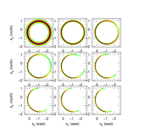
Figure 3: Similar to Figure 2 except that the event as seen from Earth has $u_{0,\oplus}=+0.4$ (rather than 0). Note that the symmetry axis is inclined to the ${\bf Q}$ axis (basically east-west) by $\simeq\tan^{-1}(u_{0}/\Delta\tau)$, i.e., the same as the angle between ${\bf P}_{\rm E}$ and ${\mbox{\boldmath$\pi$}}_{\rm E}$ (see Eq. (18)). This is contrary to the case that the satellite observations cover the peak (Refsdal, 1966; Gould, 1994). Because the offset between the two degenerate solutions is larger ($|{\mbox{\boldmath$\pi$}}_{{\rm E},++}-{\mbox{\boldmath$\pi$}}_{{\rm E},+-}|\sim 1.6$ versus $\sim 0.4$ for $u_{0,\oplus}=0$ from Fig. 2), the large arc tends to break up into two arclets, although only marginally for the adopted measurement errors $\sigma=0.01\,$mag shown here.

I began by investigating the special case of high-magnification ($u_{0,\oplus}$) because it captures the essential physics and is mathematically simple. But it is important to also explore the more general case. To facilitate this investigation, I introduce ${\mbox{\boldmath$\pi$}}_{\rm E}^{T}$, which I define as having the same magnitude as ${\mbox{\boldmath$\pi$}}_{\rm E}$ ($|{\mbox{\boldmath$\pi$}}_{\rm E}^{T}|=\pi_{\rm E}$), but whose direction is orthogonal (${\mbox{\boldmath$\pi$}}_{\rm E}^{T}\cdot{\mbox{\boldmath$\pi$}}_{\rm E}=0$). And I introduce another vector

$${\bf P}_{\rm E}\equiv{(\Delta\tau){\mbox{\boldmath$\pi$}}_{\rm E}+u_{0}{\mbox{\boldmath$\pi$}}_{\rm E}^{T}\over\sqrt{(\Delta\tau)^{2}+u_{0}^{2}}},$$ (18)

which also has the same magnitude ($|{\bf P}_{\rm E}|=\pi_{\rm E}$) but is rotated relative to ${\mbox{\boldmath$\pi$}}_{\rm E}$ by $\tan^{-1}(u_{0}/\Delta\tau)$. Note that I have suppressed the “$\oplus$” subscript on $u_{0}$. Then, Equation (9) becomes

$$u_{\rm sat}^{2}=\bigg{|}{{\mbox{\boldmath$\pi$}}_{\rm E}\Delta\tau\over\pi_{\rm E}}-{\bf Q}\pi_{\rm E}+{{\mbox{\boldmath$\pi$}}_{\rm E}^{T}\over\pi_{\rm E}}u_{0}\bigg{|}^{2}$$ (19)

or

$$u_{\rm sat}^{2}=(\Delta\tau)^{2}+u_{0}^{2}-2{\bf Q}\cdot{\bf P}_{\rm E}\sqrt{(\Delta\tau)^{2}+u_{0}^{2}}+Q^{2}P_{\rm E}^{2}.$$ (20)

Similarly to Equation (11), this can be rewritten as

$$u_{\rm sat}^{2}=\bigg{|}Q{\bf P}_{\rm E}-{{\bf Q}\over Q}\sqrt{(\Delta\tau)^{2}+u_{0}^{2}}\bigg{|}^{2}$$ (21)

or

$$\bigg{|}{\bf P}_{E}-{{\bf Q}\over Q^{2}}\sqrt{(\Delta\tau)^{2}+u_{0}^{2}}\bigg{|}^{2}=\biggl{(}{u_{\rm sat}\over Q}\biggr{)}^{2}.$$ (22)

That is, formally, ${\bf P}_{\rm E}$ traces a circle with center $\sqrt{(\Delta\tau)^{2}+u_{0}^{2}}{\bf Q}/Q^{2}$ and radius $u_{\rm sat}/Q$,

$${\bf P}_{\rm E}=\sqrt{(\Delta\tau)^{2}+u_{0}^{2}}{{\bf Q}\over Q^{2}}+{u_{\rm sat}\over Q}\hat{\bf n}.$$ (23)

I now express this vector equation in a specific coordinate system, in which the $x$-axis is aligned with ${\bf Q}$ and the $y$-axis is orthogonal to it. The center of the ${\bf P}_{\rm E}$ circle is then at $(\sqrt{(\Delta\tau)^{2}+u_{0}^{2}},0)$. Because ${\bf P}_{\rm E}$ and ${\mbox{\boldmath$\pi$}}_{\rm E}$ are related by a simple rotation of $\pm\tan^{-1}(u_{0}/\Delta\tau)$ (depending on the sign of $u_{0}$) the contour for ${\mbox{\boldmath$\pi$}}_{\rm E}$ will still be a circle of the same radius, but with its center rotated by this angle. That is, in this same coordinate system,

$${\mbox{\boldmath$\pi$}}_{{\rm E},\pm}(\phi)={(\Delta\tau,\pm|u_{0}|)+(\cos\phi,\sin\phi)u_{\rm sat}\over Q},$$ (24)

where $\phi$ parameterizes the position around the circle, and the “$\pm$” subscript shows the solutions for the two different signs of $u_{0}$ (i.e., $u_{0,\oplus}$). That is, there are two circles of the same size, whose centers are offset by $\pm u_{0}/Q$ in the direction orthogonal to ${\bf Q}$.

Figure 3 shows the results of the same observation sequence as Figure 2 but assuming that the otherwise identical event has $u_{0,\oplus}=+0.4$. Note that axis of symmetry is inclined to the ${\bf Q}$ axis (essentially the east-west axis) by about $\tan^{-1}(u_{\rm sat}/\Delta\tau)$. This is contrary to usual case, which was analyzed by Refsdal (1966) and Gould (1994), for which the symmetry axis is along the Earth-satellite separation vector. Also note that in this case, the single arc is beginning to break up into arclets, one centered on each of the two degenerate solutions.

6 Discussion

While I began my investigation of circular microlens-parallax degeneracies with the specific aim of understanding the ${\mbox{\boldmath$\pi$}}_{\rm E}$ “arcs” that appear in microlensing events with late-time Spitzer observations, these circular degeneracies are actually a powerful tool for understanding space-based microlensing parallaxes more generally. In fact, as mentioned in Section 2, Equations (12), (13), (23), and (24) actually apply to any individual space-based observation (provided that $F_{s,{\rm sat}}$ and $F_{s,\rm base}$ are known).

6.1 Parallax Circles: A General Tool

That is, any ensemble of satellite microlensing parallax observations can be understood as an overlapping set of circles on the ${\mbox{\boldmath$\pi$}}_{\rm E}$ plane. In Section 3, I gave one application of this approach to understand how these overlapping circles combine to form arcs for events with only late-time satellite observations.

Figure 4: Five single-measurement circular degeneracy contours in the ${\mbox{\boldmath$\pi$}}_{\rm E}$ plane shown for an event with $u_{0,\oplus}=+0.4$, $t_{\rm E}=18\,$days and $t_{0,\oplus}=$18 July 2019. The five simulated Spitzer measurements are (left to right) at $\Delta\tau=(t-t_{0,\oplus})/t_{\rm E}=(-0.5,0,+0.5,+1.0,+1.5)$. The spacing of the concentric circles shows $\pm 1\,\sigma$ errors propagated from measurement errors of $\pm 0.01\,$mag. Any combination of two of the first three observations would give a very precise measurement of ${\mbox{\boldmath$\pi$}}_{\rm E}$ (up to a two-fold degeneracy). However, because one does not know a priori how the space and ground events are offset, roughly four measurements would be necessary to reasonably guarantee good precision (plus an additional measurement at baseline). See Calchi Novati & Scarpetta (2016) for a view of the parallax geometry in the heliocentric-observer (as opposed to ${\mbox{\boldmath$\pi$}}_{\rm E}$) plane.

6.2 Understanding the Four-Fold Degeneracy

A second application is to provide an alternate understanding of the four-fold degeneracy. Let us first consider the case of $u_{0,\oplus}=0$, for which there is a two-fold degeneracy. The circles are always centered on the ${\bf Q}$ axis. They all must pass through the actual value of ${\mbox{\boldmath$\pi$}}_{\rm E}$. In doing so, they must also pass through ${\mbox{\boldmath$\pi$}}_{\rm E}^{\prime}=2[({\bf Q}/Q)\cdot{\mbox{\boldmath$\pi$}}_{\rm E}]({\bf Q}/Q)-{\mbox{\boldmath$\pi$}}_{\rm E}$, which is as much “below” the ${\bf Q}$ axis as ${\mbox{\boldmath$\pi$}}_{\rm E}$ is above it. Because this expression depends only on the direction of ${\bf Q}$ and not its magnitude, all circles that pass through ${\mbox{\boldmath$\pi$}}_{\rm E}$ will also pass through ${\mbox{\boldmath$\pi$}}_{\rm E}^{\prime}$ provided that this direction does not change. Hence, breaking this degeneracy (from satellite data alone) depends on ${\bf Q}$ changing direction enough to have a significant effect.

For the case of $u_{0}\not=0$, the picture of intersecting circles while the source is within the Einstein ring directly reproduces the traditional understanding of the two-fold degeneracy between the source passing on the same versus opposite sides of the lens as seen from the two observatories. See Figure 4. However, as shown by Figure 3, the symmetry axis rotates at late times, thus providing some possibility that the late-time “arc” will be inconsistent with one of the two solutions.

6.3 Cheap Satellite Parallaxes at All Magnifications

The geometry shown in Figure 4 immediately gives rise to a third and fourth application. The third application is a generalization of the Gould & Yee (2012) proposal for “cheap space-based microlens parallaxes”. Recall that their proposal rested on obtaining a space-based image very near $t_{0,\oplus}$ and was restricted to high-magnification events $u_{0,\oplus}\ll 0$. However, using the circle picture, it is easy to see that two satellite observations (plus baseline) are all that are needed in principle to measure ${\mbox{\boldmath$\pi$}}_{\rm E}$. That is, two circles, regardless of relative size, can only intersect in zero, one, or two places. Parallax circles must intersect at least once (within errors) at ${\mbox{\boldmath$\pi$}}_{\rm E}$.

If the circles intersect in two places (i.e., cross rather than being tangent), then the $\Delta\chi^{2}=2$ error contour (containing $(1-e^{-1})=63\%$ of the probability) is given directly by the ellipse that passes through the four intersection points of the two sets of $1\,\sigma$ error-circles. Consider, for example, the two smallest-error circles in Figure 4. One sees from the inset that these intersection points are separated by $\Delta\pi_{{\rm E},N}=0.014$ along the ordinate and by $\Delta\pi_{{\rm E},E}=0.044$ along the abscissa. Hence $\sigma(\pi_{{\rm E},N},\pi_{{\rm E},E})=(\Delta\pi_{{\rm E},N},\Delta\pi_{{\rm E},E})/\sqrt{8}=(0.005,0.016)$.

While it is always possible “in principle” to determine $N$ parameters (in the case $N=2$) from $N$ measurements, there are two main practical issues that usually lead one to seek some redundancy, i.e., more data points. First, some measurements may turn out to be mathematically degenerate (or nearly degenerate). Second, usually one would like to have internal checks on the externally calibrated error bars. I address these issues in turn.

If the two circles are tangent (or nearly so), and therefore have effectively only one point of intersection, then (after taking account of measurement errors), their overlap will be an arc. I have already shown in Section 3 that such arcs are the natural consequence of a late-time series of satellite observations. The main way to avoid osculating circles (and so arc or even circle degeneracies) is to make the observations while the source is inside the Einstein ring as seen from the satellite. This is easier said than done because one does not know a priori when this will occur. Indeed, for very large $\pi_{\rm E}\gtrsim 1$, there is no guarantee that the source will even pass within the Einstein ring as seen from the satellite. Thus there is some chance that one or both of two well-chosen observations, e.g., at $t_{0,\oplus}\pm 0.5\,t_{\rm E}$ would fall outside the Einstein ring. Hence, a more aggressive approach would be to make the first two observation early, e.g., at $t_{0,\oplus}-0.5\,t_{\rm E}$ and $t_{0,\oplus}-0.3\,t_{\rm E}$, to determine whether the event was rising or falling and make a rough ${\mbox{\boldmath$\pi$}}_{\rm E}$ measurement. And then to use these to decide on one or two additional measurements (in addition to baseline). Still, only of order $4+1=5$ observations would be needed. While more than the absolute minimum of $2+1=3$, it is still far less than in the current mode. See Figure 4.

Note that this approach could not be applied to Spitzer microlensing for three reasons. First, the observations are initiated with a 3-10 day delay. See Figure 1 of Udalski et al. (2015). This means that the great majority of events have their first observation after $t_{0,\oplus}-0.5\,t_{\rm E}$, which very often proves to be near or after $t_{0,{\rm sat}}+0.5\,t_{\rm E}$. Second, there is no way to alter the observing schedule on a daily basis as envisaged in the previous paragraph. Third, the data are not downloaded fast enough to make such real time decisions. However, if a satellite were specifically engineered for microlens parallaxes, then it could incorporate these capabilities. This would make it possible to monitor 1500 microlensing events per year with only 30 observations per day, which implies that a very small telescope (e.g., 20 cm) would be adequate.

A second reason for obtaining $4+1$ (rather than $2+1$) observations is to control systematics, i.e., deviations of the measured versus true values that are not captured by the statistical error bars. These can take a variety of forms, but the two of greatest concern are large random fluctuation (due to stochastic processes on either the sky, e.g., cosmic ray events, or the detector) and long-term trends. Of course, any satellite undergoes extensive commissioning observations at the start of the mission that are matched to its envisaged scientific goals, which would characterize such systematics in the present case. Still, it would be useful to have ongoing checks against large stochastic outliers, which would be a routine by-product of $(4+1)$ observations. (It is likely that the $\sim 1\,$hr exposures mentioned above would be subdivided into several sub-exposures, which would provide additional redundancy.)

The problem of long term trends (so-called “red-noise”) is substantially less severe when parameters are derived from a few measurements (the present case) as opposed to many measurements (e.g., transiting planets). To understand this concretely, consider the Spitzer light curve of OGLE-2016-BLG-1045, in Figure 1 of Shin et al. (2018). This shows long term residual trends with semi-amplitude $\sim 0.015\,$mag, which is approximately equal to the statistical errors. Suppose that one searched for a planetary transit in a region of a light curve containing $N=400$ points with these statistical and systematic error properties, and derived a transit with the same depth, i.e., 0.015 mag. If one treated the errors as being purely statistical at $\sigma=0.015\,$mag, then the error in the transit depth would be $\sigma/\sqrt{400}=0.00075\,$mag, so a clear $\Delta\chi^{2}=400$ planet “detection”. Even if one added the systematic “noise” $0.015/\sqrt{2}$ in quadrature to the statistical noise, one would still end up with a spurious $\Delta\chi^{2}=267$ “detection” (if one continued to treat the 400 individual measurements as independent).

But note that no such issue of “red” (i.e., correlated) noise arises in the single-epoch measurement tested by Shin et al. (2018) for OGLE-2016-BLG-1045. The one measurement that they use has an empirically renormalized error bar that automatically takes account of deviations due to both long term trends and statistical fluctuations. It does not take account of correlations, but since there is only a single measurement, correlations do not play any role.

The situation is only slightly worse for the two-measurement determinations envisaged here. That is, if the error bars were set to account for both random fluctuations and systematic trends (as in case of OGLE-2016-BLG-1045), then the pairs of error circles in Figure 4 would each individually be correct. It would not be correct to treat two measurements as statistically independent, but if one did so nevertheless (and if, e.g., the amplitude of systematic trends were equal to the statistical fluctuations as in OGLE-2016-BLG-1045), then one would only underestimate the true error of the ${\mbox{\boldmath$\pi$}}_{\rm E}$ determination by factor $\sqrt{6/5}\sim 1.1$. Of course, one should not proceed in this naive way, but rather take proper account of the actual error properties of the data. Nevertheless this exercise shows that “red noise” is a relatively minor issue for parameter measurements based on a few measurements unless the red noise itself is very severe. For the case of Spitzer, Zhu et al. (2017a) found severe red noise in only a small fraction of the order 50 events with data adequate to make this determination. The origin of these systematics is not precisely known, but is unlikely to affect an optical satellite with subsampled pixels of near uniform response, which (in contrast to Spitzer) would permit standard difference imaging analysis (DIA, Alard & Lupton 1998).

Figure 5: Illustration of degeneracy breaking using two satellites. The two pairs of thin-lined concentric circles are exactly the same as the parallax circles in Figure 4 that are closest to peak, namely at $\Delta\tau=(t-t_{0,\oplus})/t_{\rm E}=-0.5$ and $+0.5$ and for exactly the same simulated event. The intersect at the true parallax $(\pi_{{\rm E},N},\pi_{{\rm E},E})=(0.2,0.1)$, but also at a second degenerate solution, $(\pi_{{\rm E},N},\pi_{{\rm E},E})\simeq(-0.7,0.1)$. Indeed parallax circles at all epochs intersect at approximately the same locations. See Figure 4. The thick-lined concentric circles correspond to measurements made by a hypothetical second satellite in a Spitzer like orbit but launched exactly six years later and so not as far from Earth. These circles also intersect in two degenerate location, i.e., $(\pi_{{\rm E},N},\pi_{{\rm E},E})=(0.2,0.1)$ and $(-0.9,0.1)$. Combining the measurements of the two satellites resolves the degeneracy in favor of the first solution.

6.4 Cheap Breaking of the Four-Fold Degeneracy

The simplified approach outlined above would still leave the four-fold degeneracy in tact. In many cases this could be broken by one of the four methods outlined in Section 4. However, this simplified approach also makes it feasible to carry out the monitoring with two such satellites, as originally envisaged by Refsdal (1966). If both satellites were near the ecliptic (by far the cheapest approach), then only one pair of degeneracies would generally be broken. This was the outcome when Zhu et al. (2017b) applied this two-satellite technique, using Spitzer and Kepler, both of which are near the ecliptic. However, the degeneracy that was broken (between $\Delta\beta^{\prime}_{\pm,\mp}$ and $\Delta\beta^{\prime}_{\pm,\pm}$, i.e, opposite versus same signs) is by far the more important one because it would lead to different magnitudes of $\pi_{\rm E}$ and so different lens masses $M=\theta_{\rm E}/\kappa\pi_{\rm E}$ and lens-source relative parallaxes $\pi_{\rm rel}=\theta_{\rm E}\pi_{\rm E}$. Thus, a second, small, low-cost satellite would be by far the simplest and most robust method to systematically remove this degeneracy. See Figure 5